Improving snow simulations through improved representations of vegetation conditions: insights from high resolution simulations over California

Most hydrological models underestimate snow water equivalent (SWE) in the mountainous western US. Key limitations may include inadequate representation of spatial variability due to coarse-resolution precipitation input and inadequate representations of snow-vegetation interactions. Vegetation affects snow dynamics through snow interception, throughfall/unloading, and energy transfer through the canopy, yet basin-scale studies on the vegetation effects are limited. To address this issue, we applied Noah-MP version 5.0 with a dynamic vegetation module over the Sacramento and San Joaquin River Basins in California at 1 km resolution. The model was driven by the Analysis of Record for Calibration (AORC) forcing at its native 1 km resolution and by the NLDAS-2 forcing downscaled from ∼ 12 to 1 km using the WRF-Hydro Meteorological Forcing Engine. We carried out eight model experiments driven by the two forcing datasets and two vegetation schemes over the two Basins. Compared to the 4 km PRISM and 1 km AORC, the downscaled 1 km NLDAS-2 forcing data shows higher precipitation and lower temperatures over the mountains, resulting in more snowfall and SWE, which is more consistent with in-situ SWE observations. Using the 1 km NLDAS-2 forcing, the default vegetation scheme that prescribes leaf area index (LAI) and vegetation cover fraction, produces excessive SWE on the ground, mainly because the strong canopy shading (too high LAI) reduces snowmelt, even though more snowfall is intercepted by the canopy. The dynamic vegetation module produces smaller LAI than the prescribed (more consistent with MODIS LAI) and thus leads to more shortwave radiation reaching the snow surface, thereby enhancing episodic melting during the accumulation season. Validation against in-situ snow data suggests that the use of dynamic vegetation model and the downscaled NLDAS-2 data perform the best. These findings highlight the importance of vegetation effects and downscaling of atmospheric forcing to improve the accuracy of snow modeling over the Southwest US.

1 Introduction

Snow Water Equivalent (SWE) is important in regions like California where snowpack plays a vital role in freshwater supply and management. Studies show that mountain snowpack contributes to 70 %–80 % of the total annual runoff yield in the western United States (Daly et al., 2000b; Li et al., 2017). With complex terrain and a Mediterranean climate, California experiences significant variability in precipitation amount and patterns, which affect snowpack in the Sierra Nevada mountains. Snow dynamics are impacted by multiple factors such as precipitation, temperature, topography, wind, and vegetation (Anderson et al., 2014; Mott et al., 2018). Despite significant advancements, most hydrological models produce less SWE in the Southwest US than is observed (Cho et al., 2022; Garousi-Nejad and Tarboton, 2022; Fang et al., 2022). Various global reanalyses like ERA, ERA-Land, MERRA-2 and GLDAS significantly underestimate SWE in the Southwest US due to their coarse resolution, deficiencies in model physics (e.g. melting processes) and lack of SWE data assimilation (Broxton et al., 2016). Furthermore, most land surface models (LSMs) produce less SWE even with advanced snow physics and complex radiation transfer schemes due to inaccurate atmospheric forcing data (Cho et al., 2022; Toure et al., 2016; Garousi-Nejad and Tarboton, 2022). For instance, the NCAR CLM v5.0 show that the western US watersheds are forcing (snowfall) dominant, and underrepresentation of forcing datasets brings high prediction uncertainty in these regions (Eldardiry et al., 2025). Noah-MP (Niu et al., 2011) used in the National Water Model (NWM) (at 1 km resolution) produces a better match with the Natural Resources Conservation Service Snowpack Telemetry Network (SNOTEL) data but still underestimates SWE by 20 %–30 % (Cho et al., 2022; Garousi-Nejad and Tarboton, 2022).

The interactions between snow and vegetation represents a critical component of SWE dynamics impacting hydrology, biodiversity, and ecosystem services. With diverse landscapes ranging from the coastal forests to the alpine meadows, California exhibits a complex interplay between snowpack accumulation and vegetation distribution (Rundel and Millar, 2016). Understanding the interactions are essential for predicting and managing water resources, drought, and flood, serving biodiversity, and mitigating the impacts of climate change on ecosystems. Snow cover and vegetation work in a feedback manner and play a significant role in ecosystem productivity across varying landscapes (Cook et al., 2008; Euskirchen et al., 2016). In the mountainous regions such as the Sierra Nevada, snow accumulation during the winter months serves as a primary water source for vegetation growth in the dry summer and helps sustain vegetation through prolonged droughts. The timing and duration of snowmelt influence the onset of plant growth, with earlier snowmelt generally leading to earlier vegetation green-up and extended growing seasons (Cooper et al., 2011; Livensperger et al., 2016). Vegetation, in turn, influences snow accumulation and melting processes through various biophysical feedback mechanisms. Forests, for example, can modify snowpack characteristics by reducing wind speed, intercepting snowfall, altering snowpack density, and reducing surface albedo through canopy shading (Niu and Yang, 2004; Bartlett and Verseghy, 2015; Stähli et al., 2009; Webster and Jonas, 2018). Shrubs and grasses in montane and subalpine ecosystems can also affect snow distribution by trapping snow in the winter and shading the snow surface in the spring, thus influencing the timing and magnitude of snowmelt runoff (Pomeroy et al., 2006; Sturm et al., 2005).

Studies examining the interactions between snow and vegetation range from advanced field observations to remote sensing and distributed modeling approaches. Field studies include (but are not limited to) measuring snow depth, density, sap flow, leaf area index (LAI), normalized difference vegetation index (NDVI), nutrient storage and transport, vegetation characteristics at various sites across different elevational gradients (Hwang et al., 2009; O'Keefe et al., 2020; Rey et al., 2021). Remote sensing techniques provide valuable tools for assessing snow-vegetation interactions over larger spatial scales. Satellite-based sensors, such as those aboard NASA's Landsat, MODIS and Copernicus's Sentinel missions, and airborne LiDAR offer insights into snow cover extent, vegetation phenology, and land surface properties. Tennant et al. (2017) used remotely sensed snow-cover information together with vegetation cover to quantify how vegetation influences seasonal snowpack patterns across western North America, while Wang et al. (2018) combined snow and vegetation observations to investigate how winter snow conditions affect subsequent vegetation activity in northern ecosystems. Thus, spatially and temporally collocated observations of snow cover/SWE and vegetation properties such as greenness, LAI, or vegetation cover can be used to evaluate the relationships and feedbacks between snow and vegetation. Numerical modeling approaches, including coupled snow-vegetation models, facilitate the integration of biophysical processes governing snow dynamics and vegetation responses (e.g., Niu and Yang, 2004). These models simulate snow accumulation, melt, and redistribution in conjunction with vegetation growth, productivity, and water use. By incorporating ecological parameters such as plant phenology, leaf area index, and root water uptake, these models provide insights into the complex feedback between snow and vegetation in regional ecosystems (Bonan et al., 2003; Franklin et al., 2020).

Modeling approaches to understand the interactions between snow and vegetation plays a crucial role in elucidating the complex dynamics of these two key components of the ecosystems. Numerical models serve as powerful tools for predictive understanding of the coupled processes governing snow accumulation, melt, and redistribution, as well as vegetation growth, productivity, and water use. By integrating physical, biological, and ecological processes, these models enable researchers to explore the feedback and interactions between snow and vegetation across different spatial and temporal scales. One prominent modeling approach used in studying snow-vegetation interactions is the use of LSMs. LSMs simulate the exchange of energy, water, carbon, and momentum between the land surface and the atmosphere, incorporating processes such as snow accumulation, melt, and sublimation, as well as vegetation dynamics (Overgaard et al., 2006). Noah-MP is one of the state-of-the-art LSM that simulates the complex snow-vegetation interactions through the dynamic leaf model and snow evolution scheme (Niu and Yang, 2004). The snow model of Noah-MP represents one of the best snow models compared to other LSMs like JULES, Catchment LSM, and Noah in modelling annual maximum SWE (Cho et al., 2022). However, compared to that of SNOTEL, Noah-MP tends to underestimate SWE depending on elevation ranges, and the higher elevation the larger underestimation of SWE partially due to underestimates of snowfall (Cho et al., 2022).

This study aims to (1) improve the accuracy of SWE simulation over California at 1 km resolution by enhancing precipitation estimates using a statistical downscaling approach, (2) advance understanding of how vegetation processes, including canopy snow interception, sublimation, and radiative effects (shading and scattering), influence snowpack accumulation and ablation, and (3) identify the optimal combination of precipitation forcing and vegetation representation for improving SWE estimation across California. To address these objectives, we employ Noah-MP version 5 with its dynamic vegetation model (Dickinson et al., 1998) that prognostically simulates leaf area index (LAI) and green vegetation fraction, enabling a detailed assessment of vegetation impacts on high-resolution snowpack simulations.

2 Study Area

The Noah-MP model was set up over two Hydrologic Unit Code, 4-digit (HUC-4) basins in California: the Sacramento and San Joaquin Rivers (Fig. 1). The Sacramento River Basin covers ∼ 70 000 km² in northern California and includes vast snow cover and forests in the southern Cascade Mountains, Klamath Mountains and Sierra Nevada (Domagalski, 1998). The San Joaquin River Basin covers an approximate area of 40 000 km² in central California. The 483 km long river originates in the Sierra Nevada mountains and meets the Sacramento River along its north-east border. Snowmelt runoff from the mountains is the main source of freshwater in the San Joaquin and Sacramento River Basins (Brekke et al., 2004). These two basins differ in their altitude and vegetation cover which can potentially impact the snow-vegetation interaction.

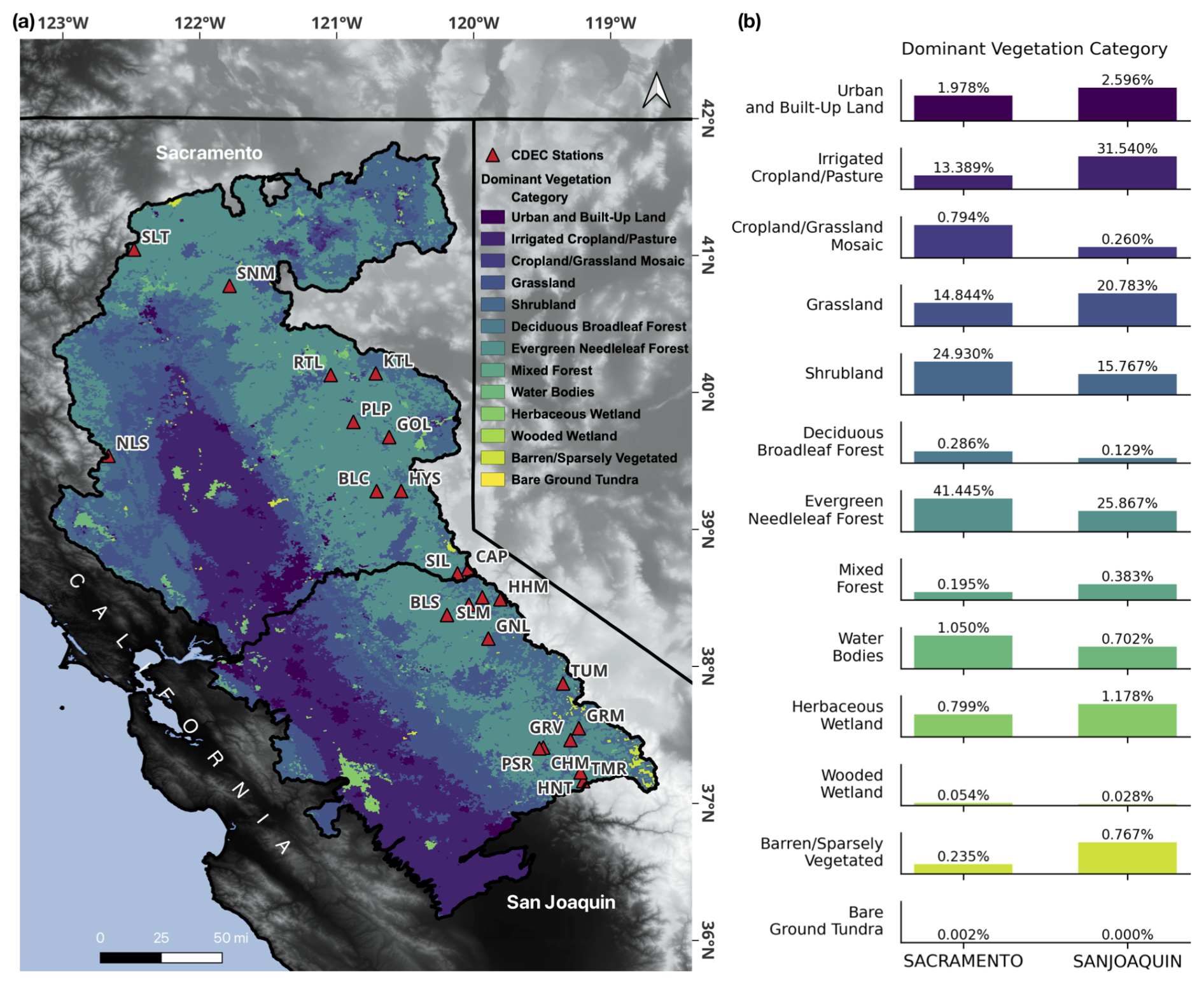
Figure 1 (a) Study Area representing the Sacramento and San Joaquin Basins (HUC4) in California with dominant vegetation types. The red triangles represent the Snow Water Equivalent (SWE) stations of the California Data Exchange Center (CDEC). (b) Percentage cover of dominant vegetation types in the two watersheds (Sacramento and San Joaquin).

3 Data

3.1 Forcing Data

We used two gridded meteorological forcing datasets including the Analysis of Record for Calibration (AORC) and the North American Land Data Assimilation System (NLDAS-2). These forcing datasets differ in their mean precipitation, with NLDAS-2 exhibiting systematically higher precipitation amounts than AORC. AORC version 1.1 was developed at National Weather Service as a part of development of the contiguous United States (CONUS) scale hydrologic modeling capability and establishment of the National Water Model (Kitzmiller et al., 2018). AORC is a meteorological forcing dataset at 1 km spatial resolution and hourly temporal resolution over CONUS region and provides 8 variables required to drive hydrological or land surface models. AORC data has been developed using the multiple sources, which includes NLDAS-2, LIV16, NEXRAD Stage IV, URMA, and a climatology from PRISM (Fall et al., 2023, JAWRA) over the NWM grid. AORC v1.1 is available from 1979–2023 as part of version 3 of the National Water Model (NWM). NLDAS-2 is a primary forcing for Phase 2 of the North American Land Data Assimilation System (NLDAS). The datasets are available at 1/8th-degree and hourly temporal resolution. It combines multiple observational data from gauge, satellite, and radar to produce the time­ series of meteorological variables (Xia et al., 2012). It extends from January 1979 to present over North America. We further downscaled this dataset to 1 km spatial resolution to match the AORC grids (see Sect. 4.2).

3.2 Validation data

To evaluate the performance of the meteorological forcing, snow processes, and vegetation dynamics in this study, multiple independent in-situ observations and gridded datasets were used. These datasets are grouped below according to the variables used for validation, including precipitation and temperature, snow, and leaf area index (LAI).

3.2.1 Precipitation and temperature validation

PRISM

We used PRISM (Parameter-elevation Regressions on Independent Slopes Model) daily data to evaluate precipitation and temperature from AORC and the downscaled NLDAS-2 data. PRISM, which is developed and maintained by the PRISM Climate Group at Oregon State University, provides high-resolution (4 km) daily climate data for various meteorological variables (Daly et al., 2000a). Monthly normals are the baseline datasets which are modeled using digital elevation model as a predictor grid and the daily normals are derived using the “nudging and smoothing” technique. The daily normals include precipitation, minimum, maximum and mean temperature, and minimum and maximum vapor pressure deficit over the CONUS. In this study we have used the daily temporal resolution temperature and precipitation datasets from PRISM. Note that all the 1 km datasets (AORC and downscaled NLDAS data) are averaged to 4 km resolution using bilinear interpolation for the comparison.

CDWR stations

California Cooperative Snow Surveys (CCSS), which is part of the California Department of Water Resources (CDWR), conducts snow surveys in the mountains of California (https://water.ca.gov/Programs/Flood-Management/Flood-Data/Snow-Surveys, last access: 11 September 2026). Established in 1929 by the California Legislature, this program is a partnership of more than 50 state, federal, and private agencies. CCSS maintains a total of 265 snow courses and 130 snow sensors located throughout the Sierra Nevada and Shasta-Trinity mountains. This study uses data from 23 CDWR stations across the study area to obtain precipitation, temperature, and SWE data (Fig. 1).

GHCN stations

The Global Historical Climatology Network (GHCN)-Daily dataset integrates observations from a wide range of sources that have been combined and subjected to rigorous quality control procedures (Menne et al., 2012). It includes several key meteorological variables such as daily maximum and minimum air temperature, temperature at the observation time, precipitation, snowfall, and snow depth. This dataset functions as the official repository for daily measurements within the Global Climate Observing System (GCOS) Surface Network (GSN) and is widely used for analyzing climate variability and extremes, including their frequency and intensity. We have chosen 177 precipitation and 178 temperature stations from the GHCN network. The stations with high quality data (> 95 % available data) were chosen for the analysis. The minimal missing data were filled using the long-term average.

3.2.2 Snow validation

NWM v3.0 SWE

To analyze the improvement in snow estimation with respect to current operational NWM we have downloaded 5-year (2015–2019) retrospective SWE estimation from NWM v3.0. NWM uses prescribed monthly LAI from look-up table, the Jordan (1991) scheme for rain-snow partitioning, the Ball-Berry scheme for stomatal resistance and the BATS scheme (Dickinson et al., 1993) for snow surface albedo. The retrospective simulations from NWM v3.0 are available for a period between 1979–2023 and can be downloaded from the Amazon Web Service (AWS) storage (https://registry.opendata.aws/nwm-archive/, last access: 11 September 2026). These datasets are available at 3-hourly, which we aggregated to daily timescale for daily comparison.

UA-SWE

UA snowpack data (UA-SWE), developed at the University of Arizona, is based on observed SWE and snow depth from Snow Telemetry (SNOTEL) and National Weather Service Cooperative Observer stations across CONUS (Broxton et al., 2024). Initially, UA-SWE was developed at 4 km daily resolution using the 4 km PRISM data, though they have recently been downscaled to 800 m resolution by using 800 m PRISM climate data, and accounting for the effects of smaller-scale topographic and forest cover variations (Broxton et al., 2024). Generally, the 800 m and 4 km versions are similar, except the 800 m version shows more detail and has a little less SWE in forested areas. This study uses the 800 m version of the UA-SWE dataset.

SNODAS

Snow Data Assimilation System (SNODAS) is a data assimilation system developed by National Operational Hydrologic Remote Sensing Center (NOHRSC) at NOAA (National Operational Hydrologic Remote Sensing, 2004). SNODAS provides snow cover estimates at 1 km and daily resolution to support the hydrological modeling and analysis. SNODAS assimilates data from satellite, airborne platforms, and ground stations. The main inputs to the SNODAS includes the downscaled outputs from numerical weather prediction (NWP) models to simulate the snow cover using a physically based, mass and energy balance snow model.

3.2.3 Vegetation (LAI) validation

MODIS and Sun Yat-Sen University LAI

This study uses the MOD15A2H Version 6.1 data from the Moderate Resolution Imaging Spectroradiometer (MODIS) sensor on-board the Terra satellite. MODIS captures data in 36 spectral bands (Myneni et al., 2021) and provides detailed information about the Earth's surface and atmosphere, including vegetation, land cover, and cloud properties. The MOD15A2H dataset is a combined LAI and Fraction of Photosynthetically Active Radiation (FPAR) product that is an 8 d composite with 500 m spatial resolution. In this study, we aggregate the 8 d product into seasonal data for comparison with the modelled data. We also used the reprocessed MODIS Version 6.1 LAI data from Land-Atmospheric Interaction Research Group at Sun Yat-Sen University (Lin et al., 2023). Their product applies spatio-temporal filtering and smoothing to the MODIS LAI data to reduce their spatial and temporal inconsistency. These datasets are also available at the 8 d temporal resolution and 500 m spatial resolution, which have been converted to seasonal data for comparison in this study.

4 Methods

4.1 Noah-MP version 5

Noah-MP was developed as a community effort to improve the Noah LSM by adding a vegetation canopy layer and incorporating multiple physics options to parametrize different land-surface processes (Niu et al., 2011; Yang et al., 2011; He et al., 2023). Recently Noah-MP has been upgraded to a modularized version, Noah-MP Version 5.0, which represents each process with one separate module (He et al., 2023). Noah-MP is a grid based columnar model, which calculates the precipitation partitioning into surface and subsurface fluxes through physical equations, while preserving the energy and mass balance at each time step. Biogeophysical and biogeochemical processes are separately calculated for different land use classes, which are based on United States Geological Survey (USGS) or MODIS land type data. Major processes include canopy interception, canopy evaporation/sublimation, snow accumulation, snowpack evaporation/sublimation, snowmelt, soil surface evaporation, transpiration, infiltration, surface runoff, and subsurface runoff. The infiltrated water moves further through the soil column following the Richard's equation in the vadose zone. Finally, the water leaving the bottom of the soil column is considered as groundwater recharge in Noah-MP.

The snow component in Noah-MP is a process-based, multi-layer, and multi-physics energy balance model. Its layered design enables the simulation of internal snowpack dynamics such as compaction, water storage, and refreezing. A thin surface layer is included to better capture turbulent energy exchanges, which, together with net radiation, represent the primary energy to the snow layer that control snowpack temperature and the energy available for melt (Niu et al., 2011). The model also considers the energy required to change a snow layer to the melting/freezing points as well as the latent heat involved in phase changes between liquid water and ice. The model also accounts for temporally variable snow surface albedo (Wang et al., 2020), vegetation shading/scattering of radiation (Niu and Yang, 2004), and fractional snow cover (Niu and Yang, 2007).

4.1.1 The Snow Interception Model in Noah-MP

The snow interception model of Noah-MP represents the mass balance of the ice and liquid water on the canopy. It represents loading and unloading of snowfall, interception of rainfall and dripping of the intercepted water, sublimation/evaporation of the ice/liquid water on the canopy, melt of the intercepted snow and freezing of the melt water and intercepted rain (Niu and Yang, 2004). Following Hedstrom and Pomeroy (1998), Noah-MP represents the snow interception rate (or loading rate) as

$$\begin{array}{}\text{(1)}& Q_{\mathrm{ice},\mathrm{intcp}}=(W_{\mathrm{ice},\max }-W_{\mathrm{ice}})\left(\mathrm{1}-e^{-P_{\mathrm{snow}}\mathrm{\Delta }t/W_{\mathrm{ice},\max }}\right),\end{array}$$

where Δt is the time step, and P_snow (kg m² s⁻¹), W_ice, and W_ice,max (kg m⁻²) are the snowfall rate, the canopy-intercepted snow, and the maximum canopy load for snow, respectively. W_ice,max adopts the scheme of Schmidt and Gluns (1991):

$$\begin{array}{}\text{(2)}& W_{\mathrm{ice},\max }=\mathrm{6.6}\times \left(\mathrm{2.7}+{\displaystyle \frac{\mathrm{46}}{{\mathit{\rho }}_{\mathrm{snowfall}}}}\right)\times \left(E_{\mathrm{LAI}}+E_{\mathrm{SAI}}\right),\end{array}$$

where ρ_snowfall is the bulk snowfall density [kg m⁻³], which is represented as a function of surface air temperature, E_LAI and E_SAI are the effective leaf area index [m² m⁻²] and the effective stem area index [m² m⁻²], respectively, both of which are not buried by snow. Assuming ρ_snowfall=100 kg m⁻³, W_ice,max is ∼ 50 times the maximum load for liquid water.

The snowfall rate below the canopy, Q_snow [mm s⁻¹], is

$$\begin{array}{}\text{(3)}& Q_{\mathrm{snow}}=\left(\mathrm{1}-F_{\mathrm{veg}}\right)\times P_{\mathrm{snow}}+Q_{\mathrm{ice},\mathrm{drop}},\end{array}$$

where the first term on the right hand-side represents canopy throughfall, and F_veg is the vegetation cover fraction. The rate of snow drops from the vegetated fraction, Q_ice,drop [mm s⁻¹] is updated as

$$\begin{array}{}\text{(4)}& Q_{\mathrm{ice},\mathrm{drop}}=\left(F_{\mathrm{veg}}\times P_{\mathrm{snow}}-Q_{\mathrm{ice},\mathrm{intcp}}\right)+Q_{\mathrm{ice},\mathrm{unload}},\end{array}$$

where the first term in the right hand-side represents the snowfall that is unable to be intercepted by the canopy, and Q_ice,unload is the canopy snow unloading rate depending on the canopy temperature and wind speed (Roesch et al., 2001; Niu and Yang, 2004). Note that the snowpack on the ground also receives liquid water dripping from the canopy and throughfall of rain to represent rain-on-snow events.

4.1.2 The Radiation Transfer Model in Noah-MP

Noah-MP represents vegetation shading and scattering effects on shortwave radiation using a modified two-stream radiation-transfer approximation (Niu and Yang, 2004; Yang and Friedl, 2003). Radiative transfer through the canopy is governed by the total canopy gap probability (P_c), defined as the sum of the between-crown gap probability (P_bc), determined by canopy geometry and solar zenith angle, and the within-crown gap probability (P_wc), which are parameterized using a modified Beer's law.

These gap probabilities regulate the fraction of incoming shortwave radiation that penetrates the canopy without scattering, as well as the portion that is scattered by vegetation elements. The canopy geometry parameters include crown density (number of trees per unit area), foliage area density (LAI and SAI per unit volume), top and bottom heights of the crown, and horizontal and vertical crown radii, which are provided by the Noah-MP look-up table.

The snow surface beneath the vegetation canopy receives (1) direct radiation (beam) through the gap, (2) diffuse radiation through the gap, (3) diffuse radiation resulting from the canopy-scattered direct radiation, (3) and (4) diffuse radiation resulting from the scattered diffuse radiation. The upward diffuse fluxes per unit incident direct beam and diffuse fluxes (i.e., the surface albedos) are also modified by the gaps (P_bc and P_wc).In addition, the model accounts for longwave radiation received by the snow surface, including atmospheric longwave radiation transmitted through canopy gaps and longwave radiation emitted by the canopy depending on the canopy temperature and emissivity (see Table A1 of Niu et al., 2011).

4.1.3 The Dynamic Vegetation Module in Noah-MP

The dynamic vegetation model of Noah-MP is composed of two models which includes a plant physiology model and a phenology model. In Noah-MP, photosynthesis for C3 plants is simulated using the model of Farquhar et al. (1980), as modified by Collatz et al. (1991), while C4 plant photosynthesis follows Collatz et al. (1992). For C3 plants, the photosynthetic rate is determined by the minimum of three limiting processes: Rubisco activity, light availability, and the transport of photosynthetic products; for C4 plants, it is constrained by PEP-carboxylase activity. The model also incorporates a short-term phenology scheme that regulates how photosynthates are allocated to carbon pools in different plant components like leaf, stem, wood, and root. It can also simulate the plant degradation due to cold and drought stress, age decay, phytophagic activity, and physical damage (Dickinson et al., 1998). Leaf area index (LAI) and stem area index (SAI) are derived from leaf and stem carbon storage using specific leaf/stem area (m² gC⁻¹), which vary by vegetation type (He et al., 2023; Niu et al., 2011). The vegetation greenness fraction (GVF) is computed as a function of the predicted LAI and SAI (Niu et al., 2011):

$$\begin{array}{}\text{(5)}& \mathrm{GVF}=\mathrm{1}-e^{\mathrm{0.52}(\mathrm{LAI}+\mathrm{SAI})}\end{array}$$

4.2 Downscaling

The meteorological forcing variables from NLDAS-2 at $\mathrm{1}/\mathrm{8}$° have been downscaled to 1 km resolution using the WRF Hydro Meteorological Forcing Engine (MFE), which uses the statistical downscaling approach using the mountain mapper algorithm to improve the quantitative estimate of precipitation (QPE) (Zhang et al., 2011). The Mountain Mapper precipitation product is generated by blending monthly precipitation climatology from the PRISM (800 m) with real-time hourly rain gauge observations. The PRISM monthly fields are first temporally disaggregated to an hourly scale, and differences between the climatological estimates and observed hourly gauge data are quantified using site-specific bias ratios (e_k) as follows:

$$\begin{array}{}\text{(6)}& e_k=g_k/p_k\end{array}$$

where, g_k is hourly gauge observation and p_k is the normalized PRISM hourly rainfall.

These bias ratios are interpolated to model grid using inverse distance weighting (IDW) scheme. Finally, these interpolated bias ratios are multiplied by NLDAS-2 hourly datasets to calculate the downscaled precipitation product. Temperature was downscaled using the National Center for Atmospheric Research (NCAR) lapse rate over the CONUS region. Shortwave radiation, pressure and specific humidity were downscaled using the topographic adjustment according to elevation, while wind and longwave radiation were bilinearly interpolated (https://github.com/NCAR/WrfHydroForcing, last access: 11 September 2026).

4.3 Domain discretization and model setup

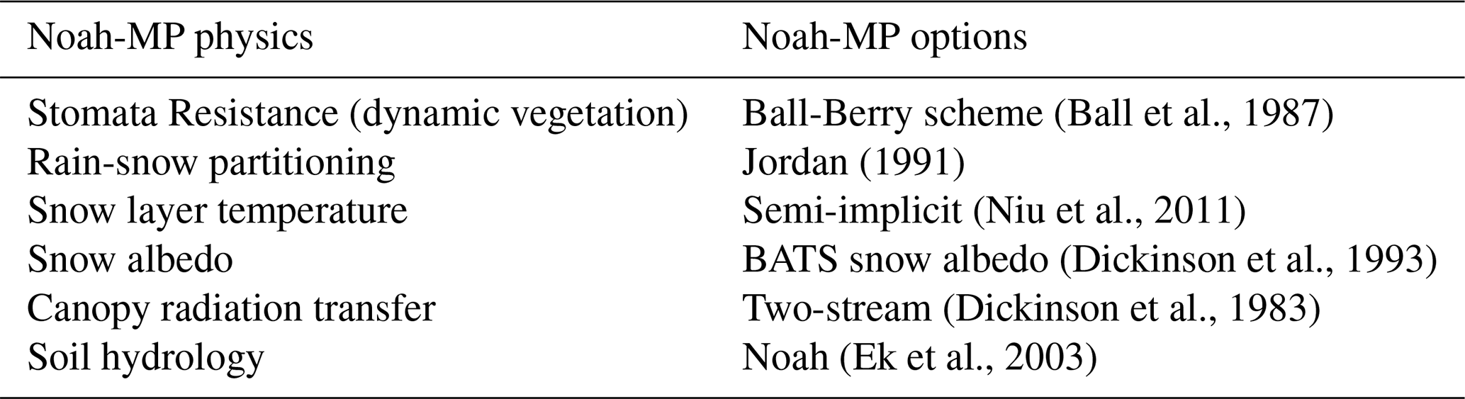
Noah-MP v5 was set up for the Sacramento and San Joaquin basins at 1 km spatial and hourly temporal resolution using hourly AORC v1.1 and downscaled NLDAS-2 forcing data. The Sacramento River Basin domain has 363 × 310 (south-north, west-east) grids and the San Joaquin domain has a 285 × 252 (south-north, west-east) grids. The simulation period is between 2015–2019 (5 years), and the model was spun up for a period of 5 years using the data of year 2014 (run the model for 5 cycles). We then use the restart file to run the model from 2015–2019. The model simulations were performed in Lambert Conformal Conic (LCC) projection consistent with the forcing data. The maximum soil depth was set to 2 m with 4 layers while the snowpack had up to three layers depending on snow depth. We selected two dynamic vegetation options (Table 1) including different combinations of LAI and GVF options. The prescribed monthly LAI climatology is from the Noah-MP lookup table for LAI, which were prescribed for a specific vegetation type based on global mean values. The prescribed GVF is assumed as a maximum yearly vegetation fraction. Combining the two basins, two forcing datasets, and two dynamic vegetation options, a total of 8 simulations were carried out in the study. Other key Noah-MP physics parameterizations related to snow–vegetation interactions are summarized in Table 2. These configurations define the representation of canopy processes, snow dynamics, and soil hydrology used in this study.

Table 1 Simulation acronyms and dynamic vegetation options used in the study.

Table 2 Noah-MP physics option used in the study related to snow-vegetation interaction.

5 Results

5.1 Meteorological Downscaling

The downscaled NLDAS-2 dataset shows more precipitation than does AORC, however, the daily mean aligns well with PRISM in the San Joaquin River Basin (Fig. 2). In particular, over higher altitudes, NLDAS-2 shows even more precipitation compared to AORC. Precipitation intensity is underestimated by AORC compared to PRISM and NLDAS-2 in both basins. In the Sacramento River Basin, the average daily PRISM precipitation is 2.7 mm (upper-left average values in Fig. 2), and the downscaled NLDAS-2 precipitation shows a higher magnitude (Fig. 2). However, AORC shows an underestimation of precipitation by a magnitude of 0.1 mm d⁻¹ averaged over the five-year period. More apparently, NLDAS-2 shows higher intensity precipitation especially over the Serra Nevada Mountain range (Fig. 2) than does the AORC forcing. Such discrepancies of AORC lead to underestimation of snow over the high mountains. Both AORC and NLDAS-2 precipitation data uses PRISM climatology as a reference; hence, their spatial precipitation patterns are quite similar. However, AORC underestimates the amount and intensity of precipitation when compared to PRISM and NLDAS-2 at higher elevations. Elevation dependent boxplots show that AORC constantly underestimates precipitation at all elevations, particularly at the highest elevation band (Fig. 2d). NLDAS-2 slightly underestimates the precipitation at lower elevations, however, it produces larger precipitation at high elevations where there is substantial snowfall. The precipitation from NLDAS-2 aligns quite well with PRISM between 1000 to 3000 m (Fig. 2d), and over this range it also agrees with the mean precipitation from the available GHCN and CDWR stations (CDWR stations represented with ^* in Fig. 2d, h), however the gauge undercatch, which is more serious for snowfall, is not corrected at the CDWR stations (as discussed later in the discussion section). GHCN stations are limited to lower altitudes but shows higher mean precipitation compared to any other gridded products in the Sacramento. However, R² values shows that GHCN stations are more aligned to AORC compared to NLDAS (Fig. S1 in the Supplement) because NLDAS are underestimated in lower altitudes compared to AORC.

In the San Joaquin River Basin, NLDAS-2 shows identical daily-mean precipitation (1.9 mm d⁻¹) as PRISM (Fig. 2e–g), while AORC shows a lower value (1.8 mm d⁻¹), ∼ 0.1 mm d⁻¹ less. As in the Sacramento River Basin, the downscaled NLDAS-2 and PRISM data also have similar spatial patterns (with comparable amounts), but AORC has too little precipitation in the mountainous areas in the San Joaquin River Basin.

Figure 2 The 1 km AORC and downscaled 1 km NLDAS-2 precipitation using WRF-Hydro MFE (mm d⁻¹) compared to the 4 km PRISM data over the Sacramento (upper panels, a–c) and San Joaquin River Basins (lower panels, e–g). Spatial daily mean has been annotated in the plot. Boxplot of these gridded products and GHCN stational observations (Fig. S1) over the two basins are plotted in (d) and (h), ^* represents the mean from the available CDWR stations in each River Basins (Fig. 1). Contour lines represent the elevation in the basins.

The downscaled temperature from NLDAS-2 shows a higher temperature in the valley regions and lower temperature in the mountain regions compared to AORC and PRISM (Fig. 3). The higher precipitation and lower temperature in NLDAS-2 favor snowfall and thus snow accumulation. In the Sacramento River Basin, the downscaled NLDAS-2 temperature is closer to the basin-averaged, daily mean temperature of PRISM. The daily mean temperature of PRISM is 286.7 K, whereas AORC and downscaled NLDAS-2 temperature are 286.3 K (0.4 K less) and 286.5 K (0.2 K less), respectively (Fig. 3a–c). The valley-mountain temperature difference is more noticeable in NLDAS-2 than AORC. Boxplots show that downscaled NLDAS-2 has colder temperatures compared to PRISM and AORC at higher elevations (> 2000 m), with warmer temperatures at lower elevations (< 1000 m) (Fig. 3d). The available CDWR stations (represented with ^* in Fig. 3d, h) also closely follows the gridded datasets. In the San Joaquin River Basin, the daily-mean temperature of PRISM is 287.5 K, which is better captured by AORC. However, NLDAS-2's temperature is higher by 0.8 K (Fig. 3e–g) and shows a stronger temperature gradient across the elevation compared to the other two datasets. Like the Sacramento River Basin, except the lower elevation (< 2000 m), NLDAS-2 produces colder temperature compared to PRISM, AORC, and available GHCN and CDWR stations (Fig. 3h). In the San Joaquin River Basin, R² values shows that GHCN station temperature are more aligned to AORC compared to NLDAS-2 (Fig. S1). The temperature downscaling based on the lapse rate provided by NCAR is sensitive to the altitudinal difference and thus causes the changes in the temperature gradient compared to PRISM.

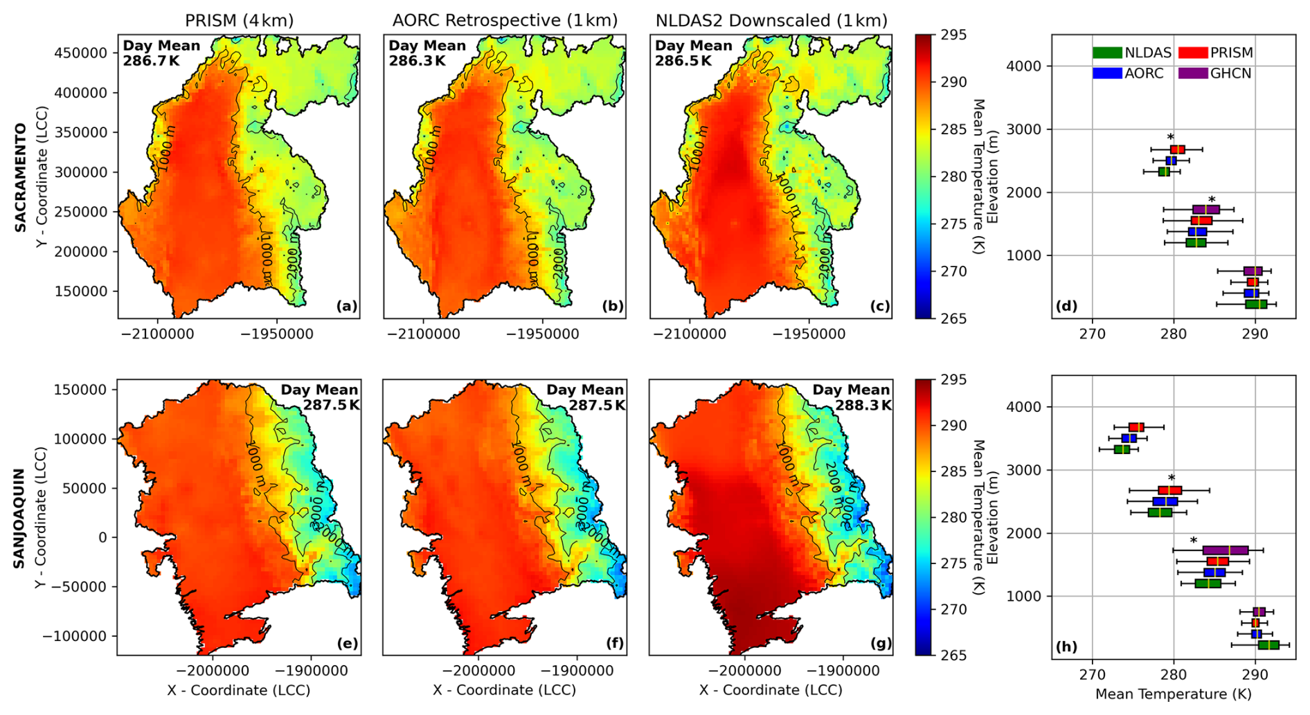
Figure 3 Downscaled 1 km AORC and NLDAS-2 temperature compared to the 4 km PRISM data using WRF-Hydro MFE over the Sacramento (upper panels, a–c) and San Joaquin River Basins (lower panels, e–g). Daily mean averaged over the basins is annotated in the plot. Boxplot of these gridded products and GHCN observation stations (Fig. S1) over the two River Basins are plotted in (d) and (h), ^* represents the mean from the available CDWR stations in each River Basin (Fig. 1). Contour lines represent the elevation in the basins.

5.1.1 SWE sensitivity to Precipitation Forcing and dynamic Vegetation

We first analysed the sensitivity of the modeled SWE to different precipitation data and vegetation conditions (Fig. 4). In both river basins, the downscaled NLDAS-2 forcing produces more SWE than AORC forcing by up to 100 mm in the peak SWE. NLDAS-2 produces more SWE than SNODAS, whereas the AORC produces less SWE than SNODAS under all vegetation conditions. In all cases, the dynamic vegetation module results in less accumulated SWE than the default, prescribed vegetation by 20–30 mm. In the Sacramento (Fig. 4a and b), the impact of vegetation on the annual cycle of SWE is more notable than in the San Joaquin Basin (Fig. 4c and d) due to the less coverage of broadleaf and needleleaf forests in the San Joaquin compared to the Sacramento (Fig. 1). The dynamic vegetation module produces better results (closer to SNODAS) when driven by the NLDAS-2 forcing but worse when driven by AORC in both basins. These simulations suggest that the modeled SWE are most sensitive to the choice of precipitation products followed by the choice of vegetation schemes.

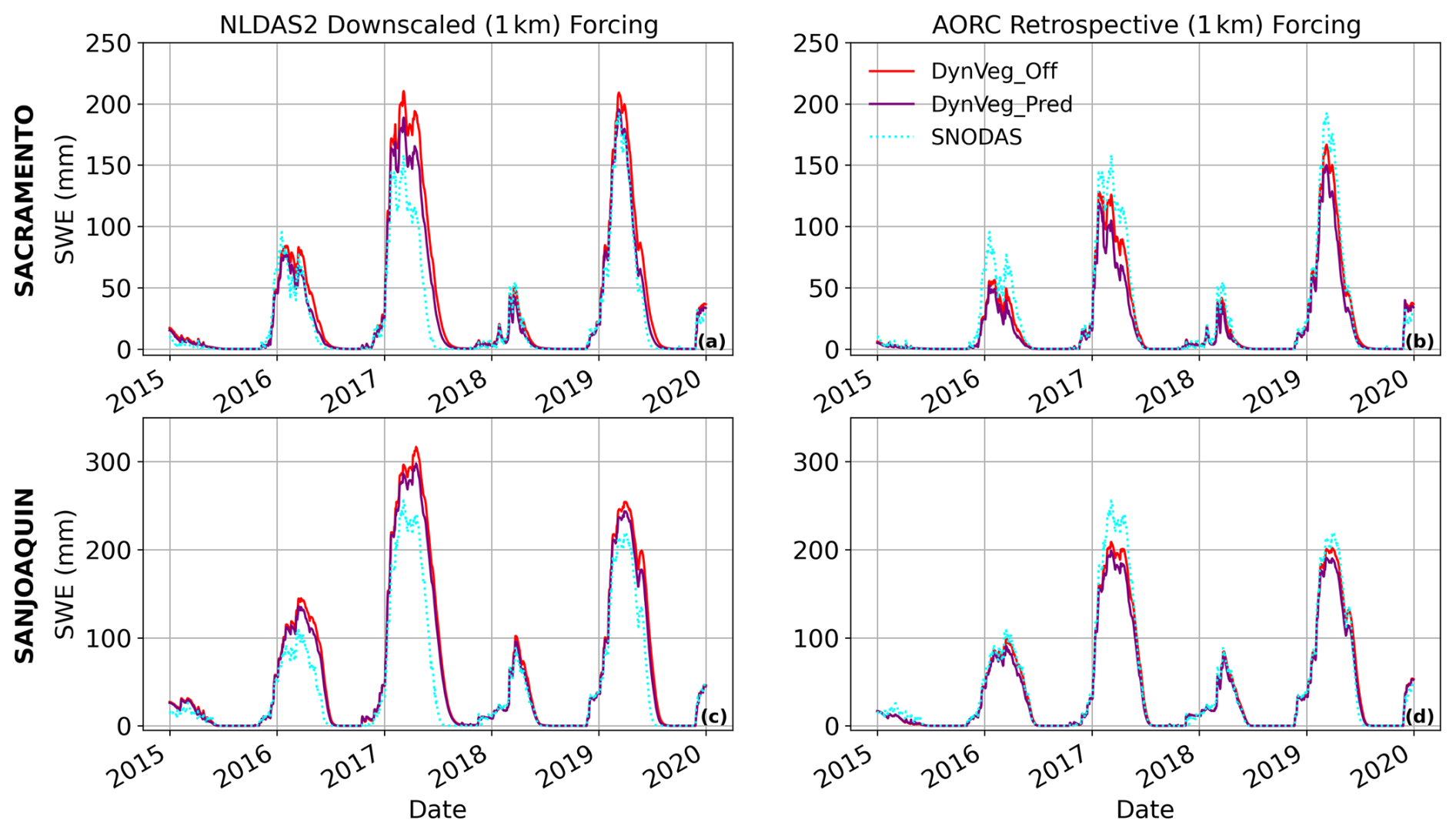
Figure 4 Modeled snow water equivalent (SWE) driven by different atmospheric forcing data (left panels: NLDAS-2; right panels: AORC) under the prescribed vegetation (DynVeg_Off) and dynamic vegetation (DynVeg_Pred) in the Sacramento (upper two panels) and San Joaquin (lower two panels) River Basins. Independent SWE estimates, SNODAS (1 km daily, Sect. 3.2), is also included.

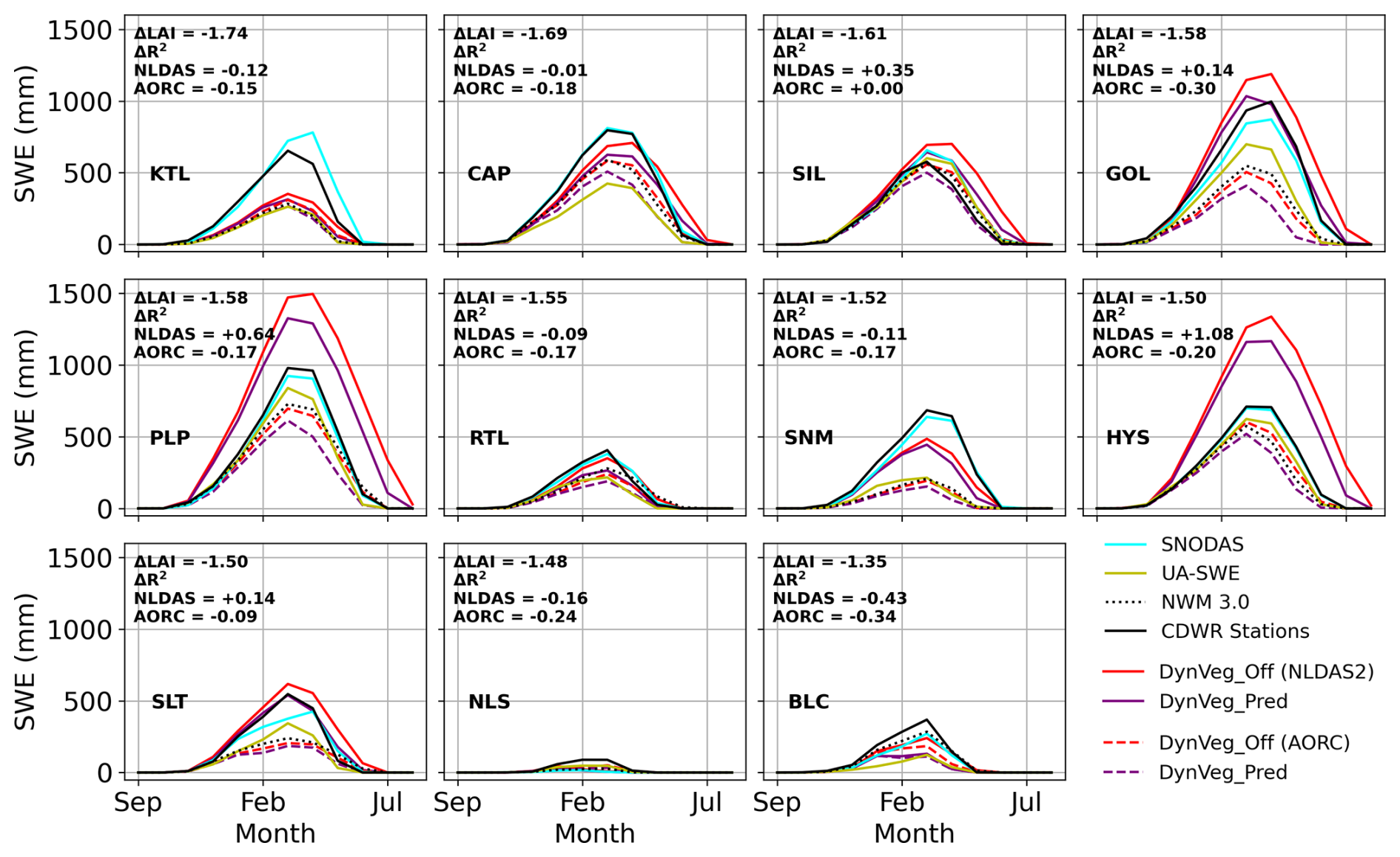
Figure 5 Snow water equivalent (SWE) comparison at CDWR stations in the Sacramento River Basin as represented in study area figure (Fig. 1). Monthly mean of control and dynamic vegetation modeled SWE with NLDAS-2 (solid lines) and AORC (dotted lines) forcing are plotted against the gridded observation (UA-SWE, SNODAS and NWM 3.0), and CDWR station (solid black line). The stations are sorted according to the difference in the LAI between both simulations, improvement in R² is also reported for each plot.

We have used 23 CDWR stations across the two river basins to evaluate the modeled SWE from different simulations. We show the results from all stations (Figs. 5, 6) to illustrate the impact of forcing and dynamic vegetation on SWE simulation. The stations in Figs. 5 and 6 are sorted according to the magnitude of the mean LAI difference (ΔLAI) between DynVeg_Pred and DynVeg_Off. The corresponding changes in R² ($\mathrm{\Delta }{R}^{\mathrm{2}}=R_{\mathrm{DynVeg}\mathrm{\_}\mathrm{Pred}}^{\mathrm{2}}-R_{\mathrm{DynVeg}\mathrm{\_}\mathrm{Off}}^{\mathrm{2}}$) are also reported for both NLDAS-2 and AORC forcing. Under NLDAS-2, several stations with substantial LAI changes show improved SWE performance, whereas similar LAI changes do not consistently improve under AORC. These station-scale differences indicate that the SWE response to dynamic vegetation is spatially heterogeneous and dependent on the meteorological forcing. For example, at GOL station, AORC produces less SWE when compared to CDWR (∼ 300 mm during peak SWE) under both vegetation conditions. The simulation with NLDAS-2 and prescribed vegetation (DynVeg_Off) produce much larger SWE, which lasts longer (Figs. 5, 6). The same simulation with dynamic vegetation (DynVeg_Pred) matches quite well with CDWR. The gridded SWE products also seem to be underestimated with SNODAS performing slightly better than UA-SWE and NWM 3.0. However, at a higher altitude the SWE difference becomes much larger. Here AORC simulations are underestimated by ∼ 500 mm during the peak SWE in March month over simulation period (Figs. 5, 6). The dynamic vegetation shortens the snow season compared to the simulation with prescribed LAI and matches well the observations. In general, except the GRM station (in the San Joaquin), NLDAS-2 forcing consistently produces better or comparable results (Table 3). GRM location shows low precipitation in PRISM and as well as downscaled NLDAS-2 (Fig. 2). It's highly likely that the low precipitation was inherited from the PRISM monthly climatology, this can be further investigated in the future work. The higher elevation stations (CAP, GNL, TUM and HHM) shows that NLDAS-2 with dynamic vegetation produce optimum snow amount. At 11 CDWR stations in the Sacramento and 12 CDWR stations in the San Joaquin, the model consistently performs better with NLDAS-2. This also supports daily SWE estimation in both river basins using NLDAS-2 (Fig. 4). The gridded UA-SWE and NWM 3.0 are underestimated, whereas SNODAS data are slightly better to match CDWR in terms of magnitude and seasonal cycle. The simulation with the prescribed vegetation shows a longer snow season than that of the gridded SNODAS data or CDWR. At the SLT, HYS, GOL, PLP, SIL, PSR, HNT, CHM, BLD, TMR, SLM, GNL and TUM station, NLDAS-2 downscaled forcing produces SWE better than AORC forcing (Table 3). In the lower altitude stations, NLDAS-2 SWE datasets are better than AORC, compared to CDWR. At the SLT, RBB, KIB, GOL, PSR, CAP and KSP stations, the simulations with the dynamic vegetation module capture the temporal variability better than its counterpart. Of particular interests, at the mid-altitude stations (HYS, GOL, PLP, PSR, CHM, BLD, TMR and SLM), there is a large difference between the simulations with and without the dynamic vegetation module because of the dominant broadleaf and needleleaf forests.

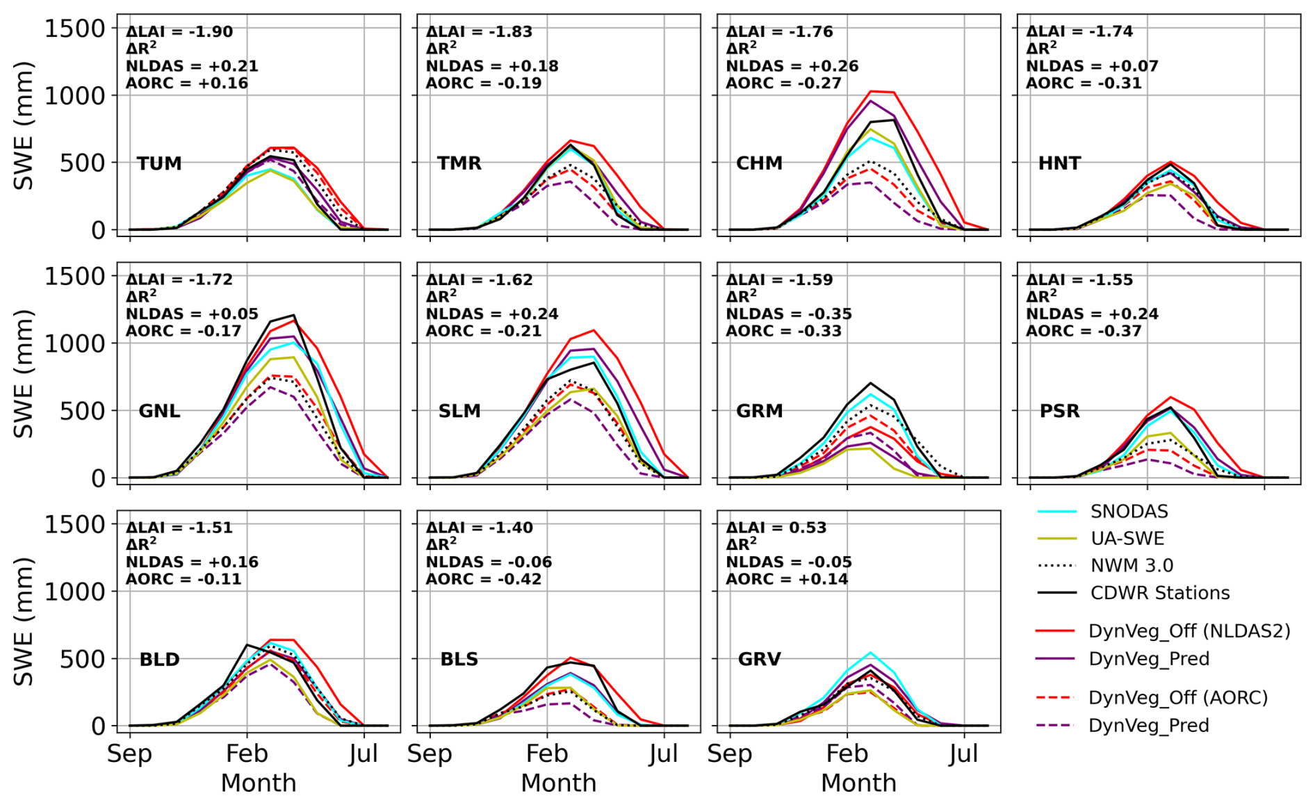
Figure 6 Snow water equivalent (SWE) comparison at CDWR stations in the San Joaquin River Basin as represented in study area figure (Fig. 1). Monthly mean of control and dynamic vegetation modeled SWE with NLDAS-2 (solid lines) and AORC (dotted lines) forcing are plotted against the gridded observation (UA-SWE, SNODAS and NWM 3.0), and CDWR station (solid black line). The stations are sorted according to the difference in the LAI between both simulations, improvement in R² is also reported for each plot.

Table 3 Statistical metrics for the SWE from 23 CDWR stations using NLDAS-2 and AORC atmospheric forcing datasets under the prescribed vegetation (DynVeg_Off) and dynamic vegetation (DynVeg_Pred) as shown in figure 5 and 6. Bold numbers shows improvement using dynamic vegetation model.

5.2 The Role of Vegetation Canopy

The difference between simulations with and without dynamic vegetation is the prediction of LAI. In both the river basins, the prescribed LAI (DynVeg_Off) is much higher than the predicted LAI (DynVeg_Pred) across almost all altitudes (Fig. 7). The prescribed LAI also shows less seasonality compared to the predicted LAI. The prescribed LAI values in DJF and MAM are higher than the MODIS LAI above 1000 m (Fig. 7a–b). The simulations with the dynamic vegetation module produce LAI values closer to the MODIS LAI, especially in DJF at higher altitudes. Another independent LAI product from Sun Yat-sen University suggests slightly closer agreement with the dynamic vegetation simulation. The LAI values in DJF and MAM show that the dynamic vegetation model shows a capability of simulating the seasonal and altitudinal variability in LAI. Note that the prescribed LAI values (from Noah-MP parameters table) correspond to those used in NWM which affects the SWE dynamics in a similar manner (Johnson et al., 2023). The simulation driven by AORC produces slightly higher LAI compared to that by NLDAS-2 at higher altitudes (Fig. 7c–d) due possibly to the warmer temperatures of AORC (Fig. 3d). The model predicted LAI can be further improved if the parameters controlling the leaf dynamics (e.g., the type-dependent specific leaf area, m² kg⁻¹ C) are further optimized.

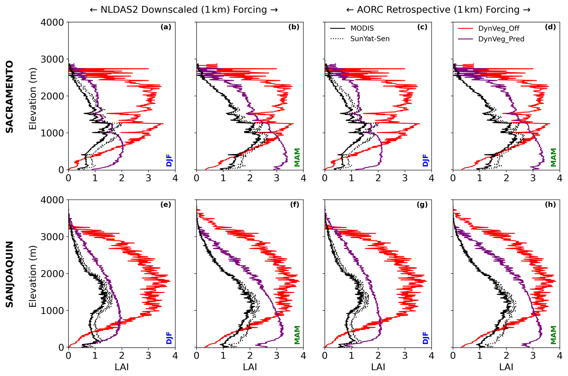
Figure 7 Altitudinal variation of the modeled leaf area index (LAI) for two seasons (winter: DJF, spring: MAM) using different atmospheric forcing data (two left panels: NLDAS-2; two right panels: AORC) under prescribed vegetation (DynVeg_Off) and dynamic vegetation (DynVeg_Pred) in the Sacramento (upper panel) and San Joaquin (lower panel) River Basins. Independent LAI estimates from the MODIS and Sun Yat-sen University are also included.

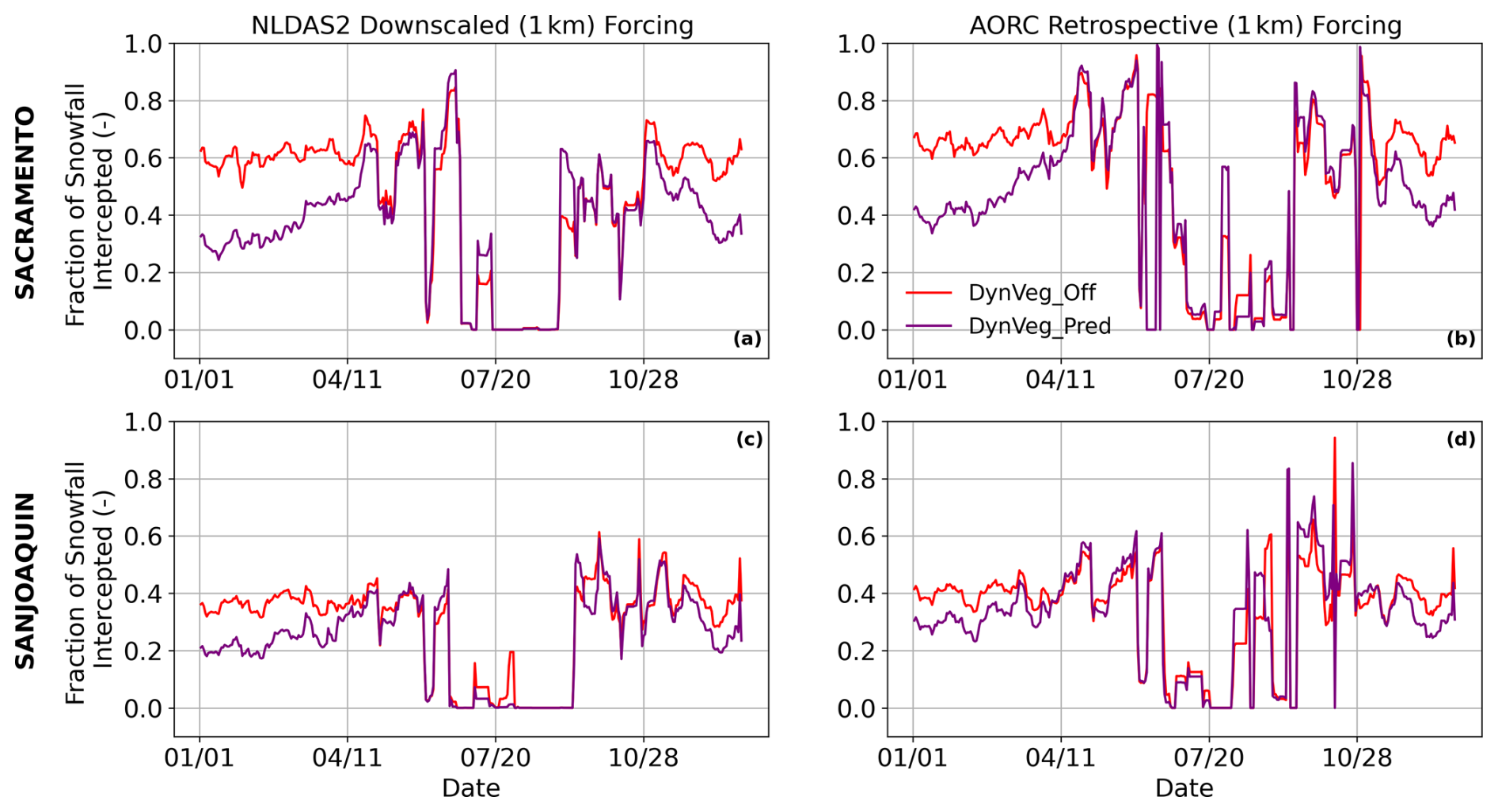
Figure 8 Modeled (normalised) canopy intercepted snow rate using different atmospheric forcing data (left panels: NLDAS-2; right panels: AORC) under prescribed vegetation (DynVeg_Off) and dynamic vegetation (DynVeg_Pred) in the Sacramento (upper two panels) and San Joaquin (lower two panels) River Basins. The intercepted snow was normalised using the snowfall from each forcing datasets. A SWE threshold of 0.1 mm has been applied to mask the region and perform spatial average.

Vegetation conditions directly impact the snow dynamics beneath the canopy through interception/sublimation of snow and changes in the energy budgets on the snow surface. The canopy intercepted snow resulting from DynVeg_Off is higher than DynVeg_Pred in both basins due to the larger prescribed LAI and GVF (Figs. S2 and S3) in DynVeg_Off (Fig. 8, Table 4). The canopy intercepted snow is higher during the accumulation period and then decreases as snowfall decreases in the melting season. Driven by AORC, the canopy intercepted snow is slightly smaller than that by NLDAS-2 (Fig. 8) due to the less snowfall (as a result of the less precipitation and warmer temperature). Table 4 presents the mean daily snowfall (SNOW) and canopy-intercepted snow rate (ICEPT) across the Sacramento and San Joaquin River Basins for different forcing datasets and vegetation configurations. While snowfall remains largely unchanged between prescribed and dynamic vegetation, canopy interception is consistently reduced under dynamic vegetation, with variations across datasets and basins. In the San Joaquin River, as the canopy density (LAI) is less than in the Sacramento, the differences in the canopy intercepted snow between the two experiments are less compared to the Sacramento River (Fig. 8c and d, Table 4). In general, the dynamic vegetation produces a lower ratio of canopy interception to actual snowfall, depending on LAI and vegetation cover fraction (GVF) (Table 4).

Table 4 Daily snowfall (SNOW) and daily canopy intercepted snow rate (ICEPT) for the different forcing datasets (NLDAS-2, AORC) under prescribed vegetation (DynVeg_Off) and dynamic vegetation (DynVeg_Pred) in Sacramento and San Joaquin River Basins. The table has been shown for the masked region similar to Fig. 7.

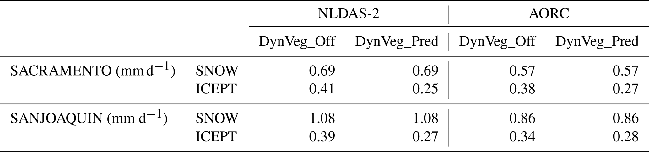
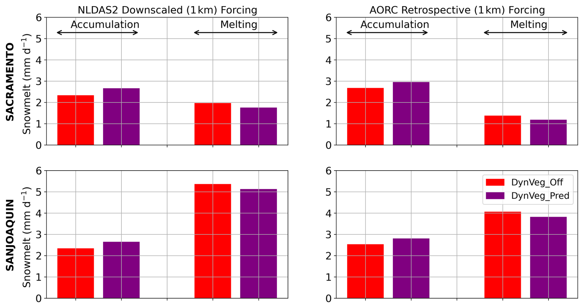
Figure 9 Modeled snowmelt rate (daily) during accumulation (DJFM) and melting (AMJJ) seasons using different atmospheric forcing data (left panels: NLDAS-2; right panels: AORC) under prescribed vegetation (DynVeg_Off) and dynamic vegetation (DynVeg_Pred) in the Sacramento (upper two panels) and San Joaquin (lower two panels) River Basins. A SWE threshold of > 0.1 mm has been applied to mask the region and perform spatial average.

The vegetation canopy with intercepted snow can substantially modify the energy budgets of the snow surface beneath the canopy and hence snowmelt and sublimation (Figs. 9, S4). Unlike high-latitude regions, there are substantial episodic snowmelt occurring in the accumulation in these subtropical mountains. Driven by both forcing datasets (NLDAS-2 and AORC), the snowmelt rate in both river basins resulting from DynVeg_Off shows a lower melting rate by up to 0.2 mm d⁻¹ during the accumulation period (DJMF), resulting in the larger peak SWE resulting from DynVeg_Off (Fig. 4). Later in the melting the season (AMJJ), the snowmelt rate from DynVeg_Off exceeds that from DynVeg_Pred due mainly to the changes in solar radiation received by the snow surface (Fig. 10; will be discussed further).

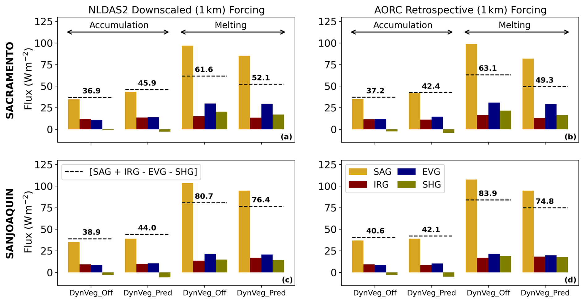
Figure 10 Modeled snow surface energy fluxes averaged over the accumulation (DJFM) and melting snow season (AMJJ) driven by different atmospheric forcing data (left panels: NLDAS-2; right panels: AORC) under prescribed vegetation (DynVeg_Off) and dynamic vegetation (DynVeg_Pred) in the Sacramento (upper two panels) and San Joaquin (lower two panels) River Basins. Acronyms correspond to net shortwave radiation (SAG), net longwave radiation (IRG), latent heat (EVG) and sensible heat (SHG) at the snow surface. The net budget is plotted as dashed lines and corresponding value is written on the top of the dashed lines. A SWE threshold of 0.1 mm has been applied to mask the region and perform spatial average.

To disentangle the dominate control of snowmelt rate, we separately explored the below-canopy energy fluxes including the net shortwave radiation (SAG), net longwave radiation (IRG), latent heat (EVG) and sensible heat (SHG) fluxes at the snow surface during the accumulation (DJFM) and melting (AMJJ) seasons (Fig. 10). In Noah-MP, the energy available for snowmelt is controlled by the snow surface energy balance: SAG + IRG − EVG − SHG (Wm⁻²). It turns out that the net solar radiation (received by the snow surface) is much larger than other energy balance components in all cases for both accumulation and meting season (Fig. 10). During the accumulation period (DJFM), the higher LAI in DynVeg_Off reduces the shortwave radiation reaching the snow surface due mainly to the canopy shading effect, which is highly dependent on vegetation density (LAI and GVF) and solar angle. In contrast, during the melting season (AMJJ), GVF in DynVeg_Pred exceeds that in DynVeg_Off, leading to stronger shading despite the consistently higher LAI in DynVeg_Off (Figs. S2 and S3). As solar elevation increases (the Sun is more overhead), the shading effect becomes more sensitive to GVF than LAI, resulting in reduced snowmelt energy in DynVeg_Pred compared to DynVeg_Off. Although other energy fluxes also increase during the melting season, their differences between the two experiments are relatively small compared to the impact of canopy shading.

6 Discussion

We have shown the capability of dynamic vegetation module to simulate LAI and how it can impact the snowpack dynamics through processes of snow interception and canopy shading. Such impacts can result in longer snowmelt, altering soil moisture, and partitioning of hydrological fluxes. Snow-vegetation interaction is complex yet intriguing in nature. Chen et al. (2014) highlighted the importance of forcing and model physics in perturbing the below canopy radiation budget however, they cannot explain the canopy shading effect. The canopy shading decreases the solar energy reaching the ground snow, which results in less episodic snowmelt during the accumulation season and more SWE. This kind of impact can only be observed with the more accurate estimation of LAI, which is achieved with the dynamic vegetation module. With limited gridded estimates, we have shown that dynamic vegetation produces improved LAI estimates, which can influence the simulated SWE dynamics. For the simulation purpose, we have used two kinds of forcing datasets AORC and NLDAS-2. AORC forcing is a well-known dataset for calibrating hydrological models over CONUS (Cosgrove et al., 2024; Kitzmiller et al., 2018). We have used the mountain mapper algorithm (one of the method used in generating AORC datasets) to downscale the NLDAS-2 datasets. In our study regions in California, we found that AORC is underestimated compared to PRISM and the downscaled NLDAS-2. Hence, the modelled SWE with the AORC forcing is underestimated compared to the gridded estimates and more significantly when compared to the 23 CDWR stational data over the mountains. Many studies have suggested that the operational NWM, which uses the same forcing (AORC) generally underestimated the peak SWE in the Western United States (Garousi-Nejad and Tarboton, 2022; Yang et al., 2022, 2023). This study also indicates that using AORC, the model underestimates SWE in lower and mid-elevation stations (Sect. 5.2) in consistent with Yang et al. (2022).

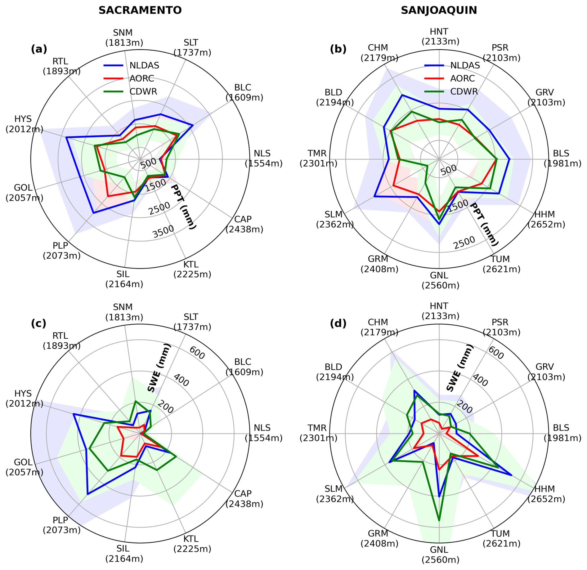
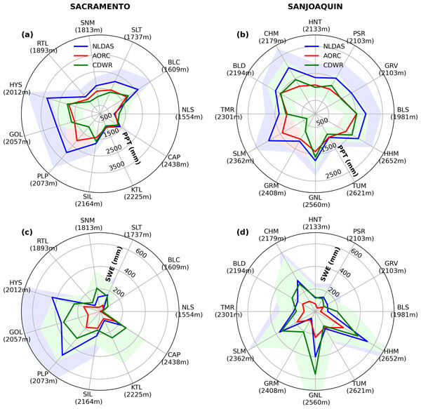
Figure 11 Comparison of yearly mean precipitation (a, b) and SWE (c, d) data from NLDAS-2 and AORC against the CDWR stational data (left panels: 11 stations in Sacramento River Basin; right panels: 12 stations in the San Joaquin River Basin). The modeled SWE data are taken from the DynVeg_Pred simulation. The shaded region represents the standard deviation of the datasets across 5 years at each station. The CDWR precipitation data are not corrected for gage undercatch.

Dynamic vegetation mainly simulates the LAI and GVF through the carbon budgets of plants' photosynthesis and respiration (Niu et al., 2011). Having more accurate LAI helps improve the snow on the ground, canopy interception of snow, radiation transfer and canopy evaporation/sublimation (Hedstrom and Pomeroy, 1998; Moeser et al., 2015). The chosen dynamic vegetation method outperform the prescribed LAI (Sect. 5.3). This enhances the SWE simulations across elevation. We have shown that NLDAS-2 produces more precipitation (closer to PRISM) compared to AORC. However, when we compared the gridded precipitation to the CDWR station observation, we have found that AORC matches quite well CDWR stations (Fig. 11a, b). This comparison is contrary to the SWE datasets from same stations, which shows a more comparable SWE to NLDAS-2 forcing and severe underestimated SWE with AORC forcing (Fig. 11c, d). These contrasting results can be largely attributed to limitations in the observational datasets. In particular, the CDWR precipitation measurements are not corrected for gauge undercatch, which can lead to systematic underestimation of snowfall (Lundquist et al., 2015). In contrast, the gridded SWE products, SNODAS and UA-SWE, are derived using data assimilation and machine learning approaches, respectively, and incorporate multiple in situ SWE or snow depth observations. Relative to these gridded datasets, the NLDAS-2 driven simulations tend to overestimate SWE, whereas simulations forced by AORC exhibit a clear underestimation. Moreover, CDWR stations are often preferentially located in areas with deeper snowpacks, potentially influenced by wind driven snow redistribution, which introduces a positive bias when extrapolating point-scale observations to the 1 km model grid. Given these representativeness issues, simulations forced by NLDAS-2 with prescribed vegetation parameters (LAI and GVF) substantially overestimate SWE, while the inclusion of a dynamic vegetation module yields more realistic SWE estimates that better align with SNODAS. Nevertheless, even with dynamic vegetation, the NLDAS-2 forced simulations still produce higher SWE than SNODAS, likely because the modeled LAI remains larger than that derived from MODIS observations.

This study highlights the importance of accurately representing fine-scale vegetation processes in large-scale hydrological and land surface models, demonstrating that subgrid vegetation heterogeneity can substantially alter simulated hydrological behavior. In particular, under- or over-representation of leaf area index (LAI) at the subgrid scale can significantly influence the diurnal dynamics of energy partitioning, snow accumulation and runoff generation by modulating canopy interception, radiation transfer, and snow–vegetation interactions. These findings suggest that commonly used grid-averaged vegetation parameterizations may obscure critical nonlinear responses in snow accumulation and melt processes. Future land surface modeling efforts should therefore explicitly investigate the role of subgrid vegetation structure and phenology to reduce uncertainties in regional- to global-scale snow and hydrologic simulations. Because LAI directly affects both snow accumulation and ablation through canopy shading, longwave enhancement, and interception processes, it also controls snow persistence and seasonal snow cover duration. Changes in snow cover duration can, in turn, modify surface albedo and land–atmosphere energy exchanges, potentially affecting regional atmospheric feedback (He et al., 2021; Lee et al., 2024). Incorporating these mechanisms offers a promising pathway toward more physically consistent coupled land–atmosphere modeling frameworks.

7 Summary

Most hydrological models and LSMs, e.g., NWM (Garousi-Nejad and Tarboton, 2022), CLM v4.0 (Toure et al., 2016), Noah-MP and other LSMs (Cho et al., 2022) significantly underestimate SWE, which is a major source of water to fill the surface reservoirs and recharge groundwater in the dry western US, and so do various global reanalyses like ERA, ERA-Land, MERRA-2 and GLDAS (Broxton et al., 2016). This modelling study in the Sacramento and San Joaquin River basins in California suggests that

1. The Noah-MP predicted SWE is most sensitive to the high-resolution (1 km) precipitation inputs compared to other process representations, e.g., the vegetation dynamics. The use of the 1 km downscaled NLDAS-2 produces substantially more SWE than using AORC and NWM 3.0 (which also uses AORC), especially at higher altitudes. This is favorable when compared to the CDWR stational data and other gridded products, e.g., SNODAS and UA SWE.

2. Following the precipitation inputs, the modeled SWE is also sensitive to the representations of vegetation dynamics. With the dynamic vegetation module, Noah-MP produces less SWE due mainly to the lower predicted LAI than the prescribed. This is favorable when the model is driven by the downscaled NLDAS-2 forcing. The lower predicted LAI may lead to less canopy interception of snowfall, resulting more SWE on the ground, but less significant shading effects, resulting in more shortwave radiation received by the snowpack beneath the canopy and thus more episodic snowmelt in the accumulation season. The overall shading effect appears to be greater than the interception effects, so the snowpack on the ground tends to be thinner and persist shorter when there is less vegetation canopies. The modeled LAI matches MODIS LAI better than does the prescribed but still higher than the MODIS LAI. Further calibration of vegetation parameters may result in lower LAI, which are preferable to produce less SWE and thus match the gridded SWE products (SNODAS and UA-SWE).

These findings highlight the importance of downscaling of atmospheric forcing and vegetation effects to the accuracy of snow modeling. Mountain mapper based NLDAS-2 downscaled data along with better representations of LAI and vegetation cover fraction can further improve snow predictions in the snow dominated river basins within NWM framework. The forthcoming dynamically downscaled NLDAS-2 dataset at 1 km resolution (NLDAS-3) has the potential to improve snow simulations in the western United States and merits further evaluation.