Seasonal surface melt onset and firn freeze-up across the central Wrangell and St. Elias Mountains

High-elevation alpine firn is increasingly influenced by surface melt and meltwater retention, yet the spatial extent and timing of these processes remain poorly quantified. Here, we use surface melt onset and firn freeze-up dates derived from Sentinel-1 C-band Synthetic Aperture Radar data from 2015–2024 to map dry firn and hydrologic transition zones, where firn is at a transition between dry and wet regimes, across the central Wrangell/St. Elias Mountains. Melt onset and freeze-up are identified from characteristic changes in backscatter associated with the presence of liquid water in snow and firn. Seasonal melt is detected across nearly all elevations in the range (0–5,670 m a.s.l.). Melt onset broadly tracks the seasonal rise of the 0 °C isotherm up to ∼ 3000 m a.s.l., while freeze-up shows pronounced delays relative to subfreezing air temperatures at mid-elevations (2000–3000 m a.s.l.), indicating widespread meltwater retention within the firn. We find that dry firn covers only 3 % of our study domain's glacierized area, while hydrologic transition zones cover 9 % of our study domain's glacierized area. Our results highlight the pervasive influence of meltwater retention on firn hydrologic regimes in the Wrangell/St. Elias Mountains and demonstrate the utility of Sentinel-1 SAR for mapping firn water retention and monitoring changes in regional firn hydrology in data-sparse mountain regions.

1 Introduction

Firn – snow that has survived at least one melt season – represents an intermediate stage in the transformation of new snow into glacial ice on glaciers and ice sheets worldwide (Miller, 1952). A healthy firn pack is essential for maintaining glacier mass balance; however, increasing evidence indicates that firn is warming and melting across many glacierized regions (Bezeau et al., 2013; Polashenski et al., 2014; Noël et al., 2018; Vandecrux et al., 2020; Ochwat et al., 2021; Horlings et al., 2022; Kindstedt et al., 2025).

Firn warming can modify its physical structure, thermal regime, and chemistry, thereby altering the thermal and chemical characteristics of developing glacier ice and compromising the climate records archived within (Samimi and Marshall, 2017; Ochwat et al., 2021; Kindstedt et al., 2025). In addition, porous firn can act as a buffer to glacier runoff, delaying the transfer of meltwater to downstream hydrological systems by years to decades in some regions (Harper et al., 2012; Koenig et al., 2014; Noël et al., 2018; MacFerrin et al., 2019; Culberg et al., 2021). When surface meltwater is retained within the firn pack as a firn aquifer, it may be stored for several years, further warming the firn while delaying runoff (Fountain, 1989; Schneider, 1999; Jansson et al., 2003; Miège et al., 2016; Ochwat et al., 2021). Conversely, near-surface refreezing of meltwater into ice layers can reduce firn permeability and increase runoff as a result of this fundamental change to firn structure (Machguth et al., 2016; MacFerrin et al., 2019). The presence of liquid water within snow and firn can also inhibit drilling access to underlying ice, complicating the recovery of preserved climate records. In short, crossing the cold-to-temperate firn threshold shifts firn evolution from dry densification to meltwater-driven processes, fundamentally altering glacier ice development, hydrologic buffering, and the preservation and recovery of ice core climate records.

Net firn warming over the course of a year occurs when the energy transferred into the firn during the melt season exceeds the regeneration of cold content during the winter, with cold content referring to the amount of energy required to raise the temperature of a given volume of firn to 0 °C (Vandecrux et al., 2020). When the snow surface is warmer than the firn column beneath (e.g. during the summer melt season), energy is transferred to the subsurface via conduction and meltwater percolation. In particular, the release of latent heat associated with subsurface refreezing of meltwater is a dominant factor in downward heat transport through snow and firn (Cuffey and Paterson, 2010).

While surface energy balance modeling provides the most complete framework for quantifying heat transfer and melt processes, its application at regional scales is often limited by the availability of distributed meteorological forcing and surface property data. Consequently, air temperature is often used as a first-order proxy for melt occurrence in glacierized regions (Hock, 2003). However, air temperature alone provides an incomplete proxy for firn thermal evolution, as it does not capture the spatial and temporal variability of meltwater production, percolation, and refreezing that dominate firn heat transfer. Whether firn remains cold or transitions toward temperate conditions depends not only on melt season surface temperature, but also on the subsurface retention of liquid water into the fall and winter, which, through latent heat release, reduces the efficiency of wintertime cold content regeneration.

The Wrangell and St. Elias Mountains (henceforth “Wrangell/St. Elias”) are extensively glacierized mountain ranges located on the border of Alaska and southwest Yukon (Fig. 1). High annual snow accumulation that insulates underlying firn (Marcus and Ragle, 1970), together with amplified high-elevation warming (Williamson et al., 2020) make Wrangell/St. Elias susceptible to increasing firn meltwater retention and aquifer development. While recent observations from Wrangell/St. Elias have shown evidence of firn warming and increased surface melt production and percolation (Ochwat et al., 2021; Kindstedt et al., 2025) and regional assessments have linked temperature to rising snowlines and melt extents (Bevington and Menounos, 2025; Wells et al., 2026), the spatial extent of firn transitioning from dry to wet conditions in Wrangell/St. Elias remains poorly constrained. Here, we use surface melt onset and firn freeze-up dates derived from Sentinel-1 SAR observations to map the distribution of firn hydrological transition zones across central Wrangell/St. Elias over a ten-year period (2015–2024).

2 Methods

2.1 Region of Study

We focus our analyses on the central Wrangell/St. Elias Mountains, and define our study domain as the area from 59.7586 to 61.4825° N and 137.8171 to 142.0295° W (45 470 km², 0–5959 m a.s.l., Fig. 1). Rising over 5000 m from sea level within 100 km of the coast, Wrangell/St. Elias represents one of the most dramatic barriers to inland transport of coastal moisture on the planet (Newman et al., 2020). Orographic precipitation resulting from this topography (mean 0.59 $\mathrm{m}\mathrm{w}.\mathrm{e}.{\mathrm{a}}^{-\mathrm{1}}$ at the Kaskawulsh/Hubbard Divide; Fig. 1; Kindstedt et al., 2026) sustains the extensive glaciers and icefields found in the range. We define our study domain to include the most heavily glaciated central Wrangell/St. Elias, characterized by interconnected glaciers and broad icefields rather than isolated small alpine glaciers. Fifty-one percent (23 190 km²) of the land surface area in our study domain is ice-covered, and feeds two of the largest watersheds (by discharge) that drain into the Gulf of Alaska: the Copper and the Alsek Rivers (Sergeant et al., 2020). The remainder of the land surface within our study domain is a mix of ocean, coastal plain, interior forest, waterways, and steep rocky slopes.

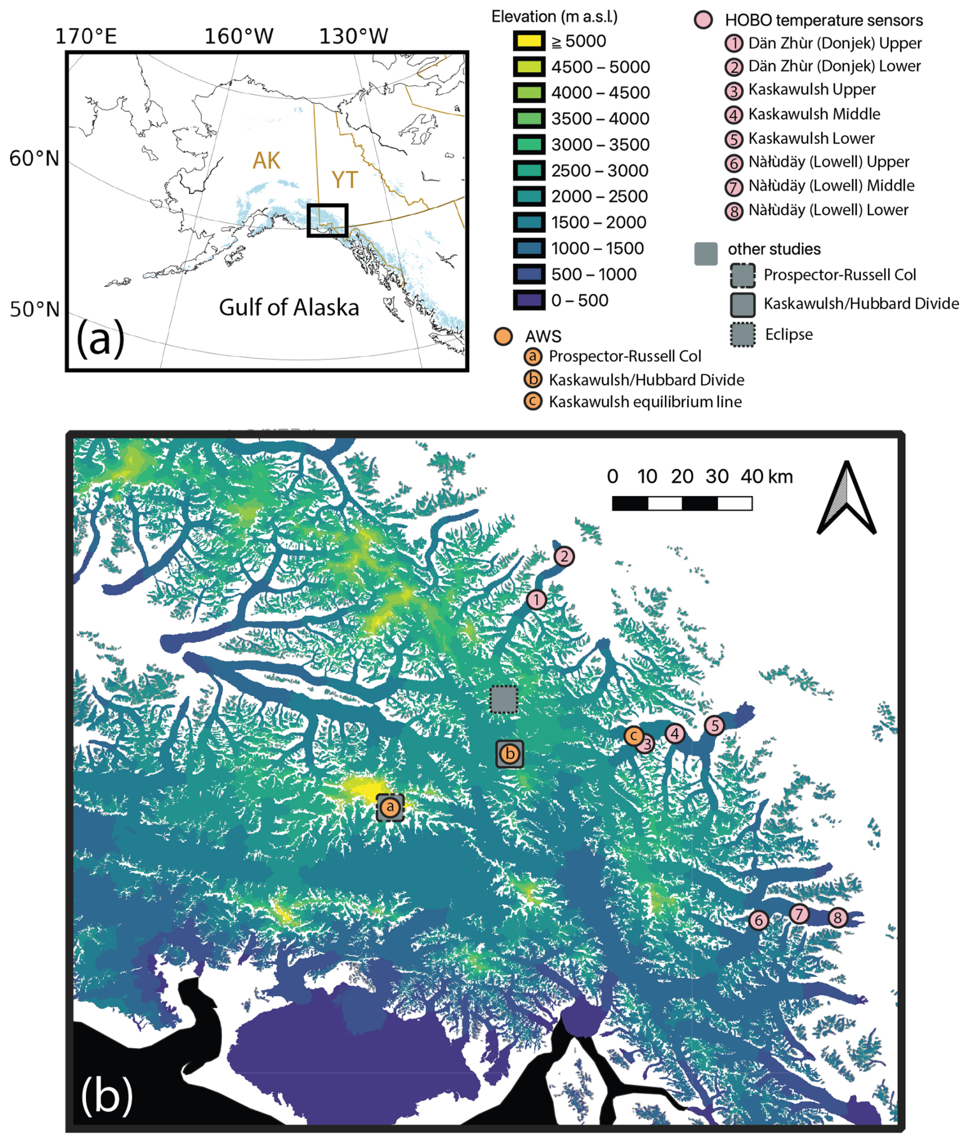
Figure 1 Study domain across Alaska (AK) and Yukon (YT) with digital elevation map (DEM) and ground-truth sites. A regional overview map is shown in panel (a) with the study domain indicated by the black rectangle. Binned land-surface elevations and ground-truth sites (colored circles and gray squares) across the study domain are shown in panel (b). The Gulf of Alaska is shown in black in panel (b).

2.2 Sentinel-1 Synthetic Aperture Radar (SAR) satellite imagery

To identify the onset and extent of surface melt in Wrangell/St. Elias, we utilize the drop in C-band SAR backscatter associated with the introduction of liquid water to a snowpack (Nagler and Rott, 2000; Nagler et al., 2016; Tsai et al., 2019). C-band SAR is an active microwave remote sensing technique that transmits radar pulses and measures the energy scattered back from the surface, making it sensitive to snow structure and dielectric properties. C-Band SAR is able to operate at night and through cloud cover, and is very strongly attenuated by water, providing a clear signal of melt onset despite dark or overcast conditions. In particular, we use backscatter measured by the Sentinel-1 mission in the interferometric wide beam mode because of its ability to produce imagery at sub-weekly temporal resolution (6 d revisit time) and high spatial resolution (20 m) across a 250 km wide swath. In addition, the operational wavelengths (centered at 5.56 cm) of Sentinel-1 are two orders of magnitude larger than typical snow grain sizes (0.1–0.3 mm; Tsai et al., 2019). Therefore, although grain size can affect SAR backscatter, it has a negligible influence on Sentinel-1 data. We use Sentinel-1 scenes in co-polarization (VV) because it is more sensitive to surface conditions, whereas cross-polarization (VH) is more strongly influenced by volume scattering within the snowpack (Lievens et al., 2019).

To avoid inconsistencies in backscatter associated with differences in satellite incidence angle among paths/frames, we identify melt onset and freeze-up dates independently for each path/frame. For pixels covered by multiple paths/frames, we assign the earliest detected date as the melt onset or freeze-up date. We use the term pixel as it is commonly used in SAR literature to refer to a single unit of gridded remote sensing data, rather than a picture element on a computer screen. We only use path/frames from descending Sentinel-1 orbits, which are acquired before 10:00 local time, to eliminate biased earlier melt detection for pixels with afternoon image acquisitions (all scenes in our study area are acquired before 10:00 or after 18:00). Sentinel-1 path/frames and scenes used in this study are provided in Appendix A.

Our analysis spans the 2015–2024 melt seasons, beginning with the launch of the first Sentinel satellite (Sentinel-1a) in 2014 (12 d revisit) and then including the addition of Sentinel-1b data from 2017 through 2022 (resulting in a 6 d revisit time). Gaps in available Sentinel-1 data temporarily reduce the temporal resolution of our timeseries and are addressed within our uncertainty calculations (Sect. 2.3).

2.3 Melt classification

Rather than directly measuring liquid water, the SAR-based melt detection method we use relies on the contrast between dry snow and melting snow backscatter values. Following Scher et al. (2021) and Nagler and Rott (2000), we use a timeseries of backscatter values from each pixel to classify that pixel as either dry or melting at the time of acquisition. A schematic of our melt classification method is shown in Fig. 2. Because melt is identified individually for each pixel relative to its dry-snow backscatter value, we first produce a reference dry-snow image from at least four wintertime (November–March) scenes. Pixels are classified as melting when their backscatter value is >3 dB lower than their dry-snow average (Nagler and Rott, 2000); otherwise, pixels are classified as dry.

To establish melt onset each year, we identify the first of at least two consecutive melting scenes in each pixel's backscatter timeseries and set melt as the date of image acquisition. We consider the uncertainty in melt onset date to be the number of days passed since the last dry Sentinel-1 observation before onset. We exclude pixels where melt onset is identified to be later than day 244 (1 September in non-leap years).

We identify freeze-up, or refreezing of the snow and firn, as the first of at least two consecutive dry scenes following a period of seasonal melting. The penetration depth of C-band SAR in wet snow (e.g. during the summer melt season) is only a few centimeters; however, as the snow and firn refreeze, Sentinel-1 can penetrate meters to tens of meters (Baghdadi et al., 1997; Tsai et al., 2019). Freeze-up timing inferred from increases in SAR backscatter may therefore reflect multiple processes, including surface refreezing, drainage, and firn structural change. As such, we use the term freeze-up to represent an integrated firn column response to changes in structure and liquid water content rather than a discrete physical threshold in surface conditions. We define the uncertainty in freeze-up date as the number of days elapsed since the last melting Sentinel-1 observation prior to freeze-up. When averaging melt onset or freeze-up date over multiple years, we consider the associated uncertainty (in days) to be the maximum uncertainty value among the individual years averaged.

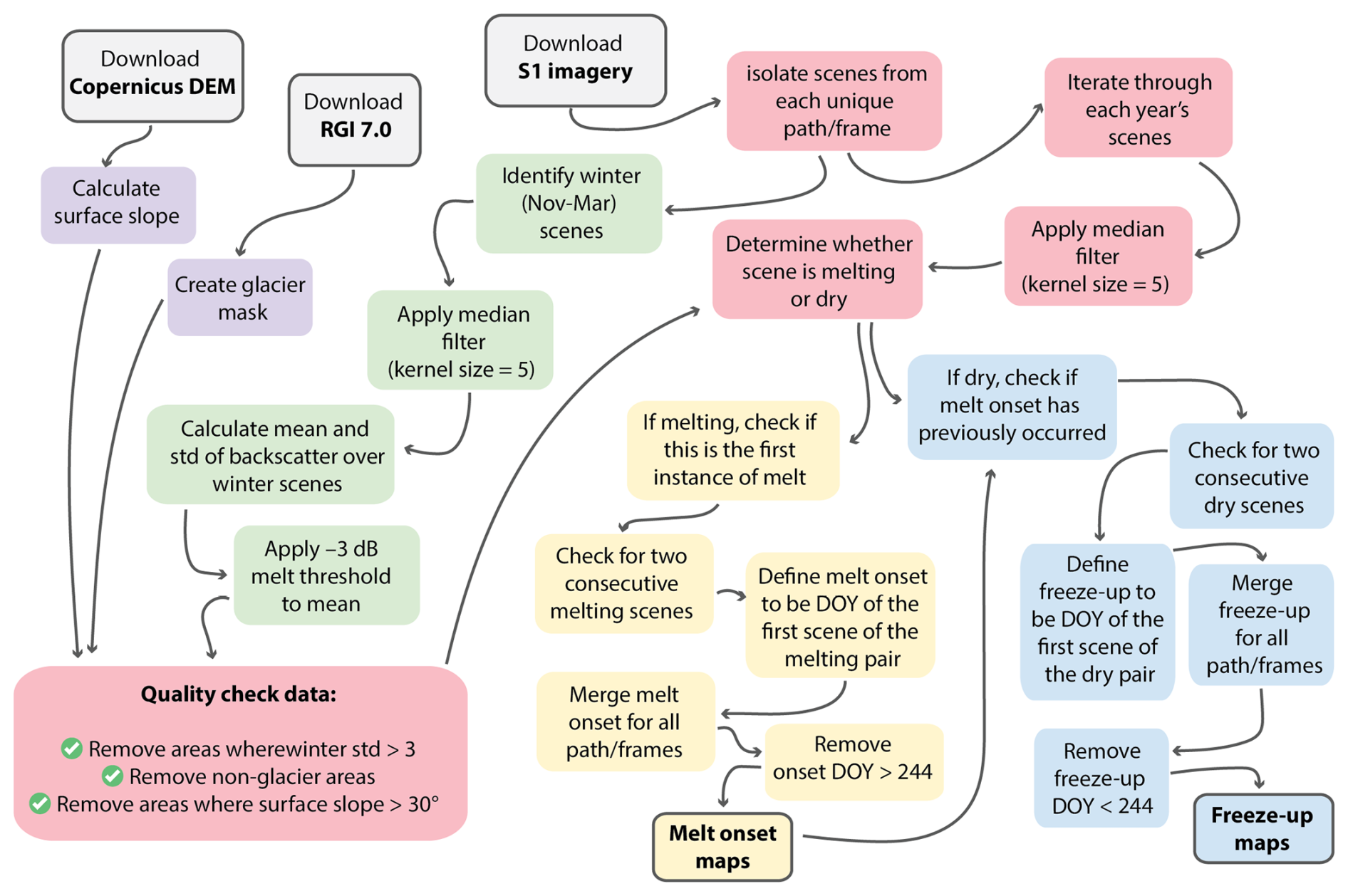
Figure 2 Schematic of processing Sentinel-1 (S1) imagery to derive melt onset and freeze-up day of year (DOY). Gray boxes indicate initial files downloaded. Purple boxes indicate preparatory steps. Green boxes describe the generation of a reference winter dry-snow image. Pink boxes describe the iteration over images in each melt season timeseries, including the execution of a quality check. Yellow boxes describe the determination of melt onset for each pixel. Blue boxes describe the determination of freeze-up for each pixel.

2.4 Image processing

We access and pre-process Sentinel-1 images through the Alaska Satellite Facility (ASF) to produce radiometrically terrain corrected images using ASF’s Hybrid Pluggable Processing Pipeline (HyP3) with the Copernicus DEM at 30 m resolution (Hogenson et al., 2020). During pre-processing, we identify path/frames that intersect our area of interest, and remove those with fewer than four wintertime (November–March) scenes or without scenes after March 31. We then reproject the images and convert backscatter values to decibels (dB; Fig. 2). To reduce speckling in our results, we apply a median filter with a kernel size of 5 to each scene in the dry-snow winter average and in the melt season timeseries, replacing each pixel value with the median of the 5×5 neighborhood centered on that pixel. Pixels where the standard deviation of winter backscatter values is >3 dB (the established melt detection threshold) are excluded from analysis because a 3 dB drop in backscatter is not a deviation from the winter normal range in these areas. We also remove steep (>30°) glacier slopes, which tend to have chaotic and changing ice surfaces that are not conducive to SAR timeseries analysis (Shi and Dozier, 1995), using a mask based on the Randolph Glacier Inventory (RGI) Version 7.0 (RGI 7.0 Consortium, 2023) and the Copernicus DEM (European Space Agency (ESA), 2014), although the methodology is robust to the choice of DEM used to remove steep terrain (Appendix B). The implementation code we build from can be found on Github (Johnson, 2023b).

2.5 Terrain

To investigate the effect of terrain features on melt onset and freeze-up, we implement a Random Forest algorithm with 200 decision trees to quantify the amount of variability in onset and freeze-up that can be explained by elevation, distance from the ocean, slope angle, and aspect (separated into “northness” and “eastness”).

2.6 Air temperatures

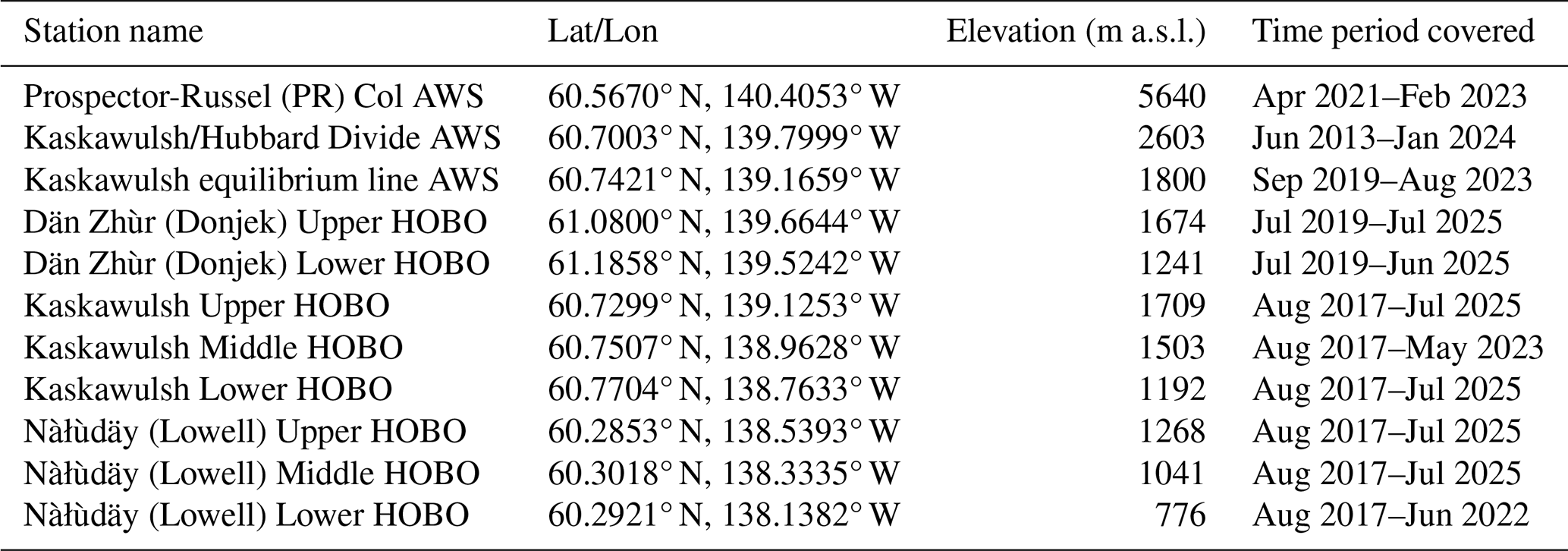
We compare our SAR-based melt detection with air temperature measurements from shielded automatic weather stations (AWS) and HOBO temperature loggers (Table 1) to ground-truth our melt detection and evaluate how well air temperature at the surface represents subsurface firn conditions. To do this, we compare our melt onset and freeze-up results to (1) positive degree days calculated from air temperatures, and (2) the seasonal migration of the 0 °C isotherm. To track the 0 °C isotherm, we first calculate daily regional lapse rates (Fig. C1) from 0 to 5640 m a.s.l. using temperature data from three HOBO sensors (Kaskawulsh Lower, Kaskawulsh Middle, Kaskawulsh Upper) and two AWS (Kaskawulsh/Hubbard Divide and Prospector-Russell Col). We use the Kaskawulsh Upper HOBO data rather than the nearby (within 100 m elevation) Kaskawulsh equilibrium line AWS data because the HOBO sensor is located on glacier ice while the AWS is located on a bedrock nunatak, and the HOBO sensor provides more recent data (Table 1). We select the series of stations going from the lower Kaskawulsh Glacier to Prospector-Russell (PR) Col for its spatial coverage over nearly the entirety of the elevation range within our study domain, and because its temporal coverage began nearly two years earlier than measurements on the nearby Dän Zhùr Glacier (Fig. 1). Note that the PR Col temperature record only covers the time from April 2021 through February 2023; lapse rates outside of this period only utilize data from 0 to 2603 m a.s.l. We perform a least squares linear regression on overlapping mean daily temperature values from all five selected stations (August 2017–February 2023). Finally, we use the resultant daily lapse rates to compute isotherms at 2 °C intervals from −20 to 20 °C for comparison with our melt onset and freeze-up results. A comparison of isotherms computed from Kaskawulsh vs. Dän Zhùr data over their period of overlap (July 2019–February 2023) is provided in Appendix C.

Table 1 Ground-truth air temperature data used in this study. Ground-truth data used in this study. Locations of all stations are shown in Fig. 1. Air temperatures at Prospector-Russel Col were measured using a Vaisala HMP155 temperature sensor inside a solar radiation shield. The sensor experienced no movement over the study period. Sensor accuracy and technical data are available at https://docs.vaisala.com/v/u/B210752EN-K/en-US (last access: 21 October 2025). The Kaskawulsh/Hubbard Divide AWS and Kaskawulsh equilibrium line AWS both used the HOBO S-THB-M002 Temperature/Relative Humidity Sensor (accuracy: ±0.21 °C from 0 to 50 °C; precision: ±0.02 °C from 0 to 50 °C) mounted inside a HOBO RS3 Solar Radiation Shield. Technical data are available at https://www.onsetcomp.com/sites/default/files/resources-documents/11427-O S-THB Manual.pdf (last access: 5 June 2025). Neither of these sensors experienced any movement over the study period. All listed HOBO sensors refer to the HOBO U23-001A Pro v2 Temperature/Relative Humidity Data Logger (accuracy: ±0.25 °C from −40 to 0 °C, ±0.20 °C from 0 to 70 °C; precision: 0.04 °C) mounted inside a HOBO RS1 Solar Radiation Shield. Technical data are available at https://www.onsetcomp.com/products/data-loggers/u23-001a (last access: 5 June 2025). Listed HOBO sensors experienced horizontal (downglacier) movement of approx. 100 m a⁻¹ and vertical movement of approximately −5 to −10 m a⁻¹.

2.7 Hydrologic transition zones

We combine Sentinel-1-derived freeze-up dates, in situ air temperatures, and elevation data to identify regions where delayed firn freeze-up indicates a transition between dry and wet firn regimes. Since our focus here is on firn hydrologic regimes rather than surface melt production, we use the term “dry firn” to refer to firn that does not retain persistent liquid water, even if some surface melting occurs. We identify hydrologic transition zones between dry and wet firn based on the timing of SAR backscatter recovery relative to the annual onset of subfreezing air temperatures (Δfreeze). Where liquid water is retained within the firn, the return to winter backscatter is delayed relative to atmospheric cooling, reflecting progressive refreezing and downward propagation of the freezing front through the firn column (Rau et al., 2000; Winsvold et al., 2018; Scher et al., 2021). Thus, larger Δfreeze values indicate greater persistence of liquid water within the firn.

We analyze Δfreeze values across elevation for individual glaciers within the study domain, as delineated by RGI version 7.0. For each glacier, we calculate the mean Δfreeze value within 50 m elevation bins, excluding glaciers that span less than 1000 m in elevation or are entirely below 2500 m a.s.l. We then calculate the elevation gradient of Δfreeze for each glacier. To reduce short-wavelength variability while preserving broader elevation-dependent patterns, we smooth the resulting gradients using a Savitzky–Golay filter (Savitzky and Golay, 1964) implemented through the savgol_filter function in the Python SciPy package (Virtanen et al., 2020).

We define the hydrologic transition zone as the contiguous region of negative Δfreeze gradients containing the greatest number of elevation bins on each glacier. Negative gradients indicate decreasing Δfreeze with elevation, representing a shift from lower-elevation regions with persistent liquid water retention toward higher-elevation regions characterized by earlier seasonal refreezing. The resulting firn-zone map therefore delineates spatially coherent zones of inferred hydrologic transition based on elevation-dependent variations in seasonal refreeze timing on a per-glacier basis. These zones represent changes in SAR-observed meltwater influence rather than direct observations of firn stratigraphy or classical melt facies.

2.8 Surface energy balance

The energy available for melt can be represented as the net energy balance at the glacier surface (E_N; Cuffey and Paterson, 2010). E_N can be expressed as the sum of component energy fluxes, defined here as positive when they represent a flow of energy into the glacier surface:

$$\begin{array}{}\text{(1)}& E_N=E_{\mathrm{S}}+E_{\mathrm{L}}+E_G+E_{\mathrm{H}}+E_E+E_P\end{array}$$

where E_S is the net shortwave radiation, E_L is the net longwave radiation, E_G is the subsurface energy flux, E_H and E_E are the turbulent sensible and latent heat fluxes, and E_P is the heat flux associated with liquid precipitation that subsequently freezes (Cuffey and Paterson, 2010). A positive E_N will drive melt if the surface has warmed to the melting point, whereas a negative E_N will drive freezing of any available liquid water (Cuffey and Paterson, 2010). Contributions to E_N tend to be dominated by the radiative (E_S and E_L) and turbulent (E_H and E_E) fluxes (Hock, 2005; Cuffey and Paterson, 2010). Because both E_L and E_H increase with atmospheric temperature, atmospheric warming is a key driver of surface melt production; however, the magnitude of its effect on E_N varies over space and time (Cuffey and Paterson, 2010).

To compare the relative contributions of radiative and turbulent fluxes to the surface energy balance across elevations, we apply the surface energy balance model of Matthews et al. (2020), previously developed for a similar glacierized alpine environment in the Himalaya, to AWS data from three sites: PR Col (5640 m a.s.l.), the Kaskawulsh/Hubbard Divide (2603 m a.s.l.), and the Kaskawulsh equilibrium line (1800 m a.s.l.; Fig. 1; Table 1). Our surface energy balance modeling is not intended to predict or reproduce observed melt rates, but rather to evaluate the physical plausibility of melt occurring during periods of below-freezing air temperatures. The model is used as a first-order physical constraint: if available energy is sufficient to produce melt despite sub-zero air temperatures, this supports the interpretation that air temperature alone is insufficient to determine melt occurrence in high-elevation glacier environments. Therefore, simplified parameterizations are used to estimate whether the net surface energy balance can become positive under observed meteorological conditions. This approach is appropriate for identifying whether melt is energetically possible, while recognizing that uncertainties in albedo, cloud radiative effects, and atmospheric emissivity introduce uncertainty into the magnitude of calculated melt energy.

Incoming shortwave radiation is measured directly at all three AWS sites and combined with a prescribed constant albedo of 0.8 (old, clean, dry snow; Cuffey and Paterson, 2010), applied uniformly across sites and time, to calculate E_S. Although snow surface albedo can vary widely (0.5–0.98; Cuffey and Paterson, 2010), higher elevations are generally characterized by dry, minimally metamorphosed snow and thus higher albedo. As a result, our estimates of the relative contribution of shortwave radiation to surface energy balance at PR Col compared to the lower sites are likely conservative. The effects of cloud-enhanced shortwave radiation through multiple scattering were not explicitly represented. This process may increase incoming shortwave radiation under partial cloud cover; however, resolving these effects would require a more sophisticated radiative transfer scheme beyond the scope of this diagnostic analysis.

Net longwave radiation is estimated using the Brutsaert (1975) clear-sky emissivity parameterization based on measured air temperature and relative humidity. The Brutsaert (1975) formulation estimates clear-sky emissivity from near-surface atmospheric variables and does not explicitly represent cloud contributions to atmospheric emissivity. Consequently, longwave radiation estimates may be biased low under cloudy conditions, where atmospheric emissivity is enhanced. Because the analysis focuses on identifying conditions favorable for melt rather than estimating melt volumes, we interpret modeled melt energy as a first-order estimate of available energy. Turbulent heat fluxes are calculated using the bulk aerodynamic method (Hock, 2005), with identical parameterizations applied at all sites. We run the model with 2 min timesteps to resolve diurnal variability and then downsample output fluxes to daily means.

3 Results

3.1 Surface melt onset

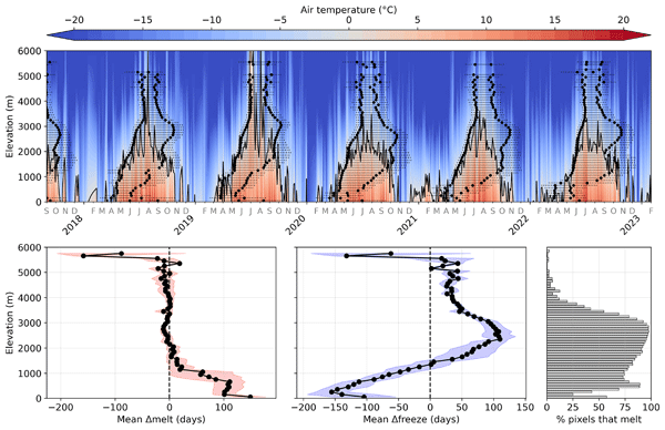
We detect seasonal melting across virtually all elevations (up to 5908 m a.s.l.) in the Wrangell/St. Elias Mountains. However, the percentage of pixels that experience melt drops from >85 % between 2000 and 3000 m a.s.l. to <15 % between 4000 and 5000 m a.s.l. to only 1 % of pixels above 5000 m a.s.l. (Fig. 4d).

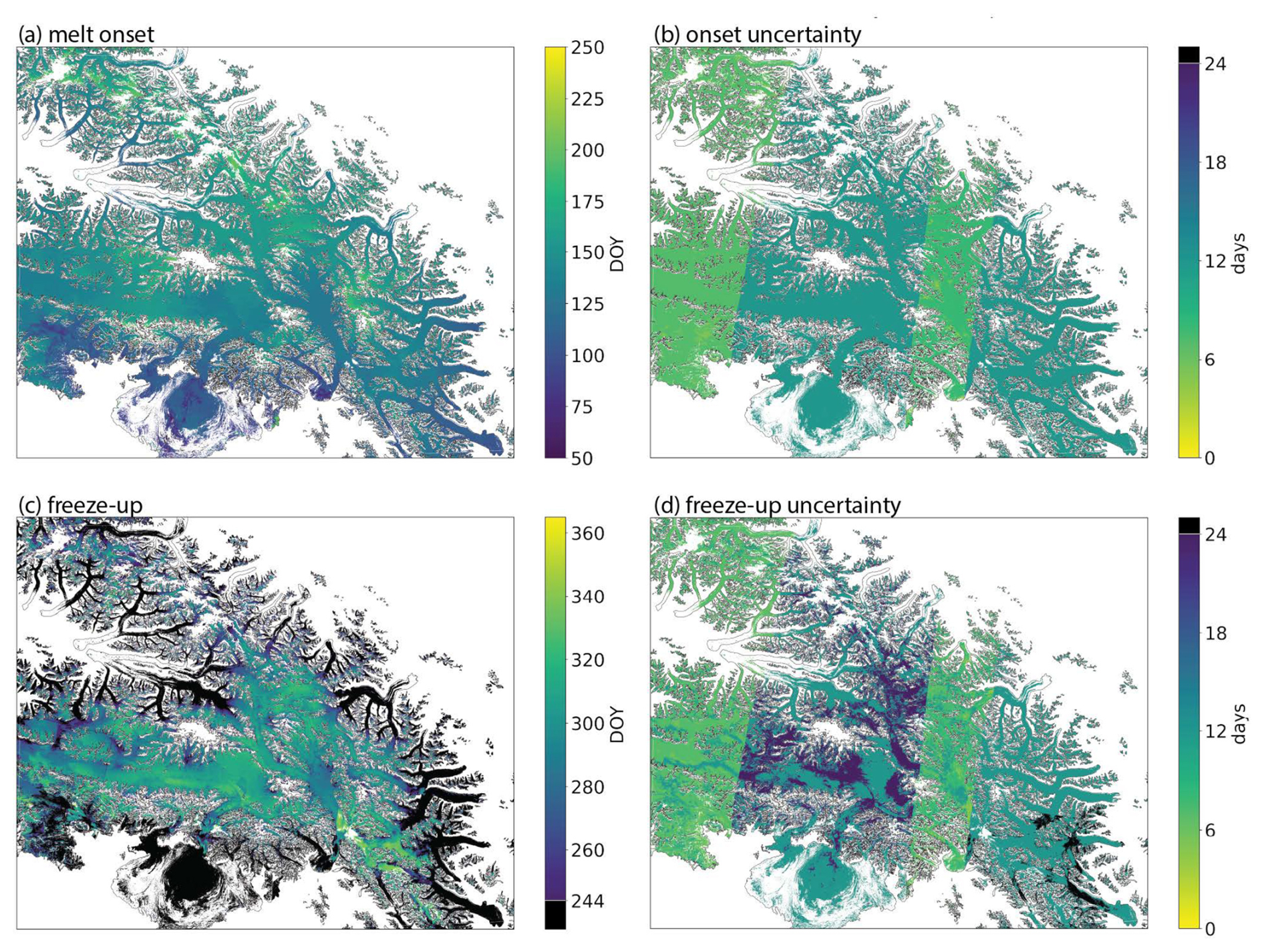
Figure 3 Spatial distribution of mean melt onset (a) and freeze-up (c) day of year (DOY) from 2018–2021, and the associated uncertainty in days (b, d).

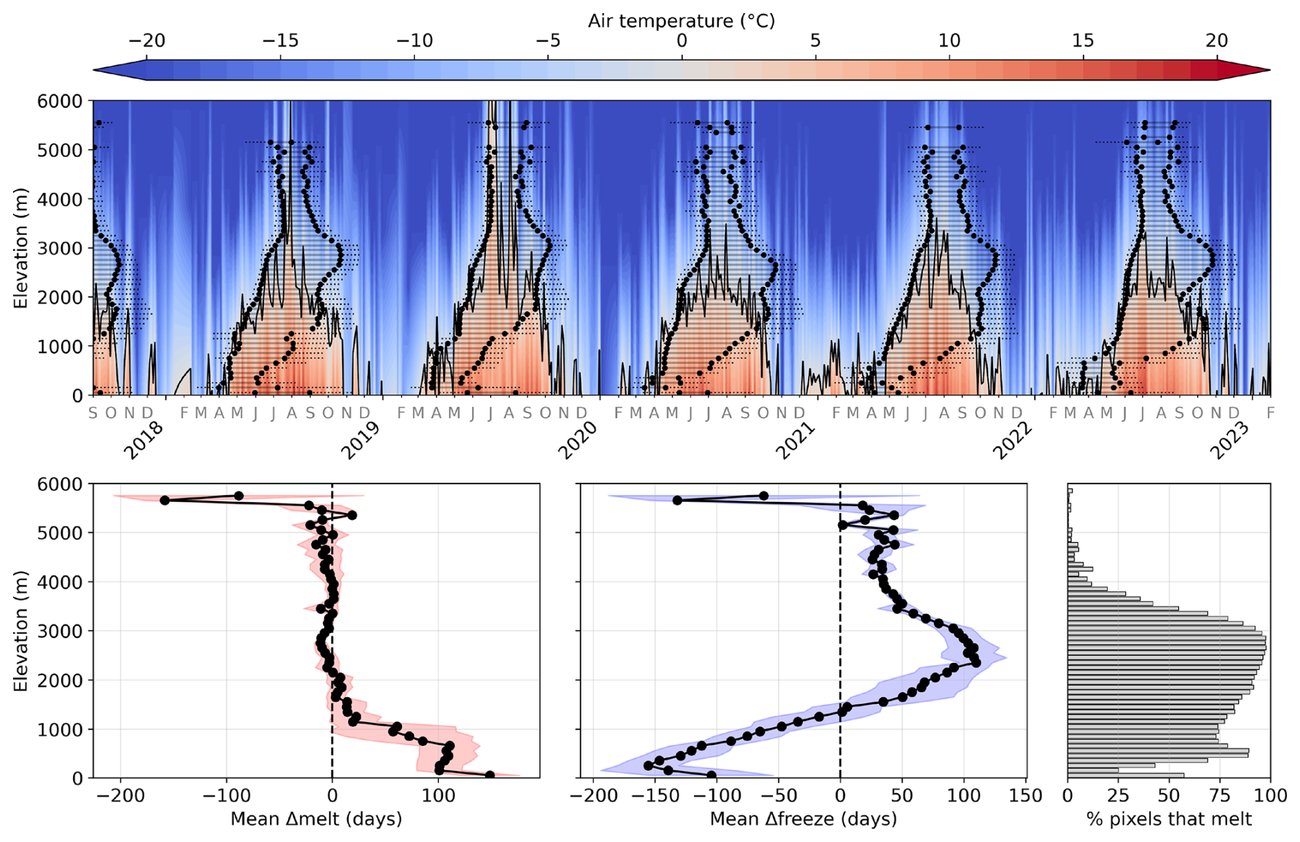
Figure 4 Mean melt onset and freeze-up relative to seasonal migration of the 0 °C isotherm. Panel (a) shows melt onset and freeze-up dates (black solid circles) averaged over 100 m elevation bins plotted with spatially integrated air temperatures (colorbar). Air temperatures were estimated from lapse rates computed using data from five in situ stations ranging in elevation from 1192–5640 m a.s.l. The black line represents the 0 °C isotherm. Panel (b) shows the offset between Sentinel-1 melt onset and the DOY of 0 °C air temperatures across elevation bands (Δmelt). Panel (c) shows the offset between Sentinel-1 freeze-up and the DOY of 0 °C air temperatures across elevation bands (Δfreeze). Δmelt is averaged across 2018–2022. Δfreeze is averaged across 2017–2022. Standard deviations are shown by the shaded red (melt) and blue (freeze) envelopes. Panel (d) shows the percentage of pixels in each elevation band that melt.

From 2018–2021 (years with >45 % Sentinel-1 coverage over the glacierized portion of our study domain), we find melt onset across much of Wrangell/St. Elias to occur on average between day of year (DOY) 125 and 175 (approximately 5 May to 25 June, Fig. 3). Melt onset and freeze-up maps for individual years 2015–2024 can be found in Appendix E. A comparison of melt onset with positive degree days calculated from in situ measurements can be found in Appendix F.

Melt onset occurs later as elevation increases, closely tracking the upward migration of the 0 °C isotherm until around 3000 m a.s.l., providing validation for SAR-based melt detection. Note, however, that the most consistent onset dates and strongest coherence with above-freezing air temperatures occur below 3000 m a.s.l. (Fig. 4). Above 3000 m a.s.l., the 0 °C isotherm no longer rises systematically, and melt onset occurs at similar DOY even as elevation increases (Fig. 4a). Although elevation is the dominant determinant of melt onset across our study domain, there is a reduction in its importance relative to other terrain characteristics above 3000 m a.s.l. (Fig. 5). When considered together across the entire study domain, elevation, distance from ocean, slope angle, and aspect explain 61 % of variability in melt onset date, with an average prediction error of 12 d (random forest analysis).

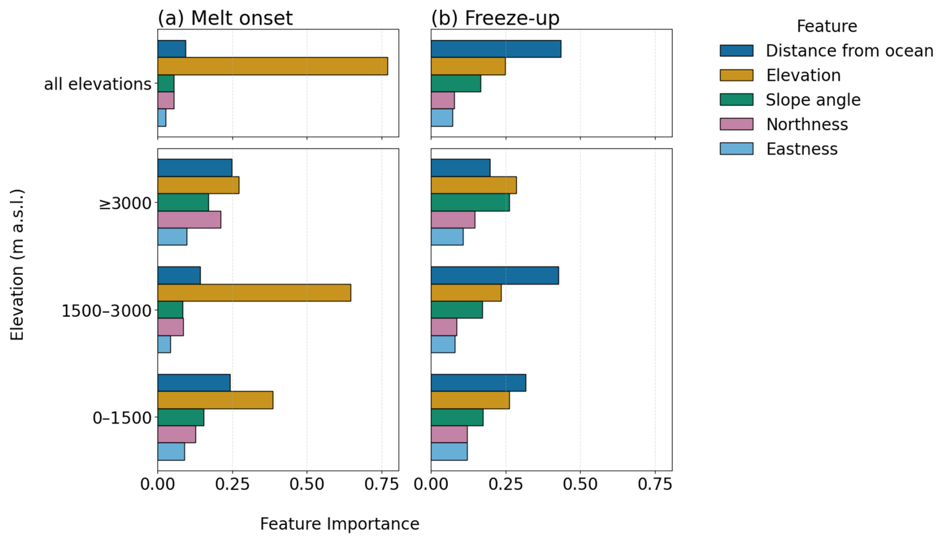
Figure 5 Relative importance of terrain features in determining melt onset (a) and freeze-up (b) dates. Relative importance over all elevations is shown in the top set of panels. Relative importance for pixels at low (0–1500 m a.s.l.), middle (1500–3000 m a.s.l.) and high (above 3000 m a.s.l.) elevations are shown in the bottom set of panels.

3.2 Firn freeze-up

Freeze-up across much of Wrangell/St. Elias from 2018–2021 occurs on average between DOY 260 and 340 (approximately 17 September to 6 December, Fig. 3).

Freeze-up does not mirror the downward migration of the 0 °C isotherm in the fall (Fig. 4). Below 1400 m a.s.l., Δfreeze < 0 d, meaning winter firn conditions are reached as the snowline migrates to higher elevations before air temperatures drop below 0 °C. Δfreeze increases with elevation until 2400 m a.s.l. Freeze-up is most delayed relative to 0 °C air temperatures between approximately 2400 and 2900 m a.s.l. (Δfreeze > 100 d). Δfreeze decreases with elevation from 2900 m a.s.l. to 3500 m a.s.l. Between 3500 and 5000 m a.s.l., 25 < Δfreeze < 50 d.

When considered together across all elevations, five terrain characteristics (Fig. 5) explain 25 % of variability in freeze-up date, with an average prediction error of 24 d. Distance from ocean shows the greatest predictive capacity for freeze-up (negatively related) below 3000 m a.s.l., while its importance is reduced relative to elevation and slope angle above 3000 m a.s.l. (Fig. 5).

3.3 Hydrologic transition zones

Based on the behavior of firn freeze-up across our study domain (Fig. D1), we find that 3 % (702 km²) of the glacierized area in our study domain is in a dry firn zone, and 9 % (2142 km²) is in a hydrologic transition zone (Fig. 6). We find hydrologic transition zones to be concentrated on the continental side of the range and/or on the flanks of high peaks, with hydrologic transition zones on the continental side tending to be higher in elevation than those closer to the coast (Fig. 7).

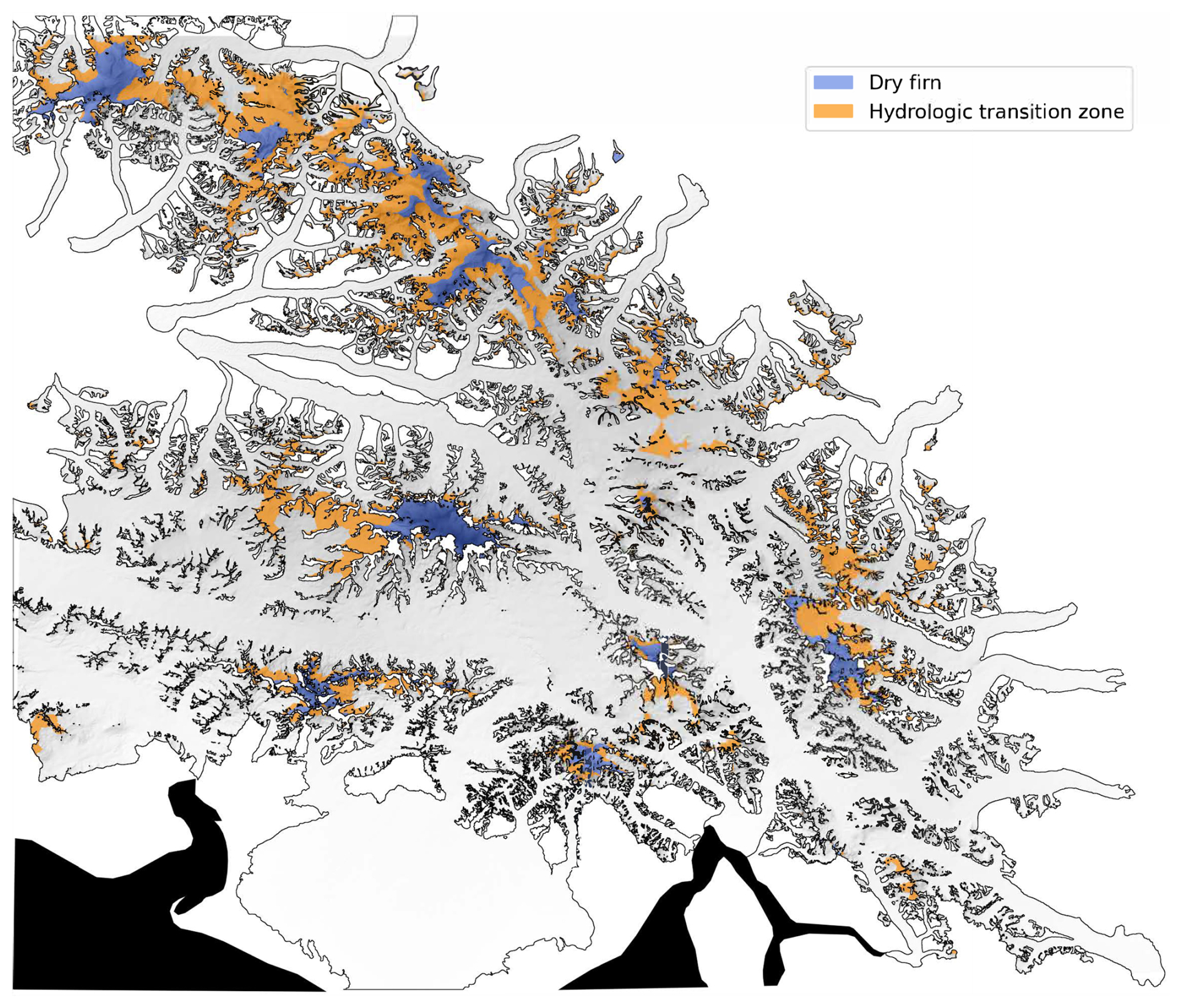
Figure 6 Hydrologic transition zones across the study area from 2018–2022 derived from Sentinel-1 freeze-up timing, air temperature, and elevation. Glacierized area are shown in hillshade overlain with dry firn (blue) and hydrologic transition zones (orange). The Gulf of Alaska is shown in black.

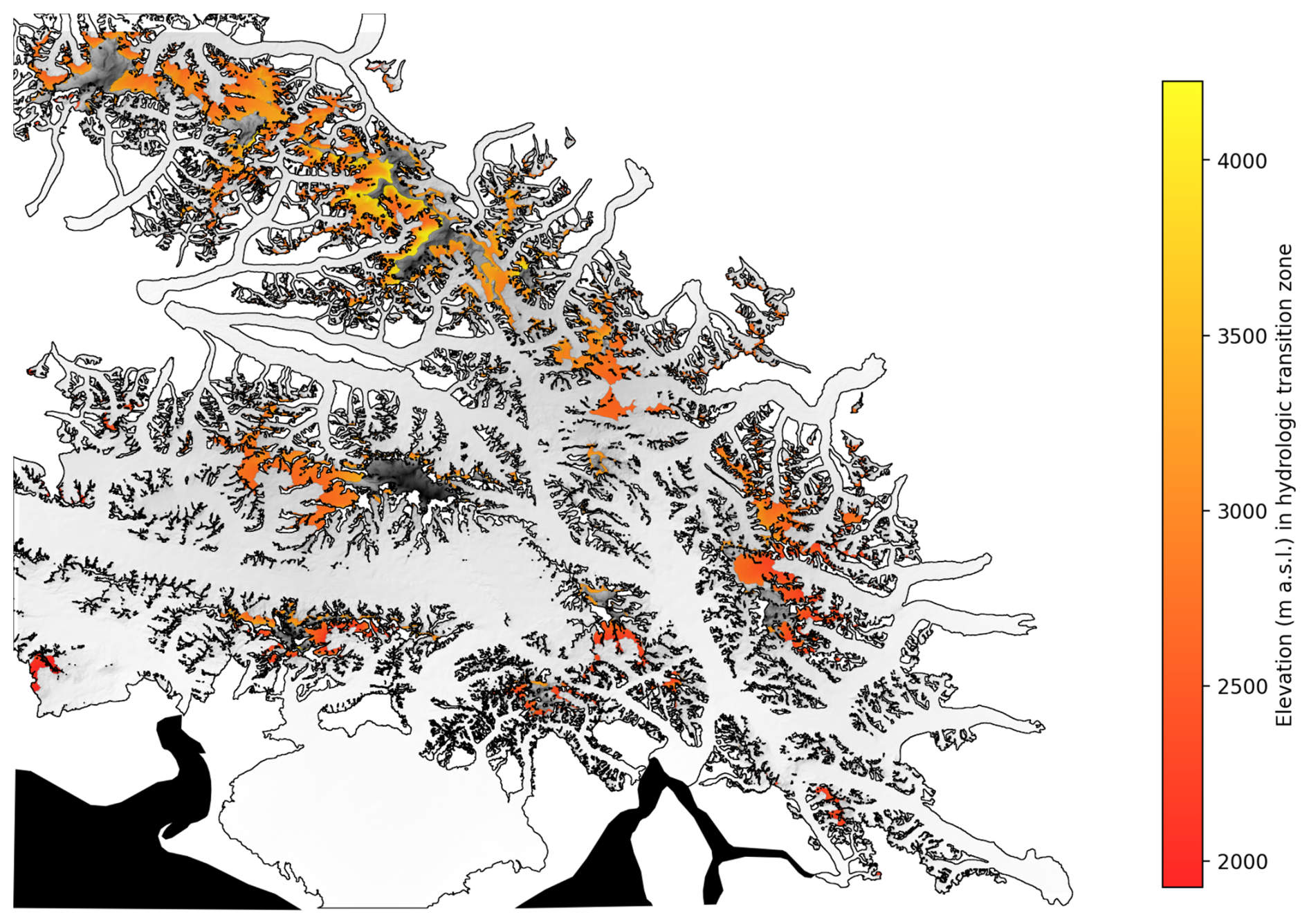
Figure 7 Elevation of hydrologic transition zones across the study area from 2018–2022 derived from Sentinel-1 freeze-up timing, air temperature, and elevation. Glacierized area are shown in hillshade overlain with hydrologic transition zones colored by elevation. The Gulf of Alaska is shown in black.

3.4 Surface energy balance

Radiative heat fluxes are predominantly positive at the Kaskawulsh/Hubbard Divide and the Kaskawulsh equilibrium line, while turbulent fluxes are predominantly negative, aside from a summer interval of positive sensible heat flux. At PR Col, only net shortwave radiation is predominantly positive (Fig. 8).

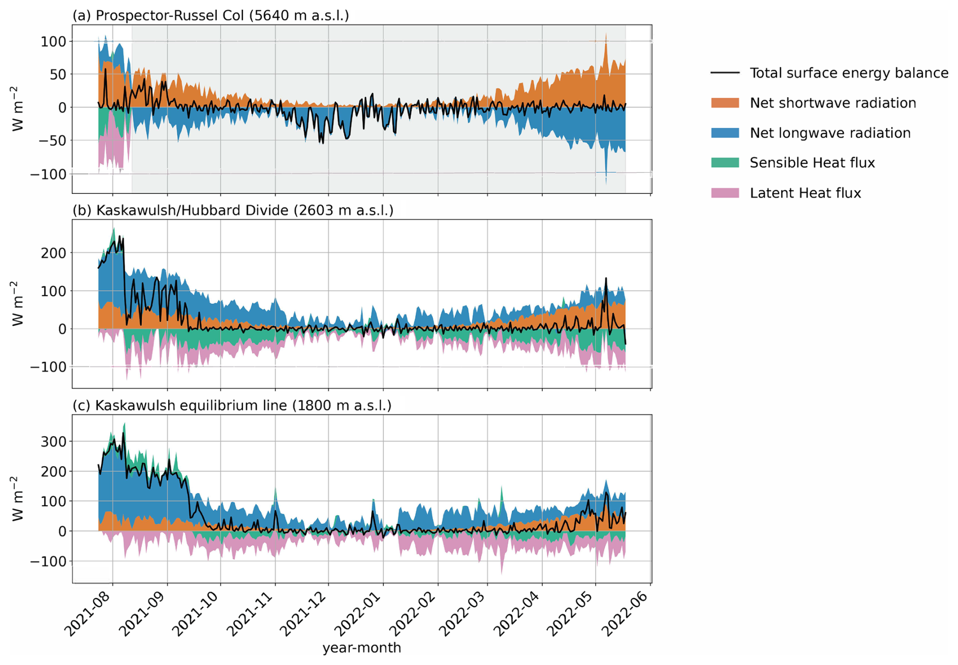
Figure 8 Modeled components of the surface energy balance (surface energy balance) at Prospector-Russel Col (a), the Kaskawulsh/Hubbard Divide (b), and the Kaskawulsh equilibrium line (c). The net surface energy balance is shown by a black line, while individual components are shown in the stacked line plot. The gray shaded area in panel (a) indicates the period of time when wind speed measurements used to calculate the sensible and latent heat fluxes were unavailable at PR Col. Because the analysis focuses on relative flux contributions using identical model parameterizations across sites, systematic uncertainties are expected to affect all sites similarly and are therefore not shown.

4 Discussion

4.1 Surface melting and energy balance

The relatively constant range of melt onset dates in Wrangell/St. Elias across elevations >3000 m a.s.l. compared to at lower elevations may reflect the outsized influence of incoming solar radiation relative to air temperatures in producing melt above >3000 m a.s.l. Generally, longwave radiation is a dominant component in surface energy balance and contributor to surface melting (Cuffey and Paterson, 2010), which is reflected in the correspondence between surface melt onset and the migration of the 0 °C isotherm (Fig. 4). However, surface melting can be driven by shortwave radiation (insolation) even when air temperatures remain below 0 °C, as they largely do at higher elevations in our study domain (Matthews et al., 2020; Scher et al., 2021). Notably, we detect surface melting in a small (<15 %) but non-zero percentage of pixels above 4000 m a.s.l. despite a near absence of above-freezing air temperatures.

Our surface energy balance modeling indicates that net shortwave radiation is the positive dominant contribution to surface energy balance at PR Col, compared to the Kaskawulsh/Hubbard Divide and Kaskawulsh equilibrium line, where longwave radiation dominates. At the lower two sites, the sensible heat flux also represents a small positive contribution during summer. In contrast, both the sensible and latent heat fluxes are negative when calculated at PR Col. Wind speeds for turbulent flux heat calculations at PR Col were only available 24 July to 11 August 2021 (Fig. 8). However, July and August are during the height of the melt season, when we would expect turbulent fluxes to be the least negative (or most positive). We therefore expect the turbulent heat fluxes at PR Col to be predominately negative year-round.

4.2 Hydrologic transition zones

Below 1400 m a.s.l., Δfreeze < 0 d, meaning winter firn conditions are reached before air temperatures drop below 0 °C. In this case, winter conditions refer to dry snow underlain by bare ice rather than by dry firn. These negative Δfreeze values therefore reflect the melting of snow down to bare ice, rather than refreezing of wet firn. Because our focus is on firn hydrology, the following discussion centers around hydrologic transition zones between dry and wet firn, rather than low-elevation areas with late-summer bare ice.

We find only 12 % of the glacierized area in our study domain to comprise dry firn (3 %) and hydrologic transition zones (9 %). Our results indicate that liquid water plays a central role in shaping near-surface physical properties across the majority of Wrangell/St. Elias, and underscore the importance of continuing to develop robust and spatially distributed meltwater percolation models for use in alpine environments. The limited extent of dry firn has direct implications for the preservation of ice core paleoclimate archives, as meltwater percolation and refreezing in wet firn can disrupt stratigraphy and preclude ice core drilling. As a result, opportunities to recover regional ice core records in Wrangell/St. Elias are already limited (Holland et al., 2026), and are likely to diminish with ongoing atmospheric warming.

We find hydrologic transition zones to occur anywhere from 1925 to 4225 m a.s.l., with the 10–90 percentile range being from 2467–3393 m a.s.l. (Fig. 7). The lower bounds of our hydrologic transition zones are characterized by high Δfreeze values that indicate the persistence of liquid water within the firn into the fall, consistent with in situ observations of a firn aquifer near the Kaskawulsh/Hubbard Divide at approximately 2640 m a.s.l. (Ochwat et al., 2021). Note that a delay in summer-to-winter backscatter rebound (high Δfreeze) does not necessarily imply a firn aquifer; a similar backscatter response can be expected from percolation and delayed refreeze even if an aquifer never forms.

We define our hydrological transition zones as spatial transitions between higher areas of dry firn and lower areas of wet firn. However, we interpret these spatial transition zones as also reflecting a temporal transition: sites within these zones appear to be in the process of evolving from dry to increasingly wet firn states (e.g. increased percolation and delayed refreeze). This interpretation is supported by in situ observations and firn pack modeling at Eclipse Icefield (Fig. 1) which suggest the site is undergoing a temporal transition from a mostly dry firn pack to one that can and does support persistent liquid water into the fall and winter (Kindstedt et al., 2025). If wetting of the firn continues to the point of saturation, this transition could support the eventual development of a firn aquifer. Even barring aquifer development, continued firn wetting will alter firn column structure and the timing of seasonal discharge from firn at these elevations.

The method applied here is able to identify zones of hydrological transition; however, it does not provide information on other aspects of melt production and storage, such as melt season intensity, total melt production, or the partitioning of meltwater between storage in the snow/firn column and runoff. Such factors are necessary to quantify the contribution of surface melt to glacier mass balance and assess downstream hydrological impacts. Notably, the variability in Δfreeze between 3000–3400 m a.s.l. suggests variation in melt season intensity, total melt production, and/or meltwater transport without a corresponding shift in melt onset, underscoring that onset alone is not a sufficient descriptor of seasonal melt dynamics. Nevertheless, in a region defined by pronounced seasonality, melt onset remains a valuable metric that establishes temporal context for subsequent melt, percolation, and refreezing processes. Future work should focus on the quantity and duration of meltwater retention in the firn, thereby enabling a more complete assessment of meltwater generation and its implications for both local glacier evolution and regional hydrology.

5 Conclusions

In this study, we present a spatially distributed assessment of seasonal surface melt onset and firn freeze-up across the Wrangell/St. Elias Mountains using satellite radar backscatter. By deriving melt timing metrics that are independent of air temperature, we provide a region-wide characterization of surface melting and refreezing processes beyond the limits of in situ observations and temperature-based melt estimates. In particular, we show that surface melting can occur even where air temperatures remain below freezing year-round. Our results demonstrate the value of satellite SAR imagery for monitoring melt dynamics in complex, data-sparse mountain regions, while also highlighting the spatial variability of melt onset and the importance of local context when interpreting SAR signals.

We show that seasonal melt is widespread across the region, with dry firn accounting for only 3 % of the study area, substantially limiting the extent of firn capable of preserving undisturbed paleoclimate records. Seasonal backscatter evolution further indicates that meltwater persistence and delayed refreezing are common at mid-elevations, consistent with in situ observations and firn modeling that suggest increasingly water-rich firn conditions. Together, these findings highlight the central role of meltwater percolation and refreezing in shaping firn structure across much of Wrangell/St. Elias.

While the approach presented here is limited to resolving the timing of melt onset and freeze-up, and subsequently deriving hydrological transition zones, these results provide a baseline for evaluating ongoing changes in glacier surface melt, alpine firn evolution, and downstream hydrological impacts in the Wrangell/St. Elias Mountains.

Appendix A: Sentinel-1 scenes used in this study

Table A1 Sentinel-1 scenes used in this study. Total path/frames and Total scenes are the total numbers of unique path/frames and scenes, respectively, over our area of interest each year. Path/frames used and Scenes used are the numbers of path/frames and scenes, respectively, used in our analysis after filtering. All scenes were obtained in the interferometric wide (IW) beam mode and in co-polarization.

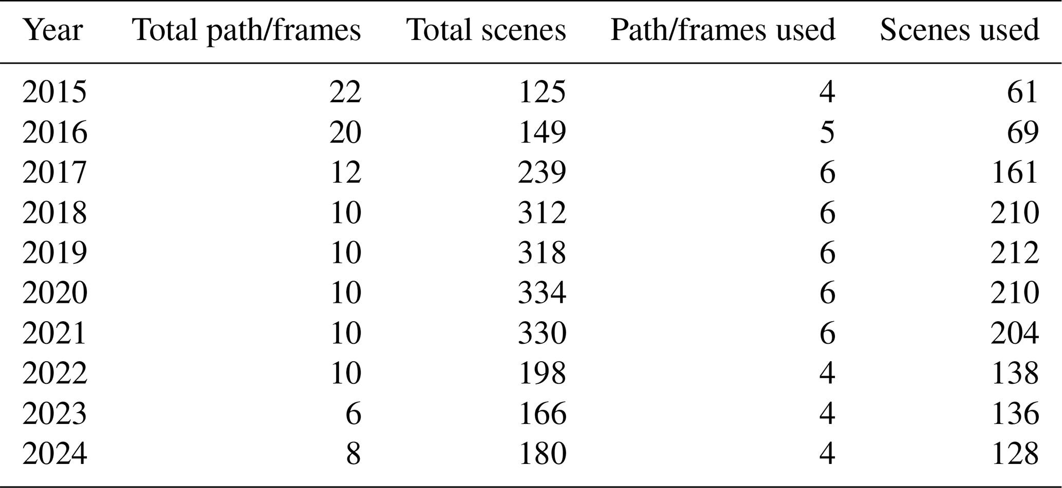
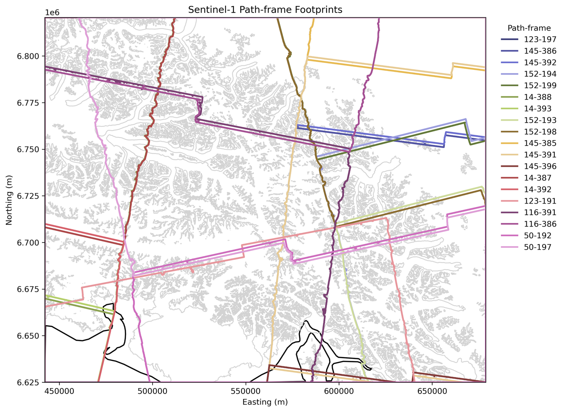
Figure A1 Footprints of all the Sentinel-1 path-frames intersecting our study domain. Glacier outlines are shown in light gray. The Gulf of Alaska coast is shown in black.

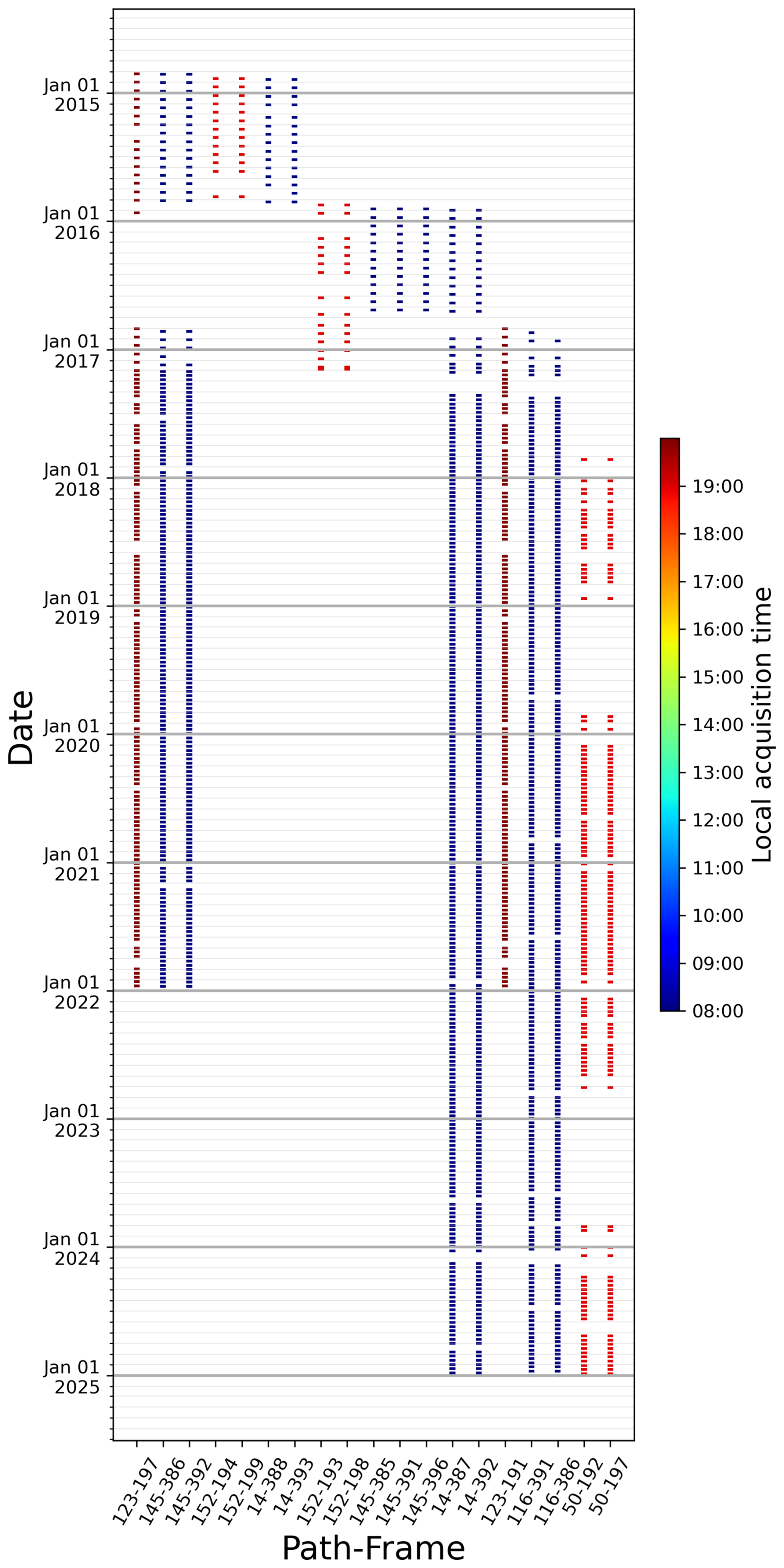
Figure A2 Dates and times of Sentinel-1 image acquisition for path-frames intersecting our study domain.

Appendix B: Evaluation of DEM choice in deriving surface slope

To evaluate the impact that our choice of DEM has on the 30° slope threshold used in this analysis, we compared slopes derived from the 30 m Copernicus DEM with slopes derived from the 10 m ArcticDEM resampled to the same 30 m grid. The comparison was restricted to glacierized pixels where both DEMs contain valid data. Differences between slope fields showed no systematic bias (median difference = 0.0°; mean difference = 1.25°). Although localized differences occurred in areas of complex topography (RMSE = 7.07°; standard deviation = 6.96°), the two DEMs produced similar total areas of steep terrain. Areas classified as >30° slopes represented 21.5 % of glacierized terrain using the Copernicus DEM (9702 km²) and 23.8 % using ArcticDEM (10 724 km²). Differences between the two classifications were limited to 6.2 % of glacierized pixels, with ArcticDEM identifying a greater extent of steep terrain (+1022 km²) relative to Copernicus.

Appendix C: Isotherm computation from in situ temperature data

Figure C1 Lapse rates computed from Kaskawulsh and Dän Zhùr air temperature data over their period of overlap (July 2019–February 2023). In situ data were used to calculate lapse rates. Station locations shown in Fig. 1, and station information in Table 1.

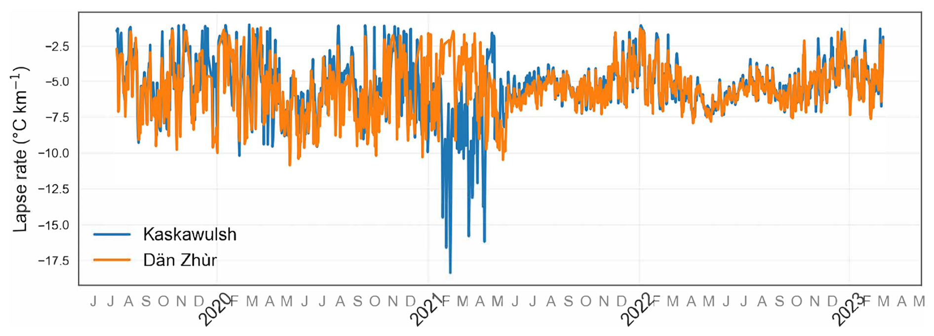
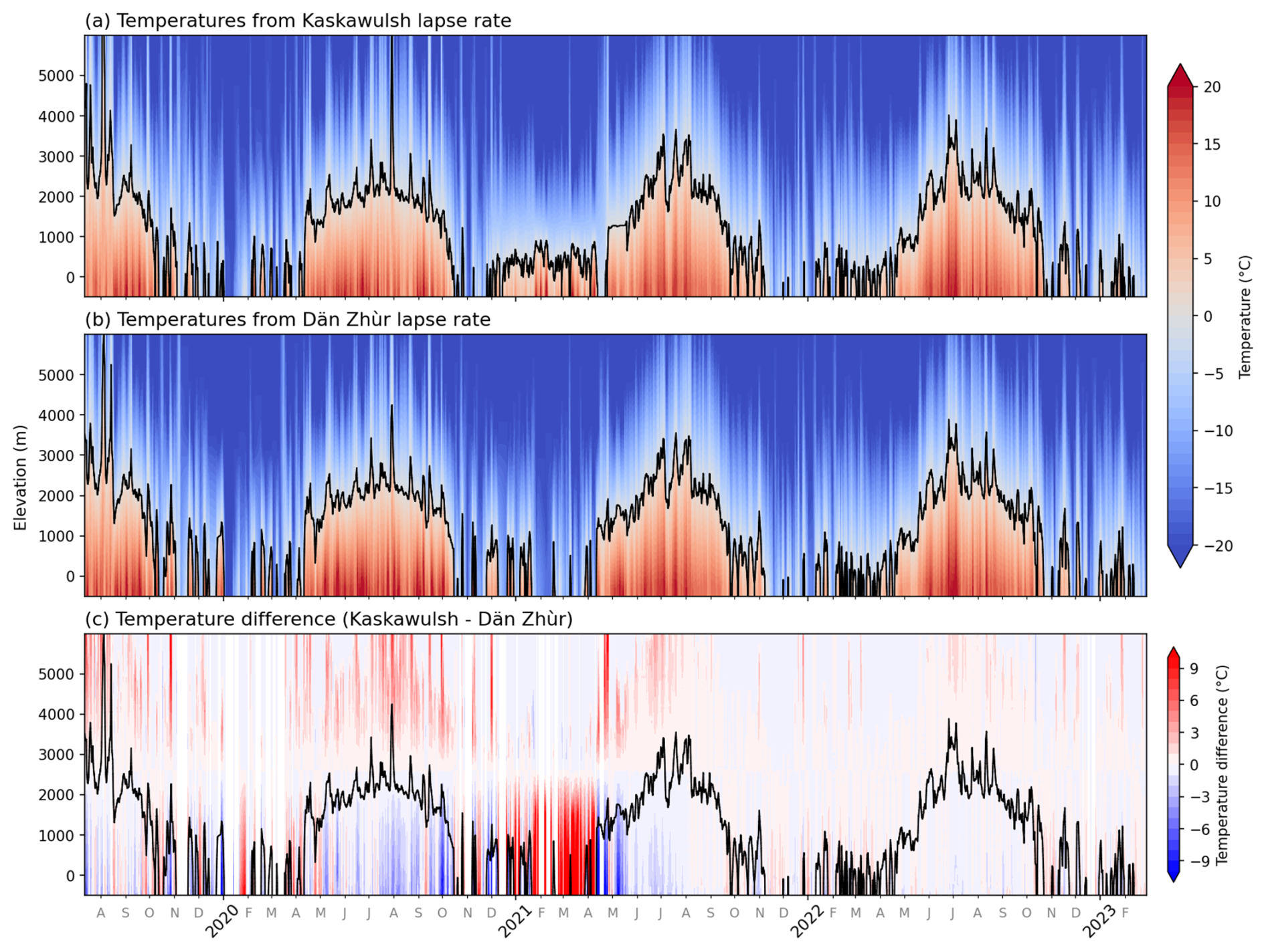
Figure C2 Isotherms computed from Kaskawulsh vs. Dän Zhùr air temperature data over their period of overlap (July 2019–February 2023). In situ data were used to calculate lapse rates, which were in turn used to estimate temperatures by elevation. Panel (a) shows temperature estimates based on in situ measurements from the Kaskawulsh Glacier. Panel (b) shows temperature measurements based on in situ data from the Dän Zhùr Glacier. Panel (c) shows the difference between the two. Station locations shown in Fig. 1, and station information in Table 1.

Appendix D: Definition of firn zones

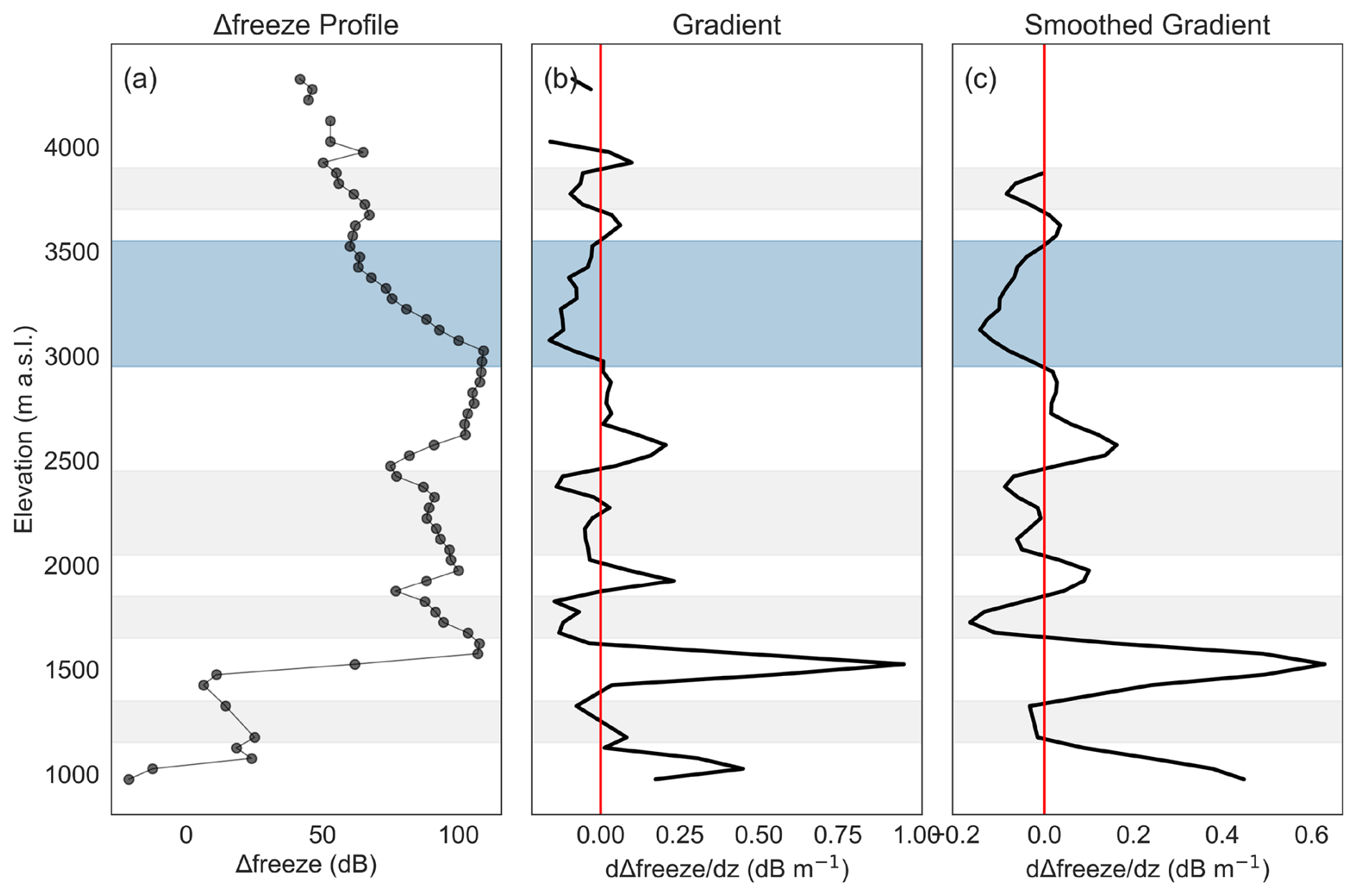
Figure D1 Δfreeze profile (a), vertical gradient (b), and smoothed vertical gradient (c) used to define hydrological transition zone on the Dan Zhur (Donjek) Glacier. Smoothing is done using a Savitzky–Golay filter. The vertical gray lines in panel (b) and (c) indicate a vertical Δfreeze gradient of zero. Horizontal shaded gray bars show all zones of negative Δfreeze gradients. The horizontal shaded blue bar shows the hydrologic transition zone.

Appendix E: Melt onset and freeze-up maps for individual years

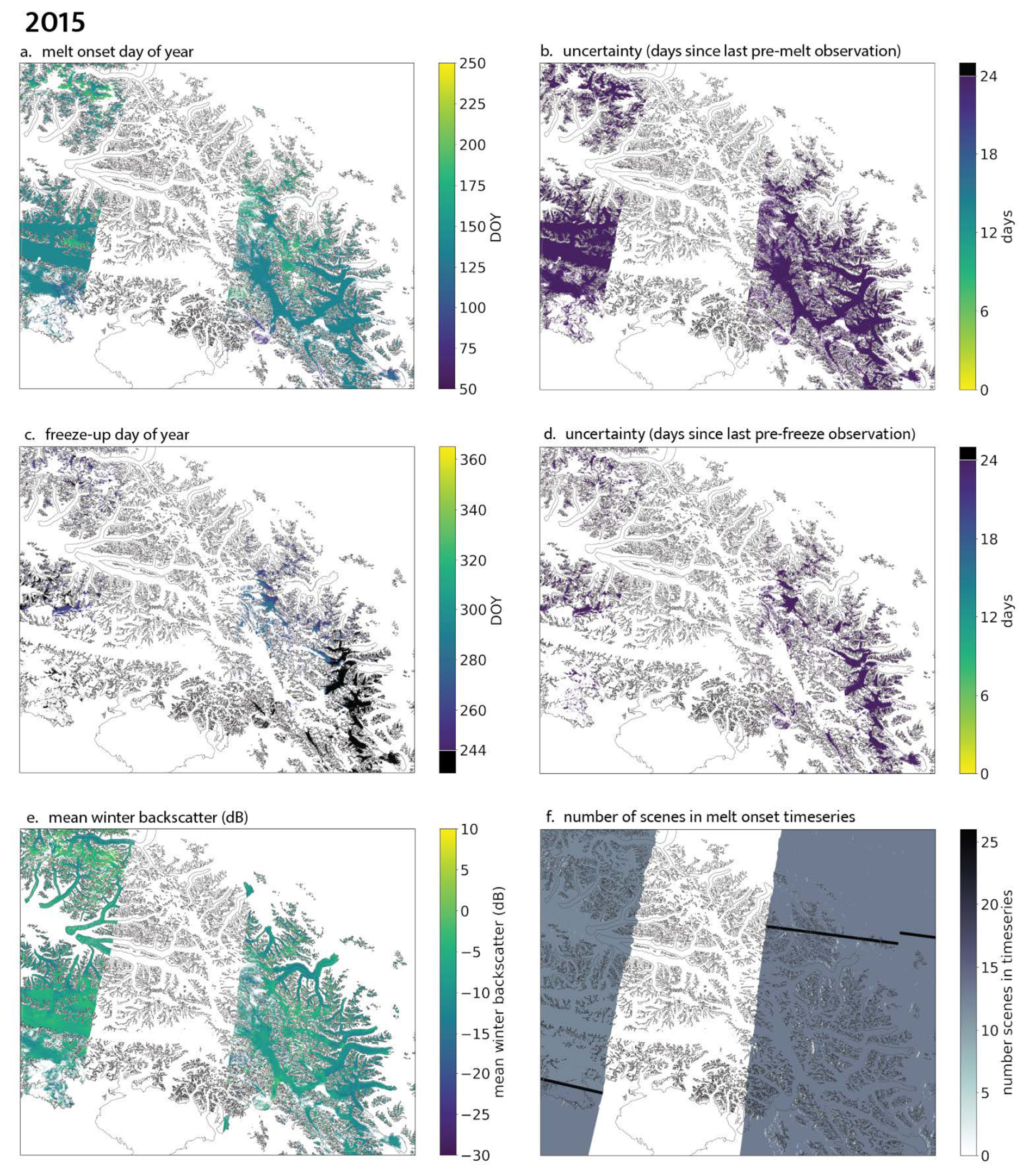
Figure E1 Melt onset (a), onset uncertainty (b), freeze-up (c), freeze-up uncertainty (d), mean winter backscatter (e), and number of scenes (f) over our study domain for 2015.

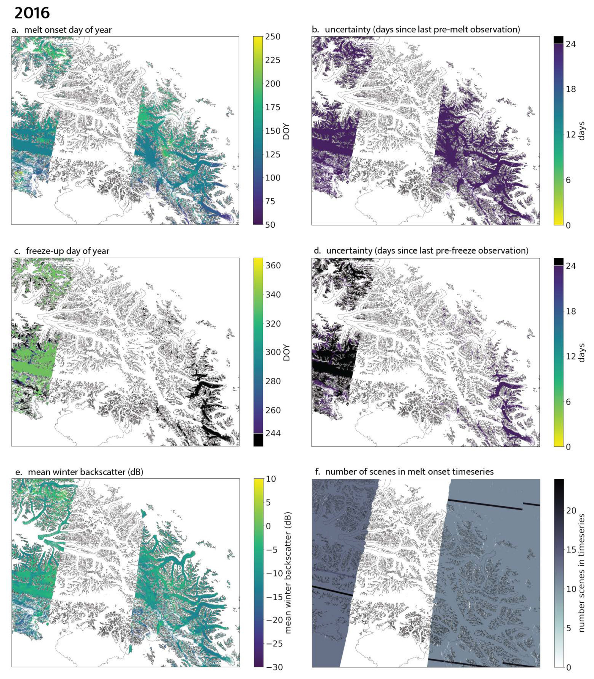
Figure E2 Melt onset (a), onset uncertainty (b), freeze-up (c), freeze-up uncertainty (d), mean winter backscatter (e), and number of scenes (f) over our study domain for 2016.

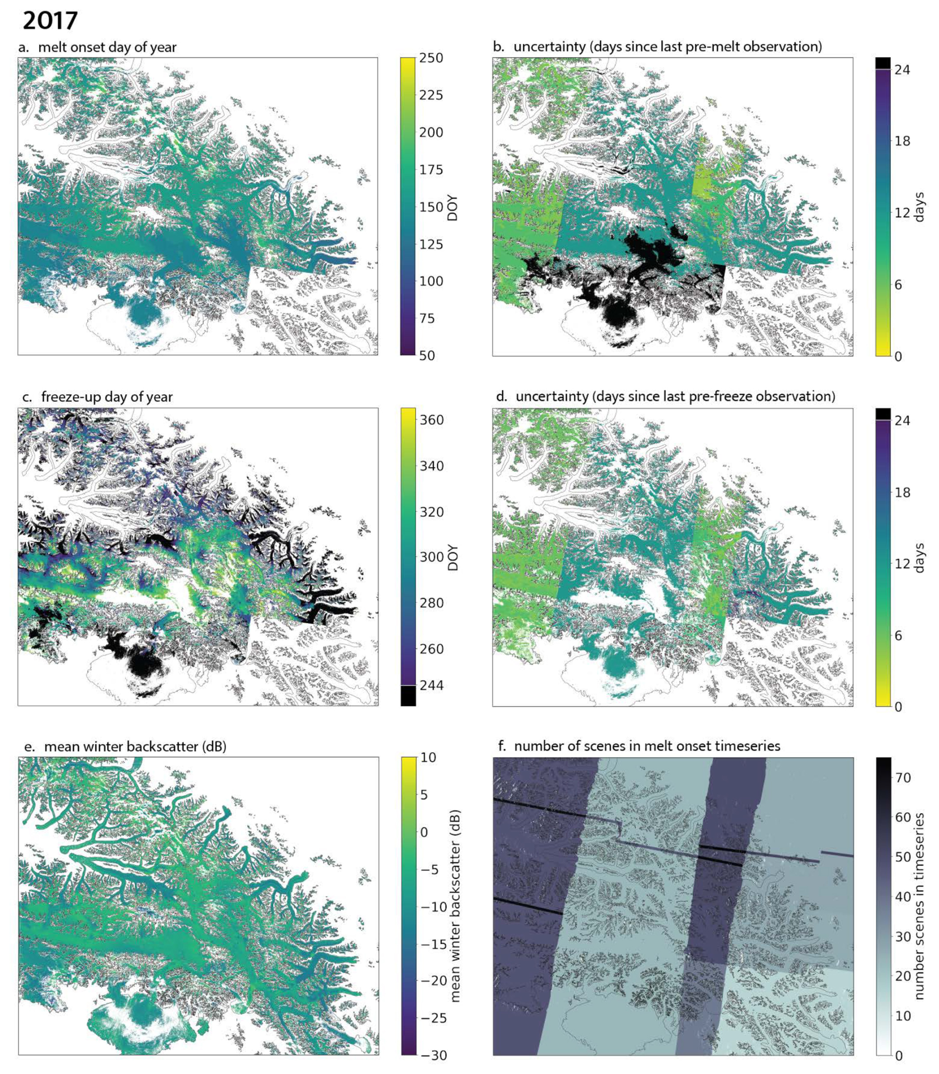
Figure E3 Melt onset (a), onset uncertainty (b), freeze-up (c), freeze-up uncertainty (d), mean winter backscatter (e), and number of scenes (f) over our study domain for 2017.

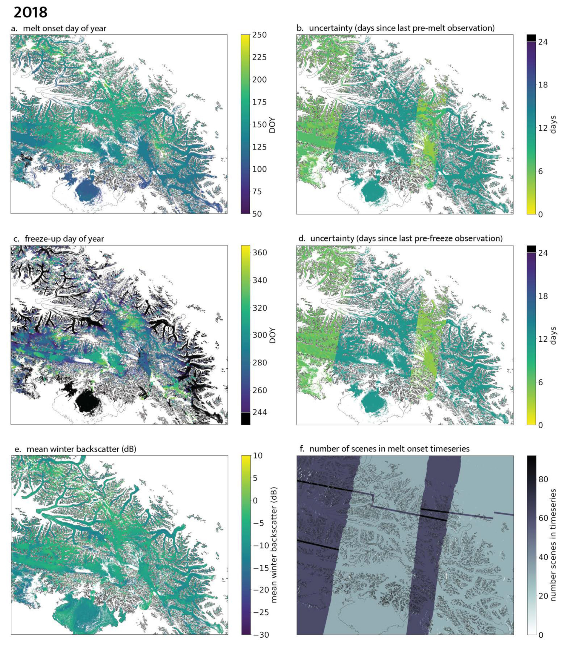
Figure E4 Melt onset (a), onset uncertainty (b), freeze-up (c), freeze-up uncertainty (d), mean winter backscatter (e), and number of scenes (f) over our study domain for 2018.

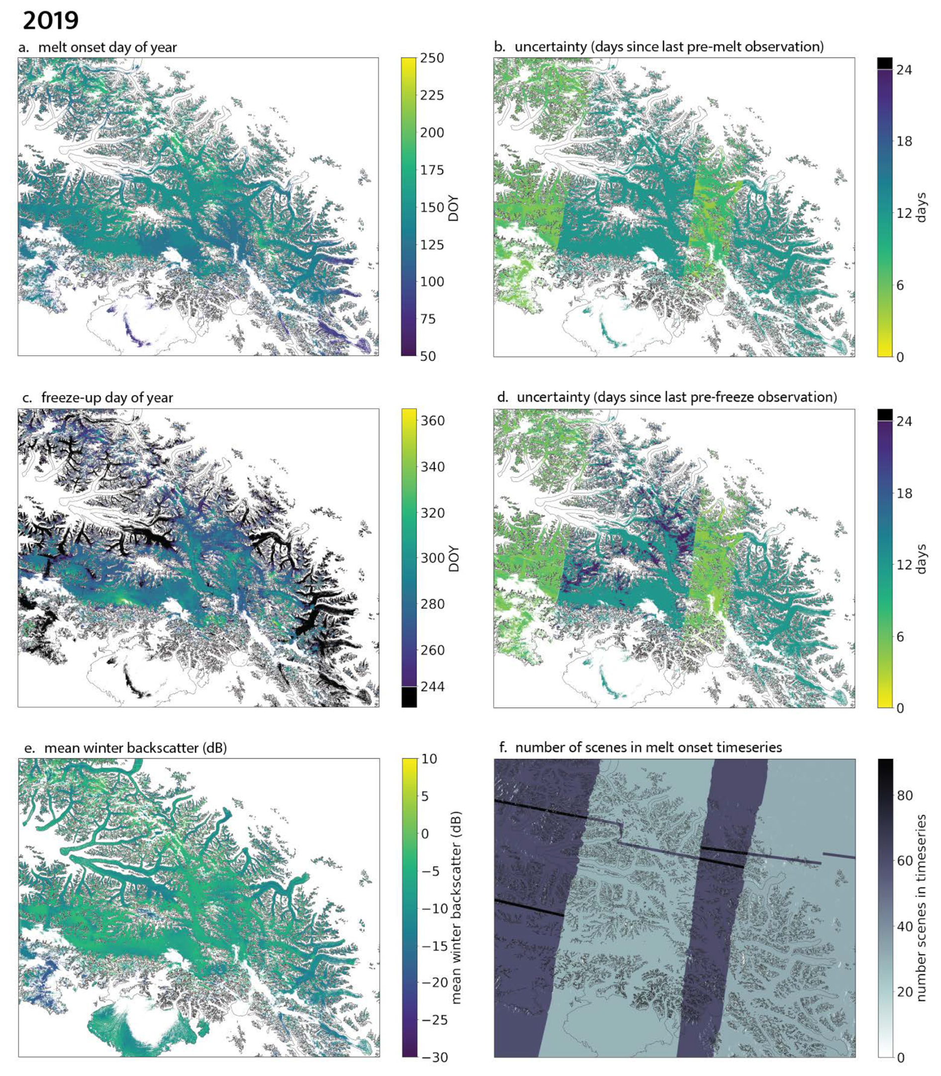
Figure E5 Melt onset (a), onset uncertainty (b), freeze-up (c), freeze-up uncertainty (d), mean winter backscatter (e), and number of scenes (f) over our study domain for 2019.

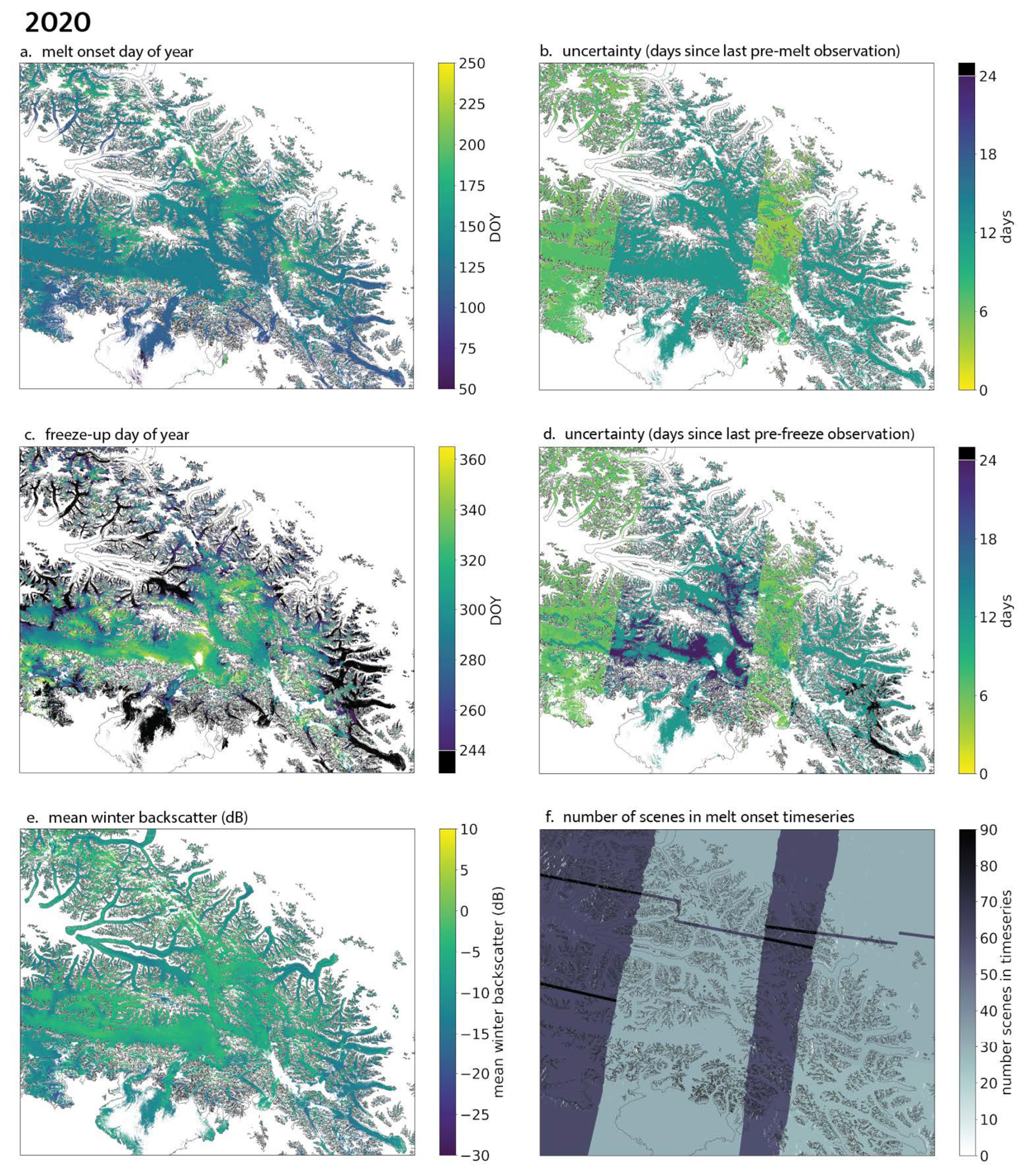
Figure E6 Melt onset (a), onset uncertainty (b), freeze-up (c), freeze-up uncertainty (d), mean winter backscatter (e), and number of scenes (f) over our study domain for 2020.

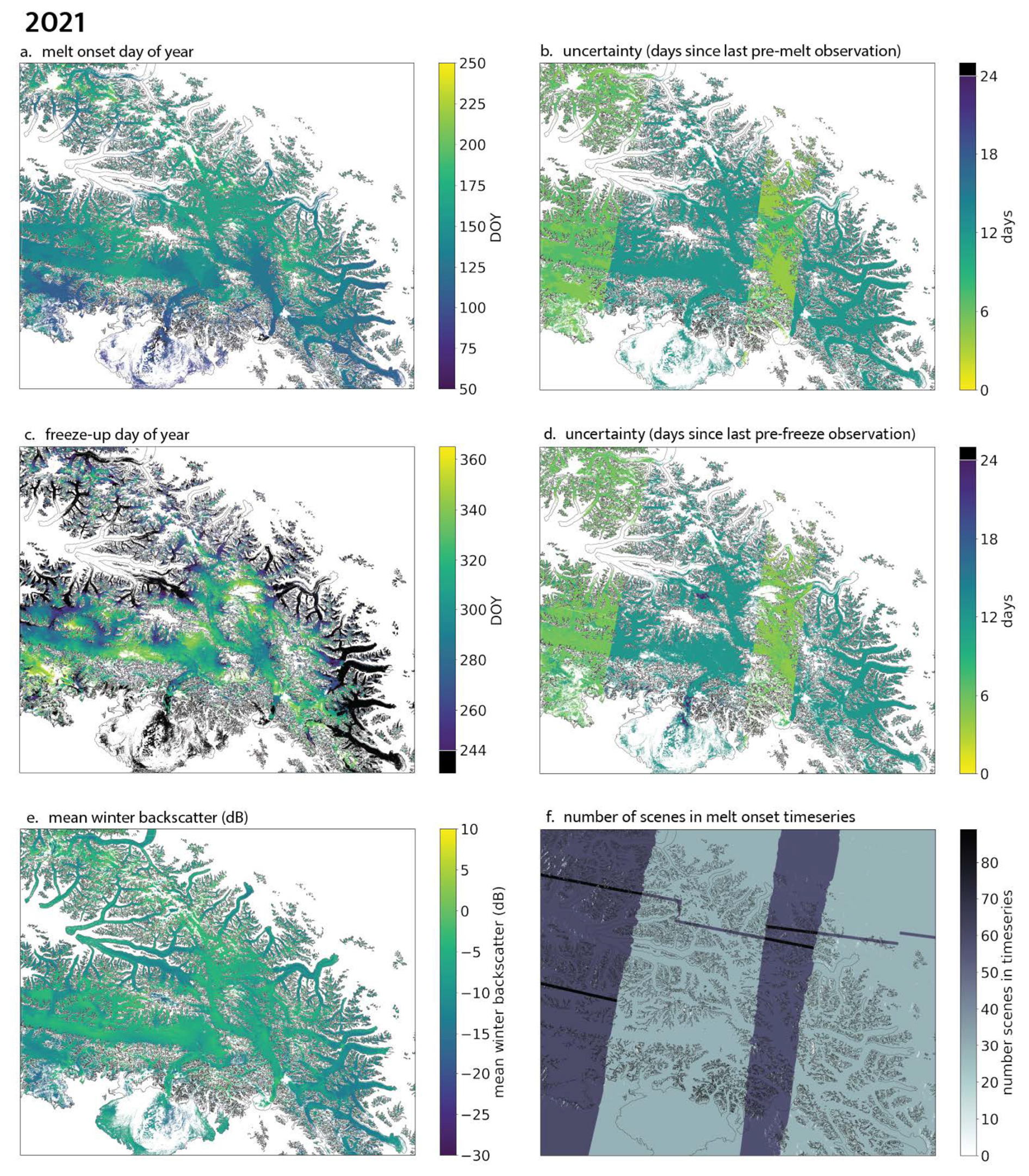
Figure E7 Melt onset (a), onset uncertainty (b), freeze-up (c), freeze-up uncertainty (d), mean winter backscatter (e), and number of scenes (f) over our study domain for 2021.

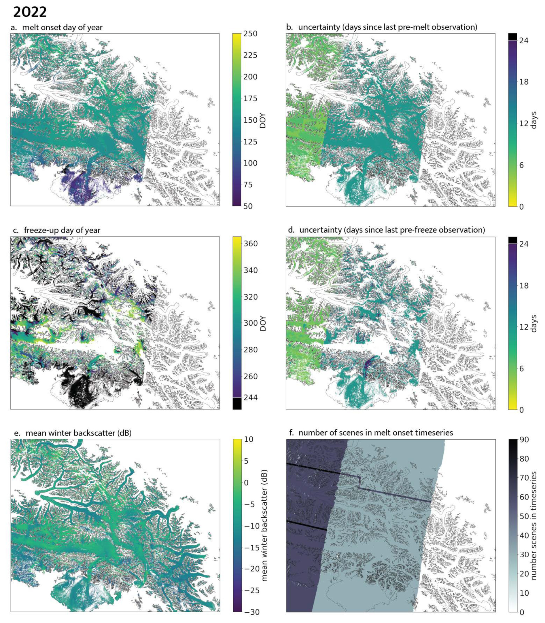
Figure E8 Melt onset (a), onset uncertainty (b), freeze-up (c), freeze-up uncertainty (d), mean winter backscatter (e), and number of scenes (f) over our study domain for 2022.

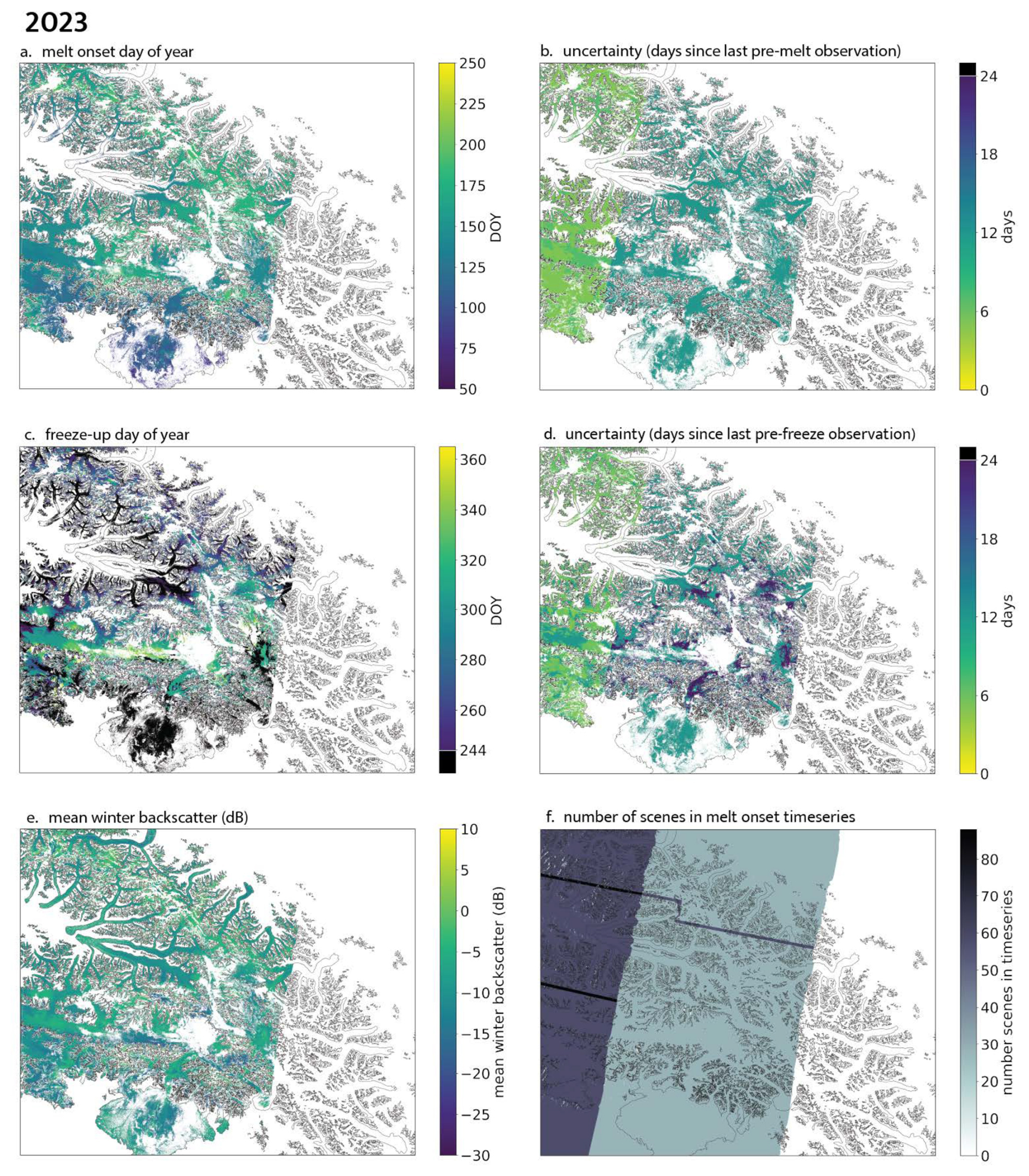
Figure E9 Melt onset (a), onset uncertainty (b), freeze-up (c), freeze-up uncertainty (d), mean winter backscatter (e), and number of scenes (f) over our study domain for 2023.

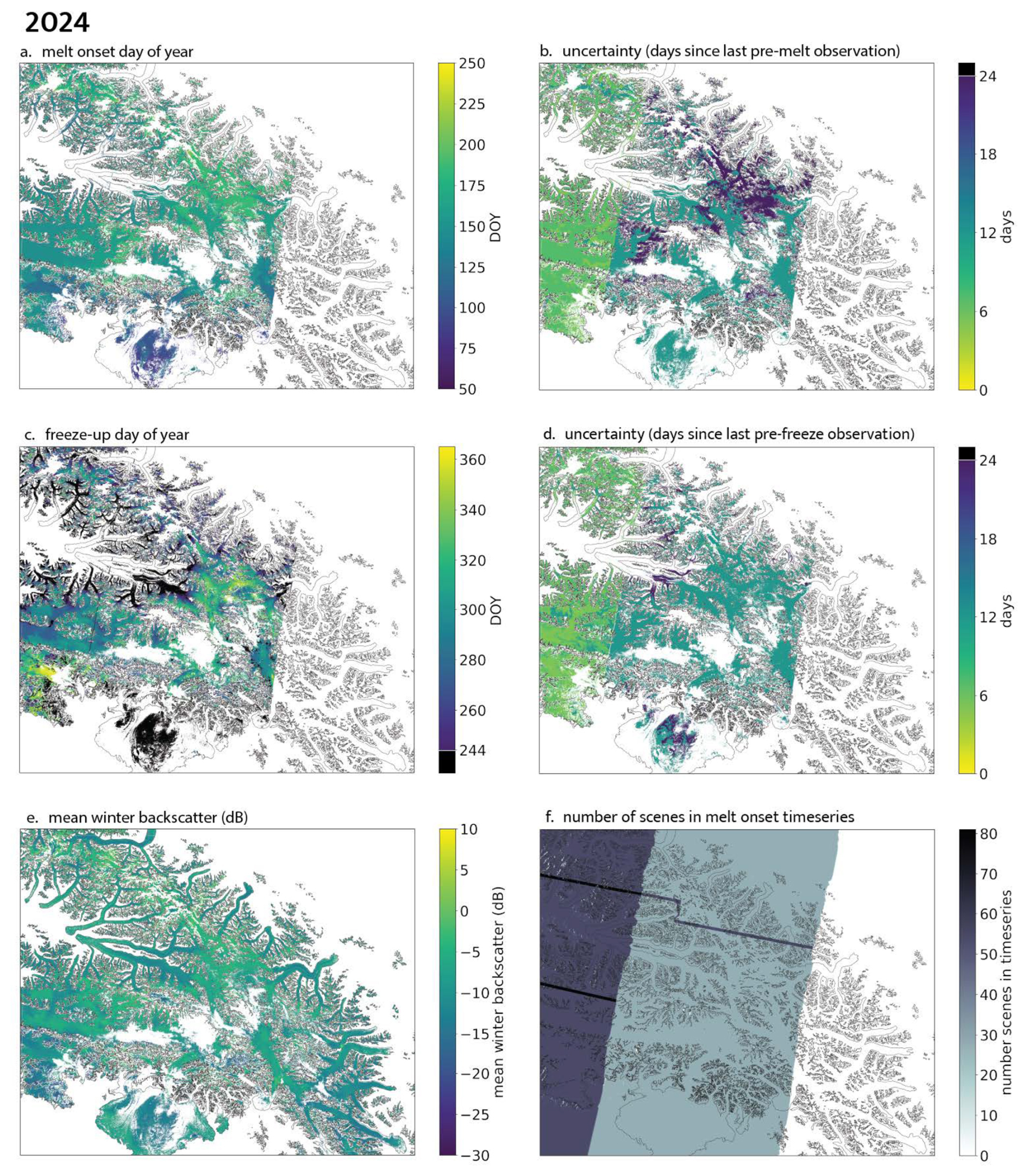
Figure E10 Melt onset (a), onset uncertainty (b), freeze-up (c), freeze-up uncertainty (d), mean winter backscatter (e), and number of scenes (f) over our study domain for 2024.

Appendix F: A comparison of melt onset with positive degree days

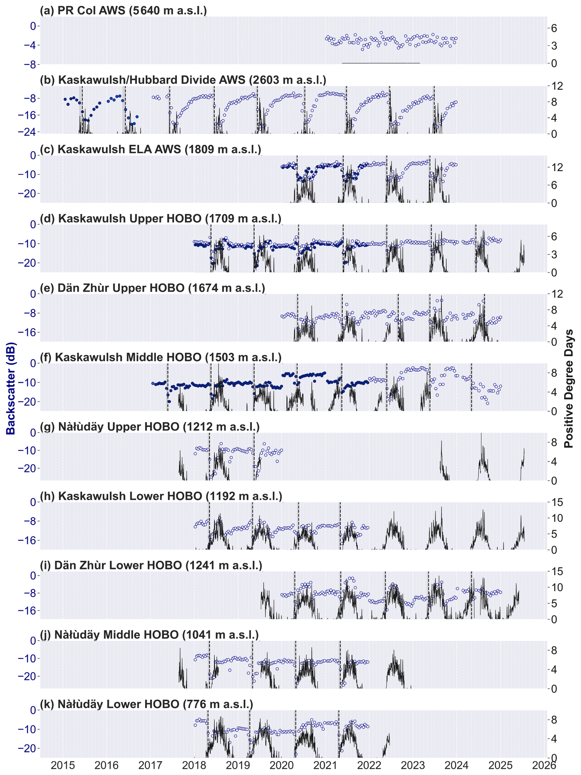
Figure F1 Sentinel-1 backscatter (blue circles) and positive degree days (black line) at calculated from air temperatures at automated weather station (AWS, panels a–c) and HOBO temperature logger (panels d–k) sites. Sites are shown from highest to lowest elevation. For sites with two overlapping path/frames, the backscatter timeseries for one is shown with open circles, while the backscatter timeseries for the other is shown with filled circles. SAR-derived melt onset day of year (DOY) is shown by the vertical dashed line, with the associated uncertainty (days) shown by the gray bar. Note that HOBO sensors are located on glacial ice, while AWS are located on bedrock nunataks (Fig. 1).