
the Creative Commons Attribution 4.0 License.
the Creative Commons Attribution 4.0 License.
 | 06 Oct 2026
A 2020 permafrost distribution map of the Qinghai-Tibet Plateau
Yuhong Chen

Wenbiao Tian
Yi Zhao
Shuping Zhao
Dongkai Yang
Guifei Jing
Fujun Niu
Permafrost on the Qinghai-Tibet Plateau (QTP) is undergoing rapid degradation, yet most existing distribution maps reflect long-term historical averages rather than the current thermal state of the ground. This temporal mismatch limits their usefulness for ecological, hydrological, and engineering applications. Here, we present a 1 km resolution permafrost distribution map for the 2020 period using an extended ground surface frost number model (FROSTNUM) driven by satellite-derived freezing/thawing indices. Because no concurrent field survey was available, we applied a space-for-time substitution strategy with Random Forest regression to estimate the empirical soil parameter (E) from environmental covariates. The resulting map shows that permafrost covered approximately 1.038 × 10⁶ km2 (39.35 % of the QTP), while seasonally frozen ground (SFG) covered 1.466 × 10⁶ km2 (55.57 %). Compared with the 2010 baseline, the permafrost area declined by 4.8 × 10⁴ km2 (a 1.82 % decrease). Degradation was spatially heterogeneous: the transition from permafrost to SFG was dominant in the central QTP, whereas the southern margin experienced substantial conversion of SFG to non-frozen ground. Validations against 109 independent borehole records yielded an overall accuracy of 0.84 and a Kappa of 0.58, outperforming existing 2020-period maps. This map provides a temporally specific reference for engineering risk assessment, ecological monitoring and the calibration of land surface models in this rapidly changing region.
- Article
(14887 KB) - Full-text XML
- BibTeX
- EndNote


Permafrost, defined as ground that remains below 0 °C for at least 2 consecutive years (Lewkowicz et al., 2025), underlies approximately 24 % of the exposed land surface in the Northern Hemisphere (Obu et al., 2019; Zhang et al., 1999). As a key component of the cryosphere, permafrost is highly sensitive to climate fluctuations and human interference (Burke et al., 2020; Chadburn et al., 2017; Smith et al., 2022). The Qinghai-Tibet Plateau (QTP), known as the “Third Pole” and “Asian Water Tower”, hosts the largest extent of permafrost in the mid- and low-latitude regions (Zhao et al., 2004). Owing to its unique high-altitude environment, QTP permafrost is characterized by relatively high temperatures and low thermal stability, making it particularly sensitive to warming (Li et al., 2008; Yang et al., 2019; Yao et al., 2022). Under ongoing global warming, permafrost degradation on the plateau has triggered profound impacts on regional hydrological processes (Tananaev and Lotsari, 2022), carbon cycling (Mu et al., 2020), ecosystem stability (Yang et al., 2010), and the safety of critical engineering infrastructure (Hjort et al., 2022). These wild-ranging impacts underscore the need for high-quality, up-to-date permafrost maps, which provide an essential foundational for quantifying environmental changes and supporting risk assessments in cold regions (Kim et al., 2024; Obu et al., 2019).
Although numerous permafrost maps of the QTP have been compiled (Guo and Wang, 2013; Zou et al., 2017), the evolution of mapping strategies reflects an ongoing struggle with data scarcity. Early maps were manually delineated on topographic bases using expert judgement and limited data sources, such as air temperature and field surveys (Cheng et al., 1996; Mi, 1990). While pioneering, these methods were inevitably subjective. Subsequent studies adopted empirical or semi-physical models for mapping, including altitude model (Li and Cheng, 1999), mean annual ground temperature (MAGT) model (Nan et al., 2002; Ran et al., 2022), frost number model (Nan et al., 2013; Shan et al., 2022), and the temperature at the top of permafrost (TTOP) model (Obu et al., 2019; Zou et al., 2017). To overcome the sparsity of in-situ observations, more recent semi-physical model studies have made extensive use of remote sensing and reanalysis datasets (Hachem et al., 2009; Zou et al., 2017). While these datasets help to fill the spatial gaps in ground station networks, they also introduce their own uncertainties. Remote sensing products, particularly land surface temperature (LST), are frequently plagued by cloud contamination, leading to significant data gaps (Yu et al., 2015). Conversely, reanalysis datasets, while spatially complete, often suffer from coarse spatial resolution and considerable uncertainty in complex terrain (Hu et al., 2019; Mao et al., 2010). More recently, physically-based land surface models (LSMs) (e.g. Zhang et al., 2019; Zhao et al., 2022) and machine learning approaches (e.g. Ni et al., 2021; Ran et al. 2021) have been used to capture complex process mechanisms and non-linear relationships. While LSMs can in principle simulate temporal evolution, they carry considerable uncertainty when upscaled to the heterogeneous QTP without extensive calibration, and purely data-driven machine learning models often suffer from spatial biases owing to the lack of representative training data across the vast plateau (Gay et al., 2023; Siewert, 2018).
Beyond these data limitations, a fundamental temporal deficiency persists across most existing products (Obu et al., 2019; Zou et al., 2017): they largely reflect long-term historical averages rather than the current distribution of frozen ground. Because ground observations on the QTP are sparse and unevenly distributed, concentrated mostly along transportation corridors, previous mapping efforts often pooled data across multiple decades to increase sample size (Ran et al., 2012). As a result, these maps depict a composite state that smooths over the rapid climatic shifts of past decades. This reliance on climatological averages creates a temporal mismatch that hinders the accurate validation of land surface models and ecological assessments that require precise, period-specific benchmarks (Cao et al., 2023).
To address the need for a temporally specific benchmark, our previous work (Cao et al., 2023) developed a high-quality permafrost distribution map for 2010. That study employed an extended ground surface frost number model (FROSTNUM), incorporating cloud-gap-filled satellite freezing/thawing indices and an empirical soil parameter (E) calibrated against extensive survey data from the 2009–2010 period. It provided the first period-specific benchmark of the QTP permafrost distribution and has been widely used since its publication (e.g. Deng et al., 2024; Pan et al., 2024; Zhong et al., 2024).
However, the climate on the QTP has changed rapidly over the 2010–2020 decade (Hu et al., 2024; Zhao et al., 2025), so the 2010-period map is now increasingly outdated for contemporary applications. Producing a comparable map for the 2020 period is not straightforward, however, because the extensive field surveys carried out for 2010 were not repeated in 2020. To fill this gap, we present a new, high-accuracy 1 km QTP permafrost map of the QTP for the 2020 period. We refine the FROSTNUM mapping framework (Cao et al., 2023; Hu et al., 2020) by introducing a space-for-time substitution strategy. We hypothesize that although the climatic drivers (freezing and thawing indices) have shifted, the underlying statistical relationship between the empirical soil parameter (E) and environmental covariates (e.g., topography, soil texture, vegetation, and soil moisture) remains sufficiently stable over a decadal interval to support meaningful extrapolation. By training machine learning models on the high-quality 2010 E field and driving them with updated 2016–2020 environmental conditions, we derived the E parameter for the 2020 period. The resulting map provides an up-to-date dataset for quantifying decadal permafrost changes and supporting future high-precision modeling on the QTP.
2.1 Study area
The QTP, widely known as the “Third Pole” and the “Asian Water Tower”, is the highest and most extensive plateau on Earth. Located between 26–40° N and 73.5–104.5° E, it spans an area of approximately 2.5 × 10⁶ km2 with an average elevation exceeding 4000 m above sea level (a.s.l.) (Fig. 1). As the headwaters of major Asian river systems, including the Yangtze, Yellow River, Indus, Mekong, and Ganges, the plateau plays a key role in the regional hydrological cycle and sustains water resources for downstream populations.
The plateau is characterized by a distinctive high-altitude cryospheric environment, with extensive distribution of glaciers, snow cover, and permafrost (Qiu, 2008; Yao et al., 2012).The climate is governed by the interplay between the westerlies and the Asian monsoon, creating a pronounced climatic gradient. Mean annual air temperature generally ranges from −5 and 5 °C (Zhang et al., 2019), while mean annual precipitation decreases from over 700 mm in the humid southeast to less than 50 mm in the arid northwest (Peng et al., 2019). Approximately 70 % of annual precipitation occurs during the monsoon season from May to September (Kukulies et al., 2020; Zhu et al., 2020).
Vegetation cover transitions from alpine forests and meadows in the southeast to alpine steppes and deserts in the northwest (Zhou et al., 2025). Permafrost thickness varies accordingly, ranging from a few meters in marginal zones to approximately 350 m in the interior, with the depth of zero annual amplitude typically varying between 3.5 to 17 m (Zhao et al., 2020). The QTP is experiencing rapid climate warming. Between 1960 and 2015, the annual mean temperature rose at a rate of 0.33 °C per decade, more than double the global warming rate (0.14 °C per decade) (Zhang et al., 2020). This accelerated warming has intensified cryospheric instability, underscoring the need for up-to-date monitoring of permafrost distribution.
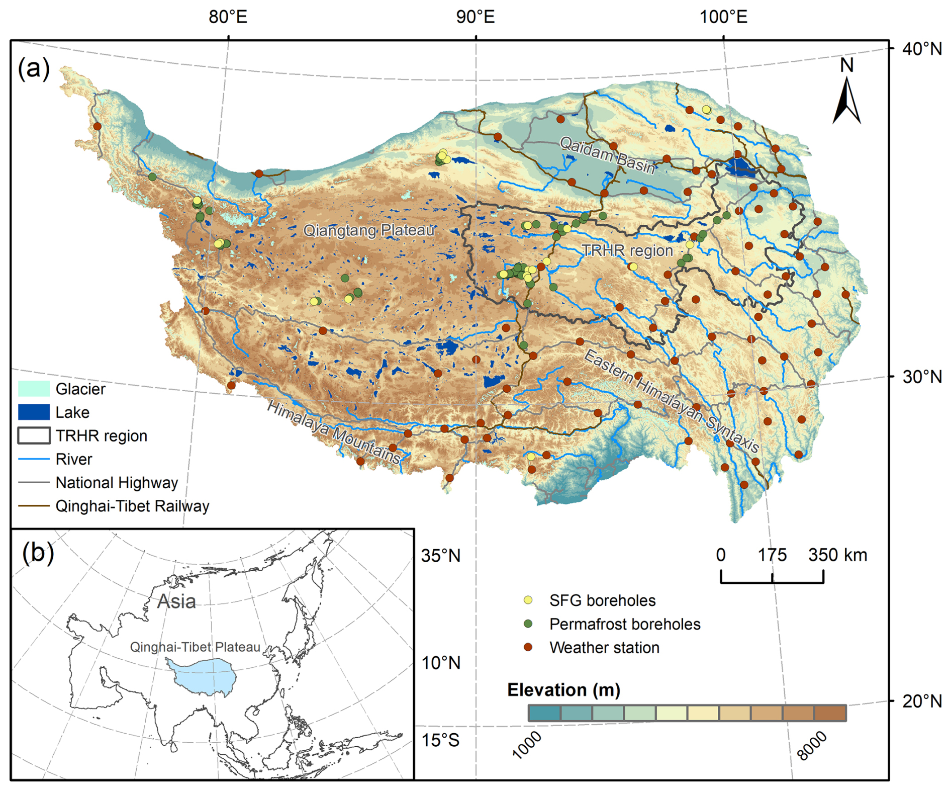
Figure 1Topographic map and geographical context of the Qinghai-Tibet Plateau (QTP). (a) The topography of the region. The background color gradient represents elevation derived from the Shuttle Radar Topography Mission DEM. The 87 national meteorological stations (red dots) used for ground surface temperature correction are shown, alongside major river systems and lakes. Notably, the 83 permafrost boreholes and 26 seasonally frozen ground (SFG) boreholes for validation are largely concentrated in the Three-River Headwater Region (TRHR) and surrounding headwater areas. (b) The location of the QTP in Asia.
2.2 Remote sensing and gridded datasets
2.2.1 Thermal forcing data
The freezing and thawing indices are the primary drivers of permafrost thermal dynamics in our model. To derive these indices, we used the Moderate Resolution Imaging Spectroradiometer (MODIS) LST products as the basis for estimating ground surface temperature (GST). We acquired the Version 6 Terra (MOD11A1) and Aqua (MYD11A1) daily LST products, which provide four observations per day at a 1 km spatial resolution.
To determine the permafrost distribution for the 2020 period, we processed data covering the 5-year period from 2016 to 2020. This temporal selection satisfies the definition of permafrost (ground remaining frozen for at least 2 years) and minimizes the bias from interannual climate anomalies. Because raw satellite skin temperatures differ from the ground surface thermal regime required by the model, these data were post-processed. This included a dedicated gap-filling procedure to address cloud contamination (Chen et al., 2023) and a subsequent LST-to-GST correction to account for the thermal buffering effects of vegetation and snow. The specific algorithms for these transformations are detailed in Sect. 3.2.
2.2.2 Data for estimating local soil parameter (E)
While regional thermal dynamics are governed by temperature indices, local permafrost occurrence is strongly modulated by surface and subsurface characteristics. In our model (Sect. 3.1), these local effects are aggregated into an empirical soil parameter E. To estimate E, we compiled environmental covariates representing topography, surface cover, soil properties, and moisture conditions (Karjalainen et al., 2019; Smith et al., 2022).
Topographic variables (slope, aspect, and topographic wetness index (TWI)) were derived from the Shuttle Radar Topography Mission (SRTM) 90 m Digital Elevation Model (DEM), aggregated to 1 km resolution to match the model grid. Surface cover conditions were characterized using the 1 km, 16 d composite MODIS Normalized Difference Vegetation Index (NDVI) product (MOD13A2) and the daily 0.005° fractional snow cover (FSC) dataset over High Asia (Pan et al., 2024).
Subsurface thermal properties were represented by soil texture data (sand and clay fractions) extracted from the China Dataset of Soil Properties for Land Surface Modeling (Shangguan et al., 2013). Because high-resolution soil moisture products are not available, we used mean annual precipitation (MAP), derived from the 1 km monthly precipitation dataset for China (Peng et al., 2019), as a proxy for regional soil moisture conditions. All dynamic covariates (NDVI, FSC, and MAP) were averaged over the 2016–2020 period.
2.3 In situ observations
2.3.1 Meteorological station data
To correct the thermal offset between satellite-derived LST and the actual ground thermal regime, we utilized daily 0 cm GST observations from the Daily Meteorological Dataset of Basic Meteorological Elements of China National Surface Weather Station (1991–2020) (Zhao et al., 2024). The original dataset includes 131 stations across the QTP. We screened these stations based on the completeness of their data series, excluding sites with significant missing records during the 2016–2020 period. This resulted in a final subset of 87 stations utilized for this study (Fig. 1). Daily GST records from 2016–2020 were extracted to correspond with the satellite acquisition period.
2.3.2 Borehole observations
We validated the mapped permafrost distribution independently using a compilation of 109 borehole records. Because deep ground temperature measurements coinciding exactly with 2020 are limited, we prioritized high-quality observations from the years immediately surrounding 2020, on the assumption that deep ground thermal states remain relatively stable over such short timeframes. The primary data source was the comprehensive QTP permafrost thermal state synthesis by Zhao et al. (2021). From this dataset, we extracted records for 65 boreholes where ground temperatures were monitored at depths of 10 and 20 m. We utilized the 2018 ground temperatures as the reference. Sites with MAGT < 0 °C at these depths were classified as permafrost.
To improve spatial coverage, we integrated three additional regional datasets: (1) 32 boreholes from the Yangtze River Source area (Li et al., 2022) with direct presence/absence observations specifically for the year 2020; (2) 6 boreholes from the Yellow River Source area (Lei et al., 2024), classified using 2017 ground temperature profiles (0–20 m); and (3) 6 sites from the Heihe River Basin observation network (Mu et al., 2022) covering the northeastern QTP, all of which are situated in seasonally frozen ground (SFG) regions (based on records from 2011–2019). In total, the validation dataset comprises 83 confirmed permafrost sites and 26 seasonally frozen ground sites, providing a spatially diverse basis for accuracy assessment.
2.4 Datasets for comparison and land cover consistency
To evaluate the accuracy of our new map, we compared it against two existing permafrost datasets that cover the 2020 period. The first is the TTOP-based permafrost map (Yan et al., 2023). This map is derived from a long-term permafrost simulation dataset (1961–2020) generated at a 5-year interval using the TTOP model (Smith and Riseborough, 1996) driven by satellite LST and meteorological station observations. For this study, we extracted the permafrost distribution for the 2020 period, at its native 1 km spatial resolution.
The second dataset is a MAGT-based permafrost map derived from a ground temperature simulation product (Zou et al., 2025). This dataset provides MAGT at a depth of 15 m for the period 2010–2019, generated using a Support Vector Machine model trained on records from 231 boreholes. For comparison, grid cells with a 15 m ground temperature below 0 °C were classified as permafrost.
To keep land cover definitions consistent across the compared maps, we used glacier extent data from Ye et al. (2017) and 2020 lake boundaries from Zhang et al. (2021) to exclude non-soil areas.
3.1 The extended FROSTNUM/COP model framework
We mapped the 2020-period permafrost distribution using the FROSTNUM model (Cao et al., 2023; Hu et al., 2020). This semi-physical approach, previously validated for the QTP by Cao et al. (2023), estimates the probability of permafrost occurrence (frost number F) from the balance between surface freezing and thawing loads, as modulated by local ground properties. The frost number F is defined as:
where DDF and DDT are the ground surface freezing and thawing indices (°C ⋅ d), respectively. The parameter E is a dimensionless empirical factor that captures local environmental modification of the ground thermal regime. Theoretically, E reflects the combined effects of soil thermal properties and moisture conditions in both frozen and thawed states. Based on this formulation, the threshold for permafrost occurrence is defined at F>0.5. Pixels with F≤0.5 are classified as SFG or non-frozen ground (Hu et al., 2020). The threshold F=0.5 is physically meaningful because it represents the point at which the potential freezing and thawing effects are balanced. When F>0.5, the freezing effect dominates over the thawing effect, allowing the ground to remain frozen throughout the year and thus indicating permafrost. When F≤0.5, the thawing effect equals or exceeds the freezing effect, meaning the ground thaws completely during the warm season and is therefore classified as SFG (or non-frozen ground).
A critical component of this framework is the determination of E. In the original methodology established (Cao et al., 2023; Hu et al., 2020), the E parameter was retrieved via an inverse optimization strategy that minimized the error between the model output and extensive concurrent field survey maps. This ensured that the 2010 map accurately reflected ground conditions specific to that year. However, this original strategy cannot be applied directly for 2020, since it depends on concurrent permafrost survey maps for calibration, and no such maps exist for the 2020 period. To overcome this limitation, we instead adopt a space-for-time substitution strategy, on the hypothesis that although the specific value of E at a given location may shift with changes in moisture or surface cover, its fundamental statistical relationship with environmental drivers (topography, vegetation, soil texture, soil moisture) remains applicable over a decadal scale. This allows us to predict the 2020 E field from relationships learned from the high-quality 2010 dataset (Fig. 2). More specifically, we used the high-quality 2010 E distribution map produced by Cao et al. (2023) and applied two transfer learning strategies, a neural network approach and a random forest (RF) approach, to establish the relationships between E and multiple environmental drivers. By updating the environmental drivers to their 2016–2020 values, we derived the predicted E values for the 2020 period from these learned statistical relationships. Further details on the estimation of the soil parameter E for the 2020 period are provided in Sect. 3.3.
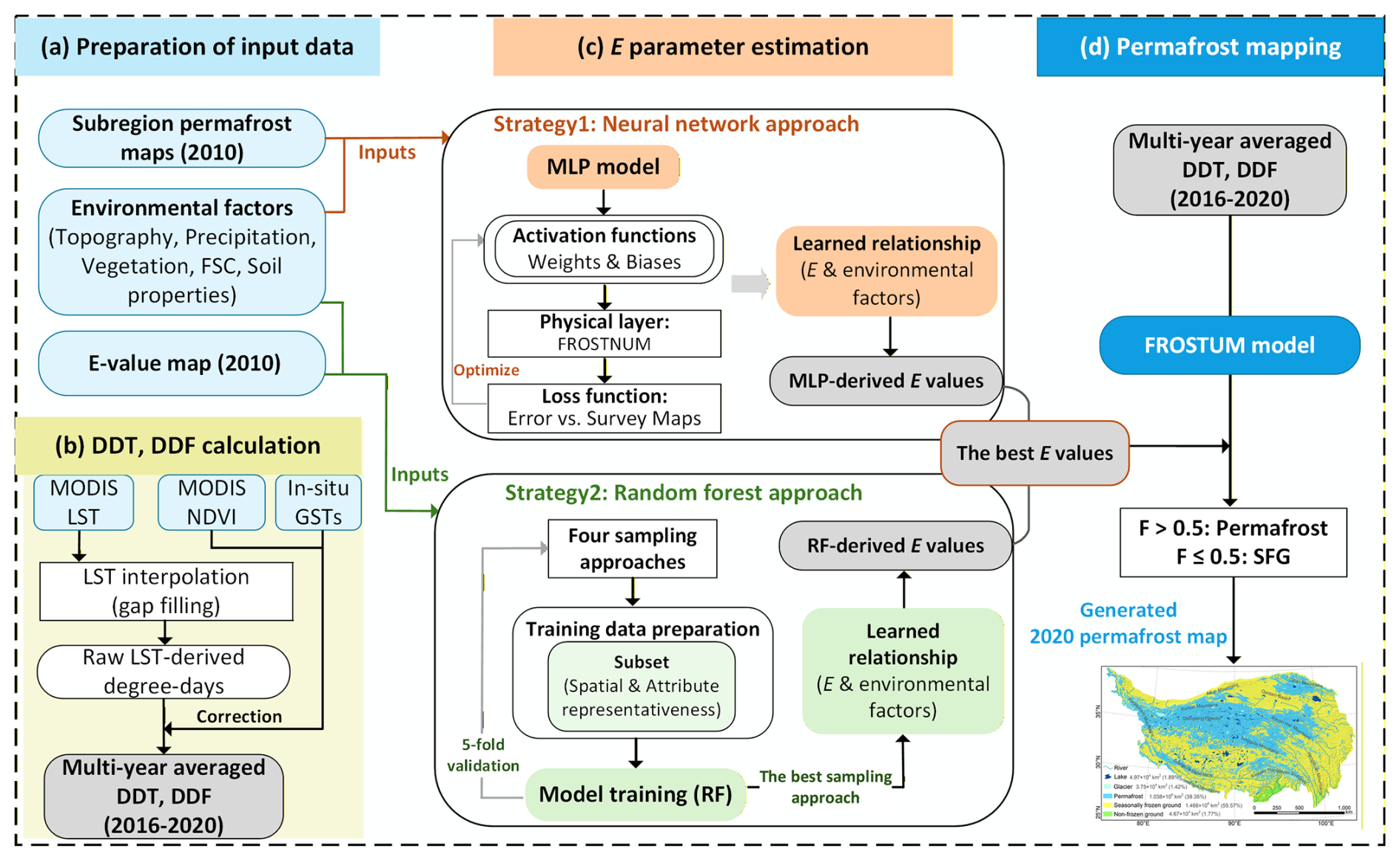
Figure 2Schematic flowchart of the methodology to map the 2020-period permafrost distribution. The workflow comprises four distinct stages: (a) preparation of multi-source input datasets, including satellite forcing data and environmental covariates; (b) calculation of ground surface freezing (DDF) and thawing (DDT) indices from gap-filled MODIS land surface temperature (LST), corrected to represent ground surface conditions; (c) estimation of the empirical soil parameter E via a space-for-time substitution strategy. This stage compares two transfer learning approaches: a neural network (MLP) approach and a Random Forest (RF) regression with optimized spatial sampling; and (d) final permafrost distribution mapping using the extended ground surface frost number model (FROSTNUM). FSC: fractional snow cover; MODIS (Moderate Resolution Imaging Spectroradiometer); GST: ground surface temperature; NDVI: normalized difference vegetation index; SFG: seasonally frozen ground; and MLP: multilayer perceptron model.
3.2 Calculation of ground surface freezing and thawing indices
The driving variables for the model, DDF and DDT, were derived from the daily MODIS LST products (MOD11A1 and MYD11A1) covering the 2016–2020 period. The processing workflow comprised gap-filling, daily aggregation, and the correction from LST to GST. Because cloud cover is frequence on the QTP, raw MODIS LST data suffer from extensive gaps. We addressed this using the solar-cloud-satellite geometry interpolation method developed by Chen et al. (2023). This approach reconstructs missing pixels using the geometric relationship between the sun, cloud position, and satellite view angle, yielding high-accuracy all-weather LST estimates. Following gap-filling, the daily mean LST was calculated from the four daily instantaneous observations (two daytime and two nighttime) using a sinusoidal integration method (van Doninck et al., 2011).
The raw surface freezing and thawing indices were then computed from the gap-filled daily mean LST series. DDF was calculated as the annual sum of negative degree-days. For DDT, a correction was needed to account for the thermal offset between satellite-observed LST and actual GST, caused primarily by the insulating effect of vegetation during the growing season. Consistent with Cao et al. (2023), we corrected the LST-derived DDT using a multilinear regression model (Eq. 2) that incorporates vegetation greenness and latitude. The correction is applied at 16 d intervals (corresponding to MODIS NDVI composites) to derive a final annual DDTGST:
where DDTi,GST represents the corrected ground surface thawing degree-days (°C ⋅ d) for the ith temporal interval (corresponding to the 16 d MODIS composites period); DDTi,LST is the raw thawing degree-days accumulated from positive daily mean LST values during the same ith interval, NDVIi is corresponding NDVI value, serving as a proxy for vegetation density and its thermal insulating capacity; and Lat is the geographic latitude, which accounts for regional variations in solar radiation and incidence angle. No correction was applied to DDF, as snow cover on the QTP is thin, ephemeral, spatially discontinuous, resulting in a negligible insulation effect at the regional scale (Wu and Zhang, 2008; Zhao et al., 2017).
3.3 Estimation of soil parameter E via space-for-time substitution
We used a space-for-time substitution strategy to obtain E for the 2020 period in the absence of concurrent field surveys. This approach is well established in Earth system sciences, particularly climatology, atmospheric modeling, and ecology, where spatial gradients are routinely used to infer temporal dynamics or parameterize processes in data-scarce settings (Huang et al., 2019; Pickett, 1989). In the context of this study, we assume that while the specific value of E at a location may shift with changes in soil moisture or surface cover, the statistical dependencies between E and environmental covariates (soil texture, topography, and vegetation-moisture proxies) observed in 2010 remain valid for predicting the 2020 state. To this end, we developed and compared two distinct transfer learning strategies, each prioritizing a different source of training data. Both strategies utilized the same suite of predictors to estimate E, specifically: topographic variables (elevation, slope, aspect, TWI), soil texture (sand and clay fractions), vegetation conditions (NDVI), snow cover (FSC), and precipitation (MAP).
The first strategy learned the E-environment relationship directly from the high-reliability field survey maps available for five sub-regions in the 2010 study. We constructed a hybrid physics-informed neural network (Fig. 2c). This architecture integrates a Multi-Layer Perceptron (MLP) (Fu et al., 2025; Park and Lek, 2016) with the physical FROSTNUM model in an end-to-end differentiable framework. In the forward pass, the MLP predicts the local parameter E from environmental inputs, which is immediately passed through the differentiable FROSTNUM layer to calculate the frost number and subsequent binary classification. In the backward pass, the generated classification is compared directly against the survey maps, and the classification error is backpropagated through the physical layer to update the MLP weights.
The second strategy prioritized spatial continuity and statistical robustness, using the full 2010 E-field retrieved via the original Clustering-Optimization-Prediction procedure (Cao et al., 2023) as the training target. Unlike the first strategy, which relied on sparse survey data, this approach treated the estimation of E as a direct regression problem against the spatially continuous 2010 baseline map. We trained a RF model (van Der Westhuizen et al., 2023; Wadoux et al., 2019) to learn the relationships between the environmental covariates and these “observed” E values. While the original study aggregated the plateau into eight parameter clusters, we expanded this to sixteen classes for the training target.
For the second strategy, we also implemented a representative sampling framework to select the training data. Given the high spatial heterogeneity of the QTP, simple random sampling often fails to capture rare but physically significant parameter combinations, which increases predictive uncertainty. We evaluated four distinct sampling techniques: k-means clustering sampling (Brus et al., 2006), Equal Range (ER) sampling (Hengl et al., 2003), Principal Component Analysis (PCA)-based sampling (Hengl et al., 2003), and Latin Hypercube Sampling (LHS) (Carré et al., 2007) across four different sample sizes (1000, 3000, 5000, and 10 000 points) using 5-fold cross-validation. Our aim was not only to improve computational efficiency and reduce information redundancy, but, more importantly, to minimize the uncertainty in the E-value distribution. Detailed mathematical formulations and implementation procedures for these four sampling strategies are provided in Appendix A. The configuration with the best performance was then selected to generate the E map for the 2020 period. Details of the accuracy comparison among the different sampling strategies are provided in Sect. 4.2.
3.4 Validation and uncertainty analysis
We evaluated the accuracy and reliability of the resulting 2020-period permafrost map through a multi-tiered validation framework that assessed both the intermediate modeling steps and the final spatial product. First, we conducted a comparative evaluation of the MLP and the RF strategies described in Sect. 3.3 to determine the optimal transfer learning strategy for estimating E. For the RF approach, we used 5-fold cross-validation to assess its ability to reproduce the 2010 baseline values, quantifying performance using the correlation coefficient (r), mean absolute error (MAE), root mean square error (RMSE), and percentage of variance explained. For the MLP approach, the MLP performance was validated indirectly by assessing the classification accuracy of the simulated permafrost distribution in the target subregions. Specifically, we randomly selected 70 % of the pixels within these subregions for training, while the remaining 30 % were reserved for validation. We also assessed the spatial consistency of the MLP-derived 2010 permafrost distribution by comparing it with the benchmark map from Cao et al. (2023).
Second, we carried out a two-part validation, assessing both the accuracy of the 2020 map and the plausibility of the detected temporal changes. The spatial accuracy of the resulting 2020 permafrost distribution, generated using the selected optimal strategy, was assessed against the independent dataset of 109 borehole records. To perform this evaluation, we extracted the simulated permafrost status (permafrost or SFG) at the coordinates of each borehole and compared it with the in-situ ground truth. Beyond this static accuracy, we also checked the plausibility of the simulated 2010-2020 permafrost changes using 0 cm GST data from meteorological stations and available field evidence.
We also assessed the map's consistency with current regional knowledge through a spatial inter-comparison with two existing datasets covering the same period: the TTOP-based simulation by Yan et al. (2023) and the data-driven ground temperature map by Zou et al. (2025). We quantified agreement in permafrost area and spatial distribution patterns, focusing on discrepancies in the zones where modeling uncertainty is typically highest. Finally, to diagnose the physical drivers underlying these shifts, we compared key environmental and thermal variables between changed areas and adjacent unchanged regions.
Third, we conducted a systematic uncertainty analysis for both the soil parameter E and the final permafrost map, to quantify the uncertainty arising from the choice of training sample selection. A 16-member ensemble was constructed by cross-combining four sampling strategies and four sample sizes. The stability of the predicted E values was evaluated using the ensemble mean, standard deviation, and coefficient of variance (CV). The propagation of this uncertainty into the final classification was assessed by analyzing variations in simulated permafrost areas and by mapping the permafrost agreement probability (Pagree), which delineates stable zones from zones of classification inconsistency. The results of this uncertainty analysis are presented in Appendix C and Sect. 4.4.1.
4.1 Spatiotemporal changes in thermal forcing
The thermal forcing indices driving the permafrost model showed distinct spatial shifts between the 2010 baseline and the 2020 period. The DDT, corrected to account for the thermal offset between satellite-observed skin temperature and the actual ground surface, revealed a spatially divergent pattern (Fig. 3a–c). As shown in the relative difference map (Fig. 3c), significant warming persisted in the arid northern Qaidam Basin and the western Qiantang Plateau, where sparse vegetation offers limited thermal buffering. In contrast, a slight cooling trend was observed across parts of the eastern QTP. Analysis of the raw LST-derived DDT indicates that most of the Three-River Headwater Region (TRHR) experienced slight warming, whereas the vegetation- and latitude-corrected DDT shifts the signal toward slight cooling in this region. The magnitude of this cooling is generally small, with relative differences mostly within ±5 % across the central TRHR and reaching 5 %–15 % in the eastern margin of the plateau. The localized cooling is likely attributable to the greening of the plateau, a phenomenon well-documented in the southeastern QTP over recent decades (Shi et al., 2023; Wang et al., 2022). Vegetation modulates the surface energy budget through three primary mechanisms: (1) reducing aerodynamic resistance and enhancing latent heat flux via evapotranspiration; (2) increasing soil water retention, which raises the thermal inertia of the soil; and (3) providing direct insulation that delays the onset of active-layer thaw (Jia et al., 2023; Ni et al., 2025; Wang et al., 2012). This interpretation is supported by local meteorological stations observations: 6 of 8 stations in the eastern margin of the TRHR recorded a decreasing trend in DDT during 2016-2019. This ground-based evidence indicates that the cooling signal is not merely an artifact of the satellite LST correction, but reflects a genuine change in surface thermal conditions.
The DDF reflected these regional climatic contrasts (Fig. 3d–f). Between 2010 and 2020 periods, pronounced winter warming (manifested as reduced DDF in Fig. 3f) occurred across the central QTP and was particularly intense along the southern Himalayan margin. Conversely, localized cooling (increased DDF) was observed in the western QTP and the eastern mountainous regions (Fig. 3f). As a result, the DDT-to-DDF ratio (DDT DDF), a key climatic indicator of permafrost stability, increased markedly across the majority of the QTP from the 2010 to the 2020 period (Fig. 3g–i). This positive shift signals a climate trajectory unfavorable for permafrost preservation in these regions. However, the eastern region showed a decrease in the DDT DDF ratio, consistent with the observed DDT and DDF cooling trend.
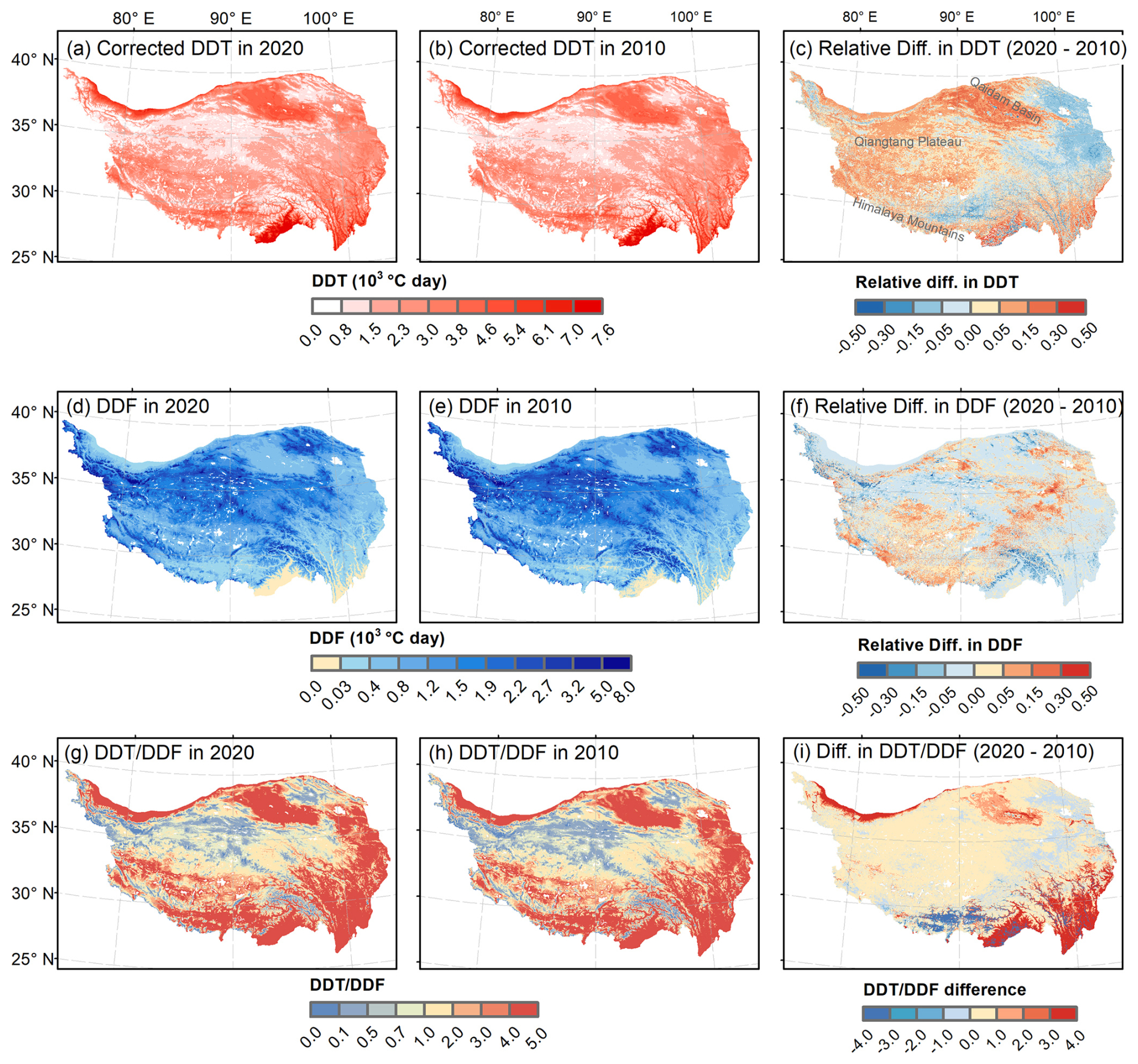
Figure 3Spatial distribution and decadal changes of thermal forcing indices on the QTP. (a–c) DDT and its relative changes, (d–f) DDF and its relative changes. (g–i) Ratio of thawing to freezing indices (DDT DDF) and its decadal change. The left and middle columns present the spatial distribution for the 2020 period and 2010 period, respectively. The right column shows their decadal differences. The relative differences in (c) and (f) are calculated using baseline denominators of 2000 and 1200 °C ⋅ d, respectively, which are the regional mean values of DDT and DDF averaged across both periods. For panels (c) and (i), positive values (red) indicate warming/instability, while negative values (blue) indicate cooling/stability. For panel (f), negative values (red) indicate winter warming (reduced freezing), while positive values (blue) indicate cooling.
4.2 Estimation of the soil parameter E for the 2020 period
To estimate the empirical soil parameter E for the 2020 period, we applied a space-for-time substitution strategy using two transfer learning approaches trained on the high-quality 2010 E field from Cao et al. (2023). While the MLP model achieved high accuracy (95.26 %) within the training subregions, it overfit severely when applied across the entire plateau. The MLP-predicted E field showed unrealistic spatial artifacts and failed to reproduce the benchmark 2010 permafrost distribution of Cao et al. (2023) (see Appendix B for details). This suggests that unconstrained neural networks may lack sufficient physical constraints for robust spatial extrapolation in heterogeneous environments such as the QTP.
The RF-based approach, in contrast, generalized much strongly. Among four sampling strategies evaluated through 5-fold cross-validation, the k-means clustering sampling method with 5000 points performed best, achieving an RMSE of 0.048, MAE of 0.029, and explaining 74.83 % of the variance in the 2010 E field (Table 1). This configuration was therefore adopted to generate the E map for the 2020 period.
Figure 4 presents the spatial distribution of E in the 2020 period and the reference 2010. The overall spatial pattern remains broadly consistent between the two periods, although regional differences are evident. Areas with increased E (positive group) account for 55 % of the total changed area, while areas with decreased E (negative group) account for 45 %. Regions with rising E are located mainly in the central and northern plateau, whereas declining E values are more scattered, especially along the eastern and southern margins (Fig. 4c).
To further test the robustness of the predicted E values, we performed an ensemble analysis using 16 combinations of sampling strategies and sample sizes (Appendix C). The results indicate a high level of consistency. The CV of E remains below 5 % across 98.5 % of the QTP, suggesting that the spatial pattern of E in the 2020 period is relatively stable with respect to the choice of training sample selection.
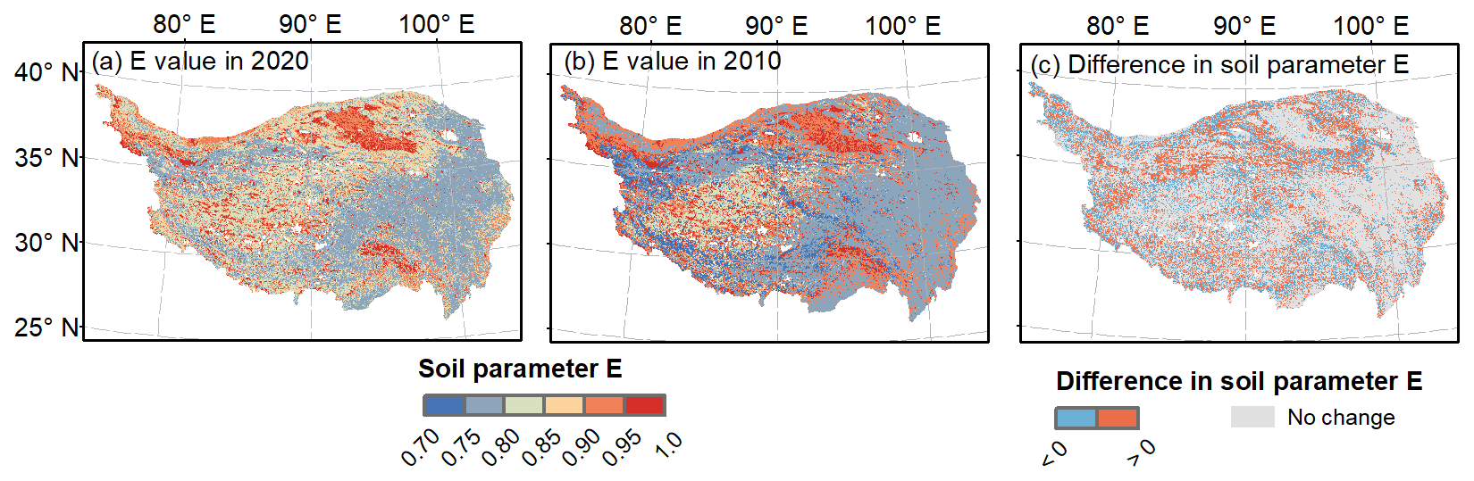
Figure 4Spatial distribution of the soil parameter E in the 2020 period (a) and 2010 (b). (c) illustrates the difference (2020 minus 2010), where positive values (red) indicate an increase in E (conditions conducive to degradation) and negative values (blue) indicate a decrease. The 2010 E map was derived from Cao et al. (2023), whereas the 2020-period E map was predicted using a space-for-time substitution strategy.
4.3 The 2020-period permafrost distribution map
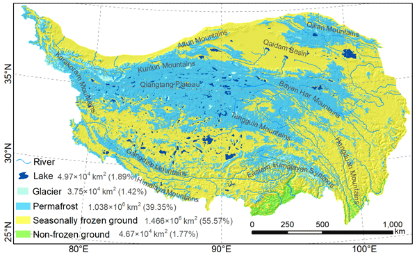
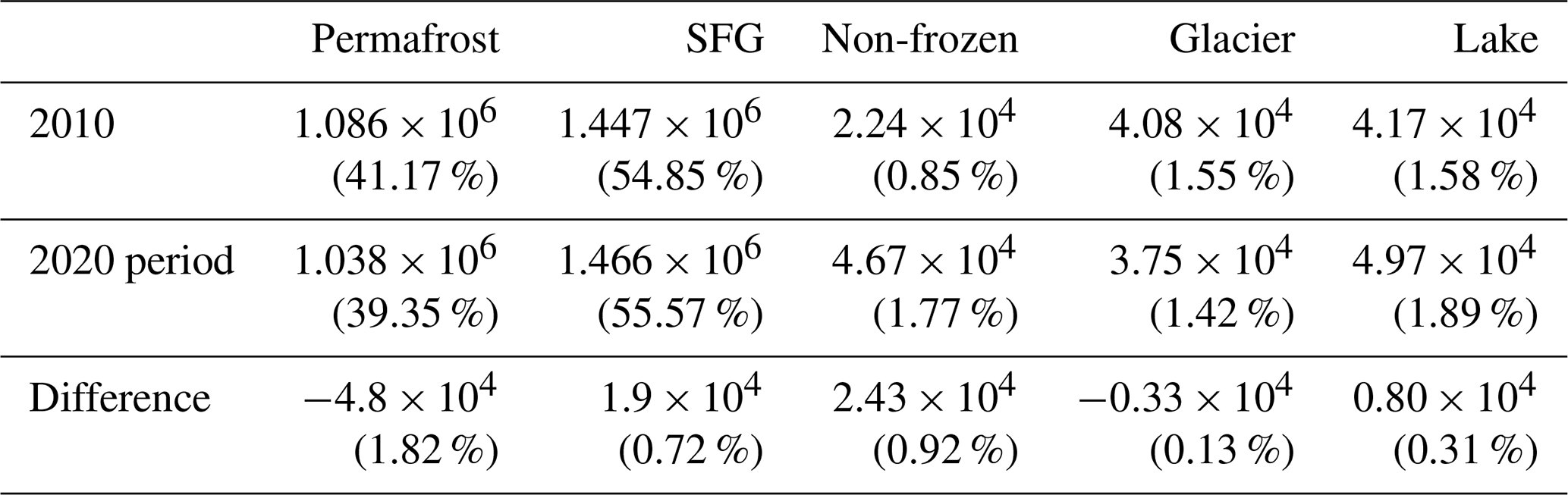
The final 2020-period permafrost distribution map, generated using the optimized RF-derived E parameter and corrected thermal forcing indices, is presented in Fig. 5. Statistical analysis shows that permafrost covers approximately 1.038 × 10⁶ km2, accounting for 39.35 % of the total QTP area (excluding lakes and glaciers). SFG is the dominant frozen ground type, occupying 1.466 × 10⁶ km2 (55.57 %), while non-frozen ground is confined to the lowest marginal valleys (4.67 × 10⁴ km2, 1.77 %).
The spatial pattern of the 2020-period map exhibits a strong altitudinal and latitudinal zonality, consistent with the region's topoclimatic gradients. The most extensive continuous permafrost body is concentrated in the high-elevation interior, encompassing the Qiangtang Plateau, the Hoh Xil region, and the Bayan Har Mountains. The combination of extreme elevation (> 4500 m) and an arid, continental climate maintains a stable, negative ground thermal regime. This continuous zone forms the cold core of the plateau, interrupted only by large endorheic lakes, which form localized taliks. To the north, the Qaidam Basin creates a distinct break in the permafrost continuity. Despite its high latitude, the basin's much lower elevation and distinctive arid-desert thermal regime preclude permafrost formation, creating a vast expanse of SFG that physically isolates the permafrost of the Qilian Mountains from the main plateau body.
Moving southward and eastward from the Qiangtang core, permafrost becomes increasingly fragmented. In the eastern QTP, particularly in the Three-River Headwater Region, the landscape is dominated by SFG, with permafrost confined to high ridges. This pattern is likely shaped by the advective heat transport from the developed river networks and by the relatively lower latitude, rendering permafrost in this region thermally fragile (Zhang et al., 2022). Similarly, along the southern and southeastern margins (the Himalayas, the Gangdise Mountains, and the Hengduan Mountains), permafrost distribution is strictly topographically controlled. Here, the combination of lower latitude and deeply dissected terrain creates sharp thermal gradients. Permafrost occurs discontinuously, clinging to high-altitude ridgelines and islands of extreme elevation, while the deep, incised valleys remain non-frozen ground or SFG.
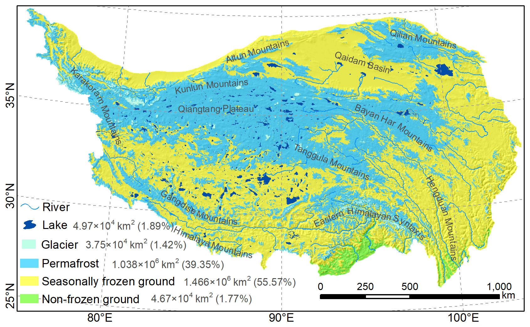
Figure 5Map of frozen ground distribution at 1 km resolution over the QTP in the 2020 period. Areas and percentages of frozen soil types are present. Glacier extent data are derived from Ye et al. (2017), and the 2020 lake boundaries are obtained from Zhang et al. (2021).
4.4 Accuracy assessment and inter-comparison
4.4.1 Validation against borehole observations and uncertainty analysis
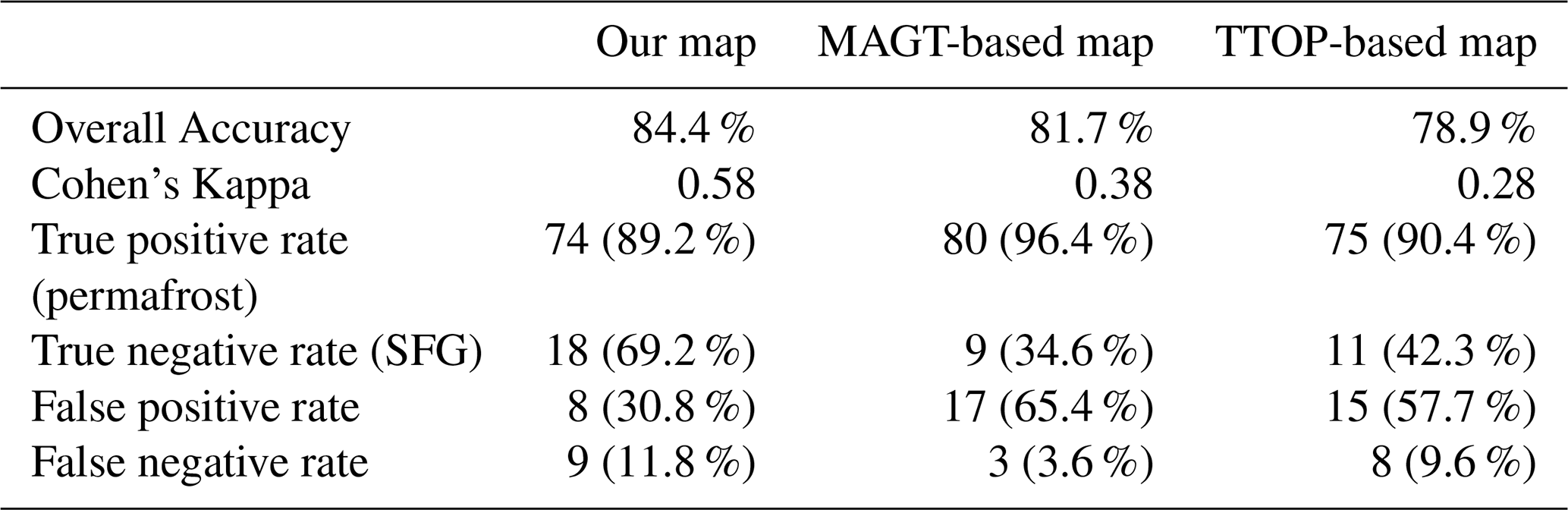
Quantitative validation was performed using 109 independent borehole records from the 2020 period (Table 2). Our map achieved an overall accuracy of 84.4 % and a Cohen's Kappa coefficient of 0.58, outperforming both the MAGT-based map (81.7 %, κ=0.38) and the TTOP-based map (78.9 %, κ=0.28).
A key advantage of our approach lies in its balanced classification capability. While both reference maps showed high sensitivity, identifying over 90 % of confirmed permafrost sites, they suffered from significant commission errors, frequently misclassifying SFG as permafrost. In contrast, our map differentiated SFG far more effectively, achieving a true negative rate of 69.2 %, compared with just 34.6 % for the MAGT-based map and 42.3 % for the TTOP-based map. This improvement indicates that our method effectively mitigates the overestimation of permafrost extent common in existing simulations. Furthermore, the multi-member ensemble simulations demonstrates that the uncertainty in the predicted soil parameter E has a limited impact on the final permafrost classification (detailed in Appendix C). The 16 ensemble-derived permafrost maps show high spatial and areal consistency, with the estimated total permafrost area varying within a narrow range, from 1.036 × 10⁶ to 1.043 × 10⁶ km2. This robustness is further substantiated by the permafrost agreement probability, where highly stable pixels (Pagree≥0.8) account for 98.85 % of the entire plateau, leaving 1.15 % of the region within the zone of classification inconsistency (where the 16 ensemble members disagree).
Table 1Comparison of the predictive accuracy of four sampling strategies for estimating the local soil parameter E for 2010. The baseline parameter E used for validation was derived from Cao et al. (2023). Accuracy metrics (RMSE, MAE, r, and % variance explained) are derived from 5-fold cross-validation using an optimal sample size of 5000 points.
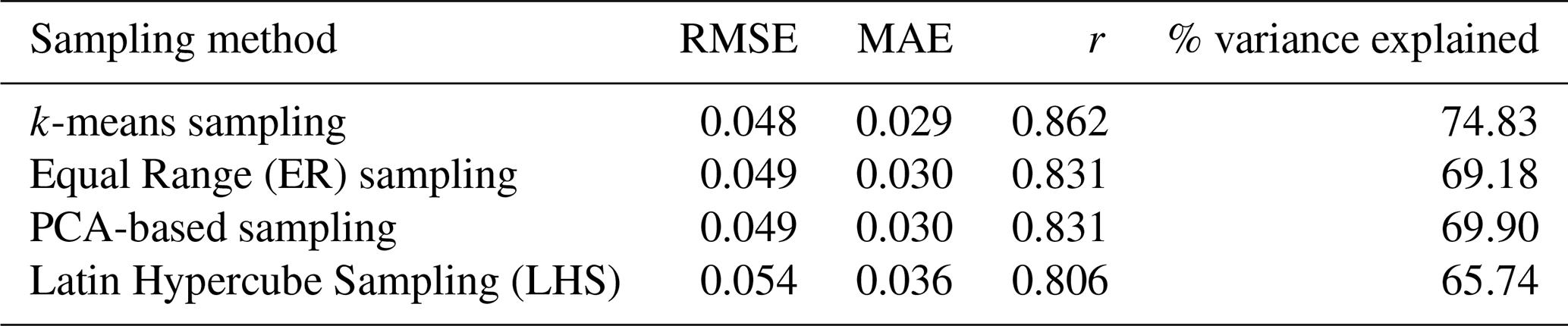
Table 2Confusion matrix describing the performance of the evaluated permafrost maps (Our map, MAGT-based map, Zou et al., 2025, and TTOP-based map, Yan et al., 2023) against 109 borehole validation sites. MAGT: mean annual ground temperature; TTOP: temperature at the top of permafrost.
4.4.2 Spatial inter-comparison
To further test the map's physical realism, we analyzed spatial inconsistencies between our results and the reference maps in several subregions (Fig. 6), specifically focusing on transition zones where modelling uncertainty is typically high. Notable discrepancies emerged in these areas, where ground observations consistently favored our simulation over the reference datasets.
In the Gaize area (subregion A in Fig. 6a, b) both reference maps failed to identify the seasonally frozen status of borehole ZK043 (Figs. 7a, 8a), whereas our map correctly classified it as SFG. Additionally, our map correctly identified borehole ZK042 as SFG, a site also situated in this transition zone. In the northern marginal zone between the Altun and Kunlun Mountains (subregion B in Fig. 6a), ground observations indicate the presence of four SFG boreholes (Fig. 7b). Our map correctly recognized all four, whereas the MAGT-based map identified only one (Fig. 7b). Although our simulation classified two confirmed permafrost boreholes in this region as SFG (Fig. 7b), observational records indicate these sites possessed extremely warm MAGT of −0.13 °C in 2013–2016 and −0.17 °C in 2013–2018. Such values are characteristic of thermally unstable permafrost that is highly susceptible to degradation, suggesting that our map likely captures a recent transition to SFG that predates the borehole's historical baseline.
Further discrepancies were found in the headwaters of the Yangtze River (subregion C in Fig. 6a, b). Here, our map correctly identified four out of five confirmed SFG boreholes, whereas the MAGT-based map identified only one (Fig. 7c) and the TTOP-based map identified three (Fig. 8b). While our simulation misclassified three confirmed permafrost boreholes in this region as SFG (Fig. 7c), it is important to note that these sites are situated within a permafrost transition zone where MAGTs range from −0.37 to −0.48 °C. These close to zero values suggest that the classification discrepancy may reflect real-world degradation or the inherent uncertainty in modeling such marginal thermal states. Crucially, meteorological station 56004 in this area was classified as permafrost by both reference maps but as SFG by ours (Figs. 7c, 8b). Analysis of in-situ GST (0 cm) data (2016–2019) at this site revealed a thawing index (DDT ≈ 2004 °C ⋅ d) significantly exceeding the freezing index (DDF ≈ 1332 °C ⋅ d). Because a thawing index that exceeds the freezing index is robust indicator of SFG, this observation provides strong evidence that our simulation offers a more reliable representation of the current thermal regime.
In the headwaters of the Yellow River (subregion D in Fig. 6a), the SFG borehole XXH-1 was correctly classified by our map but was misclassified as permafrost by the MAGT-based map (Fig. 7d). Notable spatial inconsistencies were also observed along the southern margin of the plateau (subregion E in Fig. 6b), but this area was excluded from the detailed inter-comparison due to the lack of available borehole observations for validation.
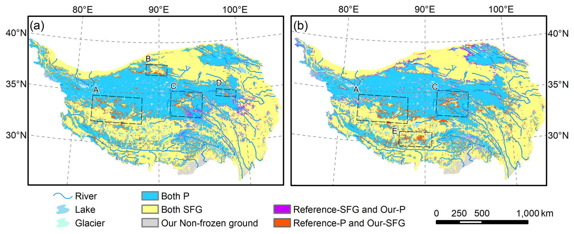
Figure 6Spatial inconsistencies in the distribution of frozen ground between the generated 2020-period permafrost map and reference datasets: (a) the MAGT-based map (Zou et al., 2025) and (b) the TTOP-based map (Yan et al., 2023). “Both P” (blue) and “Both SFG” (yellow) denote consistent classification. “Reference-P and Our-SFG” represents regions classified as permafrost by the reference map but as SFG in our map. “Reference-SFG and Our-P” indicate the opposite. The dashed boxes mark specific transition zones with obvious inconsistency: (A) Gaize and its vicinity, (B) the Altun–Kunlun Mountains transition zone, (C) the headwaters of the Yangtze River, (D) the headwaters of the Yellow Rive, and (E) the southern margin.
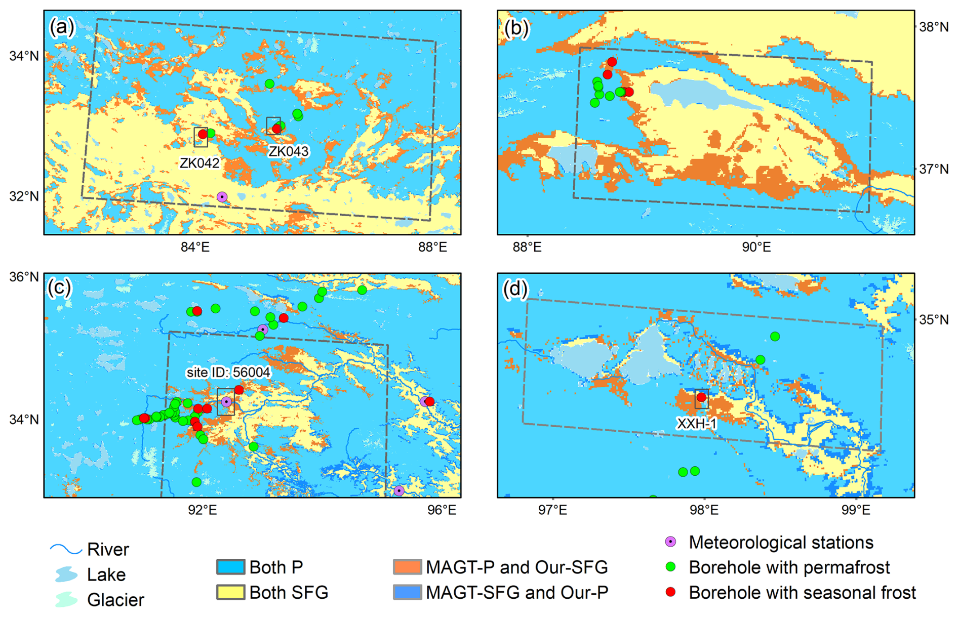
Figure 7Detailed validation of spatial inconsistencies between the generated 2020 map and the MAGT-based map using ground-truth observations. The panels (a)–(d) correspond to the four subregions (A–D) outlined in Fig. 6a.
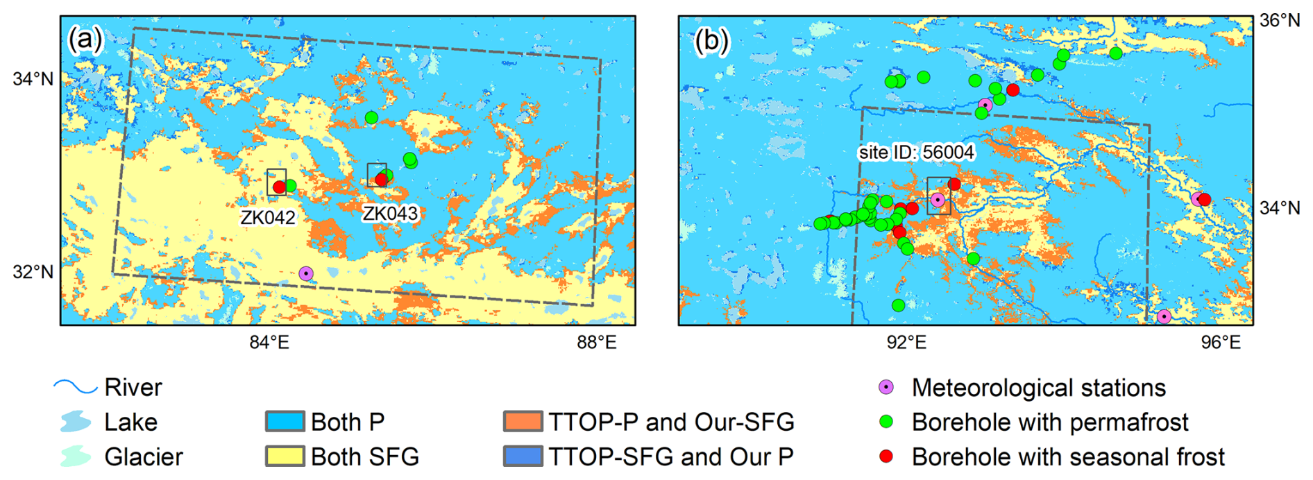
Figure 8Detailed validation of spatial inconsistencies between the generated 2020 map and the TTOP-based map in two key transition zones. The panels (a) and (b) correspond to the subregions (A and C) outlined in Fig. 6b.
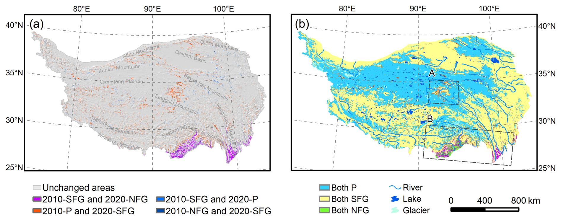
Figure 9Spatiotemporal evolution of frozen ground types on the QTP from the 2010 to 2020 period. (a) The spatial distribution of transition types overlaid on a hillshade map. (b) The same transitions shown against the background of the 2010-period permafrost distribution. The rectangles delineate two hotspots of significant change: subregion A (central QTP) and subregion B (southern QTP).
4.5 Decadal changes in frozen ground distribution (2010–2020 period)
Between the 2010 and 2020 periods, frozen ground distribution on the QTP underwent a distinct phase of degradation (Fig. 9), characterized by a net loss of permafrost extent and a concurrent expansion of SFG and non-frozen ground (Fig. 9a). Spatially, these shifts were not uniform but exhibited a clear bifurcation between the plateau's interior and its margins. Quantitative analysis indicates that the total permafrost area decreased by approximately 4.8 × 10⁴ km2 over the decade, representing a decline of 1.82 % relative to the total area (Table 3). This loss was primarily driven by the conversion of unstable permafrost into SFG. Consequently, the SFG area expanded by 1.9 × 10⁴ km2 (a 0.72 % increase). More strikingly, non-frozen ground area increased by 2.43 × 10⁴ km2 (a 0.92 % increase), reflecting a marked contraction of the frozen ground domain at its lower elevational and latitudinal limits.
These transitions reveal two dominant degradation patterns of degradation. In the central QTP region (subregion A in Fig. 9b), degradation of permafrost into SFG occurred extensively at the permafrost-SFG transition zones. This process accounted for 7.41 % of the total changed area and was largely concentrated in the transitional zones of the Qiangtang Plateau. In contrast, the southern and southeastern margins (subregion B in Fig. 9b), particularly the flanks of the Hengduan, Himalayan, and Gangdise mountains, experienced marginal retreat. The dominant transition was the conversion of SFG to non-frozen ground, which accounted for 39.62 % of the total changed area (Fig. 9b). This shift indicates a vertical ascent of the frozen ground lower limit in response to warming.
Beyond the ground thermal state itself, surface hydrological and glaciological features also responded to the warming climate. During this period, the glacier area decreased by 0.33 × 10⁴ km2 (Ye et al., 2017), while the lake area expanded by 0.80 × 10⁴ km2 (Zhang et al., 2021) (Table 3), consistent with the broader warm-wet climate trend observed across the region.
Table 3Areas and decadal changes for different frozen ground types, glaciers, and lakes on the QTP from the 2010 to 2020 period. Absolute areas are provided in km2, with percentages of the total areas shown in parentheses.
5.1 Mechanisms driving changes in soil parameter E variation and permafrost degradation
The decadal changes in E offer useful insight into the factors controlling permafrost stability on the QTP. Although the plateau experienced a general wetting trend during the study period (Zhang et al., 2021), regions with increasing E received substantially smaller precipitation increases (median +1.28 mm) than regions with decreasing E (median +2.23 mm) (Fig. 10). Because high-resolution soil moisture products are not available for the QTP, mean annual precipitation is used here as a proxy for regional soil moisture conditions. The effect size for precipitation (Cohen's d=0.020) was notably larger than those for NDVI and FSC (Cohen's d=0.010 and 0.005, respectively). These results suggest that spatial differences in soil moisture, as indicated by precipitation, play a larger role than vegetation or snow cover in modulating ground thermal conditions.
Soil moisture exerts strong control over the ground thermal regime because of its high specific heat capacity and latent heat of fusion. In areas where precipitation increased only modestly, soils likely remained relatively drier. Drier soils have lower thermal inertia and are therefore more responsive to atmospheric warming, which enhances ground heat uptake and drives an increase in E. In contrast, areas with greater precipitation increases likely maintained higher soil moisture levels, which increased thermal inertia and buffered the ground against warming, resulting in a decline in E. This indicates that even under a general warm-wet climate trend, spatial heterogeneity in soil moisture can drive divergent permafrost trajectories across the plateau.
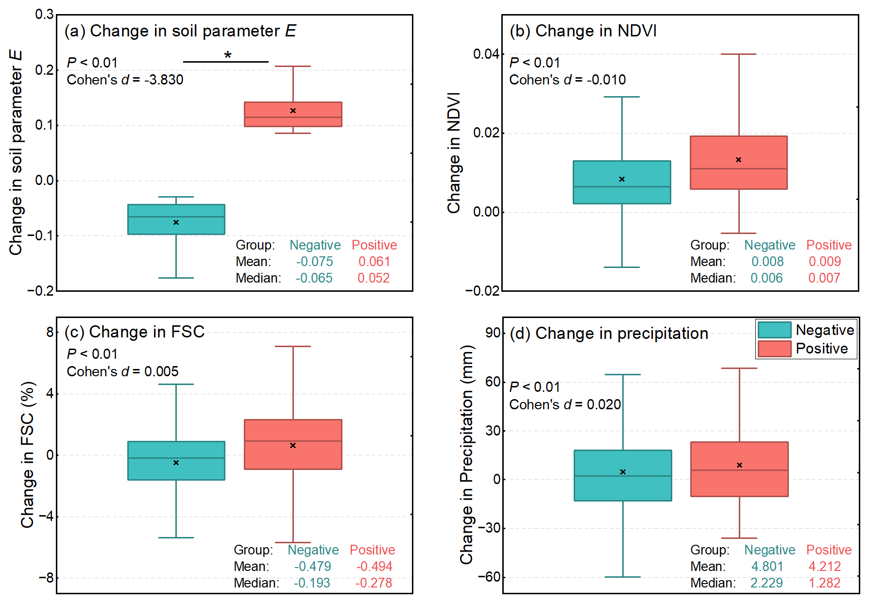
Figure 10Distribution of decadal changes (2010–2020) in key environmental factors, categorized by the trend in soil parameter E. Boxplots compare changes in (a) soil parameter E, (b) NDVI, (c) FSC, and (d) precipitation between regions of increased degradation potential (positive group) and reduced degradation potential (negative group). In each box plot, the centre line shows the median, the box represents the lower and upper quartiles (25th–75th percentiles), and the whiskers extend to the furthest data points within 1.5 times the interquartile range. The “x” marks the mean. Asterisks indicate significant differences between the two groups (Welch Two Sample t-test, P<0.01 and |Cohen's ).
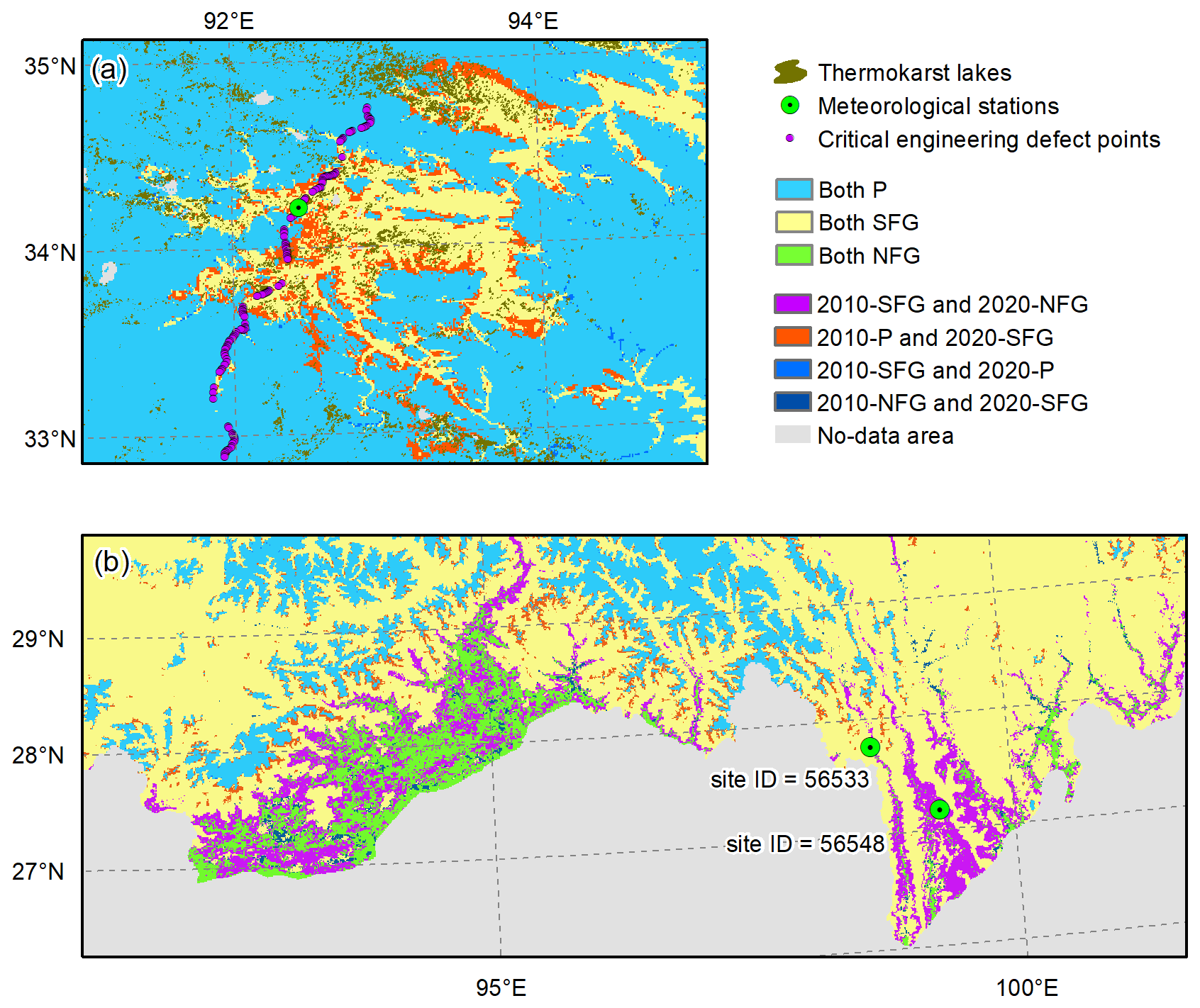
Figure 11Distribution and changes of frozen ground types in two degradation hotspots on the QTP from 2010 to 2020 periods. Panels (a) and (b) corresponds to subregions A and B in Fig. 9, respectively. (a) Changes in the central QTP, where the dominant transition is from permafrost to SFG. Thermokarst lakes (extracted from Sentinel-2A imagery) (Chen et al., 2021) and engineering defect points (mapped via manual field surveys) (Li, 2021) are superimposed on the map to serve as proxies for permafrost instability. (b) Changes in the southern QTP, characterized by the transition from SFG to non-frozen ground. The observed 0cm GST values from two meteorological stations (ID: 56533, 56548) provide validation for the model results.
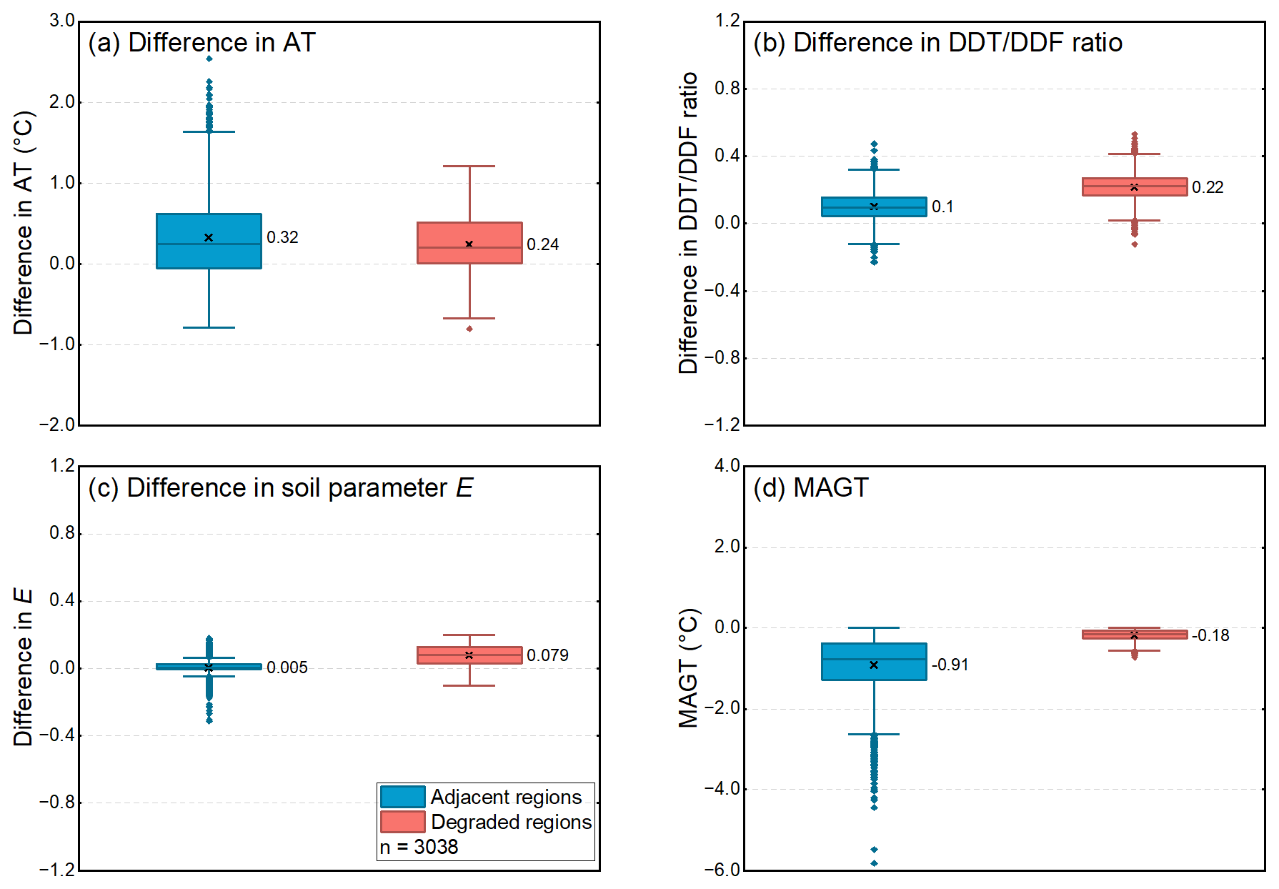
Figure 12Comparison of key environmental variables between degraded regions (permafrost to SFG) and adjacent stable permafrost regions in subregion A of Fig. 9b (Central QTP). The boxplots compare decadal changes (2010–2020) in (a) air temperature (AT), (b) the DDT DDF ratio, and (c) the soil parameter E. Positive values indicate an increase over the decade. Panel (d) compares the MAGT in 2010–2019. In each box plot, the center line shows the median, the “x” marks the mean, the box represents the lower and upper quartiles (25th–75th percentiles), and the whiskers extend to the furthest data points within 1.5 times the interquartile range. Data points beyond the whiskers are plotted individually as outliers.
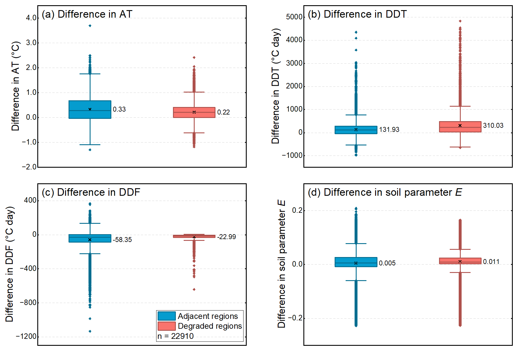
Figure 13Comparison of key environmental variables between degraded regions (SFG to non-frozen ground) and adjacent SFG regions in subregion B of Fig. 9b (Southern QTP). The panels compare decadal changes in (a) air temperature (AT), (b) DDT, (c) DDF, and (d) the soil parameter E. Positive values indicate an increase over the decade. In each box plot, the centre line shows the median, the “x” marks the mean, the box represents the lower and upper quartiles (25th–75th percentiles), and whiskers extend to the furthest data points within 1.5 times the interquartile range. Data points beyond the whiskers are plotted individually as outliers.
The spatial pattern of permafrost degradation lends further support to this interpretation. As shown in Fig. 11a, the dominant transition in the central QTP was from permafrost to SFG, concentrated in the transition zone between the two frozen ground types. This region is characterized by relatively warm permafrost, which is particularly sensitive to thermal perturbations (Zhang et al., 2022). The close spatial correspondence between simulated degradation areas and the distribution of thermokarst lakes identified from Sentinel-2A imagery (Chen et al., 2021) and known engineering defect points (Li, 2021) provides independent evidence that the observed changes reflect real physical instability.
A closer comparison of degraded and adjacent stable permafrost regions (Fig. 12) shows that air temperature changes alone cannot explain the divergence. While both regions experienced similar atmospheric warming (mean increase of 0.24 °C in degraded areas versus 0.32 °C in stable areas), the ground thermal response differed significantly (Fig. 12a). The ratio of thawing to freezing indices (DDT DDF) increased by 0.22 in the degraded zones, more than double the increase observed in the stable zones (0.10) (Fig. 12b). This amplified thermal forcing, combined with the significant rise in E (+0.079 versus +0.005), appears to have pushed already marginal permafrost (with MAGT close to 0 °C, Fig. 12d) across the thaw threshold.
In the southern QTP, the primary process was the conversion of SFG to non-frozen ground (Fig. 11b). This transition was accompanied by a much larger increase in the thawing index in degraded areas (310.03 °C ⋅ d) than in adjacent stable SFG regions (131.93 °C ⋅ d), while changes in the freezing index were minimal (Fig. 13). The marked increase in E (Fig. 13d) in degraded southern regions suggests that land-surface feedbacks further accelerated the loss of seasonal frost. These contrasting patterns indicate that the dominant mechanisms differ between the central and southern parts of the plateau.
5.2 Practical implications of the new permafrost map
The 2020-period permafrost distribution map produced here offers real practical value for engineering risk assessment and environmental management on the QTP. The spatial pattern of permafrost degradation corresponds closely with known locations of engineering defects along the Qinghai-Tibet Railway and Highway. This alignment suggests that the map successfully captures areas of subsurface thermal instability that contribute to infrastructure damage, making it a useful tool for identifying high-risk zones that may need enhanced monitoring or reinforced engineering measures.
Beyond its engineering applications, the map provides important information for assessing the resilience of the Asian Water Tower. Changes in permafrost and SFG conditions directly affect soil hydrology, groundwater flow, and vegetation dynamics across the headwater regions of major Asian rivers. By offering a temporally specific snapshot of frozen ground conditions rather than a long-term climatological average, this dataset enables a more accurate evaluation of how recent climate change has altered hydrological processes in these critical source areas.
Beyond these applications, the map also fills a key data gap in cryospheric research. Most existing permafrost maps of the QTP are based on multi-decadal averages and so do not reflect the current thermal state of the ground. The 2020-period map provides a temporally constrained benchmark that can support more rigorous calibration and validation of hydrological, ecological, and land surface models. This is especially valuable for studies that require year-specific or period-specific boundary conditions to simulate recent environmental changes or to project future permafrost evolution under different climate scenarios.
5.3 Model robustness and transferability of the mapping approach
The comparative evaluation of transfer learning strategies showed that the RF regression approach, combined with representative spatial sampling, provided robust and physically plausible estimates of E across the QTP. In contrast, the MLP approach achieved high accuracy within the training subregions but overfit severely and generated unrealistic spatial patterns when applied plateau-wide. This highlights a common challenge in applying deep learning models to large, heterogeneous regions: without strong physical constraints, such models can fit local patterns in the training data yet fail to generalize across diverse environmental conditions. The superior performance of the RF-based method here likely reflects its ability to capture complex, non-linear relationships while remaining relatively robust to noise and outliers. By treating the estimation of E as a regression problem against a spatially continuous 2010 field, rather than relying solely on sparse field survey data, the approach benefited from greater spatial coverage and reduced sampling bias. The use of k-means clustering sampling further improved model performance by ensuring that training samples represented the full range of environmental conditions across the plateau.
Despite its robustness on the QTP, the mapping framework has several limitations that constrain its transferability to other permafrost regions. The space-for-time substitution strategy relies on the assumption that the statistical relationship between E and environmental drivers remains approximately stationary over the extrapolation period. This assumption is more likely to hold in relatively stable alpine environments over decadal timescales, but may break down under rapid or non-linear environmental changes, such as widespread thermokarst development or large-scale land-use change.
Applying the framework successfully to other regions would also require local recalibration of E. The statistical relationships derived for the QTP cannot be transferred directly, since E reflects region-specific interactions among climate, soil properties, vegetation, and topography. High-quality field survey data from the target region would therefore be needed to establish a new benchmark E field there. The correction applied to satellite-derived thawing indices would also need to be adapted to local conditions. The multiple linear regression model used here was optimized for the QTP, where winter snow cover is generally thin and ephemeral. In regions with thick, persistent snow cover, such as much of the Arctic or boreal Canada, an explicit snow insulation term would be needed when calculating the freezing index. Overall, while the core components of the methodology, including the extended FROSTNUM framework, space-for-time substitution, and machine learning-based estimation of E, are conceptually transferable, applying them successful elsewhere depends on the availability of high-quality local calibration data and appropriate adaptation of the thermal-index correction procedures.
5.4 Limitations and future directions
Despite its overall robustness, the methodology presented in this study is subject to several limitations. First, the permafrost distribution map primarily reflects the thermal state of the shallow subsurface, typically at depths of around 10–15 m. It does not resolve deep or relict permafrost that may persist below the depth of zero annual amplitude. Consequently, areas classified as SFG in the 2020-period map may still contain permafrost at greater depths that has not yet fully responded to recent warming. Therefore, SFG areas identified in the map should be interpreted as regions where permafrost was not detected within the resolved depth range, rather than as areas where permafrost has completely disappeared.
Second, the space-for-time substitution strategy assumes that the relationship between E and its environmental drivers remains sufficiently stable over the study period. While this assumption appears reasonable over decadal timescales on the QTP, it may introduce greater uncertainty when the method is applied over longer time periods or in areas undergoing rapid environmental disturbances. As discussed in Sect. 5.3, this limitation also constrains the direct transferability of the current framework to other permafrost regions without local recalibration.
Third, due to the lack of updated large-scale field surveys across the QTP, the E parameter for the 2020 period remains a modeled estimate rather than a directly calibrated observation. Although cross-validation and ensemble analysis support the robustness of these predictions, new field data would still be valuable for further constraining spatial variability under current conditions.
These limitations point to several priorities for future research. Collecting new, spatially representative field data across the QTP would strengthen the calibration of E. In addition, developing physics-constrained machine learning models and integrating the current empirical approach with process-based simulations could help address non-stationarity and better represent abrupt permafrost changes.
This study produced a 1 km resolution permafrost distribution map of the QTP for the 2020 period by advancing the FROSTNUM framework. To address the challenge of data scarcity in updating the map, we used a space-for-time substitution strategy to estimate the critical soil parameter E. Our comparative evaluation showed that the RF regression approach, trained on representative spatial samples from the 2010 map, provided robust and physically realistic estimates of E. The unconstrained neural network (MLP) approach, in contrast, suffered from overfitting and produced unrealistic spatial artifacts.
The resulting 2020-period map shows that permafrost covers approximately 1.038 × 10⁶ km2 (39.35 % of the total QTP area), while SFG covers 1.466 × 10⁶ km2 (55.57 %). Validation against 109 independent borehole records yielded an overall accuracy of 0.84 and a Cohen's Kappa of 0.58, outperforming existing MAGT-based and TTOP-based products.
A systematic comparison with the 2010 baseline indicates substantial degradation of frozen ground over the decade. The total permafrost area decreased by 4.8 × 10⁴ km2 (a 1.82 % decrease), mainly through transition to SFG. Spatially, this degradation was concentrated in two distinct hotspots. In the central QTP, widespread degradation of unstable permafrost accounted for 7.41 % of the total change. In contrast, the southern margins experienced a rapid contraction of the frozen ground domain, where conversion of SFG to non-frozen ground accounted for 39.62 % of the total changes.
This study provides an up-to-date, high-resolution permafrost distribution map of the QTP. The map offers a temporally specific reference to support engineering risk assessment, ecological monitoring, and the calibration of land surface models in this rapidly warming region.
We implemented a representative sampling framework to train the RF model efficiently while capturing the full heterogeneity of the QTP. The primary objective was to select a subset of training pixels from the full dataset (exceeding 2 million grid cells) that minimized information redundancy while maximizing the environmental variance covered by the model. This is important for reducing predictive uncertainty, particularly for rare but physically significant permafrost conditions. We evaluated four distinct sampling algorithms: k-means clustering sampling (Brus et al., 2006), the Equal Range (ER) sampling (Hengl et al., 2003), Principal Component Analysis (PCA)-based sampling (Hengl et al., 2003), and Latin Hypercube Sampling (LHS) (Carré et al., 2007) across four sample sizes (1000, 3000, 5000, and 10 000 points).
k-means clustering sampling: This method utilizes unsupervised learning to partition the multivariate environmental space into distinct clusters, ensuring that the training set represents distinct physical conditions rather than oversampling spatially abundant but homogeneous areas (Hartigan, 1975). We applied k-means algorithm to the vectors of the environmental covariates (topography, soil, vegetation, etc.). The algorithm partitions the study domain into k clusters by minimizing within-cluster sum of squares. For each cluster, the pixel closest to the geometric centroids in feature space was selected as the representative training sample. This approach inherently favors environmental representativeness over spatial proximity.
ER sampling: Standard random sampling often produces a majority-class bias, where the model learns the characteristics of common conditions well but fails to predict rare extremes. To mitigate this, we employed ER sampling, which stratifies the sampling domain based on the distribution of key environmental gradients (Hengl et al., 2003). The core principle of ER is to divide the entire range of a predictor variable into several equal-width strata (or histogram slices). Samples are then allocated within these strata proportionally to the data density. For example, considering a variable with a normal distribution divided into 5 clusters across its standard statistical range (−3σ to +3σ), the stratification limits correspond to cumulative probabilities of 3.6 %, 27.4 %, 72.6 %, 96.4 %, and 100 %. The resulting sampling weights assigned to these strata are therefore 0.036, 0.238, 0.452, 0.238, and 0.036, respectively. This method remains robust even for skewed distributions, an advantage it retains over simple equal-frequency binning. In our implementation, we generated sample allocations for each environmental factor independently, dividing the total target sample size equally across factors. These individual sample sets were then aggregated into a combined training pool. Finally, we applied a deduplication step to remove any overlapping points. Testing confirmed that this deduplication reduced the final count only negligibly, thereby preserving the intended sample size.
PCA-based sampling: The environmental covariates that drive permafrost distribution often exhibit high multicollinearity. The PCA-based method (Hengl et al., 2003) address this by transforming the original, correlated predictors into a set of principle components. Sampling was then conducted in this reduced PC space to maximize the coverage of environmental variability. In our implementation, we first performed a PCA analysis on all environmental factors and retained the components that cumulatively explained 95 % of the total variance. The total sample size was then allocated to these selected PCs in proportion to the variance each explained. For example, given a target of 10 000 samples, if the first PC accounted for 64 % of the variance, 6400 sample points were allocated to it. Specific points were then selected by stratifying each retained PC using the ER method and randomly drawing the allocated number of samples from within those strata.
LHS sampling: LHS is a constrained Monte Carlo scheme widely recognized for its efficiency in sampling when no prior soil samples exist and only ancillary data are available (Carré et al., 2007). It is a stratified-random procedure designed to ensure the full range of every variable is sampled with uniform probability. The method works by dividing the cumulative distribution of each of the k environmental variables into n equiprobable intervals (where n is the target sample size). A single value is then randomly selected from each interval for every variable. These n values for each variable are finally randomly paired to create n unique, multivariate sample points. This process ensures that the marginal distribution of each variable is maximally stratified, so that the training set covers the entire multivariate feature space without the clustering or gaps common in simple random sampling.
We evaluated the validity of the E predicted by the MLP model. This evaluation focused on both the statistical distribution of the predicted values and the spatial realism of the resulting permafrost simulation.
As shown in Fig. B1, the MLP-predicted E values exhibit a highly irregular statistical distribution that deviates from physical expectations. Approximately 53 % of the total pixels fall within the range of 0–2.0 (Fig. B1a), with the highest frequency heavily skewed towards the 0–0.1 interval. Conversely, the remaining 47 % of the values are scattered across an unrealistically wide range of 2.0–350 (Fig. B1b). This extreme bifurcation suggests the model failed to learn the continuous physical properties of the soil, instead overfitting to the binary classification targets.
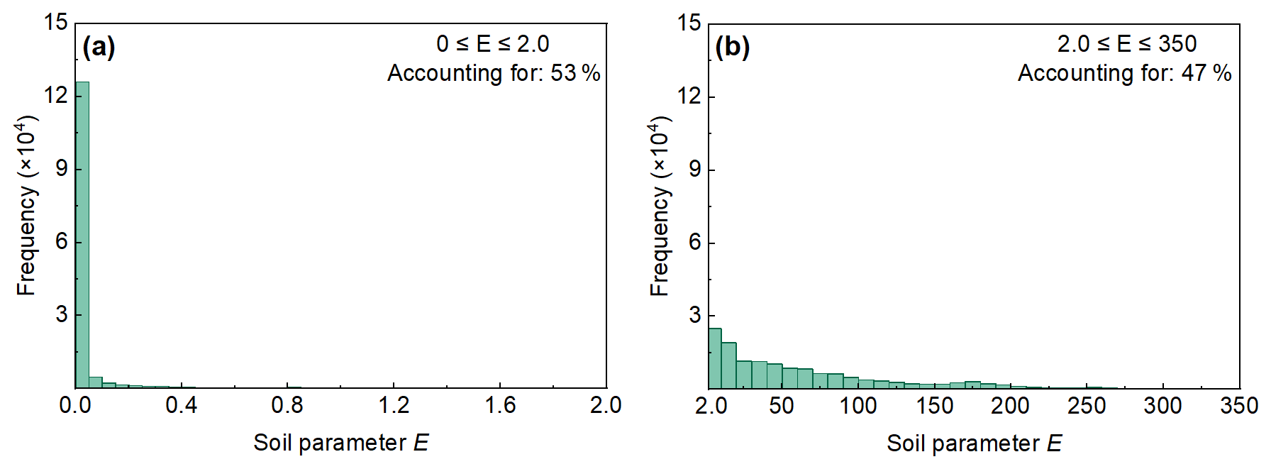
Figure B1Frequency histograms of the soil parameter E predicted by the MLP model. (a) Distribution of values within the range of 0 ≤ E ≤ 2.0, accounting for 53 % of total pixels. (b) Distribution of values within the range of 2.0 ≤ E ≤ 350, accounting for the remaining 47 %.
Spatially, the MLP-derived E field (Fig. B2a) displays significant inconsistencies when compared to the reference E distribution derived from the Particle Swarm Optimization algorithm with boundary constraints (Fig. B2b), which served as the validated baseline in Cao et al. (2023). Due to the absence of physical constraints, the MLP-derived E values exhibit extreme spatial heterogeneity and magnitude deviations of several orders.
The practical consequences of these artifacts become clear when the MLP-derived E field is used to reconstruct the 2010 permafrost distribution. The resulting map (Fig. B2c) exhibits a substantial visual and spatial mismatch with the rigorously validated 2010 baseline map (Fig. B2d). Given these fundamental discrepancies in both statistical distribution and spatial pattern, we conclude that the unconstrained MLP approach does not accurately reflect actual soil conditions. This method was therefore excluded from the final mapping workflow. Future applications of deep learning in this context would likely need physical constraints or penalty terms to ensure physically realistic parameter estimates.
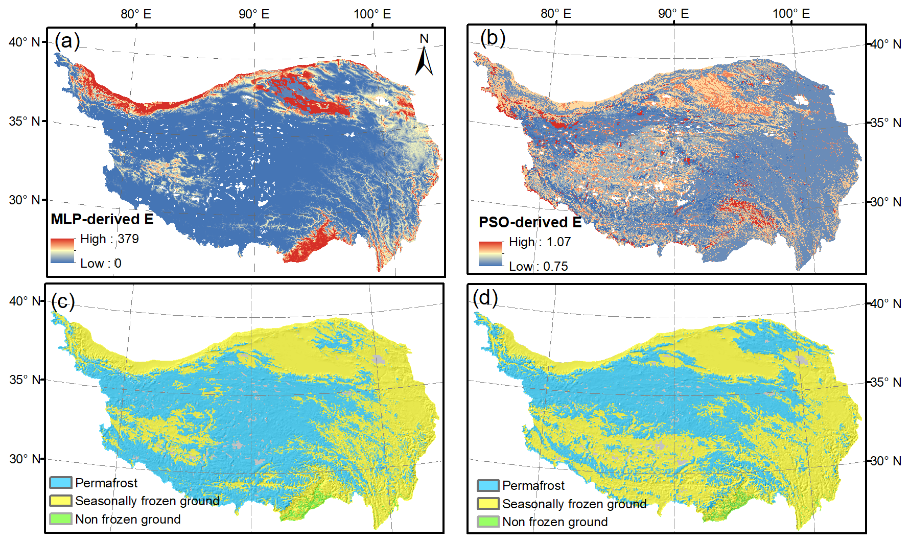
Figure B2Comparison of the spatial distribution of soil parameter E and the resulting frozen ground types. (a) Spatial distribution of E derived from the MLP model. (b) Spatial distribution of E derived from the Particle Swarm Optimization (PSO) algorithm (Cao et al., 2023). (c) Frozen ground distribution for 2010 simulated using the MLP-derived E. (d) Baseline frozen ground map for the year 2010 (Cao et al., 2023).
To assess the uncertainties associated with the choice of training sample selection, an uncertainty analysis was conducted for both the soil parameter E and the final permafrost map across the QTP. The analysis was based on 16 model configurations generated from combining four sampling strategies with four sample sizes.
The predicted soil parameter E shows a high degree of consistency among the 16 ensemble members (Fig. C1). The ensemble mean of E (Fig. C1a) exhibits a spatial pattern that is highly consistent with the E map derived from the optimal sampling scheme used in the main analysis (Fig. 4a). The standard deviation (SD) remains low across most regions of the plateau, generally below 0.04 (Fig. C1b). The coefficient of variance (CV) further demonstrates the stability of the predicted E values (Fig. C1c). Overall, 98.5 % of pixels have CV values below 5 %, with most pixels concentrated between 1.5 % and 2.5 % (Fig. C1d). Relatively higher CV values (5 %–7.5 %) are mainly found in the Qiangtang Plateau, where environmental conditions are more heterogeneous.
The uncertainty in the predicted soil parameter E has a limited influence on the final permafrost classification, resulting in a highly consistent permafrost map among the 16 ensemble simulation (Fig. C2). Spatially, the ensemble-derived permafrost maps show a high degree of consistency (Fig. C2a). Most areas are consistently classified as either permafrost or SFG across all 16 simulations. Areas with inconsistent classifications are limited and mainly occur along the boundaries between stable permafrost and SFG, where the classification is more sensitive to variations in the predicted E parameter.
The area estimates are also highly consistent among the 16 ensemble simulations (Fig. C2b). The total permafrost area ranges from 1.036 × 10⁶ to 1.043 × 10⁶ km2, while the SFG area ranges from 1.461 × 10⁶ to 1.468 × 10⁶ km2. The small spread among the ensemble members indicates that uncertainties in the predicted E parameter have a limited effect on regional-scale area estimates. This consistency is further confirmed by the distribution of permafrost agreement probability (Pagree, Fig. C2c). Stable SFG (Pagree ≤ 0.2) and stable permafrost (Pagree ≥ 0.8) account for 56.69 % and 42.16 % of the total pixels, respectively. In contrast, only 1.15 % of pixels fall within the transition zone (0.2 < Pagree < 0.8). The concentration of pixels near agreement probabilities of 0 and 1 indicates a high level of consistency among the ensemble members and demonstrates the robustness of the mapped permafrost distribution.
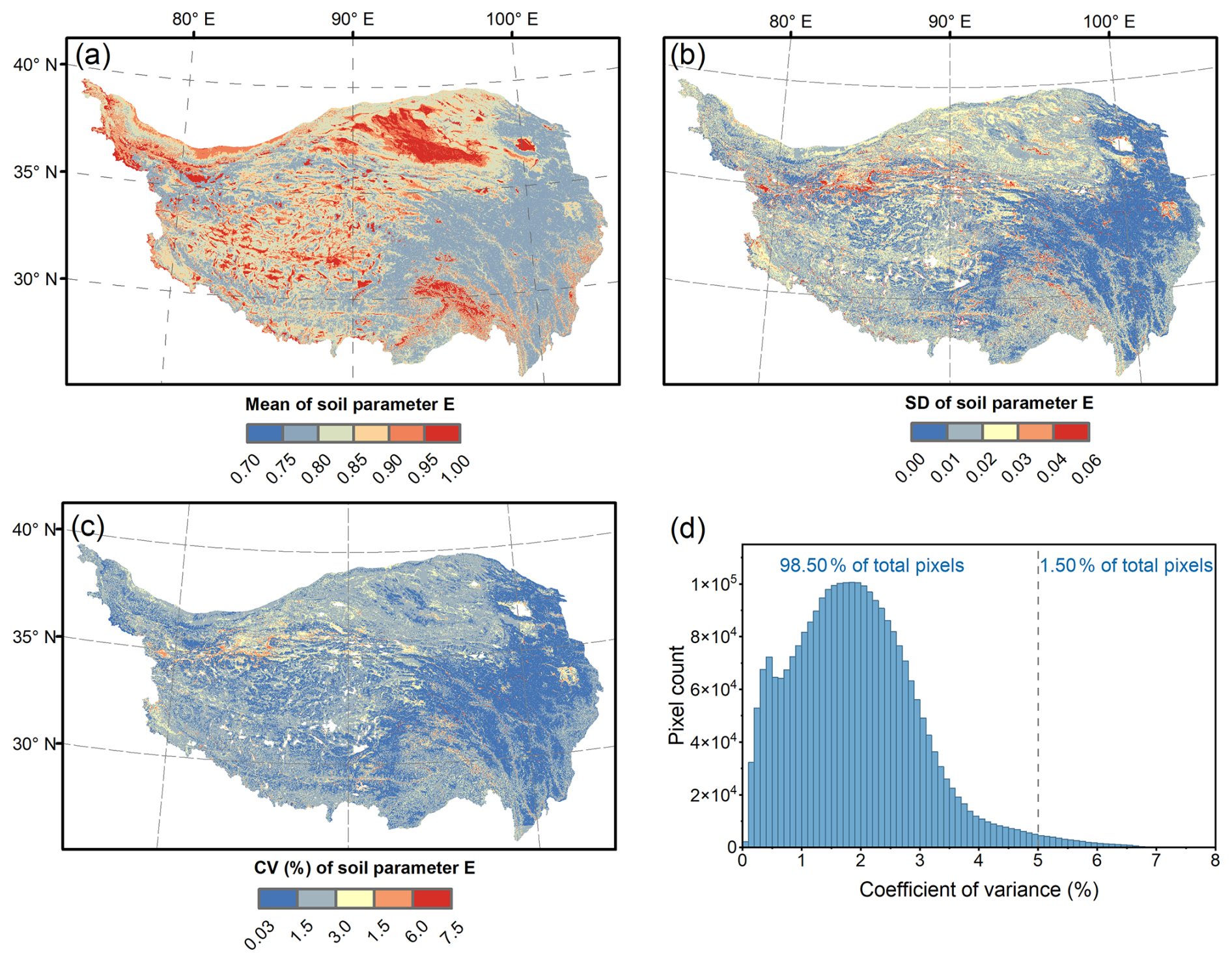
Figure C1Uncertainty assessment of the soil parameter E derived from 16 model configurations combining different sampling strategies and sample sizes. (a) Ensemble mean of E; (b) standard deviation (SD) of E; (c) coefficient of variance (CV, %) of E; and (d) frequency distribution of pixel-level CV values across the QTP. The dashed line in panel (d) indicates a CV threshold of 5 %, showing that 98.5 % of pixels exhibit CV values below this threshold. This ensemble quantifies uncertainty associated with the choice of sampling strategy and sample size. It does not capture other sources of uncertainty, such as errors in input datasets or potential non-stationarity of the driver–E relationship between 2010 and the 2020 period.
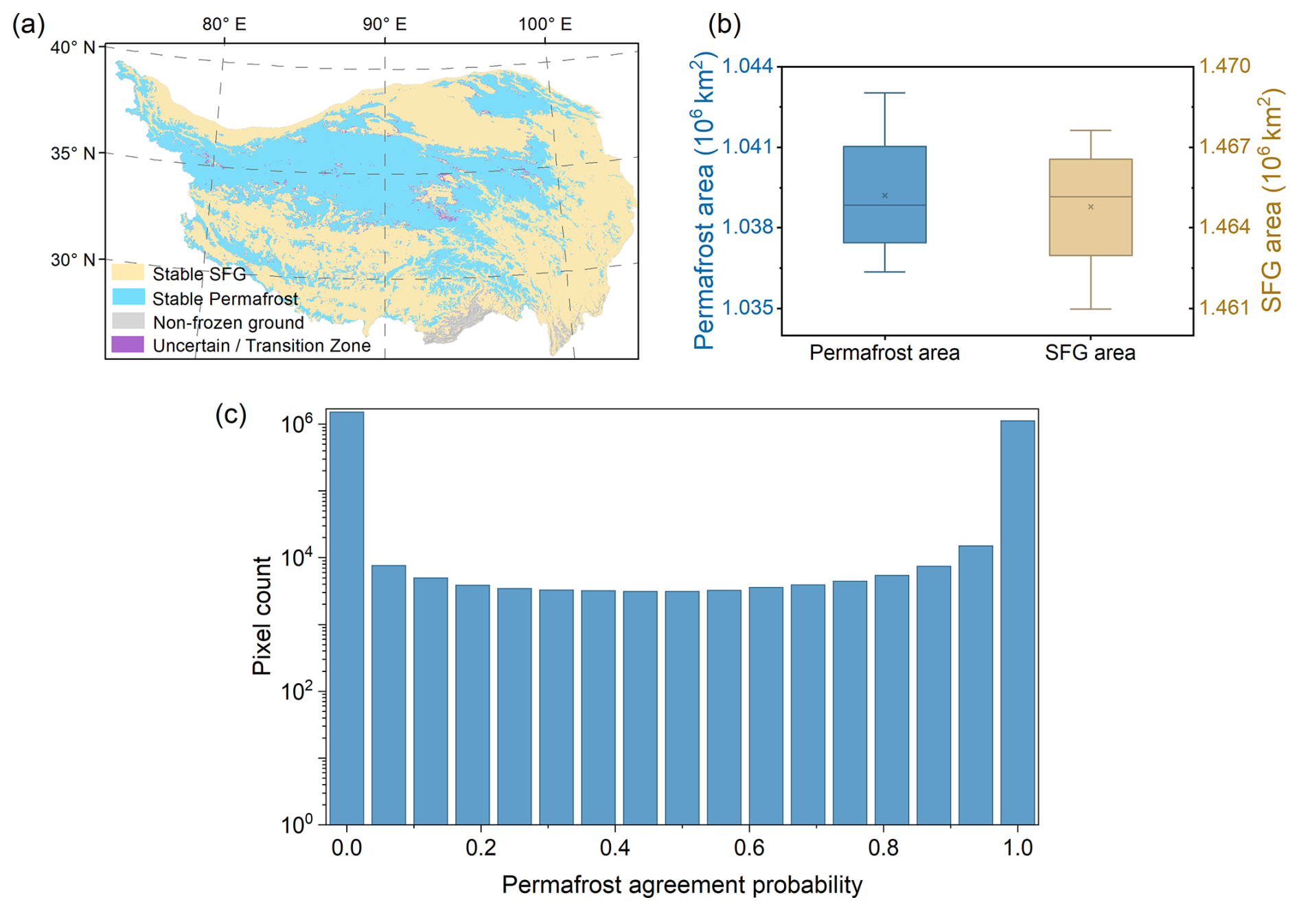
Figure C2Uncertainty assessment of simulated permafrost distributions derived from 16 parameter E maps. (a) Spatial classification consistency of the 16 ensemble members. Blue pixels indicate areas consistently classified as permafrost by all ensemble members (), yellow pixels indicate areas consistently classified as SFG, and purple pixels denote pixels with inconsistent classifications among ensemble members. (b) Uncertainty ranges of the total permafrost area (left axis) and SFG area (right axis) estimated from these ensemble members. (c) Frequency distribution of permafrost agreement probability (Pagree) across the QTP shown on a logarithmic scale (log10). Stable SFG (Pagree ≤ 0.2) and stable permafrost (Pagree ≥ 0.8) occupy 56.69 % and 42.16 % of the total pixels, respectively, whereas 1.15 % of pixels fall within the classification transition zone (0.2 < Pagree < 0.8). This analysis quantifies the robustness of the permafrost classification to variations in training sample selection. It does not represent the full uncertainty of the 2020-period permafrost map, as other important sources of uncertainty (e.g., input data errors and the space-for-time stationarity assumption) are not included in the ensemble.
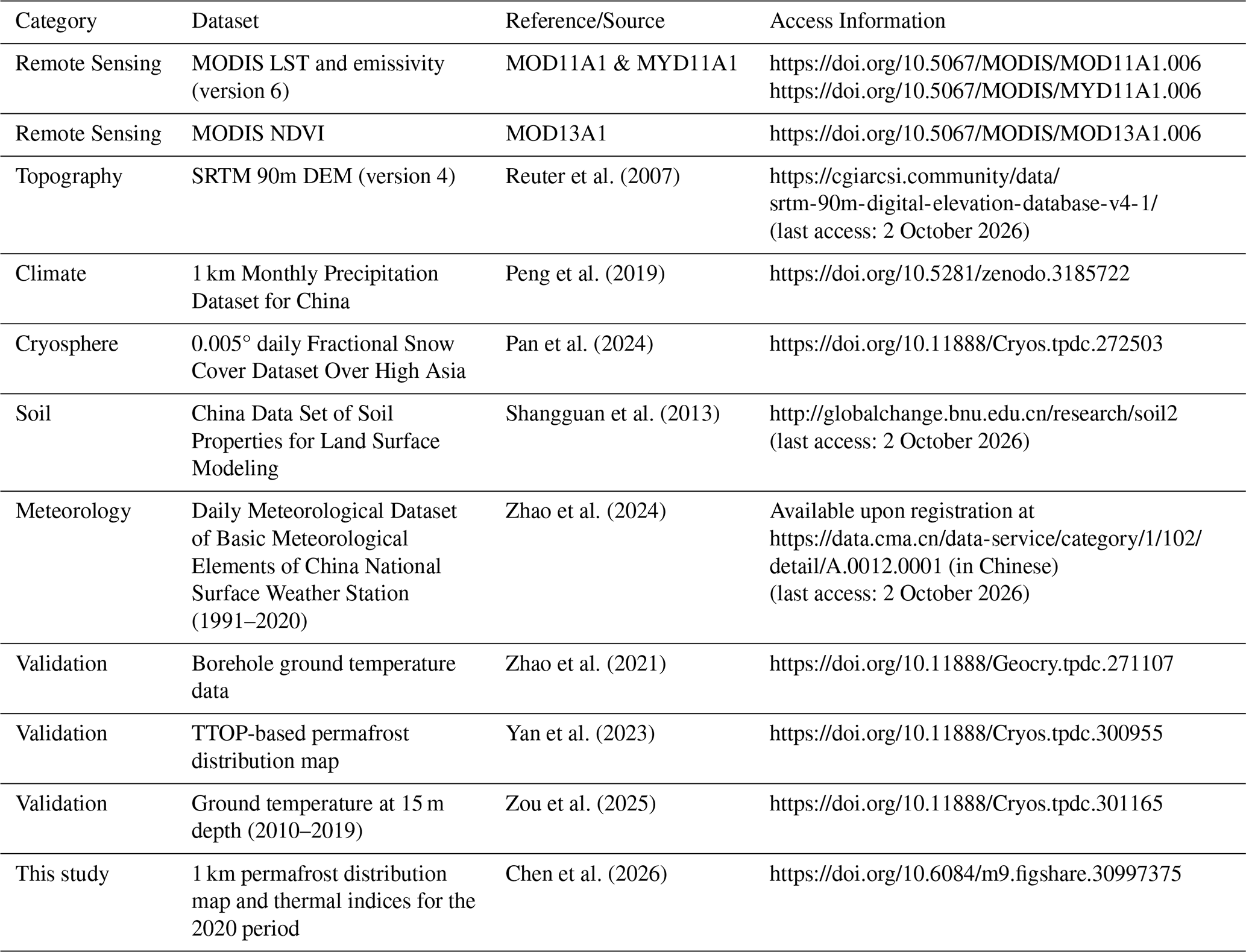
The 1 km resolution permafrost distribution of the QTP for the 2020 period and the associated annual ground surface thermal indices generated in this study are publicly available via Figshare at https://doi.org/10.6084/m9.figshare.30997375 (Chen et al., 2026). The resulting 2020 map is also archived at the National Cryosphere Desert Data Center at https://doi.org/10.12072/ncdc.permalab.db7813.2026 (Chen and Nan, 2026). The sources and access details for the third-party public datasets used for model forcing, environmental covariates, and validation are provided in Table D1.
Conceptualization, Z.N.; Methodology, Z.N. and Y.C.; Formal analysis, Y.C., W.T. and Y.Z.; Validation, Y.C. and Y.Z.; Writing – original draft, Y.C. and Z.N.; Writing – review and editing, Z.N., Y.C., S.Z., D.Y., G.J. and F.N.; Supervision, Z.N.; Funding acquisition, Z.N. and Y.C. All authors have read and agree to the published version of the manuscript.
The contact author has declared that none of the authors has any competing interests.
Publisher's note: Copernicus Publications remains neutral with regard to jurisdictional claims made in the text, published maps, institutional affiliations, or any other geographical representation in this paper. The authors bear the ultimate responsibility for providing appropriate place names. Views expressed in the text are those of the authors and do not necessarily reflect the views of the publisher.
The authors gratefully acknowledge the National Tibetan Plateau Data Center and NASA for providing the datasets used in this study. Sincere appreciation is also extended to the scientists who participated in the Second Tibetan Plateau Scientific Expedition and Research campaign for their dedicated efforts in collecting valuable in situ data across the Qinghai-Tibet Plateau.
This research was supported by the grant of National Natural Science Foundation of China (grant no. 42571149). Yuhong Chen was also supported by the Postdoctoral Research Funding of Hangzhou International Innovation Institute of Beihang University (grant no. 2025BKZ075).
This paper was edited by Anne Morgenstern and reviewed by two anonymous referees.
Brus, D. J., de Gruijter, J. J., and van Groenigen, J. W.: Designing spatial coverage samples using the k-means clustering algorithm, Chap. 14, in: Developments in Soil Science, edited by: Lagacherie, P., McBratney, A. B., and Voltz, M., Elsevier, Amsterdam, the Netherlands, 183–192, https://doi.org/10.1016/S0166-2481(06)31014-8, 2006.
Burke, E. J., Zhang, Y., and Krinner, G.: Evaluating permafrost physics in the Coupled Model Intercomparison Project 6 (CMIP6) models and their sensitivity to climate change, The Cryosphere, 14, 3155–3174, https://doi.org/10.5194/tc-14-3155-2020, 2020.
Cao, Z., Nan, Z., Hu, J., Chen, Y., and Zhang, Y.: A new 2010 permafrost distribution map over the Qinghai–Tibet Plateau based on subregion survey maps: a benchmark for regional permafrost modeling, Earth Syst. Sci. Data, 15, 3905–3930, https://doi.org/10.5194/essd-15-3905-2023, 2023.
Carré, F., Mcbratney, A. B., and Minasny, B.: Estimation and potential improvement of the quality of legacy soil samples for digital soil mapping, Geoderma, 141, 1–14, https://doi.org/10.1016/j.geoderma.2007.01.018, 2007.
Chadburn, S. E., Burke, E. J., Cox, P. M., Friedlingstein, P., Hugelius, G., and Westermann, S.: An observation-based constraint on permafrost loss as a function of global warming, Nat. Clim. Change, 7, 340–344, https://doi.org/10.1038/nclimate3262, 2017.
Chen, X., Mu, C., Jia, L., Li, Z., Fan, C., Mu, M., Peng, X., and Wu, X.: High-resolution dataset of thermokarst lakes on the Qinghai-Tibetan Plateau, Earth Syst. Sci. Data Discuss. [preprint], https://doi.org/10.5194/essd-2020-378, 2021.
Chen, Y. and Nan, Z.: A 2020 permafrost distribution map of the Qinghai-Tibet Plateau, National Cryosphere Desert Data Center [data set], https://doi.org/10.12072/ncdc.permalab.db7813.2026, 2026.
Chen, Y., Nan, Z., Cao, Z., Ou, M., and Feng, K.: A stepwise framework for interpolating land surface temperature under cloudy conditions based on the solar-cloud-satellite geometry, ISPRS – J. Photogramm. Remote Sens., 197, 292–308, https://doi.org/10.1016/j.isprsjprs.2023.02.004, 2023.
Chen, Y., Nan, Z., Tian, W., Zhao, Y., Zhao, S., Yang, D., Jing, G., and Niu, F.: A 2020 permafrost distribution map over the Qinghai-Tibet Plateau, Figshare [data set], https://doi.org/10.6084/m9.figshare.30997375, 2026.
Cheng, G., Li, S., and Nan, Z.: Map of permafrost on the Qinghai-Tibet Plateau (1:3 000 000) (1983–1996), National Tibetan Plateau Data Center [data set], https://doi.org/10.11888/Geocry.tpdc.270014, 1996.
Deng, H., Zhang, Z., and Wu, Y.: Accelerated permafrost degradation in thermokarst landforms in Qilian Mountains from 2007 to 2020 observed by SBAS-InSAR, Ecol. Indic., 159, 111724, https://doi.org/10.1016/j.ecolind.2024.111724, 2024.
Fu, Y., Horton, R., and Heitman, J.: Neural network estimation of thermal conductivity across full saturation for various soil types, Comput. Electron. Agric., 235, 110321, https://doi.org/10.1016/j.compag.2025.110321, 2025.
Gay, B. A., Pastick, N. J., Züfle, A. E., Armstrong, A. H., Miner, K. R., and Qu, J. J.: Investigating permafrost carbon dynamics in Alaska with artificial intelligence, Environ. Res. Lett., 18, 125001, https://doi.org/10.1088/1748-9326/ad0607, 2023.
Guo, D. and Wang, H.: Simulation of permafrost and seasonally frozen ground conditions on the Tibetan Plateau, 1981–2010, J. Geophys. Res.-Atmos., 118, 5216–5230, https://doi.org/10.1002/jgrd.50457, 2013.
Hachem, S., Allard, M., and Duguay, C.: Using the MODIS land surface temperature product for mapping permafrost: an application to northern Québec and Labrador, Canada, Permafrost Perigl., 20, 407–416, https://doi.org/10.1002/ppp.672, 2009.
Hartigan, J.: Clustering algorithms, Wiley, New York, USA, 364 pp., ISBN 0-471-35645-X, 1975.
Hengl, T., Rossiter, D. G., and Stein, A. G.: Soil sampling strategies for spatial prediction by correlation with auxiliary maps, Austr. J. Soil Res., 41, 1403–1422, https://doi.org/10.1071/SR03005, 2003.
Hjort, J., Streletskiy, D., Doré, G., Wu, Q., Bjella, K., and Luoto, M.: Impacts of permafrost degradation on infrastructure, Nat. Rev. Earth Environ., 3, 24–38, https://doi.org/10.1038/s43017-021-00247-8, 2022.
Hu, G., Zhao, L., Sun, Z., Zou, D., Xiao, Y., Liu, G., Du, E., Wang, C., Wang, Y., Wu, X., Wang, L., and Zhao, Y.: Spatiotemporal characteristics and variability in the thermal state of permafrost on the Qinghai-Tibet Plateau, Permafrost Perigl., 35, 143–156, https://doi.org/10.1002/ppp.2219, 2024.
Hu, G., Zhao, L., Wu, X., Li, R., Wu, T., Su, Y., and Hao, J.: Evaluation of reanalysis air temperature products in permafrost regions on the Qinghai-Tibetan Plateau, Theor. Appl. Climatol., 138, 1457–1470, https://doi.org/10.1007/s00704-019-02888-8, 2019.
Hu, J., Zhao, S., Nan, Z., Wu, X., Sun, X., and Cheng, G.: An effective approach for mapping permafrost in a large area using subregion maps and satellite data, Permafrost Perigl., 31, 548–560, https://doi.org/10.1002/ppp.2068, 2020.
Huang, X., Tang, G., Zhu, T., Ding, H., and Na, J.: Space-for-time substitution in geomorphology: A critical review and conceptual framework, J. Geogr. Sci., 29, 1670–1680, https://doi.org/10.1007/s11442-019-1684-0, 2019.
Jia, Y., Chen, S., Wu, M., Gu, Y., Wei, P., Wu, T., Shang, Z., Wang, S., and Yu, H.: Improved permafrost stability by revegetation in extremely degraded grassland of the Qinghai-Tibetan Plateau, Geoderma, 430, 116350, https://doi.org/10.1016/j.geoderma.2023.116350, 2023.
Karjalainen, O., Luoto, M., Aalto, J., and Hjort, J.: New insights into the environmental factors controlling the ground thermal regime across the Northern Hemisphere: a comparison between permafrost and non-permafrost areas, The Cryosphere, 13, 693–707, https://doi.org/10.5194/tc-13-693-2019, 2019.
Kim, K. Y., Haagenson, R., Kansara, P., Rajaram, H., and Lakshmi, V.: Augmenting daily MODIS LST with AIRS surface temperature retrievals to estimate ground temperature and permafrost extent in High Mountain Asia, Remote Sens. Environ., 305, 114075, https://doi.org/10.1016/j.rse.2024.114075, 2024.
Kukulies, J., Chen, D., and Wang, M.: Temporal and spatial variations of convection, clouds and precipitation over the Tibetan Plateau from recent satellite observations. Part II: Precipitation climatology derived from global precipitation measurement mission, Int. J. Climatol., 40, 4858–4875, https://doi.org/10.1002/joc.6493, 2020.
Lei, W., Luo, D., Chen, F., Liu, J., Peng, Y., Li, S., and Shen, Q.: Changes in the thermal regime of permafrost in the Headwater Area of the Yellow River in 1979–2018 based on the HYDRUS model, Adv. Earth Sci., 39, 1–13, https://doi.org/10.11867/j.issn.1001-8166.2024.084, 2024 (in Chinese).
Lewkowicz, A. G., O'Neill, H. B., Wolfe, S. A., Roy-Léveillée, P., Roujanski, V. E., Hoever, E., Gruber, S., Brooks, H., Rudy, A. C., Koenig, C. E. M., Brown, N., and Bonnaventure, P. P. (Eds.): Glossary of Permafrost Science and Engineering, Canadian Permafrost Association, Toronto, Canada, 188 pp., https://doi.org/10.3138/cpa-gpse, 2025.
Li, G.: Survey data of major frozen soil engineering diseases in South Asia channel and Himalayas (2020–2021), Third Pole Environment Data Center, https://doi.org/10.11888/Cryos.tpdc.271880, 2021.
Li, X. and Cheng, G.: A GIS-aided response model of high-altitude permafrost to global change, Sci. China Ser. D, 42, 72–79, https://doi.org/10.1007/BF02878500, 1999.
Li, X., Cheng, G., Jin, H., Kang, E., Che, T., Jin, R., Wu, L., Nan, Z., Wang, J., and Shen, Y.: Cryospheric change in China, Glob. Planet. Change, 62, 210–218, https://doi.org/10.1016/j.gloplacha.2008.02.001, 2008.
Li, Z., Zhao, L., Liu, G., Zou, D., Wang, L., Yang, B., Du, E., Hu, G., Zhou, H., and Wang, C.: Analysis of soil moisture content in the active layer in the permafrost region of the Tuotuo River source in frozen season, J. Glaciol. Geocryol., 44, 56–68, https://doi.org/10.7522/j.issn.1000-0240.2022.0001, 2022.
Mao, J., Shi, X., Ma, L., Kaiser, D. P., Li, Q., and Thornton, P. E.: Assessment of reanalysis daily extreme temperatures with China's homogenized historical dataset during 1979–2001 using probability density functions, J. Clim., 23, 6605–6623, https://doi.org/10.1175/2010JCLI3581.1, 2010.
Mi, D.: Map of snow, ice and frozen ground in China, J. Glaciol. Geocryol., 12, 175–181, https://doi.org/10.7522/j.issn.1000-0240.1990.0054, 1990.
Mu, C., Abbott, B. W., Norris, A. J., Mu, M., Fan, C., Chen, X., Jia, L., Yang, R., Zhang, T., Wang, K., Peng, X., Wu, Q., Guggenberger, G., and Wu, X.: The status and stability of permafrost carbon on the Tibetan Plateau, Earth-Sci. Rev., 211, 103433, https://doi.org/10.1016/j.earscirev.2020.103433, 2020.
Mu, C., Peng, X., Du, R., Liu, H., Jin, H., Liang, B., Mu, M., Sun, W., Fan, C., Wu, X., Frauenfeld, O. W., and Zhang, T.: A Comprehensive Dataset for Earth System Models in a Permafrost Region: Meteorological, Permafrost, and Carbon Observations (2011–2020) in Northeastern Qinghai-Tibet Plateau, Earth Syst. Sci. Data Discuss. [preprint], https://doi.org/10.5194/essd-2022-347, 2022.
Nan, Z., Huang, P., and Zhao, L.: Permafrost distribution modeling and depth estimation in the Western Qinghai-Tibet Plateau, Acta Geographica Sinica, 68, 318–327, https://doi.org/10.11821/xb201303003, 2013 (in Chinese).
Nan, Z., Li, S., and Liu, Y.: Mean annual ground temperature distribution on the Tibetan Plateau: permafrost distribution mapping and further application, J. Glaciol. Geocryol., 24, 142–148, https://doi.org/10.7522/j.issn.1000-0240.2002.0024, 2002.
Ni, J., Du, Y., Wu, T., Mo, Q., Zhang, X., and Su, Y.: Hydrothermal variations of active layer in permafrost regions and the influence of vegetation in the Qinghai-Tibetan Plateau, Theor. Appl. Climatol., 156, 12, https://doi.org/10.1007/s00704-024-05286-x, 2025.
Ni, J., Wu, T., Zhu, X., Hu, G., Zou, D., Wu, X., Li, R., Xie, C., Qiao, Y., Pang, Q., Hao, J., and Yang, C.: Simulation of the present and future projection of permafrost on the Qinghai-Tibet Plateau with statistical and machine learning models, J. Geophys. Res.-Atmos., 126, e2020JD033402, https://doi.org/10.1029/2020JD033402, 2021.
Obu, J., Westermann, S., Bartsch, A., Berdnikov, N., Christiansen, H. H., Dashtseren, A., Delaloye, R., Elberling, B., Etzelmüller, B., Kholodov, A., Khomutov, A., Kääb, A., Leibman, M. O., Lewkowicz, A. G., Panda, S. K., Romanovsky, V., Way, R. G., Westergaard-Nielsen, A., Wu, T., Yamkhin, J., and Zou, D.: Northern Hemisphere permafrost map based on TTOP modelling for 2000–2016 at 1 km2 scale, Earth-Sci. Rev., 193, 299–316, https://doi.org/10.1016/j.earscirev.2019.04.023, 2019.
Pan, F., Jiang, L., Wang, G., Pan, J., Huang, J., Zhang, C., Cui, H., Yang, J., Zheng, Z., Wu, S., and Shi, J.: MODIS daily cloud-gap-filled fractional snow cover dataset of the Asian Water Tower region (2000–2022), Earth Syst. Sci. Data, 16, 2501–2523, https://doi.org/10.5194/essd-16-2501-2024, 2024.
Pan, Y., Li, X., and Li, S.: Effects of different soil thermal conductivity schemes on the simulation of permafrost on the Tibetan Plateau, Geoderma, 442, 116789, https://doi.org/10.1016/j.geoderma.2024.116789, 2024.
Park, Y. S. and Lek, S.: Artificial neural networks: Multilayer perceptron for ecological modeling, Chap. 7, in: Developments in Environmental Modelling, edited by: Jørgensen, S. E., Elsevier, Amsterdam, the Netherlands, 123–140, https://doi.org/10.1016/B978-0-444-63623-2.00007-4, 2016.
Peng, S., Ding, Y., Liu, W., and Li, Z.: 1 km monthly temperature and precipitation dataset for China from 1901 to 2017, Earth Syst. Sci. Data, 11, 1931–1946, https://doi.org/10.5194/essd-11-1931-2019, 2019.
Pickett, S. T.: Space-for-time substitution as an alternative to long-term studies, in: Long-Term Studies in Ecology, edited by: Likens, G. E., Springer, New York, USA, 110–135, https://doi.org/10.1007/978-1-4615-7358-6_5, 1989.
Qiu, J.: China: The third pole, Nature, 454, 393–396, https://doi.org/10.1038/454393a, 2008.
Ran, Y., Li, X., Cheng, G., Che, J., Aalto, J., Karjalainen, O., Hjort, J., Luoto, M., Jin, H., Obu, J., Hori, M., Yu, Q., and Chang, X.: New high-resolution estimates of the permafrost thermal state and hydrothermal conditions over the Northern Hemisphere, Earth Syst. Sci. Data, 14, 865–884, https://doi.org/10.5194/essd-14-865-2022, 2022.
Ran, Y., Li, X., Cheng, G., Nan, Z., Che, J., Sheng, Y., Wu, Q., Jin, H., Luo, D., and Tang, Z.: Mapping the permafrost stability on the Tibetan Plateau for 2005–2015, Sci. China Earth Sci., 64, 62–79, https://doi.org/10.1007/s11430-020-9685-3, 2021.
Ran, Y., Li, X., Cheng, G., Zhang, T., Wu, Q., Jin, H., and Jin, R.: Distribution of permafrost in China: an overview of existing permafrost maps, Permafrost Perigl., 23, 322–333, https://doi.org/10.1002/ppp.1756, 2012.
Reuter, H. I., Nelson, A., and Jarvis, A.: An evaluation of void-filling interpolation methods for SRTM data, Geogr. Inf. Syst., 21, 983–1008, https://doi.org/10.1080/13658810601169899, 2007.
Shan, W., Zhang, C., Guo, Y., and Qiu, L.: Mapping the thermal state of permafrost in Northeast China based on the surface frost number model, Remote Sens., 14, 3185, https://doi.org/10.3390/rs14133185, 2022.
Shangguan, W., Dai, Y., Liu, B., Zhu, A., Duan, Q., Wu, L., Ji, D., Ye, A., Yuan, H., Zhang, Q., Chen, D., Chen, M., Chu, J., Dou, Y., Guo, J., Li, H., Li, J., Liang, L., Liang, X., Liu, H., Liu, S., Miao, C., and Zhang, Y.: A China data set of soil properties for land surface modeling, J. Adv. Model. Earth Syst., 5, 212–224, https://doi.org/10.1002/jame.20026, 2013.
Shi, S., Wang, P., Zhan, X., Han, J., Guo, M., and Wang, F.: Warming and increasing precipitation induced greening on the northern Qinghai-Tibet Plateau, Catena, 233, 107483, https://doi.org/10.1016/j.catena.2023.107483, 2023.
Siewert, M. B.: High-resolution digital mapping of soil organic carbon in permafrost terrain using machine learning: a case study in a sub-Arctic peatland environment, Biogeosciences, 15, 1663–1682, https://doi.org/10.5194/bg-15-1663-2018, 2018.
Smith, M. W. and Riseborough, D. W.: Permafrost monitoring and detection of climate change, Permafrost Perigl., 7, 301–309, https://doi.org/10.1002/(SICI)1099-1530(199610)7:4<301::AID-PPP231>3.0.CO;2-R, 1996.
Smith, S. L., O'Neill, H. B., Isaksen, K., Noetzli, J., Romanovsky, V. E., and anonymous: The changing thermal state of permafrost, Nat. Rev. Earth Environ., 3, 10–23, https://doi.org/10.1038/s43017-021-00240-1, 2022.
Tananaev, N. and Lotsari, E.: Defrosting northern catchments: Fluvial effects of permafrost degradation, Earth-Sci. Rev., 228, 103996, https://doi.org/10.1016/j.earscirev.2022.103996, 2022.
van Der Westhuizen, S., Heuvelink, G. B., and Hofmeyr, D. P.: Multivariate random forest for digital soil mapping, Geoderma, 431, 116365, https://doi.org/10.1016/j.geoderma.2023.116365, 2023.
van Doninck, J., Peters, J., De Baets, B., De Clercq, E. M., Ducheyne, E., and Verhoest, N. E. C.: The potential of multitemporal Aqua and Terra MODIS apparent thermal inertia as a soil moisture indicator, Int. J. Appl. Earth Obs. Geoinf., 13, 934–941, https://doi.org/10.1016/j.jag.2011.07.003, 2011.
Wadoux, A. M. C., Brus, D. J., and Heuvelink, G. B.: Sampling design optimization for soil mapping with random forest, Geoderma, 355, 113913, https://doi.org/10.1016/j.geoderma.2019.113913, 2019.
Wang, G., Liu, G., Li, C., and Yang, Y.: The variability of soil thermal and hydrological dynamics with vegetation cover in a permafrost region, Agr. Forest Meteorol., 162/163, 44–57, https://doi.org/10.1016/j.agrformet.2012.04.006, 2012.
Wang, Y., Lv, W., Xue, K., Wang, S., Zhang, L., Hu, R., Zeng, H., Xu, X., Li, Y., and Jiang, L.: Grassland changes and adaptive management on the Qinghai–Tibetan Plateau, Nat. Rev. Earth Environ., 3, 668–683, https://doi.org/10.1038/s43017-022-00330-8, 2022.
Wu, Q. and Zhang, T.: Recent permafrost warming on the Qinghai-Tibetan Plateau, J. Geophys. Res.-Atmos., 113, https://doi.org/10.1029/2007JD009539, 2008.
Yan, D., Zheng, X., Feng, M., Liang, S., Hu, Z., Kuang, X., and Feng, Y.: Frozen ground change data set in the Tibetan Plateau (1961–2020), National Tibetan Plateau/Third Pole Environment Data Center [data set], https://doi.org/10.11888/Cryos.tpdc.300955, 2023.
Yang, M., Nelson, F. E., Shiklomanov, N. I., Guo, D., and Wan, G.: Permafrost degradation and its environmental effects on the Tibetan Plateau: A review of recent research, Earth-Sci. Rev., 103, 31–44, https://doi.org/10.1016/j.earscirev.2010.07.002, 2010.
Yang, M., Wang, X., Pang, G., Wan, G., and Liu, Z.: The Tibetan Plateau cryosphere: Observations and model simulations for current status and recent changes, Earth-Sci. Rev., 190, 353–369, https://doi.org/10.1016/j.earscirev.2018.12.018, 2019.
Yao, T., Bolch, T., Chen, D., Gao, J., Immerzeel, W., Piao, S., Su, F., Thompson, L., Wada, Y., and Wang, L.: The imbalance of the Asian water tower, Nat. Rev. Earth Environ., 3, 618–632, https://doi.org/10.1038/s43017-022-00299-4, 2022.
Yao, T., Thompson, L., Yang, W., Yu, W., Gao, Y., Guo, X., Yang, X., Duan, K., Zhao, H., Xu, B., Pu, J., Lu, A., Xiang, Y., Kattel, D. B., and Joswiak, D.: Different glacier status with atmospheric circulations in Tibetan Plateau and surroundings, Nat. Clim. Change, 2, 663–667, https://doi.org/10.1038/nclimate1580, 2012.
Ye, Q., Zong, J., Tian, L., Cogley, J. G., Song, C., and Guo, W.: Glacier changes on the Tibetan Plateau derived from Landsat imagery: mid-1970s – 2000–2013, J. Glaciol., 63, 273–287, https://doi.org/10.1017/jog.2016.137, 2017.
Yu, W., Nan, Z., Wang, Z., Chen, H., Wu, T., and Zhao, L.: An effective interpolation method for MODIS land surface temperature on the Qinghai-Tibet Plateau, IEEE J. Sel. Top. Appl. Earth Observ. Remote Sens., 8, 4539–4550, https://doi.org/10.1109/JSTARS.2015.2464094, 2015.
Zhang, G., Nan, Z., Hu, N., Yin, Z., Zhao, L., Cheng, G., and Mu, C.: Qinghai-Tibet Plateau permafrost at risk in the late 21st century, Earth Future, 10, https://doi.org/10.1029/2022EF002652, 2022.
Zhang, G., Nan, Z., Wu, X., Ji, H., and Zhao, S.: The Role of Winter Warming in Permafrost Change Over the Qinghai-Tibet Plateau, Geophys. Res. Lett., 46, 11261–11269, https://doi.org/10.1029/2019GL084292, 2019.
Zhang, G., Nan, Z., Zhao, L., Liang, Y., and Cheng, G.: Qinghai-Tibet Plateau wetting reduces permafrost thermal responses to climate warming, Earth Planet. Sc. Lett., 562, 116858, https://doi.org/10.1016/j.epsl.2021.116858, 2021.
Zhang, G., Ran, Y., Wan, W., Luo, W., Chen, W., Xu, F., and Li, X.: 100 years of lake evolution over the Qinghai–Tibet Plateau, Earth Syst. Sci. Data, 13, 3951–3966, https://doi.org/10.5194/essd-13-3951-2021, 2021.
Zhang, G., Yao, T., Xie, H., Yang, K., Zhu, L., Shum, C. K., Bolch, T., Yi, S., Allen, S., Jiang, L., Chen, W., and Ke, C.: Response of Tibetan Plateau lakes to climate change: Trends, patterns, and mechanisms, Earth-Sci. Rev., 208, 103269, https://doi.org/10.1016/j.earscirev.2020.103269, 2020.
Zhang, T., Barry, R. G., Knowles, K., Heginbottom, J. A., and Brown, J.: Statistics and characteristics of permafrost and ground-ice distribution in the Northern Hemisphere, Polar Geogr., 23, 132–154, https://doi.org/10.1080/10889379909377670, 1999.
Zhao, J., Zhao, L., Sun, Z., Hu, G., Zou, D., Xiao, M., Liu, G., Pang, Q., Du, E., Li, Z., Wu, X., Xiao, Y., Wang, L., and Zhang, W.: The thermal state of permafrost under climate change on the Qinghai-Tibet Plateau (1980–2022): a case study of the West Kunlun, The Cryosphere, 19, 4211–4236, https://doi.org/10.5194/tc-19-4211-2025, 2025.
Zhao, J., Zhao, L., Sun, Z., Niu, F., Hu, G., Zou, D., Liu, G., Du, E., Wang, C., Wang, L., Qiao, Y., Shi, J., Zhang, Y., Gao, J., Wang, Y., Li, Y., Yu, W., Zhou, H., Xing, Z., Xiao, M., Yin, L., and Wang, S.: Simulating the current and future northern limit of permafrost on the Qinghai–Tibet Plateau, The Cryosphere, 16, 4823–4846, https://doi.org/10.5194/tc-16-4823-2022, 2022.
Zhao, L., Ping, C., Yang, D., Cheng, G., Ding, Y., and Liu, S.: Changes of climate and seasonally frozen ground over the past 30 years in Qinghai–Xizang (Tibetan) Plateau, China, Glob. Planet. Change, 43, 19–31, https://doi.org/10.1016/j.gloplacha.2004.02.003, 2004.
Zhao, L., Zou, D., Hu, G., Du, E., Pang, Q., Xiao, Y., Li, R., Sheng, Y., Wu, X., and Sun, Z.: Changing climate and the permafrost environment on the Qinghai–Tibet (Xizang) plateau, Permafrost Perigl., 31, 396–405, https://doi.org/10.1002/ppp.2056, 2020.
Zhao, L., Zou, D., Hu, G., Wu, T., Du, E., Liu, G., Xiao, Y., Li, R., Pang, Q., Qiao, Y., Wu, X., Sun, Z., Xing, Z., Sheng, Y., Zhao, Y., Shi, J., Xie, C., Wang, L., Wang, C., and Cheng, G.: A synthesis dataset of permafrost thermal state for the Qinghai–Tibet (Xizang) Plateau, China, Earth Syst. Sci. Data, 13, 4207–4218, https://doi.org/10.5194/essd-13-4207-2021, 2021.
Zhao, S. P., Nan, Z. T., Huang, Y. B., and Zhao, L.: The application and evaluation of simple permafrost distribution models on the Qinghai–Tibet Plateau, Permafrost Perigl., 28, 391–404, https://doi.org/10.1002/ppp.1939, 2017.
Zhao, Y., Liao, J., Zhang, Q., Chen, J., Gong, X., Shi, Y., Shi, M., Yang, D., Fan, S., Zhou, X., Cao, L., and Hu, K.: Development of China Ground Climate Normal Value Dataset from 1991 to 2020, Chin. J. Atmos. Sci., 48, 555–571, https://doi.org/10.3878/j.issn.1006-9895.2204.22010, 2024 (in Chinese).
Zhong, L., Lei, H., and Yang, J.: Development of a distributed physics-informed deep learning hydrological model for data-scarce regions, Water Resour. Res., 60, e2023WR036333, https://doi.org/10.1029/2023WR036333, 2024.
Zhou, G., Ren, H., Zhang, L., Lv, X., and Zhou, M.: Annual vegetation maps in the Qinghai–Tibet Plateau (QTP) from 2000 to 2022 based on MODIS series satellite imagery, Earth Syst. Sci. Data, 17, 773–797, https://doi.org/10.5194/essd-17-773-2025, 2025.
Zhu, Y., Sang, Y., Chen, D., Sivakumar, B., and Li, D.: Effects of the South Asian summer monsoon anomaly on interannual variations in precipitation over the South-Central Tibetan Plateau, Environ. Res. Lett., 15, 124067, https://doi.org/10.1088/1748-9326/abc71b, 2020.
Zou, D., Zhao, L., Hu, G., Du, E., Liu, G., Wang, C., and Li, W.: Permafrost temperature baseline at 15 m depth on the Qinghai–Tibetan Plateau (2010–2019), Earth Syst. Sci. Data, 17, 1731–1742, https://doi.org/10.5194/essd-17-1731-2025, 2025.
Zou, D., Zhao, L., Sheng, Y., Chen, J., Hu, G., Wu, T., Wu, J., Xie, C., Wu, X., Pang, Q., Wang, W., Du, E., Li, W., Liu, G., Li, J., Qin, Y., Qiao, Y., Wang, Z., Shi, J., and Cheng, G.: A new map of permafrost distribution on the Tibetan Plateau, The Cryosphere, 11, 2527–2542, https://doi.org/10.5194/tc-11-2527-2017, 2017.
- Abstract
- Introduction
- Study area and data
- Methodology
- Results
- Discussion
- Conclusions
- Appendix A: Sampling strategies for optimization of the Random Forest training set
- Appendix B: Evaluation of the MLP-derived E values
- Appendix C: Uncertainty assessment of soil parameter E and permafrost map
- Appendix D: Sources of datasets used
- Data availability
- Author contributions
- Competing interests
- Disclaimer
- Acknowledgements
- Financial support
- Review statement
- References
- Abstract
- Introduction
- Study area and data
- Methodology
- Results
- Discussion
- Conclusions
- Appendix A: Sampling strategies for optimization of the Random Forest training set
- Appendix B: Evaluation of the MLP-derived E values
- Appendix C: Uncertainty assessment of soil parameter E and permafrost map
- Appendix D: Sources of datasets used
- Data availability
- Author contributions
- Competing interests
- Disclaimer
- Acknowledgements
- Financial support
- Review statement
- References