Gravity topography modeling of the Denman Glacier region using a geostatistical approach

The Denman Glacier is one of East Antarctica's most dynamic outlet systems and is modeled to host the deepest continental marine trough, with the potential to contribute up to ∼ 1.5 m of global sea level rise. Yet its bed geometry remains poorly constrained because airborne radar surveys struggle to image steep, narrow, and deeply incised troughs, and existing continental-scale compilations rely heavily on interpolation or mass-conservation assumptions. During the Australian Denman Terrestrial Campaign 2023/24, high-resolution ground-based gravity measurements were collected across the deepest part of the trough, providing short-wavelength constraints that complement ICECAP airborne gravity and radar data.

We use a two-scale, ensemble-based gravity inversion to reconstruct Denman's bed topography. A geostatistical separation of terrain effects and non-terrain gravity disturbances generates multiple plausible regional background fields, and each is explored with a random-walk Metropolis–Hastings Markov Chain Monte Carlo (MCMC) inversion in which small, spatially correlated Gaussian perturbations modify the bed. Within each realization, candidate geometries are jointly evaluated against the gravity signal and radar picks, with gravity providing the dominant constraint in regions lacking radar coverage.

The resulting ensemble reveals a more rugged, spatially variable, and internally segmented subglacial landscape than represented in current bed products. Along cross-trough profiles, the best-fit gravity-derived bed generally falls between BedMachine and Bedmap3 yet exhibits steeper trough walls and greater lateral relief. Depth-to-magnetic-source estimates further support contrasting lithologies across the trough, with crystalline basement to the west and weaker, sedimentary signatures to the east.

The inferred geometry, characterized by steep flanks and an inland-sloping basin, reinforces the susceptibility of Denman Glacier to Marine Ice Sheet Instability. These results highlight the importance of incorporating geophysical inversion methods into future Antarctic bed-mapping efforts and provide an ensemble of bed realizations suitable for ice flow modeling and assessments of grounding line stability.

1 Introduction

The Denman region (Fig. 1) forms a major marine outlet of the East Antarctic Ice Sheet and its geometry and composition play a critical role in glacial dynamics. The ice accelerates through the Denman Glacier Trough, a prominent geological feature that channels the glacier toward the Shackleton Ice Shelf and the surrounding coastline, spanning an area of approximately 20 km in width and 110 km in length. Present-day surface speeds near the grounding line approach 1.4 km yr⁻¹ (Rignot et al., 2011; Mouginot et al., 2019) (Fig. 1b).

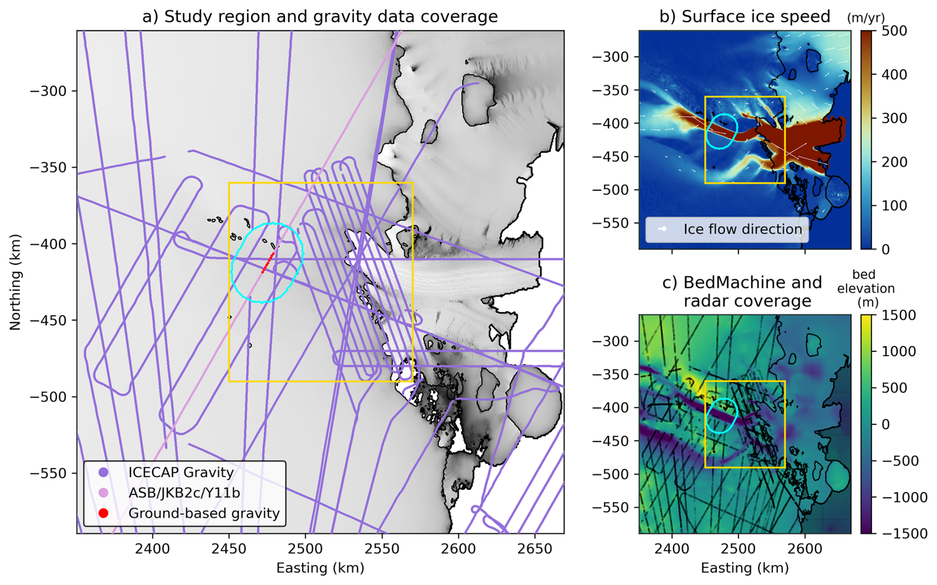
Figure 1 Overview of the Denman Glacier region. (a) Airborne survey coverage and outlines of target areas for regional (yellow rectangle) and local (light blue oval) inversion. (b) Surface speed and flow directions from MEaSUREs (Rignot et al., 2019b). (c) Bed topography from BedMachine v3 (Morlighem et al., 2020) with ICECAP RES bed pics and bathymetry in light gray, including ice-free land boundaries and ice shelf outlines.

Because much of the Denman system is grounded below sea level (Morlighem et al., 2020) (Fig. 1c), the glacier is especially sensitive to changes in ice–ocean interactions and basal conditions, which could amplify its sea level contribution under a warming climate (Pelle et al., 2023). If the Denman Glacier retreats irreversibly, it could ultimately contribute up to 1.5 m of global sea level rise (Rignot et al., 2019a). Recent multidecadal analyses indicate an acceleration in ice flow speed, with an estimated increase of 174 ± 4 % in its grounded portion and 36 ± 5 % in its floating portion in the last 50 years (Miles et al., 2021), while the grounding line has retreated more than 5 km since 1996 (Brancato et al., 2020). Grounding line flux is highly sensitive to ice thickness, with Schoof (2007) demonstrating that the steady-state flux increases nonlinearly with thickness for deformation-dominated flow. In fast-sliding regimes modeling studies have shown a significant sensitivity of grounding line retreat to bed depth changes (Pattyn et al., 2012; Seroussi et al., 2014).

Topography also provides critical insight into the tectonic and erosional history of the region. Reaching over 900 km landwards, the Denman glacier catchment is suggested to lie on top of the Knox Rift, which is interpreted to be a failed rift from the separation of India from East Gondwana (Aitken et al., 2014) with a significant sedimentary infill of 6 to 7 km (Maritati et al., 2016).

Despite targeted ICECAP aerogeophysical/radar acquisitions (Young et al., 2011) (Fig. 1a) that improved regional context significantly, radar bed observations in the Denman region are still sparse and uneven, especially in the deep, narrow marine trough, near the grounding zone, and non-existent beneath the ice shelf. These gaps (Fig. 1c) reflect the difficult radar-imaging environment, rather than limitations of any specific survey: the deep and narrow marine trough, steep valley walls, crevasse fields, and floating ice all reduce the ability of any radio-echo sounding (RES) system to image the bed. Off-nadir returns and layover are common (Peters et al., 2005), while warm or attenuating ice, water-saturated sediments, and rough basal interfaces weaken or de-correlate the bed echo (Matsuoka et al., 2012; Jordan et al., 2017; MacKie et al., 2021; Franke et al., 2022). As a result, along-track bed picks are often discontinuous and their quality varies; between tracks, often spaced by many kilometers, bed elevations must be interpolated or extrapolated, producing anisotropic errors that are small along flight lines but grow rapidly away from them (Morlighem et al., 2020). Additional systematic uncertainties arise from poorly constrained radar velocity/firn corrections and from ambiguities when multiple reflectors (e.g., internal layers vs. bed) are present (King, 2020). Together, these factors yield bed estimates with spatially variable, directionally biased uncertainty, especially near the grounding zone where accurate topography matters most.

Antarctic bed compilations reconcile heterogeneous radar coverage by spatial interpolation (e.g., Bedmap2; Fretwell et al., 2013) smoothing sharp relief and “bridging” across steep troughs, which can underestimate depth and sidewall steepness. By contrast, streamline-guided interpolation in Bedmap3 (Pritchard et al., 2025) suggests a ∼ 2.5 km deep trough beneath the Denman Glacier by explicitly following ice-flow trajectories between observations to preserve along-trough continuity and sharpen outlet geometry at the margins improving fidelity in many coastal sectors. However, this approach also has limitations: ice thickness is linearly interpolated along each streamline where radar measurements are available and may consequently underestimate the true bed elevation. Mass conservation approaches (BedMachine; Morlighem et al., 2020), fuse radar thickness with satellite ice velocities and surface mass balance to infer bed between tracks, and can recover very deep, narrow troughs notably the Denman trough exceeding ∼ 3.5 km below sea level in their interpretation (Fig. 1c). A recently developed mass conserving, geostatistical MCMC framework (Shao et al., 2026) further demonstrates that multiple, equally plausible bed geometries can satisfy both the mass-flux constraints and radar observations, producing ensembles with much greater small-scale roughness and uncertainty than deterministic inversions used for, e.g. BedMachine. Applied to Denman Glacier, this approach reveals kilometer-scale differences from BedMachine, showing that mass-conserving solutions remain highly non-unique while retaining realistic roughness. The benefits of this approach weaken where surface velocity gradients are small, contributing to much of the spread among regional products in this area. This motivates adding independent constraints, such as gravity, which provides a complementary approach that is insensitive to ice dynamics and instead reflects the mass distribution of ice and deeper subsurface.

Several studies have demonstrated that free-air gravity disturbances can be used effectively to model three-dimensional subglacial topography and bathymetry beneath ice shelves (e.g., Charrassin et al., 2025; Hodgson et al., 2019), where the presence of floating ice severely hampers radar imaging due to scattering and absorption of the radar signal by the ocean beneath the ice shelf. Even in the presence of RES bed data, gravity data provides some sensitivity to 3D structure and off-profile features and can guide reconstruction of the surface. However, the gravity signal integrates over depth and is inherently non-unique, meaning that recovered structures depend on assumptions about the background geology and density distribution. Variations in crustal properties or unmodeled geological heterogeneity can therefore bias inferred bed geometry (Tankersley et al., 2025; An et al., 2019; Charrassin et al., 2025).

In the region of the Denman Glacier Trough, Maritati et al. (2016) utilized ICECAP airborne gravity data to model subglacial geology and density distribution, identifying a maximum sediment basin thickness of 6.5 km. Their results indicate higher densities in Indo-Antarctica (2.7 g cm⁻³) and lower densities in Australo-Antarctica (2.5–2.7 g cm⁻³) in general agreement with Lösing et al. (2025b). Maritati et al. (2016) further argue that the presence of a mechanically weak and potentially water-saturated bed (Wright et al., 2012; Gooch et al., 2016) may have facilitated focused ice flow along a pre-existing rift structure, similar to observations in West Antarctic ice streams (Bingham et al., 2012). Their structural interpretation aligns with the crustal framework of Aitken et al. (2023), who map the western flank of the trough as crystalline basement and the eastern flank as a relatively young sedimentary basin. Exposures of the Sandow Group with low-grade metasedimentary rocks mapped around Bunger Hills/Denman help explain the subdued magnetics and gravity lows there (Aitken et al., 2016; Mikhalsky et al., 2020).

To better constrain the subglacial topography and geological structure in this key region, we collected ground-based gravity data at nine sites during the Denman Terrestrial Campaign 2023/24 along a transect of about 14 km in length along ICECAP flight line ASB/JKB2c/Y11b across the Denman Glacier system (Fig. 1a). These ground measurements sit at the ice surface and retain short-wavelength gravity signals that are otherwise suppressed at aircraft altitude by mandatory along-track filtering and upward continuation; they also offer tighter drift control/base ties. Airborne gravity is excellent for regional context but prone to smoothing small-scale features. Our ground survey therefore complements the airborne archive by restoring short-wavelength amplitude, reducing local uncertainty, and providing an independent check on bed depths inferred between radar tracks. It also provides valuable constraints for interpreting the crustal structure and sedimentary architecture underlying the glacier. In combination with ICECAP RES, airborne gravity, and magnetic data, we model the subglacial topography and place the Denman Glacier into the regional context using the probabilistic Markov Chain Monte Carlo framework of Field et al. (2026). For an under-determined problem such as gravity inversion, this method can jointly explore a wide range of possible subsurface geometries and quantify the non-uniqueness of the bed solutions. To capture both the broader structural controls and the fine-scale trough geometry, we perform a two-scale inversion: a regional, lower-resolution inversion that constrains the long-wavelength architecture, and a local, higher-resolution inversion focused on the ground-based transect, resolving sharper gradients and short-wavelength bed variability that cannot be recovered from airborne data alone (Fig. 1a).

2 Data

2.1 ICECAP data

We use the airborne geophysical data from the ICECAP-I and EAGLE/ICECAP-II surveys from 2008–2009 through to 2016–2018 seasons (Aitken and Nigro Rodrigues Alves Ramos, 2020; Blankenship et al., 2011, 2012, 2014; Roberts et al., 2018, 2025) including magnetics, gravity, and radio-echo sounding (RES) bed topography data, supplemented by Bedmap3 bed topography point data (Frémand et al., 2023). The ICECAP project collected data over East Antarctica using a Basler BT-67 aircraft (C-JKB) equipped with a Geometrics 823A magnetometer, and depending on the campaign, a LaCoste & Romberg (L&R) BGM-3 (early campaigns) or a Canadian Micro Gravity (CMG) GT-1A (later campaigns) gravimeter, HiCARS and later HiCARS-2 RES systems, and Riegl LD90-3800 HiP-LR Laser Altimeter. Surveys were conducted at varying aircraft heights, typically ranging from approximately 1.5 km up to ∼ 4 km ellipsoidal heights, and at average speeds around 80–90 m s⁻¹, with survey lines variably spaced from 10 to 50 km apart. Coverage is moderate, with close data around the grounding line, but major data gaps in the inland region (Fig. 1).

ICECAP airborne gravity data have cross-over residuals typically in the range of 1 to 3 mGal after line-levelling (Blankenship et al., 2014). RES data typically carry 10 to 30 m uncertainty under good bed returns, increasing locally up to ∼ 50 m in areas of weak or multi-path echoes, steep bed slopes, or strong clutter (Blankenship et al., 2012). Aitken et al. (2020) reprocessed the magnetic data (Aitken and Nigro Rodrigues Alves Ramos, 2020) with a median crossover error of 5 nT. We discarded all ICECAP data flagged with aviation turns.

2.2 Ground-based gravity data

On 7 January 2024, we collected nine ground-based gravity measurements along a ∼ 14 km transect across the Denman Glacier (Fig. 1a, spacing ≈ 1.7 km) to recover short-wavelength anomalies. For this, we used a Scintrex CG-5 Autograv (resolution 0.001 mGal; typical station repeatability of 5 µGal under stable conditions; long-term drift below 0.02 mGal d⁻¹; Scintrex Limited, 2017), with daily base ties at Bunger Hills and loop closures including the Casey absolute site to control drift.

Field readings from the CG-5 (y_raw) were first tied to an absolute reference by calibrating against the Casey Station fundamental value g_fund = 982 380.48867 mGal (Lon: 110.5226, Lat: −66.2820, height: 19 m, positional error: 3 m, gravity error: 30 µGal). We modeled the instrument drift by fitting a baseline f(t) to repeated measurements of the base station at Casey and three different stations at Bunger Hills and evaluating this baseline at each observation time t_i (linear interpolation between base ties, Fig. A1). The interpolated baseline y_base(t_i)=f(t_i) represents the predicted CG-5 reading due solely to drift at time t_i. We then applied a time-dependent offset C(t_i)=g_fund−y_base(t_i) to each reading to obtain the absolute observed gravity

$$\begin{array}{}\text{(1)}& g_{\mathrm{obs}}\left(t_i\right)=y_{\mathrm{raw}}\left(t_i\right)+C\left(t_i\right).\end{array}$$

Station coordinates were determined from dual-frequency Trimble GNSS. Rover trajectories were post-processed kinematically (PPK) in Emlid Studio v1.5 (Emlid Ltd., 2023); the local PPK network was tied to an AUSPOS (ITRF2014) solution (Geoscience Australia, 2024). On the Glacier, we positioned one GNSS Antenna at a mid-line base (Lon: 99.4622, Lat: −67.1976, height: 804.817 m ellipsoidal) for ∼ 7 h. We used the ellipsoidal heights to provide the vertical control needed for accurate normal-gravity/free-air corrections.

We then computed the normal gravity γ(Φ,h) on the WGS84 reference ellipsoid at each station's geodetic latitude Φ and ellipsoidal height h_e using Boule's closed-form normal-gravity implementation (Fatiando a Terra Project et al., 2024a). This already includes the free-air term, so no separate FA correction is added. Finally, we formed the free-air anomaly as

$$\begin{array}{}\text{(2)}& \mathrm{\Delta }g=g_{\mathrm{obs}}-\mathit{\gamma }(\mathrm{\Phi },h_{\mathrm{e}})+g_p+g_{\mathrm{tidal}},\end{array}$$

where g_tidal is a recomputed solid-Earth tide using a python library by Leeman (2023), based on Longman (1959), replacing any tide the instrument applied. g_p is the atmospheric-pressure correction of 0.3 µGal hPa⁻¹ (Falk et al., 2020) applied to the station pressure anomaly relative to a campaign reference (Bunger Hills archive mean in February was near 981.14 hPa; Bureau of Meteorology, 2000; for January no data was available).

2.3 Application of DC Shifts

To bring the ICECAP airborne and our ground-based gravity measurements onto a consistent datum, we estimated and applied constant (DC) shifts relative to the most recent Antarctic Gravity Anomaly Grid (AntGG) compilation (Scheinert et al., 2024; Zingerle et al., 2021). We used the 5 km resolution AntGG2021 product, which represents a major update of the earlier AntGG2016 release (Scheinert et al., 2016). AntGG2021 integrates airborne and terrestrial gravity observations (including ICECAP data) into a continent-wide homogenized compilation making it a suitable reference field. For each dataset, we compared the observations to the AntGG2021 gravity disturbance field by upward-continuing AntGG2021 from the surface to the ICECAP observation height using the workflow described in Sect. 2.5. For the ground-based transect, no upward continuation was required, as the data are already at (near-)surface elevation. In both cases, the mean difference was calculated and applied as a constant shift. These shifts were then applied to ICECAP (11 mGal) and ground-based (14 mGal) gravity disturbances to align them with the AntGG2021 reference frame. Along the ground-based transect, however, a significant local mismatch between the ICECAP airborne gravity and both the AntGG2021 reference field, and the ground-based observations persisted after application of the regional correction. Therefore, for the profile comparison shown in Fig. A2, an additional local adjustment of 26 mGal was applied to the ICECAP data in this limited area to ensure consistency with the AntGG2021 field at the local flight altitude and to facilitate comparison with the ground-based measurements. This local correction was only applied along the transect and not to the wider airborne dataset.

2.4 Isostatic correction

Both ICECAP and ground-based datasets report free-air gravity anomalies relative to the ellipsoid. Keeping the geodetic convention (Hackney and Featherstone, 2003), we refer to these quantities throughout as gravity disturbances (Δg). To isolate signals associated with near-surface mass anomalies, we remove the isostatic Moho contribution g_iso (Fig. 3e) from both datasets. The isostatic correction is based on Airy compensation of the rock-equivalent topography (using BedMachine v3 Morlighem et al., 2020), obtained by compressing the ice column to a rock density of ρ_rock=2750 kg m⁻³ (based on the median density of collected in-situ rock samples from the Denman Terrestrial Campaign and previous field trips; Lösing et al., 2025a; Fig. 3h). We assume a crust–mantle density contrast of 400 kg m⁻³ and a reference Moho depth of 40 km, consistent with Haas et al. (2023). The gravity effect of the resulting Moho relief is forward-modeled using the adaptive cuboids method of Liebsch (2020) and evaluated at the respective observation heights of the airborne and ground-based gravity datasets. This procedure approximates the long-wavelength mass variations expected under near-isostatic equilibrium, thereby isolating deeper contributions to the gravity field. While the true Moho may deviate locally from the Airy prediction, this does not significantly affect the long-wavelength component emphasized here. The resulting isostatically corrected gravity disturbance is given by

$$\mathrm{\Delta }{g}_{\mathrm{iso}}\left(\mathit{x}\right)=\mathrm{\Delta }g\left(\mathit{x}\right)-g_{\mathrm{iso}}\left(\mathit{x}\right).$$

The correction was applied separately to the original ICECAP and ground-based point observations. For each observation, g_iso was evaluated at its original horizontal coordinates and observation height and subtracted from the corresponding gravity disturbance.

2.5 Upward continuation and merging

To enable consistent comparison and inversion, we resampled the BedMachine topography onto reference grids at 1 and 2 km resolution for a high-resolution Denman Trough and lower-resolution regional inversion, respectively. Continuous fields were resampled using block-median reduction, while categorical fields were assigned by nearest-neighbour interpolation. We followed Field et al. (2026), and upward-continued the corrected ICECAP observations to a uniform observation height of 3.5 km above the WGS84 ellipsoid using gradient-boosted equivalent sources, as implemented in the open-source Python package Harmonica (Soler and Uieda, 2021; Project et al., 2023). We use optimized parameters by cross-validation for damping $\mathit{\lambda }\in \mathit{\{}\mathrm{0.1},\mathrm{1},\mathrm{100}\mathit{\}}$ and source-depth $d\in \mathit{\{}\mathrm{1},\mathrm{2},\mathrm{3}\mathit{\}}$ km with the best solution at λ=0.1 and d=1 km. The upward-continued gravity was then evaluated directly at the nodes of the resampled BedMachine reference grids, and cells farther than 2 km from the nearest original observation were masked. This conservative masking ensures that only values directly supported by observations are retained, avoiding artifacts from equivalent-source extrapolation and preventing the inversion from fitting unconstrained regions or producing overly smooth results. The radar bed picks were gridded onto the same reference grids using a 2D spatial binning approach. Point coordinates were assigned to grid cells whose boundaries were computed from the BedMachine Easting and Northing edges, and the mean bedrock altitude within each cell was computed to produce a rasterized field that was used to condition the inversion.

Next, the corrected ground-based gravity data are incorporated. The observation grid height was set to measured ice surface for the ground-based data. The nearest grid cells along the ground transect were explicitly identified using a nearest-neighbour search with a maximum distance threshold of 800 m. For each ground observation, the corresponding grid value in the upward-continued airborne gravity field was identified, and the transect gravity value and its associated observation height were added. This ensured that the nine ground gravity measurements were retained explicitly in the inversion dataset.

3 Methods

In order to resolve the region's bed topography, we need to isolate and remove the non-terrain gravity disturbance, while recognizing the uncertainty in geology and crustal density variations. As a first step, we use sequential Gaussian simulation (SGS) (Deutsch and Journel, 1997) to generate an ensemble of targeted terrain effects (i.e., Bouguer corrections) for inversion (Sect. 3.1). Subsequently, we perform one low-resolution regional inversion and one high-resolution local inversion using an MCMC framework to solve possible terrain geometries (Sect. 3.2). To aid interpretation, we also calculate the Depth to the Magnetic Sources with Euler deconvolution (Melo and Barbosa, 2020, Sect. 3.4).

3.1 Geostatistical separation of terrain and non–terrain effects

Our goal is to remove non–terrain contributions from the gravity observations so that the inversion is driven primarily by the terrain effect of unresolved bed geometry within the inversion domain. We therefore (i) forward–model and subtract the known terrain effect from the isostatically corrected gravity disturbance to obtain a non–terrain disturbance; (ii) estimate its long-wavelength component by fitting a smooth trend to selected conditioning observations with reliable, radar-based topographic control; (iii) subtract the fitted trend from the non-terrain disturbance, transform these residuals to normal scores and estimate their spatial covariance; (iv) simulate an ensemble of spatially correlated residual fields and add these back to the trend to obtain plausible non–terrain distubances; and (v) subtract each non–terrain field from the isostatically corrected gravity disturbance to obtain the ensemble of target terrain effects used for inversion (Fig. 2). In particular, the separation of long-wavelength non-terrain gravity contributions from the shorter-wavelength terrain signal is conceptually similar to the DC-shift approach of An et al. (2019) and the constraint-point regionalization approach of Tankersley et al. (2025). However, the regional field is estimated differently in the following steps.

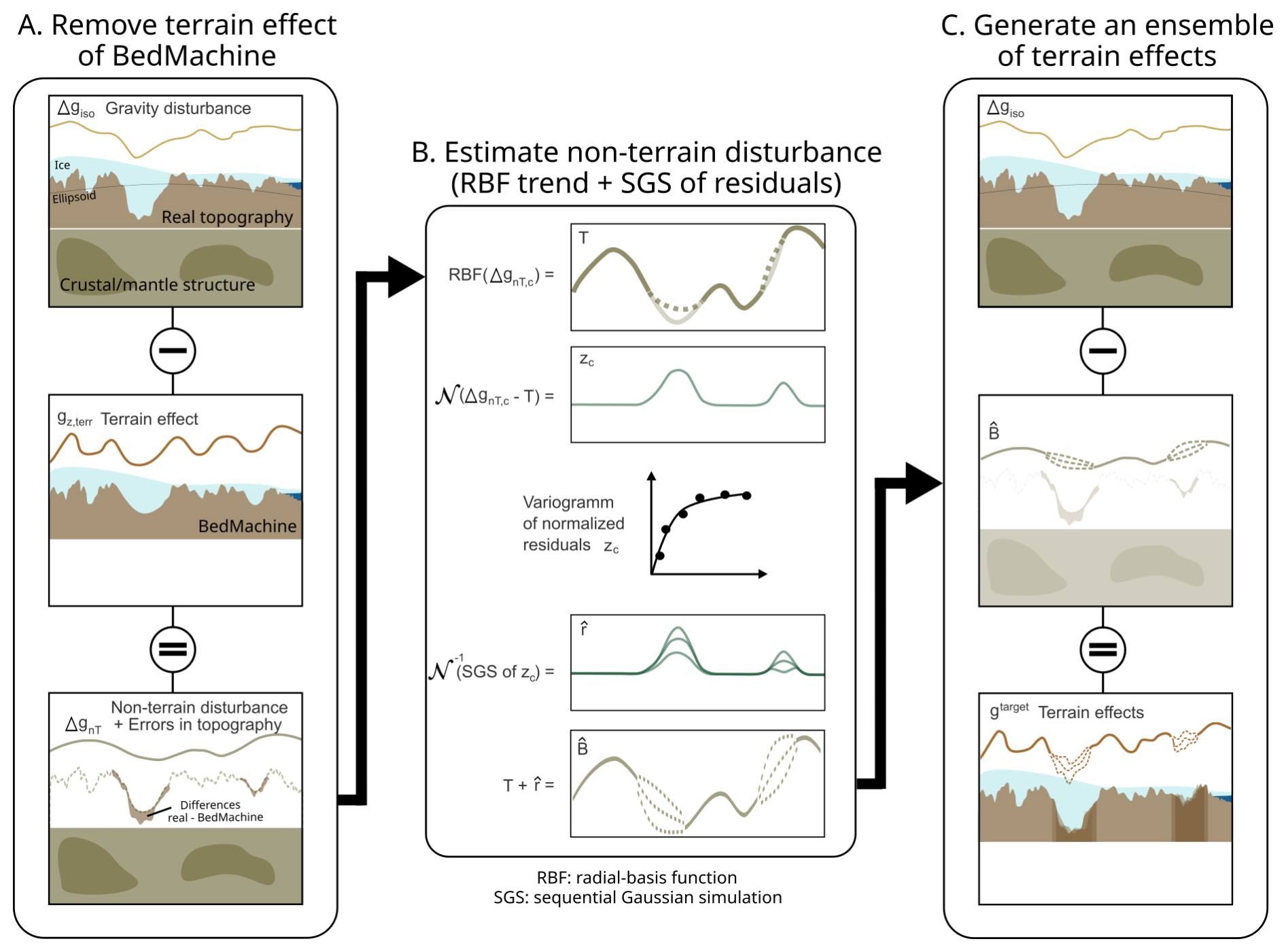
Figure 2 Schematic of the isolation process of non-terrain gravity disturbances and terrain effects and the propagation of uncertainties in the regional background gravity field. (A) Subtracting the terrain correction (g_z,terr) based on BedMachine from the isostatically corrected gravity disturbance (Δg_iso) yields a non-terrain disturbance (Δg_nT), but errors or biases in the prescribed topography map directly into the residual signal. (B) Instead of relying on a fixed bed, we decompose the non-terrain field into a smooth regional trend (T), estimated using a radial-basis function (RBF), and a short-wavelength residual component. The residuals within regions lacking independent topographic constraints are transformed to a normal-score domain (z_c), characterized using a variogram model, and stochastically simulated using sequential Gaussian simulation (SGS) to generate an ensemble of plausible residual realizations. Following inverse transformation, these residual realizations ($\widehat{r}$) are added back to the regional trend to obtain an ensemble of reconstructed non-terrain fields ($\widehat{B}$). (C) Removing this from the isostatically corrected gravity, we obtain an ensemble of target terrain effects, capturing the uncertainty arising from poorly constrained non-terrain gravity contributions and unresolved topography. More details and step-by-step descriptions are in the text.

3.1.1 Step i: Remove the terrain effect based on BedMachine (Fig. 2A)

We compute the vertical gravity from “known” surface and bed topography (BedMachine v3; Morlighem et al., 2020) using a prism formulation (Fatiando a Terra Project et al., 2024b) with fixed densities for ice and seawater (ρ_ice=917 kg m⁻³, ρ_seawater=1027 kg m⁻³). Rock density ρ_rock is spatially variable and taken from the 3D joint gravity–magnetic inversion by Lösing et al. (2025b) (mean over the upper 20 km, Fig. 3h). The domain is tessellated into right-rectangular prisms with footprints equal to the grid spacing and vertical extents bounded by the mapped surfaces in BedMachine. For each grid cell, separate prisms are generated for ice, water, and rock, partitioned into components above and below the reference ellipsoid. This results in up to six prism groups: ice above the ellipsoid, ice below the ellipsoid, water above the ellipsoid, water below the ellipsoid, bedrock above the ellipsoid, and compensating negative-density bedrock prisms below the ellipsoid. Below z=0 m, densities are assigned as contrasts (e.g., ρ_ice−ρ_rock). The gravity contribution of each prism is computed analytically and summed at the respective gravity observation locations and elevations to obtain the predicted terrain effect, denoted g_z,terr(x).

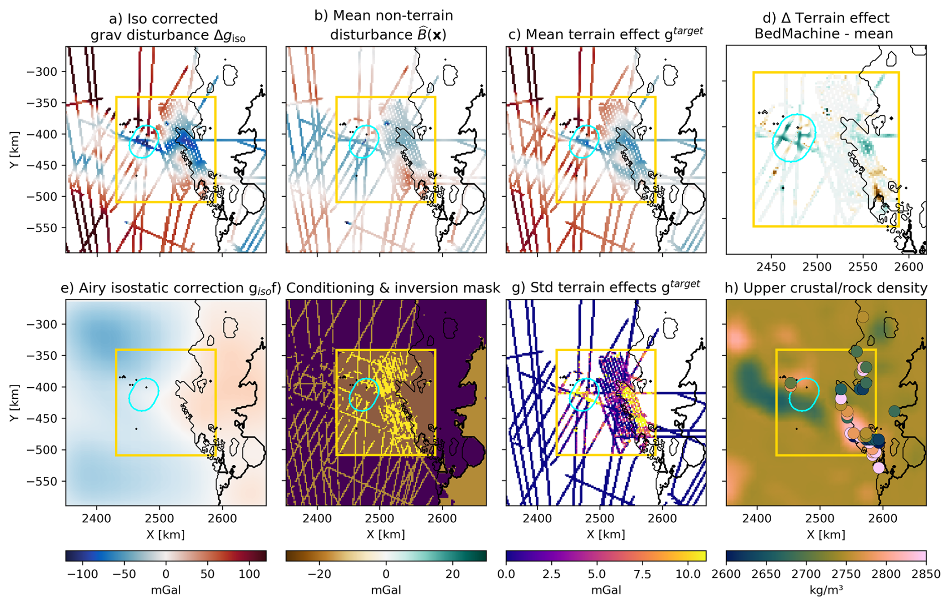
Figure 3 Overview of the gravity field decomposition and inversion inputs. (a) Isostatically-corrected gravity disturbance Δg_iso. (b) Mean estimated non-terrain gravity disturbance $\widehat{B}$ and (c) mean target terrain effect g^target. Both were obtained by the workflow described in Sect. 3.1 and Fig. 2. (d) Difference between the BedMachine-derived terrain effect and the mean target terrain effect. (e) Airy isostatic correction g_iso used to produce Δg_iso. (f) Conditioning and inversion masks used in the gravity inversion. (g) Standard deviation of the target terrain effects derived from the ensemble of sequential Gaussian simulations, representing uncertainty in the non-terrain correction. (h) Spatially variable upper-crustal density field by Lösing et al. (2025b) with 5 km binned in situ density observations (Lösing et al., 2025a) shown as circles. The golden rectangle and cyan contour indicate the regional and local trough inversion domains, respectively. Black contours show the ice shelf extent and ice-free land boundaries derived from BedMachine v3.

Subtracting this from the isostatically corrected gravity disturbance Δg_iso (Fig. 3a) yields

$$\begin{array}{}\text{(3)}& \mathrm{\Delta }{g}_{\mathrm{nT}}\left(\mathit{x}\right)=\mathrm{\Delta }{g}_{\mathrm{iso}}\left(\mathit{x}\right)-g_{z,\mathrm{terr}}\left(\mathit{x}\right),\end{array}$$

which we interpret as the observed non–terrain disturbance. This field contains long-wavelength contributions from regional geology and any remaining signals not explained by mapped topography.

3.1.2 Steps ii–iv: Estimation of the non–terrain component (Fig. 2B)

Step ii: Smooth background trend for the non–terrain disturbance

Let $\mathit{\{}{\mathit{x}}_{\mathrm{c}},\mathbf{\Delta }{\mathit{g}}_{\mathrm{nT},\mathrm{c}}\mathit{\}}$ be the conditioning subset (Fig. 3f), consisting of all non–terrain disturbance grid points outside the inversion domain and, within the domain, only those co-located with radar picks (i.e., locations with independent bed control).

We estimate a regional trend T(x) by fitting a smoothing radial-basis function (RBF; SciPy RBFInterpolator) to Δg_nT,c at x_c, using a large Tikhonov regularization parameter (λ=10¹⁰) to enforce a smooth, long-wavelength field. Residuals are then

$$\begin{array}{}\text{(4)}& {\mathit{r}}_{\mathrm{c}}=\mathbf{\Delta }{\mathit{g}}_{\mathrm{nT},\mathrm{c}}-T\left({\mathit{x}}_{\mathrm{c}}\right).\end{array}$$

Although T is fitted only to the conditioning subset, it is evaluated at all observation locations in subsequent steps.

Step iii: Gaussian residual and spatial variogram

Because sequential Gaussian methods assume normally distributed variables, we apply a normal-score transform to r_c to obtain standardized scores z_c. We compute a directional experimental variogram of z_c using logarithmically spaced lag distances (order 1–100 km), and fit an exponential variogram model with geometric anisotropy (azimuth −20°; minor range set to one third of the major range). The fitted variogram parameters (nugget = 0, sill = 1.07, major range = 26 km, minor range = 8.8 km) are obtained from automatic estimation in scikit-gstat (Mälicke, 2022) and define the spatial covariance of the residual non–terrain field.

Step iv: Reconstructing short-wavelength non–terrain structure

Using the fitted covariance model, we reconstruct the short-wavelength residual over all observation locations by sequential Gaussian simulation (SGS) in the normal-score domain (MacKie et al., 2023). At each prediction node, a local neighbourhood (up to k=20 neighbours within a 50 km search radius) is used to solve the ordinary kriging system, yielding the local conditional mean and variance. A Gaussian draw from this distribution provides the simulated value, which is then appended to the conditioning set as the simulation proceeds along a random path. The simulated scores are inverse-transformed back to physical units to obtain $\widehat{r}\left(\mathit{x}\right)$. Repeating SGS with different random seeds produces an ensemble of plausible residual fields and associated uncertainty.

3.1.3 Step v: Assembling the non–terrain disturbance (Fig. 2B) and extracting the target terrain effect (Fig. 2C)

Our estimate of the non–terrain disturbance is given by the sum of the smooth trend and simulated residuals (Fig. 3b),

$$\begin{array}{}\text{(5)}& \widehat{B}\left(\mathit{x}\right)=T\left(\mathit{x}\right)+\widehat{r}\left(\mathit{x}\right),\end{array}$$

representing a plausible realization of the non–terrain disturbances.

Subtracting these from the isostatically corrected gravity disturbance yields the target terrain effects (Fig. 3c),

$$\begin{array}{}\text{(6)}& g^{\mathrm{target}}\left(\mathit{x}\right)=\mathrm{\Delta }{g}_{\mathrm{iso}}\left(\mathit{x}\right)-\widehat{B}\left(\mathit{x}\right),\end{array}$$

which isolate the portion of the gravity field attributable to unresolved terrain (i.e., bed geometry variations within the inversion domain). The residual terrain effect (Fig. 3d), calculated as the difference between the BedMachine-derived terrain effect and the mean target terrain effect, provides a first indication of where the prior bed model could differ most from the gravity-derived bed. These differences are particularly pronounced within the trough region and motivate the subsequent gravity inversion for bed topography. The SGS step preserves realistic variance and spatial structure of the non–terrain disturbance; its ensemble allows propagation of regional–field uncertainty into the inversion (Fig. 3g). In total, we generate an ensemble of 100 plausible terrain effects for the regional, and 50 for the local inversion.

3.2 MCMC gravity inversion and conditional random fields

To infer subglacial topography and its uncertainty in the Denman Glacier region, we employ a Markov Chain Monte Carlo (MCMC) approach following Field et al. (2026), which iteratively adjusts a model of the subglacial bed to minimize discrepancies between observed and modeled gravity disturbances.

We initialize the process by using bedrock topography (h₀) based on BedMachine (Morlighem et al., 2020) plus a smooth Gaussian random perturbation. Gravitational predictions are then again computed using the forward model that integrates gravitational effects of prisms derived from the generated topography (Sect. 3.1). Here, we use the constant ρ_rock=2750 kg m⁻³.

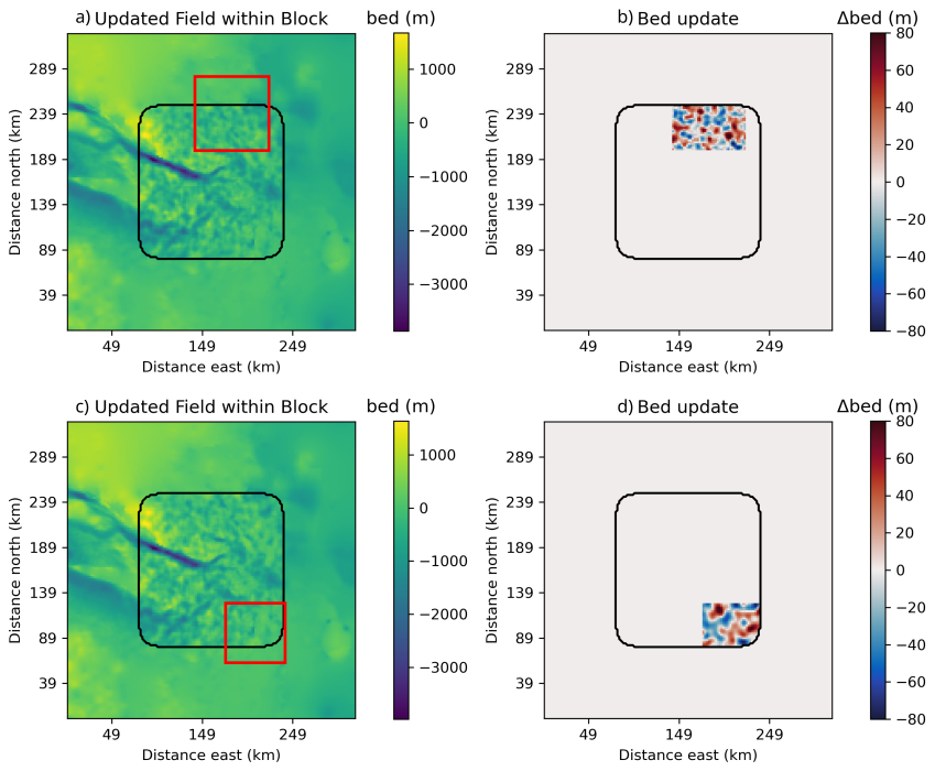
Figure 4 Localized bed updates inside the inversion mask. Panels (a) and (c) show the updated bed elevation over the full map area with the inversion mask boundary outlined in black; the small red rectangle in each denotes the stencil in which the local update was applied. Panels (b) and (d) show the corresponding bed-change maps (Δbed): the coloured patch shows the non-zero update. (a–b) Example with b=41, d_c=5, v=100; (c–d) example with b=33, d_c=10, v=100. Updated beds are clipped to be only applied inside the inversion mask.

At each iteration, we make a small, local change to the bed (Fig. 4). We pick a random cell inside the inversion mask, form a b×b stencil around it, and add a zero-mean Gaussian patch only within that stencil:

$$\begin{array}{rl}& \mathit{\delta }\mathit{h}\sim \mathcal{N}\left(\mathbf{0},s(v{)}^{\mathrm{2}}\mathbf{K}\right),s\left(v\right)\equiv {\displaystyle \frac{v}{\mathrm{3}}},\\ & K_{ij}=\exp \left(-{\displaystyle \frac{\Vert {\mathit{p}}_i-{\mathit{p}}_j{\Vert }^{\mathrm{2}}}{d_{\mathrm{c}}}}\right)+\mathit{\epsilon }{\mathit{\delta }}_{ij},\end{array}$$

where p_i,j are stencil index coordinates (in grid-cell units). The matrix K sets the spatial correlation in the patch; d_c controls how smooth/broad it is (larger d_c meaning smoother, broader), and ε is a tiny nugget for numerical stability. The scale s sets the proposal amplitude (derived from the perturbation strength v). We add δh to the current bed inside the stencil; outside, the bed is unchanged. The parameters we used in the inversion are listed in Table 1.

Table 1 Stencil update parameters used in the inversion. Each set defines the stencil size b, correlation control d_c, perturbation strength v, and number of iterations n.

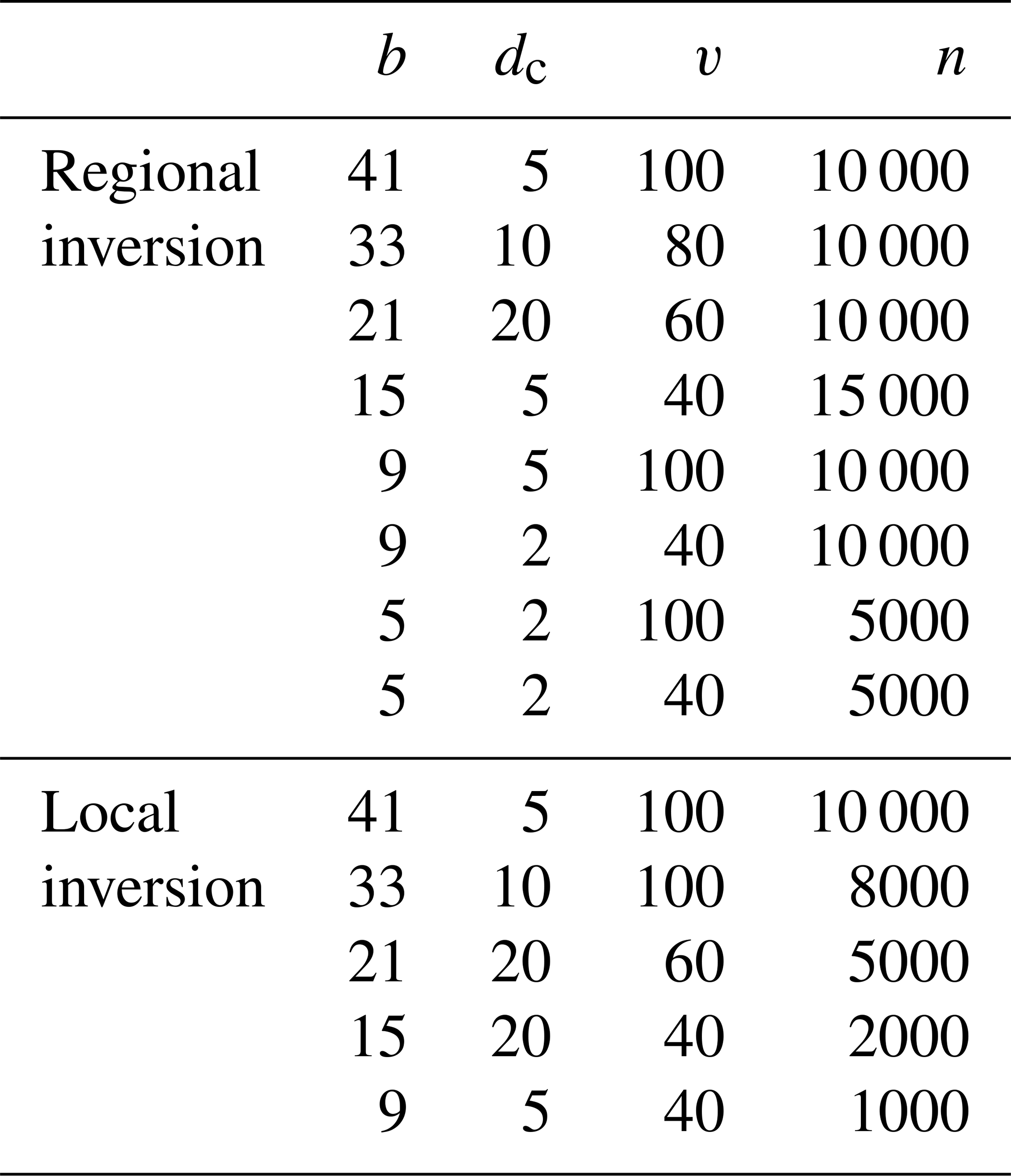
By progressing from large to small update stencils, the multiscale scheme fits the long-wavelength geometry early and incrementally adds finer detail, reconciling the model with the coarse airborne ICECAP coverage and the heterogeneous radar and ground-gravity constraints.

Proposals are clipped to remain physically plausible (e.g., below the ice surface by a small buffer to account for uncertainties). For efficiency, we recompute forward gravity g^pred only at observation points within 10 km of the updated patch and insert this change into the full prediction.

Acceptance uses a Metropolis criterion based on a joint loss ℒ(h), that combines gravity and radar bed picks (within the updated patch), by prescribed uncertainties. For a bed field h and a proposal ${\mathit{h}}^{\prime }=\mathit{h}+\mathit{\delta }\mathit{h}$, we define

$$\mathcal{L}\left(\mathit{h}\right)={\mathit{\chi }}_g^{\mathrm{2}}\left(\mathit{h}\right)+\mathit{\mu }{\mathit{\chi }}_h^{\mathrm{2}}\left(\mathit{h}\right),$$

with

$$\begin{array}{rl}& {\mathit{\chi }}_g^{\mathrm{2}}\left(\mathit{h}\right)=\sum _{i\in {\mathcal{I}}_g}{\left({\displaystyle \frac{g_i^{\mathrm{target}}-g_i^{\mathrm{pred}}\left(\mathit{h}\right)}{{\mathit{\sigma }}_g}}\right)}^{\mathrm{2}},\\ & {\mathit{\chi }}_h^{\mathrm{2}}\left(\mathit{h}\right)=\sum _{k\in {\mathcal{I}}_h}{\left({\displaystyle \frac{h_k-h_k^{\mathrm{radar}}}{{\mathit{\sigma }}_h}}\right)}^{\mathrm{2}}.\end{array}$$

Here ℐ_g indexes all gravity stations and ℐ_h indexes radar–controlled bed cells inside the updated block. h^radar is the bed elevation from radar, and σ_g and σ_h are the adopted data uncertainties, which we set to σ_g=1.5 mGal and σ_h=30 m, in the range of expected uncertainties (Sect. 2.1). μ is a dimensionless weight controlling the gravity–vs–radar trade-off, which is set to 1. In this formulation, the gravity and radar terms enter the likelihood with equal prominence per unit misfit, meaning that any imbalance in uncertainty estimates (e.g., underestimated radar noise or spatially variable gravity errors) could shift the inversion towards favouring one dataset over the other.

The Metropolis acceptance probability is $\mathit{\alpha }=min\left\{\mathrm{1},\exp \left[-\frac{\mathrm{1}}{\mathrm{2}}\left(\mathcal{L}\left({\mathit{h}}^{\prime }\right)-\mathcal{L}\left(\mathit{h}\right)\right)\right]\right\}$. A random drawing from a uniform distribution decides whether the updated model is accepted. Accepted proposals replace the current state (${\mathit{h}}^{\prime }\to \mathit{h}$), otherwise the previous state is retained. Iterating this procedure yields a Markov chain of bed realizations that are jointly consistent with the gravity data and, when enabled, the radar constraints. To quantify sensitivity to stochastic choices and to obtain uncertainty bounds, we repeat the full inversion for each target terrain effect g^target, yielding 100 regional and 50 local bed realizations. Each repetition uses an independent random seed for both the conditional Gaussian-field initialization and the block–proposal sequence.

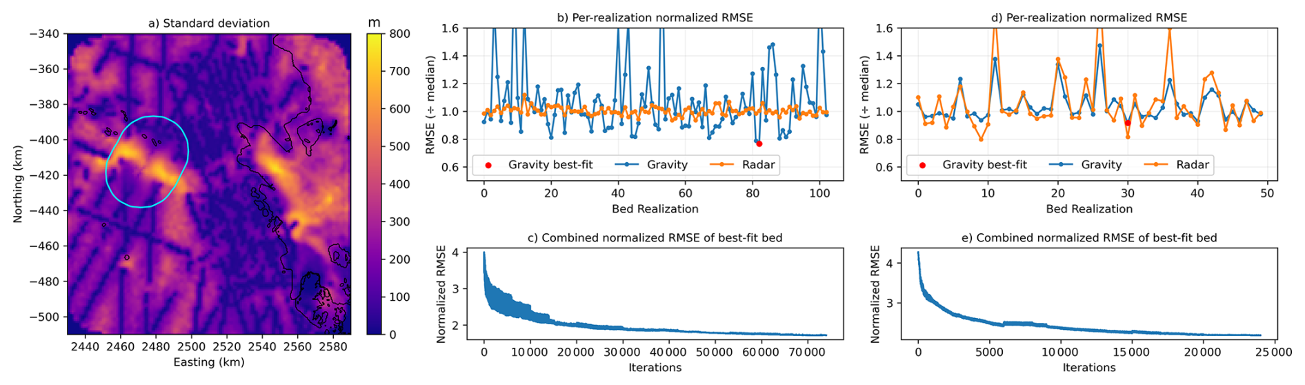
Figure 5 (a) Ensemble standard deviation of inferred bed elevation. (b, d) Normalized RMSE for each bed realization, regional low-resolution and local high-resolution, respectively, showing individual misfits to gravity (blue) and radar (orange) data, and highlighting the realization selected as the gravity best-fit model (red dots). (c, e) Evolution of the combined normalized RMSE during the MCMC iterations for the best-fit bed, regional low-resolution and local high-resolution, respectively, illustrating the convergence behaviour of the inversion. Black contours show the ice shelf extent and ice-free land boundaries derived from BedMachine v3.

Because the MCMC framework introduces stochastic bed perturbations throughout the inversion mask, small-scale bed undulations in areas far from gravity observations are poorly constrained and should therefore be interpreted cautiously. To quantify this uncertainty, we compute the ensemble standard deviation of accepted bed realizations (Fig. 5a) and use it as a measure of spatial model variability. This uncertainty estimate provides a quantitative assessment of the reliability of the inferred bed geometry. At the same time, the stochastic framework permits more geologically realistic spatial variability than would be obtained from purely smooth interpolation products.

First, we invert the regional Denman Glacier region at 2 km resolution. The resulting topography with the lowest remaining gravity residual is then used as the initial condition for the second, higher-resolution inversion focused on the Denman Trough with the ground-based gravity measurements. This second run is performed at 1 km resolution. The representative “best-fit” models, shown in Sect. 4, correspond to the realisations with the lowest RMS gravity misfit.

To consistently merge the local and regional “best-fit” results, a distance-weighted edge-blending approach was applied. First, a smoothed version of each field using a Gaussian filter (σ=3) to provide stable values for transition zones is generated. Then, the boundary between the local and regional domains using a narrow mask is identified and expanded with a binary dilation to define an “edge zone”. For every grid point, the Euclidean distance to this edge is computed and a weight map is constructed that tapers linearly from 1 at the boundary to 0 at distances of ≥10 grid cells. This weight controls how much of the smoothed field is incorporated near the transition. The original bed is retained in the interior, while a gradual blend towards the smoothed regional field occurs only within the defined edge width. The final merged bed grid is therefore seamless, avoiding artificial steps or discontinuities between the two independently derived topographies.

3.3 Density update from gravity residuals

After selecting the best-fit bed model, we refine the background rock density field to account for the remaining gravity misfit. During this forward modeling step, grid cells containing radar picks are assigned the observed radar-derived bed elevation so that the gravity calculation honours the known topography locally. This replacement is applied only for the density refinement and does not modify the final inversion result. Potential cell-scale discontinuities are mitigated by the smooth spatial sensitivity of the gravity response and the regularization applied during the density estimation. The rock volume is represented by right-rectangular prisms from the local bed down to a fixed reference depth of 20 km (Fatiando a Terra Project et al., 2024b). Using a linear relationship between cell densities and the vertical gravity at the observation points, we assemble a sensitivity matrix by perturbing each prism in turn with a unit density and recording its gravity effect at all stations. This matrix maps any density change to a predicted gravity change.

We form gravity residuals as observed minus predicted for the chosen bed. To avoid imprinting track-scale noise and very short wavelengths into the density update, we separate a smooth, long-wavelength component of the residuals using Gaussian smoothing in the observation plane (here, σ=5 km) and use only this component for the update. The density increment is then estimated with a damped least-squares inversion (zero-order Tikhonov, solved with LSMR using a small damping factor $\mathit{\alpha }={\mathrm{10}}^{-\mathrm{2}}$) and added to the prior to obtain the updated rock density field. The damping factor was chosen to stabilize the inversion while allowing geologically plausible amplitudes; smaller values produced unstable, noise-amplifying updates, whereas larger values suppressed meaningful structure.

3.4 Depth to Magnetic Source

To complement interpretation, we estimated the depth to magnetic sources (DMS) via Euler deconvolution, following the method of Melo and Barbosa (2020) using the same workflow as in Manassero et al. (2026). DMS meaning the shallowest depth at which rocks possess sufficient magnetization to produce the observed magnetic anomalies. Notably, DMS is a magnetic parameter and need not coincide with the physical top of crystalline or metamorphic basement: for example, an exposed basement unit may be underlain by more strongly magnetized strata that dominate the signal. We derived DMS from ICECAP airborne magnetic data (Blankenship et al., 2011; Roberts et al., 2018; reprocessed by Aitken et al., 2020), using a conservative parameterization that trades spatial resolution for stability and is appropriate for resolving moderately deep sources (see Sect.  B of the Appendix).

4 Results

We obtain an ensemble of plausible bed topographies with increased spatial variability that reproduces the radar-derived bed geometry while honouring the gravity terrain effects. The standard deviation field (Fig. 5a) highlights where the ensemble diverges: high values (≥ 900 m) mark locations where the bed is poorly constrained, particularly along steep or complex subglacial features. In these regions, the sparse observational coverage and the stochastic inversion permit a broader range of short-wavelength bed geometries that fit the available data equally well. Such localized variations should therefore not necessarily be interpreted as uniquely resolved topographic features, but rather as expressions of increasing non-uniqueness within a geologically realistic stochastic framework. Low values (≤ 200 m) indicate stable, well-constrained regions where all realizations converge on a similar bed shape. We identified the preferred bedrock depth solution as the realization that minimizes the misfit to the complete gravity data set (Fig. 5b and d). The best-fit regional and local inversion's combined and normalized root‐mean‐square error (RMSE) converges to approximately 2 (Fig. 5c), indicating that the residual misfit is approximately twice as large as expected from the assumed observational uncertainties. This suggests either that the prescribed noise levels (1.5 mGal for gravity and 30 m for radar) underestimate the effective data and modeling errors, or that remaining unmodeled structure (e.g., density heterogeneity or bed variability) contributes to the residual signal. The radar misfit behaves differently in the regional (Fig. 5b) versus local (Fig. 5d) inversions. In the regional 2 km-resolution domain, the normalized radar RMSE varies only modestly between realizations and remains close to the median. This reflects the smoother, lower-frequency character of the radar field at this scale, where small-scale bed variations are spatially averaged over larger grid cells and contribute less strongly to the misfit. In contrast, the 1 km high-resolution local inversion (Fig. 5d) exhibits substantially larger variability in the radar misfit across realizations. Here, the radar data resolve finer-scale bed undulations. These high-frequency features are more sensitive to the imposed bed perturbations, leading to stronger realization-to-realization fluctuations in RMSE. The increased variability, therefore, reflects the higher information content and tighter geometric constraints provided by the high-resolution radar observations within the smaller domain.

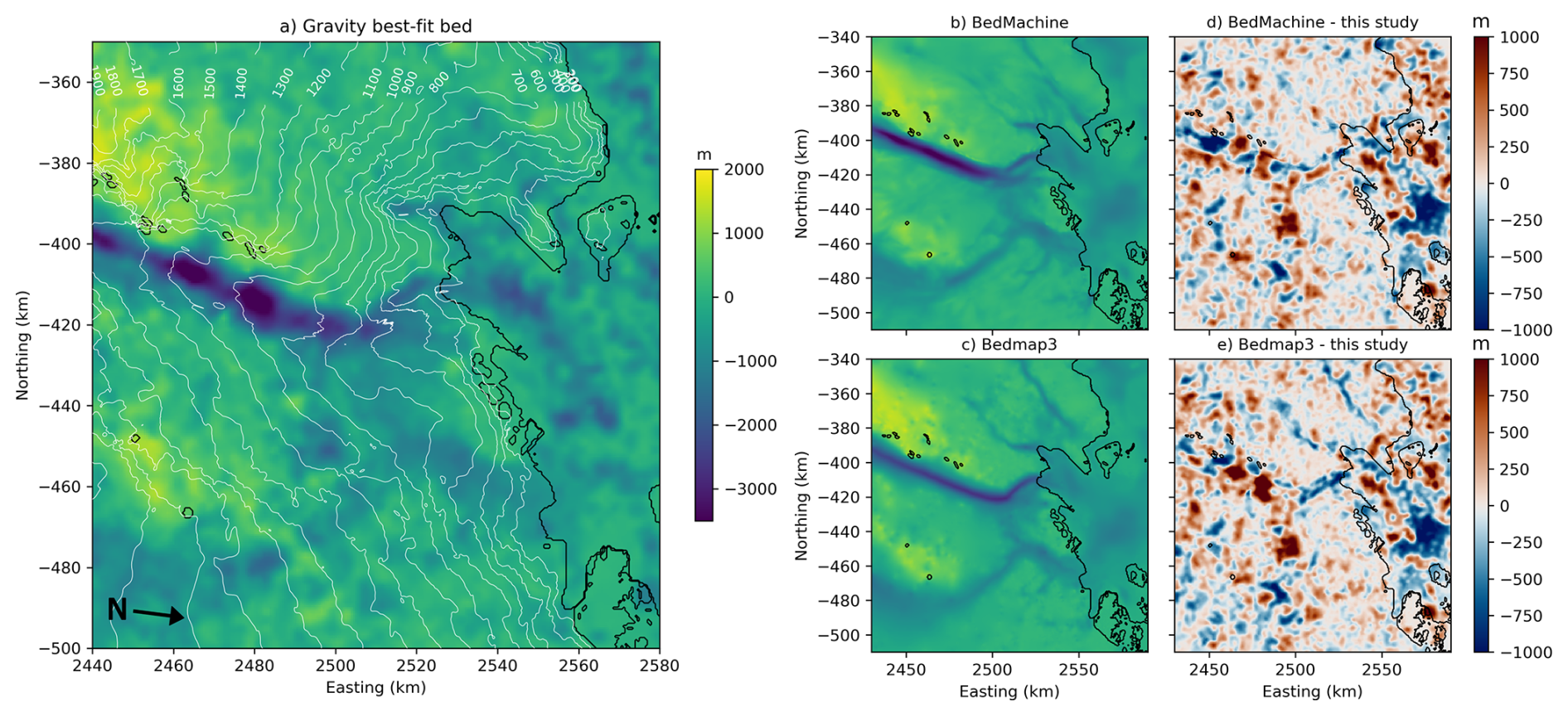
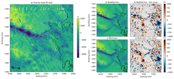
Figure 6 (a) Best-fit subglacial bed elevation in the Denman Glacier region (m, WGS84). White iso lines indicate ice surface height from REMA2 (Howat et al., 2022). (b–c) Bed topography from BedMachine and Bedmap3 for the study region. (d–e) Difference between our best-fit bed reconstruction and BedMachine (Morlighem et al., 2020) (d) and Bedmap3 (Pritchard et al., 2025) (e). Black contours show the ice shelf extent and ice-free land boundaries derived from BedMachine v3.

Figure 6a shows the best-fit bed realization obtained from the gravity inversion. The recovered topography preserves all major structural features observed in the regional setting, including the deep trough running south–north across the domain and the pronounced bed highs along the western margin. The solution exhibits coherent large-scale morphology while also capturing smaller-scale variability consistent with the gravity data constraints. Overlain surface-elevation (Howat et al., 2022) contours illustrate the relationship between the inferred bed and the overlying ice geometry: steep surface gradients generally coincide with deep or rapidly varying bed features, whereas smoother surface topography overlies more gradually varying bed structures. As expected for fast-flowing glacier systems, the deepest parts of the subglacial trough correspond to widely spaced surface contours, indicating relatively low surface slopes. In contrast, steeper surface gradients tend to occur where the bed shoals or where subglacial highs obstruct flow. A notable feature in the surface-elevation contours over the central trough is that neighbouring contour lines locally bend in opposite directions, aligning with the shape of the underlying bed depression. This pattern indicates that the inferred subglacial low is dynamically consistent with the overlying ice-surface morphology. Overall, the best-fit bed provides a physically plausible representation of the subglacial landscape.

Figure 6b–e show the comparison between our gravity-derived bed elevations and the BedMachine and Bedmap3 compilations. Both BedMachine and Bedmap3 depict the main trunk of the trough as a single, continuous, elongated depression. BedMachine shows a slightly sharper and deeper trough expression than Bedmap3. In contrast, the gravity-derived reconstruction shows substantial deviations from both products. The difference fields reveal a pronounced short-wavelength pattern not present in the smoothed and interpolated reference topographies. Instead of a single, uniform deep trough, our solution suggests a more rugged and compartmentalised bed morphology, with multiple depressions and pockets of varying depth rather than one continuous channel. Relative to BedMachine (Fig. 6b and d), our model predicts generally deeper pockets (red areas) along the central trough axis, especially in its mid-section, and shallower terrain (blue areas) upstream, indicating internal structure not expressed in BedMachine. Relative to Bedmap3 (Fig. 6c and e), the gravity-derived field exhibits larger positive deviations upstream and stronger negative deviations toward the downstream coastal margin, again reflecting a more variable bed than the broad, smoothed trough depicted in Bedmap3. Notably, our reconstruction also reveals a deep, trough-like structure beneath the ice shelf as a continuation of the inland trough, which is not resolved in either BedMachine or Bedmap3. Overall, the gravity-based reconstruction suggests a more heterogeneous subglacial landscape, characterised by localised depressions and subdued ridges, which are muted or absent in current continent-scale compilations.

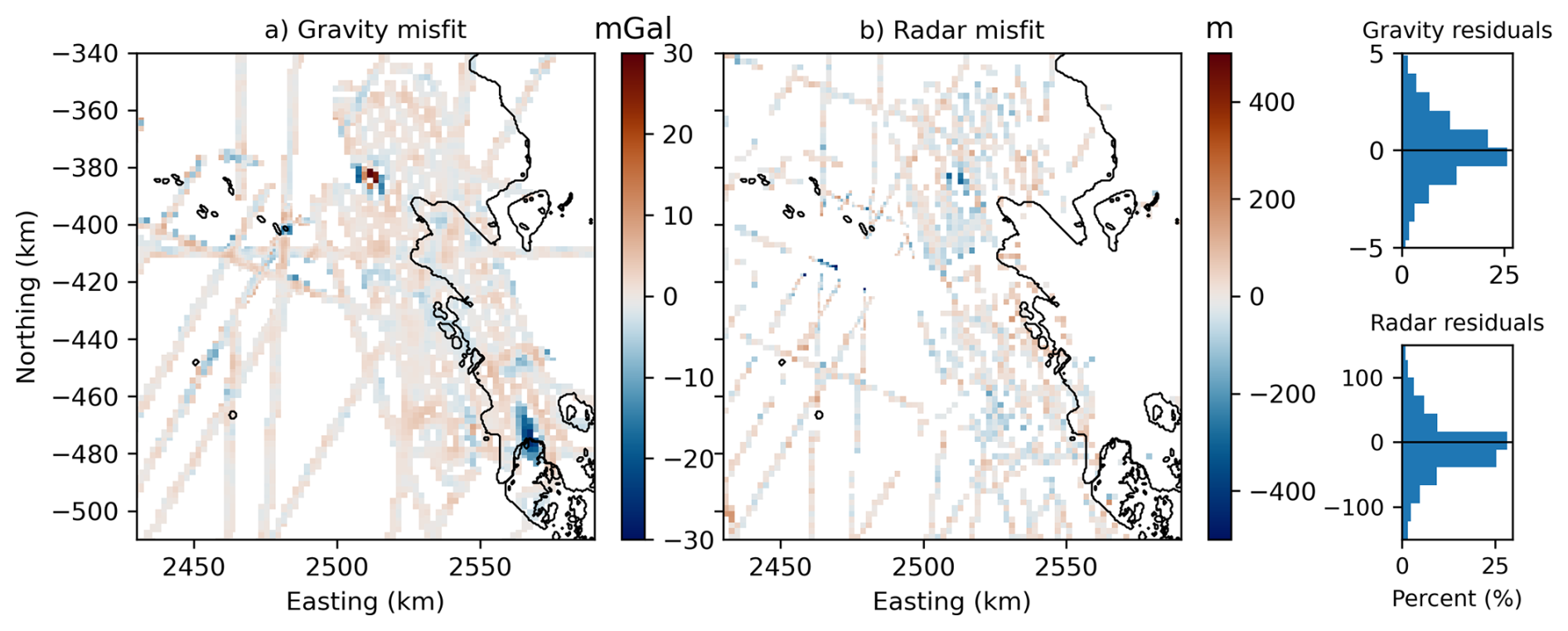
Figure 7 (a) Gravity misfit for the best-fitting realization (target − modeled). (b) Radar misfit for the best-fitting realization (target − modeled). Histograms show the distribution of gravity and radar residuals, expressed as the percentage of all grid cells. Black contours show the ice shelf extent and ice-free land boundaries derived from BedMachine v3.

Observed minus forward-modeled gravity for the best-fit-gravity (Fig. 7a) shows that residuals are predominantly small (∼ ±10 mGal), with a mean absolute error (MAE) of 1.6 mGal and a RMSE of 3.0 mGal. Isolated misfit clusters approach values ±50 mGal. The absence of large-scale, coherent residual patterns indicates that the bed captures the main gravity signal in the area. The radar misfit map (Fig. 7b) shows that the inversion reproduces radar-derived bed elevations well across most of the domain. Misfits are generally small, with most values within ±100 m, reflecting the strong influence of radar constraints.

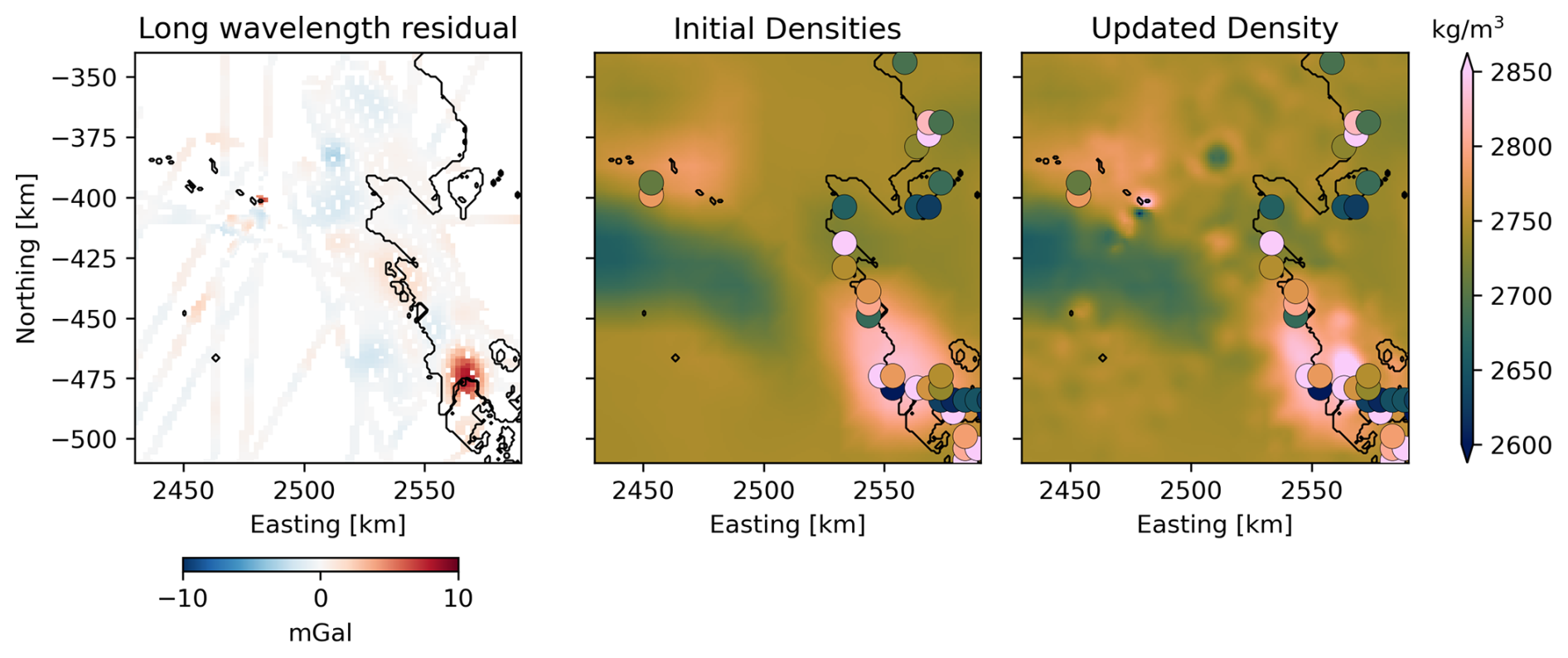
Figure 8 Rock density field before and after gravity‐guided update. (a) Long-wavelength residual at measurement locations, after removing the short-wavelength component (see Sect. 3.3). (b) Initial rock densities inferred from gravity and magnetic joint inversion by Lösing et al. (2025b). (c) Updated densities after damped least-squares inversion of the long-wavelength gravity residual. Colored circles show binned rock-sample densities (Lösing et al., 2025a). Black contours show the ice shelf extent and ice-free land boundaries derived from BedMachine v3.

Figure 8 illustrates the long-wavelength part of the gravity residual (Fig. 7a) used for the density update (Sect. 3.3), the prior rock-density field, and the updated density model after inversion. The strongest positive residual occurs in the northeastern sector of the Denman Glacier region, indicating a possible mass deficit in the prior model, whereas weaker negative residuals appear toward the west, suggesting locally overestimated densities. The density update shifts the model toward higher densities in the northeast, reducing the strong positive residual, and lowers densities in the central-western part of the area. Short-wavelength track artefacts are suppressed by Gaussian smoothing, isolating only the spatially coherent residual signal used in the update. In-situ rock sample densities overlain as coloured circles span roughly 2300–3100 kg m⁻³ and provide a reference for assessing the plausibility of both the initial and updated models.

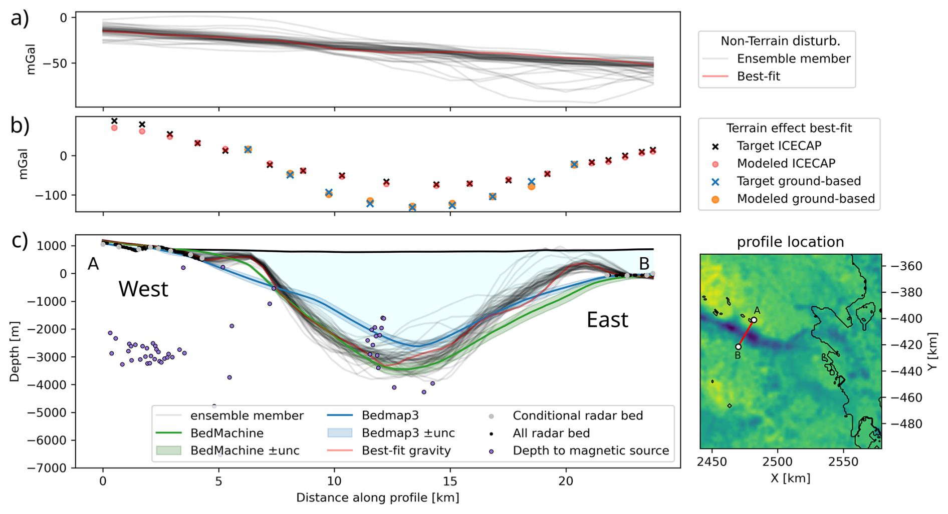
Figure 9 Along‐transect cross‐section A–B of the Denman Glacier trough. (a) Non-terrain gravity disturbances (mGal). (c) Comparison of bedrock interface estimates, showing radar-derived bed picks (black dots), conditional radar points (silver dots), ensemble results (grey lines), and the best‐fit inverted bed (light red). For reference, Bedmap3 ± uncertainty (blue ribbon), BedMachine ± uncertainty (dark green ribbon), and DMS estimates (purple dots) are included alongside the ice surface (black).

Figure 9 shows a cross-sectional comparison of the gravity-derived bed ensemble, published bed compilations (BedMachine; Morlighem et al., 2020; and Bedmap3; Pritchard et al., 2025), radar bed picks, and the depth to the magnetic basement along the ICECAP flight line ASB/JKB2c/Y11b (Fig. 1a).

The ensemble of accepted gravity solutions (grey lines) spans a narrow range near the trough margin at both ends of the profile but diverges strongly within the deep central trough. This widening reflects the lack of radar bed constraints across the trough and the poorly known geology, leading to greater non-uniqueness in the gravity-derived solutions. The best-fit gravity bed (light red) follows the overall morphology of the trough, producing a smooth and dynamically plausible shape while remaining well within the ensemble variability. Radar picks along the transect agree closely with the gravity best-fit bed at both margins.

Both BedMachine (green) and Bedmap3 (blue) differ from the gravity-derived solution. Bedmap3 predicts a broader and shallower depression, whereas BedMachine yields a steeper and more V-shaped form. Their respective uncertainty envelopes (light green and light blue) encompass part of the ensemble range but do not fully capture the total spread produced by the gravity inversion. This indicates that gravity introduces additional constraints reflecting the integrated subsurface mass distribution, thereby informing trough shape, depth, and geological structure in ways that are not fully represented in the existing compilations.

In the west, DMS estimates (purple circles) lie several kilometers beneath the radar-derived bed, suggesting that the magnetic sources are located well below the ice–bed interface. However, a few isolated DMS points coincide with the western flank of the various topographic models, which may indicate the presence of a strong magnetic source at depth, accompanied by weaker signals originating from the ice–bed interface. In the central part of the profile, a cluster of DMS points displays a subvertical alignment suggesting a steeply dipping, magnetically susceptible fault zone. This structure likely marks a lithological boundary, separating non-magnetic sedimentary units to the east from magnetic crystalline basement to the west. The Denman Glacier trough appears to exploit this structural weakness. Notably, this interpreted contact lies within 1–2 km of the proposed location of the Scott Fault (Manassero et al., 2026), consistent with previous geophysical and geological interpretations (Maritati et al., 2016; Aitken et al., 2014; Aitken and Urosevic, 2021). The eastern side is characterized by more subdued magnetic responses, likely reflecting sedimentary or metasedimentary units. However, the lack of DMS solutions in the east may alternatively be due to deeper magnetic sources, suboptimal parameter settings (Sect. 3.4), or reduced data quality.

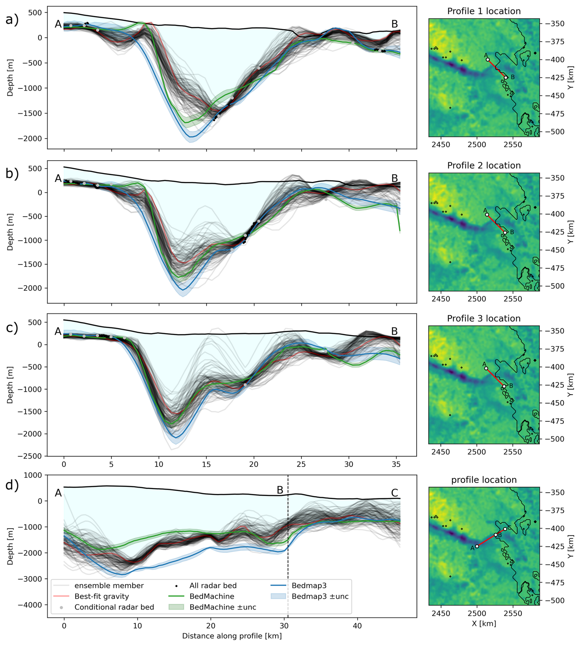
Figure 10 (a–d) Left panels: bed elevation along profiles in the grounding zone. Grey lines show the full ensemble of bed solutions; the thick black line shows the ice surface from BedMachine. Red dots mark gridded radar bed measurements used to condition the inversion, while small black dots show all available radar bed picks. The green lines show BedMachine topography with its uncertainty envelope, and the blue lines show Bedmap3 topography with its associated uncertainty. Coastlines are shown in black. Profiles (a)–(c) cross the main deep trough, while profile (d) follows a longer transect extending downstream towards the marine outlet.

Figure 10 presents four transects (a–d) across the study region, comparing the gravity-derived ensemble of admissible bed realizations with BedMachine, Bedmap3, and radar-derived bed elevations. Profiles (a)–(c) intersect the grounding zone of the subglacial trough system, sampling progressively inland sections of the topography, whereas profile (d) runs approximately along-trough and perpendicular to the other profiles, providing complementary constraints on trough geometry. Across all profiles, the ensemble members converge tightly where radar observations constrain the bed, yet diverge substantially within the deep trough interior where radar coverage is absent. In the three upstream profiles (Fig. 10a–c), the best-fit gravity-derived bed consistently reveals a steeper, more sharply defined trough geometry, yet generally shallower than either BedMachine or Bedmap3. These differences suggest structural or geological controls that are not represented in the interpolation-based surfaces of the existing compilations. The gravity ensemble also indicates the presence of a potential topographic high within the central portion of the profiles. This feature may reflect a subdued bedrock ridge that partitions the trough into two segments, an internal structure that appears less pronounced in BedMachine and Bedmap3.

Profile (d) displays a longer transect (A–B–C) crossing the grounding zone and capturing the downstream continuation of the trough. Compared with the best-fit gravity solution, BedMachine aligns reasonably well with the intermediate basin but is smoother and shallower toward point A, while Bedmap3 predicts a markedly deeper structure. The gravity best-fit bed consistently occupies the space between these two endmember interpretations. A notable feature is the change in trough geometry across the dashed marker at B, marking the transition from the inland region to the offshore bathymetric domain beneath the ice shelf, where no radar data are available. Across this boundary, the ensemble suggests a shift from a deep, steep-sided continental basin to a more subdued offshore morphology, although the latter remains comparatively unconstrained due to the absence of radar observations.

5 Discussion

5.1 Gravity non-uniqueness

Gravity inversions are inherently non-unique: an infinite family of density–depth combinations can reproduce the same anomaly, and solutions are further blurred by measurement errors, terrain corrections, and upward continuation that suppresses short wavelengths (e.g. Blakely, 1996; Telford et al., 1990). This ambiguity is especially acute beneath thick ice where direct constraints are sparse, as in Denman Glacier (Tankersley et al., 2025).

To mitigate this, we used SGS to generate an ensemble of plausible terrain effects, exploring a range of realizations rather than relying on a single deterministic solution. This incorporates structural uncertainty, reduces overfitting bias, and highlights features that persist across realizations. In practice, however, when a strong regional, non-terrain disturbance is present, mis-estimation of that field dominates the error (Field et al., 2026). In such cases, adding well-placed constraints is more effective than modest noise reductions or additional re-flights (Tankersley et al., 2025). In our inversion, Monte Carlo uncertainty maps consistently flag high-error zones, guiding where new constraints or targeted (re-)flights will most improve the solution.

Along the Denman trough, steep flanks introduce trade-offs between density contrast and interface geometry that can translate into kilometer-scale variations in inferred depth. With the one-layer ice-bedrock contrast formulation used here, the modeled gravity low can absorb both residual terrain effect and genuine geological signal; it should therefore be viewed as a composite response rather than a uniquely resolved basement surface. Where trough geology departs from surrounding radar-constrained regions, the inversion lacks leverage to isolate the geological component, and a unique depth solution is not expected. Additional independent constraints will be required to separate these contributions. A longer ground-based gravity profile with overlap into areas of existing radar bed picks would help constrain the geological component more robustly. Incorporating magnetotelluric (Manassero et al., 2026) and/or seismic information would help refining the estimates and deepen our understanding of the subsurface geology.

The joint misfit combines gravity and radar constraints through prescribed uncertainties (σ_g and σ_h) and a dimensionless weighting factor μ (Sect. 3.2). In our baseline formulation we set μ=1, ensuring that the two datasets contribute to the likelihood strictly according to their assumed uncertainties. This allows the inversion to converge toward bed geometries that are statistically consistent with the stated error structure, without introducing additional subjective weighting. Because gravity and radar misfits therefore enter the likelihood on equal footing per unit of normalised misfit, any mis-specification of σ_g or σ_h would implicitly shift the balance between the datasets. Our approach reflects a deliberate choice to let the inferred geometry be governed by the reported uncertainties rather than by manual tuning.

5.2 Denman Glacier Trough Geometry

The sensitivity of the final results to the initial condition is low. First, we re-draw the Gaussian perturbation for every MCMC realization, ensuring that the ensemble does not inherit structure from any single starting model. Second, the magnitude of the perturbation is selected to be in a similar range of systematic differences between BedMachine and Bedmap3 in this region, preventing the sampler from being biased toward either compilation. As a consequence, the inversion explores a broad portion of the model space, and the posterior ensemble is dominated by the gravitational misfit rather than by the specific choice of initial bed geometry. This yields solutions that are effectively independent of the initial condition while still allowing the method to converge toward geologically and dynamically plausible structures.

The geometry revealed by the gravity-derived beds reinforces the susceptibility of Denman Glacier to Marine Ice Sheet Instability (MISI). In a marine setting, grounding line stability is strongly dependent on the underlying bed geometry (Weertman, 1974; Schoof, 2007). As a result, if the grounding line retreats onto a deeper, inland-sloping bed, buoyancy forces increase while ice flow accelerates, promoting a positive feedback loop of unstable retreat. The Denman Trough's steep and potentially retrograde geometry (Fig. 10) is therefore of particular concern, as such configurations can promote MISI under certain combinations of atmospheric forcing and basal conditions (e.g., Sergienko and Wingham, 2024). However, along- and across-trough ridges (pinning points) could temporarily stabilize the grounding line by increasing basal/side drag and promoting local back-stress, once these highs are passed, instability can resume. While the presence or absence of MISI cannot be inferred from geometry alone, our results provide physically realistic basal boundary conditions that can be tested within ice sheet models to assess the susceptibility of this sector to future retreat and its possible contribution to long-term mass loss from the East Antarctic Ice Sheet.

Our probabilistic inversion differs from Shao et al. (2026) in both, data basis and physical assumptions. Rather than relying on mass conservation and ice-dynamical constraints, our method uses gravity. This produces a complementary estimate of bed geometry that reflects the integrated mass distribution beneath the ice sheet, only weakly constrained by ice flow dynamics. The two approaches therefore illuminate different aspects of the system. Shao et al. (2026) quantify how much bed geometry can vary while remaining dynamically consistent with present-day ice flow, but it inherits limitations where surface velocity gradients are small. Our gravity-based ensemble, by contrast, is unaffected by ice dynamics and instead reflects the deeper mass distribution. As a result, it tends to predict more compartmentalised, rugged trough geometries, including multiple local depressions within the broader Denman basin. These differences suggest that the dynamical constraint of mass conservation alone does not fully capture the complexity of the subglacial landscape in this region, and that complementary geophysical constraints such as gravity are essential for identifying plausible structural configurations. Taken together, their combined perspectives emphasize the need for ensemble-based modeling that incorporates both ice-dynamic and solid-Earth constraints when assessing basin geometry, grounding line sensitivity, and future retreat scenarios.

5.3 Depth of magnetic sources

While Euler deconvolution provides a rapid estimate of magnetic source depths, it has several limitations. The method is sensitive to the magnitude of susceptibility contrasts; weakly magnetized rocks may yield weak anomalies that are difficult to interpret. Depth estimates depend critically on the assumed structural index, and misinterpretations can arise if the true source geometry differs from the model. In addition, the method amplifies data noise through the calculation of spatial derivatives, and its resolution is inherently limited by the flight altitude and the depth to magnetic sources. Remanent magnetization and the choice of window size further influence solution stability and accuracy, particularly in regions of deep or complex geology such as the Denman Trough.

The ICECAP magnetic data were acquired at an average flight height of approximately 2 km relative to the WGS84 ellipsoid. Over the Denman region, where the ice surface itself lies roughly 1–2 km above the ellipsoid, this corresponds to an effective height of approximately 0.5–1 km above the ice surface. Consequently, the minimum resolvable magnetic wavelengths range from about 1–3 km (Telford et al., 1990). At suggested trough depths of 3–6 km beneath the ice surface, the source-to-sensor distances imply that only magnetic anomalies with wavelengths larger than approximately 6–18 km are well resolved, favoring the detection of broader geometries rather than fine-scale basement features (Fig. B1).

6 Conclusions

In this study, we present an ensemble of gravity-derived bed topography realizations for the Denman Glacier region, revealing a more complex and dynamically important trough geometry than represented in existing radar-interpolated and mass conservation products. By integrating ensemble-based gravity inversion with radar picks and depth to magnetic source estimates, we show that Denman Glacier overlies a deeply incised, asymmetrical, and internally segmented trough system. The depth to magnetic source solutions further support a tectonically influenced structure with contrasting lithologies across the trough flanks, crystalline basement to the west and weaker, sedimentary signatures to the east.

Across the cross-trough profiles near the grounding line, the best-fit gravity bed consistently falls between BedMachine and Bedmap3 and reveals more pronounced relief than either compilation. Near the grounding line, the ensemble also indicates a potentially subdued bedrock high dividing the trough into two connected basins and suggests a continued channel beneath the ice shelf, features not captured in current Antarctic bed products.

Together, the steep flanks, retrograde inland slope, strong asymmetry, and limited stabilizing topographic highs point to a bed geometry that could enhance Denman Glacier's susceptibility to Marine Ice Sheet Instability. The discrepancies between gravity-constrained geometry and widely used compilations highlight that many ice sheet models may currently rely on overly smoothed bed representations, potentially underestimating grounding line sensitivity. These findings underscore the importance of incorporating geophysical inversion results into future Antarctic bed mapping efforts, especially for fast-flowing outlet glaciers where modest changes in bed geometry can have major implications for ice dynamics.

In summary, this work provides new constraints on the morphology and geological context of the Denman trough, identifies features relevant for grounding line stability, and delivers a revised bed representation with uncertainties that is directly applicable to ice-flow modeling and assessments of future retreat risk.

Appendix A: Data

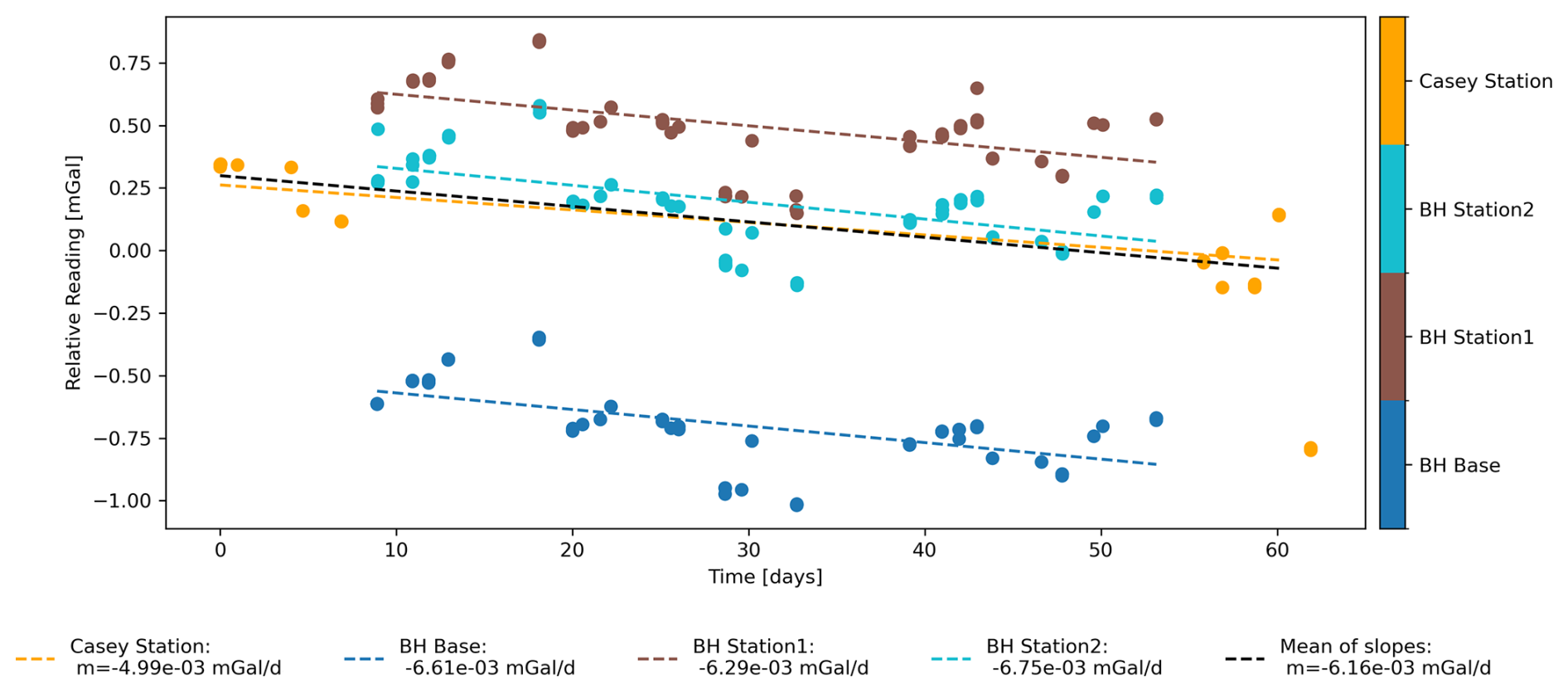
Figure A1 Relative gravity readings (subtracted mean) versus elapsed time. Colored points show individual measurements from each site (see colorbar: Casey Station in orange; BH (Bunger Hills) Base (Lon: 100.6048, Lat: −66.2496, height: 10.062 m), BH Station 1 (Lon: 100.6044, Lat: −66.2504, height: 6.125 m), and BH Station 2 (Lon: 100.6068, Lat: −66.2509, height: 6.318 m) in blue/brown/light blue, respectively). Dashed colored lines are least-squares fits to each site; legend entries report the fitted slope (in mGal d⁻¹). The black dashed line is the average slope across all series.

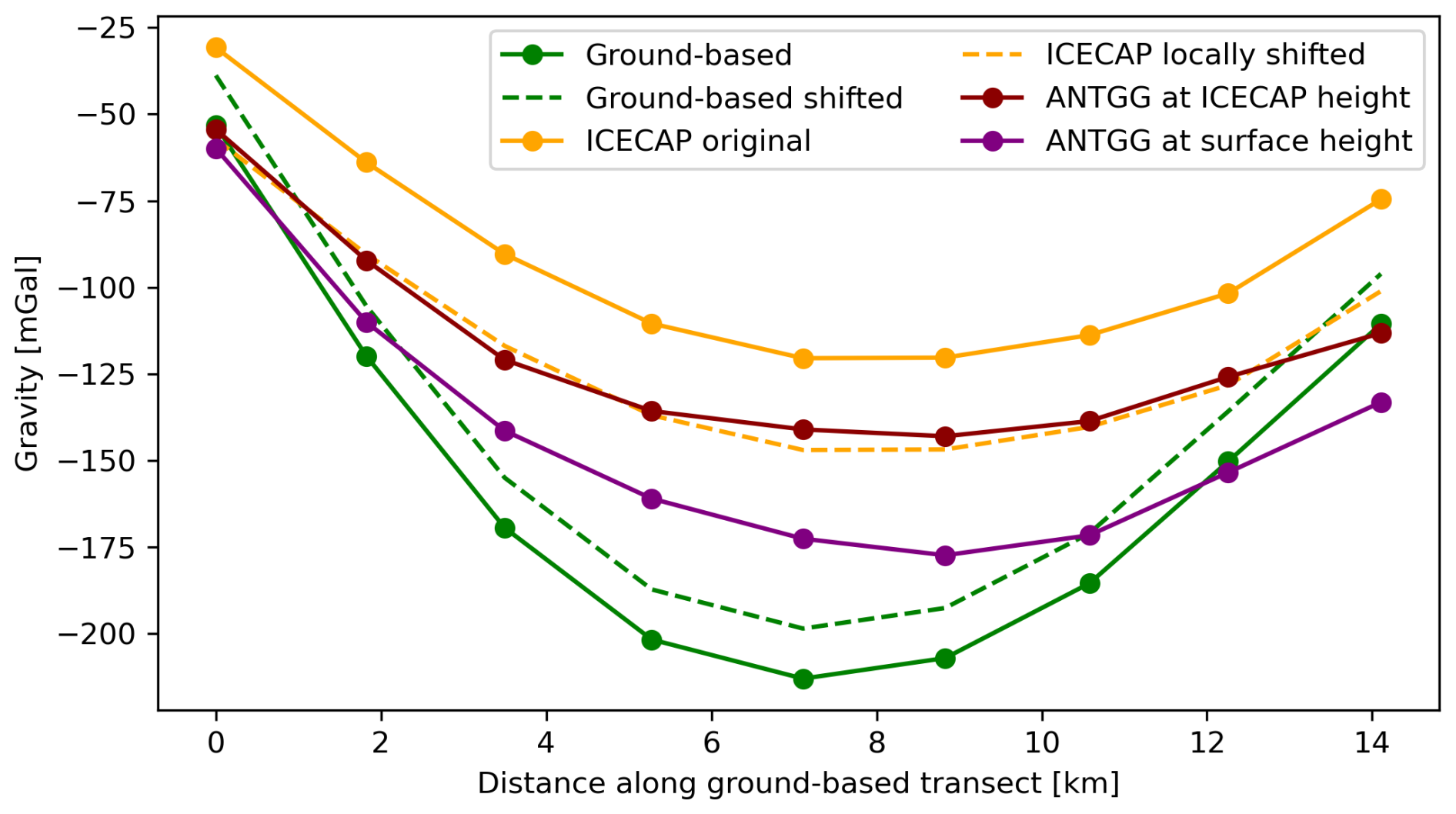
Figure A2 Ground-based gravity data compared with airborne ICECAP measurements and the AntGG2021 reference field at the surface (Scheinert et al., 2024) along the Denman transect. Solid lines indicate original data, while dashed lines show the data after applying a shift based on AntGG2021 (details in Sect. 2.3). All datasets are plotted against distance along the ground-based transect (Fig. 1a).

Appendix B: Depth to Magnetic Source

Airborne magnetic data from the ICECAP project (Blankenship et al., 2011; Roberts et al., 2018), reprocessed by Aitken et al. (2020) to obtain Total Magnetic Intensity (TMI), are available across the Denman Glacier region and are upward continued to a common height of 2 km. These data can be used to estimate the depth to magnetic source (DMS, Fig. B1), which is the boundary between non-magnetic sediments and magnetically susceptible crystalline basement, and investigate subsurface structures and lithological boundaries across the study area.

We estimate the depth to the magnetic basement beneath the subglacial trough using Euler deconvolution, following the method of Melo and Barbosa (2020). This approach solves Euler's homogeneity equation, which relates the local magnetic field and its spatial gradients to the position of a magnetic source:

$$(x-x_{\mathrm{0}}){\displaystyle \frac{\partial T}{\partial x}}+(y-y_{\mathrm{0}}){\displaystyle \frac{\partial T}{\partial y}}+(z-z_{\mathrm{0}}){\displaystyle \frac{\partial T}{\partial z}}=-NT$$

where $(x_{\mathrm{0}},y_{\mathrm{0}},z_{\mathrm{0}})$ is the estimated source location, T is the total magnetic anomaly, and N is the structural index (SI), a scalar that depends on the geometry of the source. In this study, we use N=0, appropriate for sharp vertical contacts, which is appropriate for the expected sharp boundary between non-magnetic overburden and magnetized basement at the trough flanks. We also tested using N=1, which is appropriate for thin, vertical sheet-like (dike) bodies. Finally, we adopt N=0 because it more consistent with the regional geology, where sharp lithological boundaries are expected rather than discrete, sheet-like intrusions. In our experiments, solutions with N=0 also yielded geologically coherent and spatially consistent results.

Spatial derivatives of the anomaly field were computed in the frequency domain using fast Fourier transforms with edge-value padding to minimize boundary artifacts. Euler deconvolution was then applied over a moving window across the anomaly grid, with a linear system solved at each window location to estimate the source depth and lateral position. To enhance solution reliability and reduce spurious estimates, All solutions are ranked based on the standard deviation of the vertical derivative $\partial T/\partial z$ within each window. Only a fixed proportion (here the top 10 %) of the highest ranked solutions is retained. This filtering strategy improves the localization of coherent source bodies and suppresses noisy results.

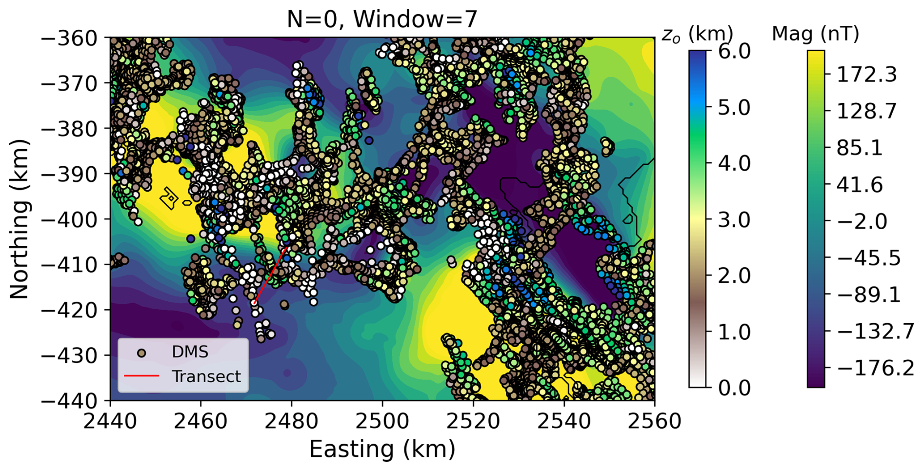
Figure B1 Euler deconvolution solution depths N=0 calculated with a structural index of N=0 and a window size of 7, overlain on the magnetic data grid. Colored circles represent individual depth to magnetic source solutions. The red line marks the location of the ground-based gravity transect.

Euler deconvolution solves for source locations within moving data windows. Window size determines how many points enter each local inversion and the scale over which derivatives are evaluated. Small windows improve resolution of shallow, fine-scale structures but are noise-prone, large windows yield smoother, more stable results that can obscure detail or blend geologically disparate areas. We tested multiple window sizes (3, 5, 7, and 9 data points) within a ∼ 500 × 500 m grid (median along-flight line spacing) to evaluate the stability and resolution of the depth solutions. We find that a window size of 7 provides an effective balance between stability and spatial resolution and is appropriate for moderately deep sources (e.g., Reid et al., 1990), consistent with the dataset's resolution and anticipated feature scales. A larger window of 9 produces comparable solutions, differing only by about 500 m greater depth in the west and no change at mid-trough.

Appendix C: Results

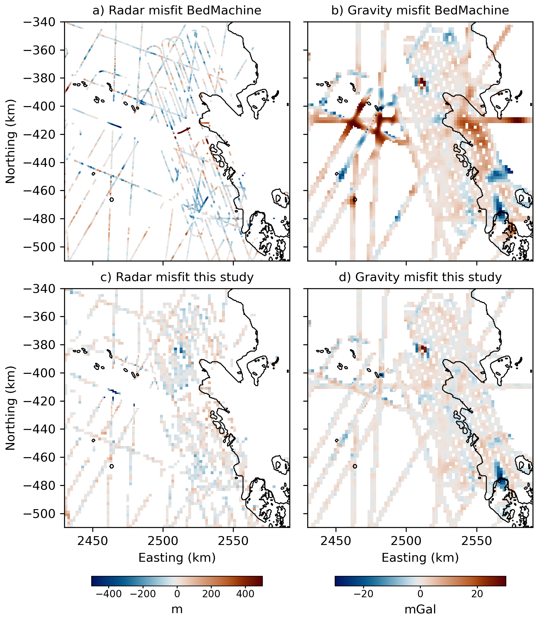
Figure C1 Comparison of radar- and gravity-derived misfits between the BedMachine bed topography (Morlighem et al., 2020) and the updated inversion presented in this study. (a) Misfit between BedMachine topography and radar observations (modeled − observed), and (b) differences between terrain effects (b) (BedMachine − best-fit target of this study). (c) Misfit between best-fit bed estimate obtained in this study and radar observations (modeled − observed), and (d) differences between terrain effects (modelled − best-fit target of this study). In all panels, black contours show the ice shelf extent and ice-free land boundaries derived from BedMachine v3.