Field-validated imaging of decadal and seasonal changes in permafrost bedrock using quantitative electrical resistivity tomography (Zugspitze, Germany/Austria)

Ongoing permafrost degradation in alpine regions requires monitoring methods that accurately decipher spatial and temporal dynamics. Electrical resistivity tomography (ERT) is widely applied in bedrock permafrost, yet its outputs are often interpreted only qualitatively. Quantitative evaluation of ERT results, however, is crucial for improving process understanding and enhancing predictions of permafrost-related slope instability. In this study, we present a 17-year monitoring of permafrost rock slopes on Mount Zugspitze (Germany/Austria) with monthly ERT campaigns. ERT data are combined with rock temperatures at four depths to establish field-based temperature–resistivity calibrations and to validate existing laboratory-derived relations. Both approaches agree well in the freezing range; however, field calibrations tend to yield higher resistivities at subzero temperatures and reveal substantial spatial heterogeneity. Incorporating reciprocal measurements refines the existing error model, increases image resolution, and improves the identification of subsurface features. Over 10 years, the measured rock temperature increased by 1 °C, accompanied by a 25 % decrease in resistivity. The permanently frozen surface decreased by 40 %, with degradation rates up to −4.2 kΩm yr⁻¹. Extrapolating these trends would result in the loss of 65 % of permafrost within a decade. Thermal forcing controls the degradation; however, the observed conditions and projected increases in heatwaves suggest that newly unfrozen and connected fracture networks will enhance advective heat transport. This heat shortcut is expected to accelerate permafrost warming and thawing, thereby increasing the risk of slope instability. With these results, we demonstrate that ERT monitoring can yield high-quality quantitative insights into long-term permafrost evolution and effectively track bedrock permafrost degradation across both decadal and seasonal timescales.

1 Introduction

In the last few decades, air temperatures have reached unprecedented record values during repeated summer heatwaves, with consequences also underground. Warming of frozen ground is well documented at all latitudes and altitudes worldwide (Biskaborn et al., 2019; Smith et al., 2022; Gruber et al., 2017; Masiokas et al., 2020; Aalto et al., 2018) with European mountain permafrost warming about 0.4 °C in the last 20 years (Etzelmüller et al., 2020; Noetzli et al., 2024). This degradation is projected to continue in response to climate change, but its magnitude and timing are uncertain, as the thermal response appears to be site-specific (Smith et al., 2022). In fact, it depends on material, topography, surface characteristics, slope histories, permafrost type (warm vs. cold), and, most specifically, ice content (Magnin et al., 2017; Haberkorn et al., 2021; Deline et al., 2021). Ice-poor bedrock permafrost, close to 0 °C, has recently experienced the strongest warming (Magnin et al., 2023). If ice is present, permafrost degradation appears to be non-linear due to latent heat effects (Hauck and Hilbich, 2024). Degrading permafrost has demonstrably increased slope instability (Krautblatter et al., 2013; Mamot et al., 2021), as shown by recent rockfalls, rock glacier acceleration, debris flows, and other cascading phenomena (Huggel et al., 2012; Phillips et al., 2017; Walter et al., 2020; Deline et al., 2021). Therefore, it needs to be closely monitored.

Geophysics can support these investigations with deep and spatially extensive insights (Vonder Muehll et al., 2001). Electrical Resistivity Tomography (ERT) clearly detects permafrost due to the large resistivity contrasts between frozen and unfrozen conditions (Tsytovlch and Sumgin, 1937; Muller, 1947; Parkhomenko, 1967). Focusing on mountain environments, ERT was introduced in the early 2000s (Vonder Muehll et al., 2000; Hauck, 2001). It quickly evolved into 2D surveys (Hauck and Vonder Muehll, 2003; Kneisel, 2004; Marescot et al., 2003) with Krautblatter and Hauck (2007) first applying it to bedrock permafrost, followed by 3D surveys (e.g., Rödder and Kneisel, 2012; Duvillard et al., 2018; Scandroglio et al., 2021), and cross-borehole measurements (Phillips et al., 2023; Bast et al., 2024). Repetition of measurements, i.e., time-lapse ERT, proved its capability to monitor permafrost changes (Hilbich et al., 2008; Krautblatter et al., 2010; Pogliotti et al., 2015; Scandroglio et al., 2021). Fundamental for reproducibility is a robust setup (Kneisel et al., 2014), but only recently have standard procedures been suggested (Herring et al., 2023). The majority of time-lapse studies are composed of one single measurement per year at the end of summer for permafrost detection (e.g., Kellerer-Pirklbauer and Eulenstein, 2023; Pavoni et al., 2023; Cathala et al., 2024) and the repetition of surveys accounts only for 20 % of the studies (Herring et al., 2023). Most of these were single repetitions (e.g., Magnin et al., 2015; Buckel et al., 2023), some monitoring occurred at irregular time intervals (Scandroglio et al., 2021; Etzelmüller et al., 2023; Noetzli and Pellet, 2024), and only a few sites were regularly monitored (Mollaret et al., 2019; Morard et al., 2024). Although knowledge of the minimum permafrost extension at the end of summer is sufficient for most sites, hazardous locations require a higher temporal resolution to interpret site-specific, complex hydrothermal dynamics at depth (Krautblatter et al., 2010; Kneisel et al., 2014; Offer et al., 2025). This enables the evaluation of rock instabilities (Keuschnig et al., 2015; Etzelmüller et al., 2022; Cathala et al., 2024) to inform the development of effective geotechnical solutions and appropriate risk-reduction strategies (Bommer et al., 2009; Deline et al., 2021). Automated time-lapse ERT can provide high temporal resolution (Kneisel et al., 2014; Doetsch et al., 2015). However, the analyses published so far are limited to 2 years or have significant gaps due to frequent technical failures (Hilbich et al., 2011; Supper et al., 2014; Keuschnig et al., 2017). Therefore, automated ERT has rarely been used to examine long-term trends in permafrost change (Herring et al., 2023). The only known work presenting continuous decadal data at monthly resolution is by Mollaret et al. (2019) at the Schilthorn (CH).

Quantification of permafrost changes can be obtained by calculating the average resistivity of the whole model (Hilbich et al., 2008) or only of the area of interest (Kneisel et al., 2014). Quantitatively translating resistivity values into temperatures is a non-trivial task, as many factors influence the measurements (Krautblatter et al., 2010). Laboratory calibration of bedrock samples was first introduced by Krautblatter et al. (2010) and subsequently employed in several studies to enhance the interpretation of geophysical data in permafrost environments (e.g., Magnin et al., 2015; Etzelmüller et al., 2022; Scandroglio et al., 2021), although without quantitative field validation. ERT validation is possible with borehole data (Vonder Muehll et al., 2000; Lewkowicz et al., 2011; Doetsch et al., 2015; Mollaret et al., 2019; Farzamian et al., 2020) to constrain the interpretation of the results. While many studies report both borehole temperature data and ERT measurements, a direct comparison and validation between the two is rare in the literature. Only in recent studies, shallow borehole data have been used to calibrate automated ERT datasets: e.g., in arctic sediments (Cimpoiasu et al., 2024, 2025). Further, to our knowledge, no study has validated laboratory-based calibrations in the field.

Here, we present the first field-validated long-term temperature-resistivity monitoring over more than 10 years in bedrock permafrost. This database originates from a high-alpine location (Mount Zugspitze, Germany/Austria, 2800 m a.s.l.). It is unique due to its monthly resolution, the location of the electrodes in the permafrost core rather than on the surface, and the high-quality results achieved through manual measurements. Results are compared with those of Krautblatter et al. (2010) to validate the methods and investigate the effects of climate change. This study aims to determine whether ERT monitoring can provide robust quantitative insights into long-term permafrost evolution and effectively capture bedrock permafrost degradation over both decadal and seasonal timescales. This overarching objective is explored through four key quantitative research questions:

1. How reliable is laboratory calibration, and is it consistent with field calibration and observations?

2. Do enhanced error models improve the reconnaissance of thermal processes in bedrock?

3. What long-term trends and seasonal signals of permafrost degradation can be effectively captured with monthly resolution?

4. At the Zugspitze, can we quantify permafrost extent, its degradation over a decade, and anticipate its future development?

2 Material and Methods

2.1 Field site

Measurements took place in the Kammstollen, a private tunnel beneath the E-W oriented ridge of Zugspitze (2962 m a.s.l., Fig. 1a–b), located at the German-Austrian border. This mountain is part of the Northern Calcareous Alps, and its summit is composed of Upper Triassic carbonate rocks, mainly massive limestones of the Wetterstein Formation (Miller, 1962). The thick-bedded, locally dolomitized rocks commonly exhibit fracturing and karstification due to dissolution, which are frequent and well documented on the nearby Plateau (Wrobel, 1980; Wetzel, 2004). Minor dolomite and occasional marl intercalations reflect depositional variability, while brecciated zones up to 1 m thickness are present in the summit area (Ulrich and King, 1993). A prominent fault zone extends from the investigation area up to the summit (Hornung and Haas, 2017), but overall, the steep summit cliffs consist of comparatively pure, competent carbonate rocks. The study area is accessible year-round thanks to the infrastructure and logistical support of the research station, Scheefernerhaus (UFS), which is directly connected to the tunnel.

Long-term meteorological records on the summit by the German Meteorological Service (DWD) are available since 1900 (Fig. 1c). Air temperature increased drastically in the last 30 years, with mean temperatures in the last decade (2013–2022) reaching −3.3 °C, which is 1.5 °C warmer than the reference period 1961–1990. Additionally, 2011, 2020, 2022, and 2024 were the warmest years on record. Mean annual precipitation is more than 2500 mm of which 80 % is snowfall, but the steep north walls remain snow-free for most of the winter. The hydrological behavior of clefts at this location has been thoroughly measured for many years and interpreted by Scandroglio et al. (2025).

2.2 State of the cryosphere at the Zugspitze

The earliest records of permafrost on the Zugspitze date to the construction of its infrastructure (AEG, 1931; Körner and Ulrich, 1965; Ulrich and King, 1993). In recent years, 3D modeling has confirmed the possible presence of permafrost on the shaded and steep north side of the SW-NE ridge, which includes the site of this study, beginning at approximately 2350 m a.s.l., but suggests a rather warm permafrost (Noetzli et al., 2006). Based on this modeling, one N-S borehole was drilled in 2007 by the Bavarian Environmental Agency (LfU) about 30 m under the summit to document permafrost presence and evolution under the summit cable car, at a distance of 700 m from our field site (Gallemann et al., 2017, 2021; Wagner et al., 2023). These measurements support the modeling, showing average core temperatures between −1.2 and −0.7 °C, with a warming trend of 0.4 K in the last ten years. Modeling by Gallemann et al. (2017) forecasts the disappearance of this lens by 2070. Krautblatter et al. (2010) conducted the first ERT monitoring in the tunnel in 2007, setting the basis for this study. The tunnel comprises a main tunnel (MT) and a side tunnel (ST). Ice accumulated across the entire ground of the side tunnel and in parts of the main tunnel, reaching a depth of up to 50 cm in some locations. Recently Mamot et al. (2018, 2021) conducted intense geophysical measurements and mechanical modeling to monitor an ice-controlled instability on the ridge 400 m from the tunnel. This location showed strongly degrading permafrost due to the thermal influence of the southern slope on a thin ridge. Other geophysical measurements in the area utilized passive seismic methods to document permafrost degradation (Lindner et al., 2021) and relative gravimetry to detect mass changes associated with hydrology (Voigt et al., 2021). Finally, Mayer et al. (2021) documented the dramatic recession of the three glaciers at the Zugspitze, which have been shrinking since the 1980s and could completely disappear within the next decade.

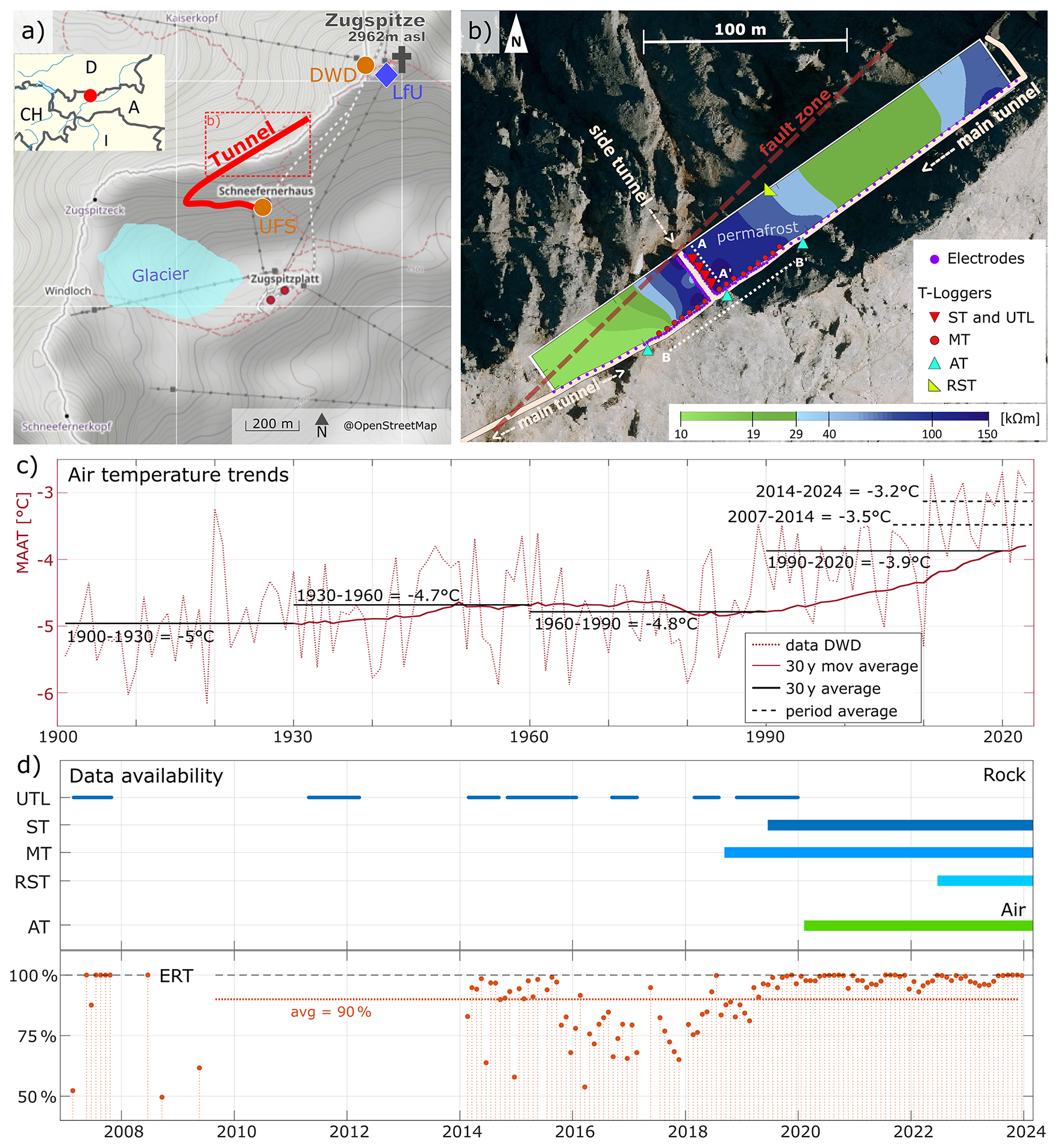
Figure 1 Study site overview. (a) Zugspitze summit, with the DWD meteorological station and the LfU borehole. In red, the main tunnel, going from the research station (UFS) at 2650 m a.s.l. (south) to the exit in the north slope at 2800 m a.s.l. © OpenStreetMap 2023. Open Data Commons Open Database License v1. (b) Zoom of the monitoring site showing the main and the side tunnel, the ERT electrodes, the temperature loggers, and the two temperature transects (A–A' and B–B'). In the background, one exemplary tomogram from Krautblatter et al. (2010) shows the permafrost lens. A red line shows the approximate location of the fault zone. (c) Mean annual air temperature (MAAT) at the DWD station. The thick red line shows the 30-year backward moving mean, while the black lines show the average for the selected period. (d) The upper graph shows data availability for temperature loggers. For abbreviations, consult Table 1. The lower graph shows ERT data availability, with the percentage indicating the number of quadrupoles collected during fieldwork (100 % corresponds to 1310 quadrupoles).

2.3 Monitoring setup

The setup of our study is based on the feasibility study conducted in 2007 and 2008 by Krautblatter et al. (2010) and remained constant to obtain comparable measurements. Monthly monitoring of electrical resistivity (ρ) commenced in 2014 and continues to this day. Measures were undertaken along 6 transects, with electrode distances of 4.6 and 1.5 m, using Wenner and Schlumberger arrays, for a total of 1310 quadrupoles. The monitoring settings are presented in the Supplement (Fig. S1), and a detailed description of the procedures is provided in Krautblatter et al. (2010). Resistivity data were primarily collected using an ABEM Terrameter LS, with alternating use of an ABEM SAS 1000 and SAS 300C before 2018. Contact resistance was improved by spraying the electrodes with saltwater shortly before the measurements, after our tests showed it did not affect the results. Electrodes that still had too high contact resistivity, mostly close to the active layer because of ice on or around the electrodes, were eventually excluded from the measurement. Problematic electrodes with rust or poor coupling have been consistently replaced. The final number of measured quadrupoles reached on average 90 % of the total, but was constantly above this average in the last 5 years (Fig. 1d). Data were collected using a stacking of 2, increased to 4 in case of a measurement error above 1 %. Between 2017 and 2018, data availability and quality were limited due to repeated cable failures; therefore, 14 measurements from this period have been excluded from this analysis.

Table 1 List of all temperature loggers. MT = Main Tunnel, ST = Side Tunnel.

Hourly monitoring of rock temperature (T) follows Krautblatter et al. (2010) with updates and extensions as listed hereafter and in Table 1. Old loggers of Type UTL-1 were replaced with new Geoprecision loggers, offering higher accuracy and reliability. New loggers were installed along the main tunnel at a depth of 40 cm for rock and air temperature (MT and AT). One logger has been installed outside to measure rock surface temperature (RST) at 15 cm depth. The ST, AT, and RST loggers (Geoprecision) were calibrated at 0 °C by the manufacturer using a high-precision water triple-point cell, reaching a temperature stability of ±0.005  °C. This process ensures high accuracy and reproducibility in calibrating the measurement system. The iButton loggers (MT) were calibrated in an ice bath on multiple occasions throughout the study to account for drift effects. The analysis presented here focuses on the period after 2018, where complete data have been recorded. Data availability for temperature loggers is presented in Fig. 1d.

2.4 Data analysis

To analyze temperature dynamics, we linearly interpolated the four temperature measurements along the side tunnel (transect A–A') from 2019 to 2023, treating them as a borehole (Figs. 2 and 3).

Successively, T-ρ field calibration (Figs. 4, 5, and S6) was conducted by combining these temperature values with single apparent resistivity values from the closest quadrupole to each temperature logger (within a 0.3 m radius). Logger ST-5, located at a depth of 5 m below the surface, was excluded from the calibration because resistivity measurements at this location were only available during summer, resulting in an insufficient dataset for robust analysis. To validate the results, we analyzed the probability density function of the apparent resistivity before inversion (Fig. 6).

After field work, each database was imported into MATLAB. Winter measurements from December to June produced, on average, 4 negative resistivity measurements, which were excluded, while summer measurements showed none. Data were filtered using the coefficient of variability (CV, or VAR (%) according to ABEM) of the resistance, i.e., the standard deviation divided by the mean, as computed by the measuring instrument, to remove systematic errors. The threshold for the CV was set to 1 %, resulting in an average exclusion of 6 data points, mostly concentrated in the winter months.

For the ERT inversion, we utilized an updated version of the software CRTomo (Kemna et al., 2000). This inversion algorithm fits a model f(m)_i to the data d_i based on an adequate data error description ϵ_i, instead of just minimizing the data misfit as commonly done. Data fit is achieved when the data misfit ϵ_RMS (root mean square) value is close to one, which indicates that the model reproduces the data within the expected error margins on average, as shown in Eq. (1) (Kemna et al., 2000)

$$\begin{array}{}\text{(1)}& {\mathit{ϵ}}_{\text{RMS}}=\sqrt{{\displaystyle \frac{\mathrm{1}}{N}}\sum _{\mathrm{i}}^N{\left|{\displaystyle \frac{d_{\mathrm{i}}-f(\mathit{m}{)}_{\mathrm{i}}}{{\mathit{ϵ}}_{\mathrm{i}}}}\right|}^{\mathrm{2}}}.\end{array}$$

Following Krautblatter et al. (2010), we performed independent inversions without applying a time-lapse approach. Because time-lapse inversion can significantly influence results (Scandroglio et al., 2021), we aimed to minimize temporal constraints, such as those introduced by prior or initial inversions, that may bias the results. We argue that this approach enhances the robustness of our results, as consistent trends emerge without temporal regularization.

Further on, the error model for the inversion was updated with new measurements. Image quality is highly dependent on the error estimates in the inversion: an overestimation smooths the image, reducing resolution, while an underestimation leads to artifacts (Binley et al., 1995; LaBrecque et al., 1996; Slater et al., 2000; Lesparre et al., 2017; Tso et al., 2017). The random error (e) can be quantified using the difference between normal (R_N) and reciprocal (R_R) resistivity measurements, although this is only a measure of precision and not accuracy (LaBrecque et al., 1996) and does not represent the total experimental error. The error can be modeled as a linear function of the mean resistance R (Eq. 2), depending on an absolute (a) and a relative (b) term

$$\begin{array}{}\text{(2)}& |R_{\mathrm{N}}-R_{\mathrm{R}}|=e=a+bR.\end{array}$$

To solve this, Slater et al. (2000) expresses R as a function of e, removes obvious outliers (e>10 % R), and obtains a and b from the envelope of all remaining measurements. Koestel et al. (2008) instead rejected only values of e>100 % R and then divided the measurements into logarithmically equally sized bins. The standard deviations of the reciprocal errors in each bin were least-square fitted with the linear error model (Eq. 2). Lesparre et al. (2017) adapted the approach of Slater et al. (2000) to fit the discrepancies between readings acquired at different times, proposing data error estimates for time-lapse measurements.

After updating the used error estimates, we computed a new inversion for all measurements, including those from 2007 published in Krautblatter et al. (2010), and analyzed temporal changes by classifying different areas of the tomogram, such as the active layer and permafrost core. Some authors manually define an area of interest (Kneisel et al., 2014), while others choose an automated algorithm (Delforge et al., 2021; Watlet et al., 2023). Here, the inversion results were clustered using the MATLAB k-means algorithm. The function analyzed all tomograms from 2014 to 2023 and computed, for each grid cell, the squared Euclidean distance to the cluster centroids (the cluster means). Cells were then categorized into the nearest centroid. The number of clusters k is defined by the user, and assignment is mutually exclusive. This approach converges to a local minimum, though lower minima may exist. In practice, the global minimum is approximated by running multiple replicates with random starting points. We used five cluster classes, based on the elbow method (Cimpoiasu et al., 2025), which evaluates the sum of squared distances between samples and their nearest cluster center as a function of the number of clusters. The optimal number is identified at the elbow of the resulting curve.

3 Results

3.1 Characterization of thermal regime from temperature measurements

The temperature distribution in the tunnels indicates permafrost presence in transect A–A' (Fig. 2). Due to repeated measurement gaps before 2019, it is not possible to determine longer temperature trends. Over the last five years, the increase in active layer thickness (ALT) from 8.5 to 10 m, combined with the overall rise in annual maximum temperatures, indicates permafrost degradation. The 10 m logger has now reached 0 °C and maintained this level for more than 2 months in summer 2023. It is likely to overcome this threshold in the next few years. No permafrost is recorded in transect B–B' (Fig. S2, Supplement), while seasonally frozen rock is recorded between electrodes E30 and E39. All loggers in the main tunnel recorded their maximum temperature in 2023, with a more pronounced increase in the area to the right of the side tunnel, specifically electrodes E32 to E41. Outside the tunnel, the mean annual rock surface temperature of the steep bedrock facing north is −1.7  °C (RST-Logger, Fig. 3c).

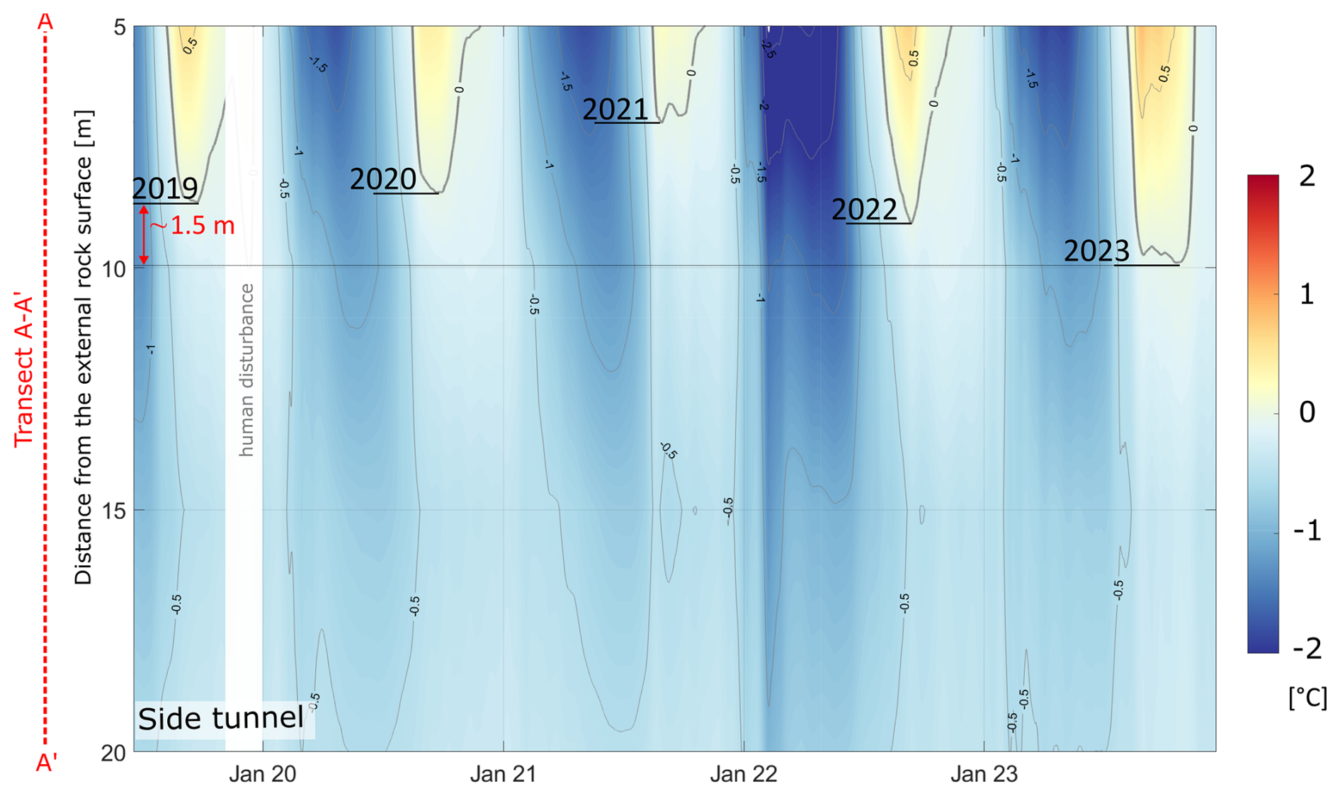
Figure 2 Temperature profile in the side tunnel. The location of the transect is visible in Fig. 1b (profile A–A').

Ice on the ground of the main tunnel decreased between 2019 and 2021, especially in the area of the permafrost lens between electrodes E31 and E38 (Fig. S5). This decrease aligns with the temperature increases recorded by the loggers in the main tunnel. As documented by Scandroglio et al. (2025), large quantities of water from snowmelt are recorded in June and July in the northern part of the main tunnel (electrodes E1 to E20, x=200 to 275 m). In the side tunnel, water accumulation on the ground is also common, but only at the end of summer and between the ST-5 and the north face. This water results from melting surface ice on the tunnel walls and from ice-filled fractures within the tunnel.

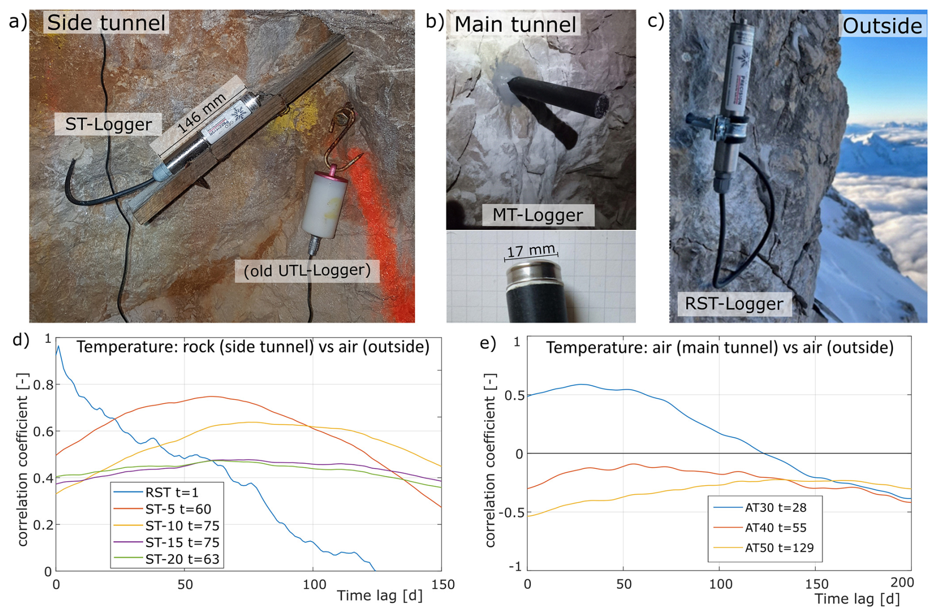
Figure 3 Temperature loggers and their correlation with external air temperature. (a) Photo of the new ST-loggers and the old UTL-loggers. All sensors are located at a depth of 40 cm. The old loggers were replaced in 2019, with a one-year overlapping period. (b) Photos of the MT-loggers, also at a depth of 40 cm. (c) Photo of the RST logger on the north face, close to Electrode E30, at 10 cm depth. (d) Correlation between ST-loggers and external air temperature from the DWD station. (e) Correlation between AT-loggers and external air temperature.

The correlation between rock temperature inside the tunnel and air temperature outside is clear (Fig. 3d), with correlation coefficients between 0.77 for the ST-5 logger at 5 m depth and 0.4 for the ST-20 logger at 20 m depth. As expected, with increasing depth, the time lag grows, reaching up to 75 d at 10–15 m. This represents the time required for the thermal signal to propagate to the permafrost core within the bedrock. The correlation between air temperatures inside and outside the tunnel is strong at electrode 30 (x=143 m), near one of the tunnel exits, but becomes absent for deeper loggers (Fig. 3e), indicating the influence of additional processes at greater depths (e.g., solar radiation or snow cover from the south side slope). A comparison of ST-Loggers with the LfU-borehole (Gallemann et al., 2017), which is installed on the summit, ca. 150–200 m higher than our site, shows that ST-5 and ST-10 are quite similar to the LfU-borehole measurements in summer. At the same time, winter temperatures are much lower in the LfU-borehole (Figs. S3 and S4).

3.2 Field calibration of the T-ρ relation

The newly collected thermal information, together with the ERT measurements, allows us to validate the temperature-resistivity (T-ρ) laboratory calibration by Krautblatter et al. (2010), which was often used to interpret ERT field measurements so far (e.g., Magnin et al., 2015; Etzelmüller et al., 2022; Scandroglio et al., 2021). Figure 4 shows that, despite differences in resistivity ranges, there is a high correlation between temperature and resistivity.

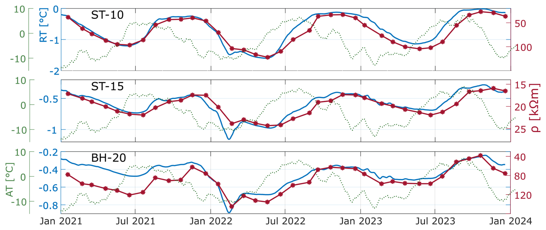
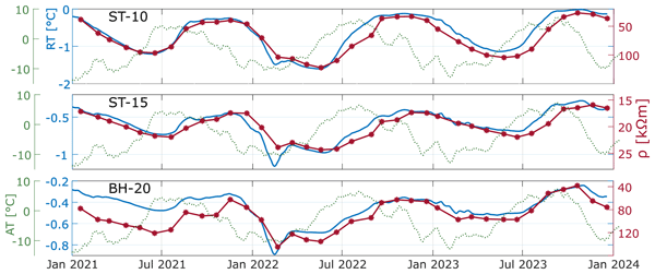
Figure 4 Temperature versus resistivity. Rock temperatures from the ST loggers in blue, and air temperatures from the DWD station in dotted green. In red, single quadrupole apparent resistivity measurements, prior to inversion, with reverse axis direction for simplifying comparison. Other periods are available in Fig. S6 of the Supplement.

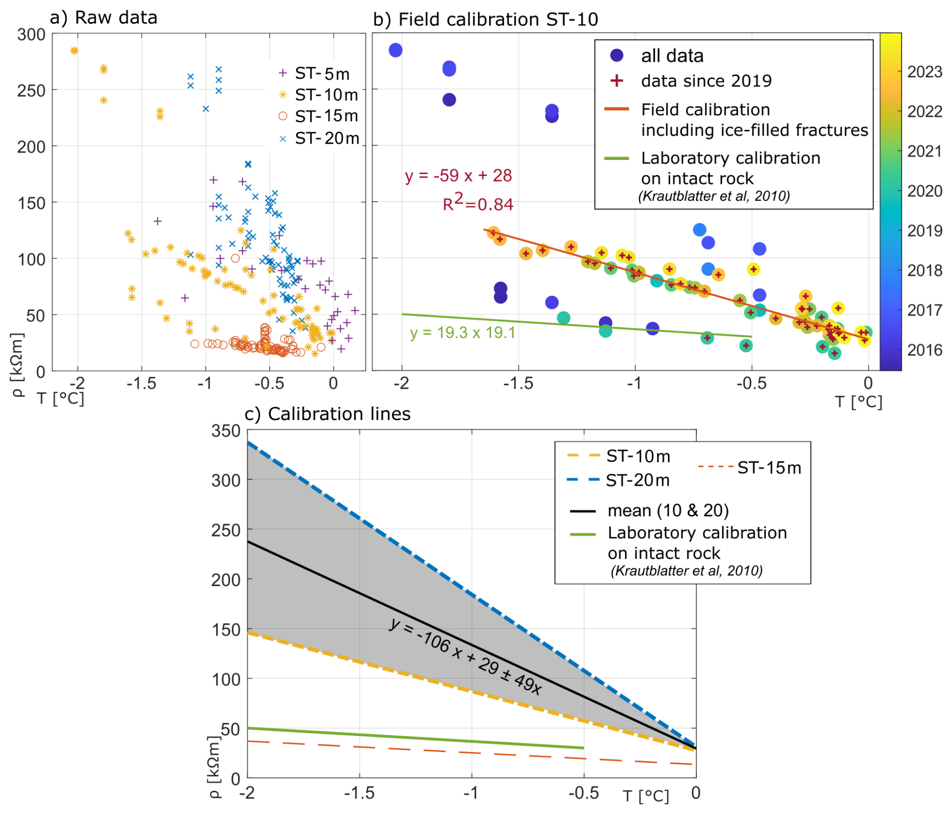
Figure 5 T-ρ field calibration. (a) All values from 2021 to 2024. (b) Calibration for ST-10, using only the values from the new T-loggers, from 2019. In red is the interpolating line, in green is the lab calibration from Krautblatter et al. (2010). (c) Calibration lines for all loggers. In black, the average of logger ST-5, ST-10, and ST-20.

Resistivity varies from 30 to 120 kΩm for ST-10, from 15 to 25 kΩm for ST-15, and from 40 to 130 kΩm for ST-20. These differences lead to a strong spreading of data when plotting all the values together (Fig. 5a). Still, when analyzing each temperature logger separately, the correlation appears clear (Fig. 5b and Fig. S7b–e). This suggests that the relation between resistivity and temperature can not be assumed to be unique for this transect. Logger ST-5 records only a few values below 0 °C: during the cold months, a thick ice cover in the tunnel limits electrode contact, whereas in the warm months, positive temperatures are measured. Therefore, ST-5 will be excluded from our analysis. The other loggers show a good linear fit: the best is at ST-10 (R²=0.84), whereas at ST-20 the fit is poor (R²=0.41). Resistivities decrease over time, possibly due to reduced ice content; therefore, an annual analysis could yield a better fit. Generally, most recorded data are close to the freezing point, which should be taken into consideration. Supercooling effects and similar phenomena from the calibration are not detectable in the field calibration due to the absence of freeze-thaw cycles in the permafrost core.

The freezing point at 29 kΩm agrees with values from the laboratory, but in the field, resistivity increases at much stronger rates than laboratory experiments can reproduce. Field calibration results for ST-10 and ST-20 can be resumed in the “average” Eq. (3).

$$\begin{array}{}\text{(3)}& \mathit{\rho }=(-\mathrm{106}\pm \mathrm{49})T+\mathrm{29}\end{array}$$

ST-15 shows much lower resistivity values than the other locations and behaves similarly to the laboratory calibration. This could depend on the degree of fracturing at this location.

3.3 Field validation of the T-ρ relation

To explain the big discrepancies in the field calibration, we analyze the rock that composes the tunnel. While the majority is made of compact rock (material A in Fig. 6), short parts of the tunnel are highly fractured due to the fault zone (material B in Fig. 6). As suggested by Scandroglio et al. (2021), we compare the probability density function of the apparent resistivity of all the measurements in the permafrost area (side tunnel). The ERT transect on the right (Fig. 6d) presents only one peak, while on the left (Fig. 6c) two peaks are visible. Supposing that each peak relates to a different rock type, this indicates the presence of two materials in the left area, as confirmed by field mapping (Fig. 6a). The probability density curves for material A on the right side of the tunnel clearly show variations with time towards lower values. At the same time, smaller changes are recorded on the left for material A and no changes for material B. A combination of both materials would likely produce results similar to material B, as current follows the easiest path of lower resistivity; however, this should be further investigated.

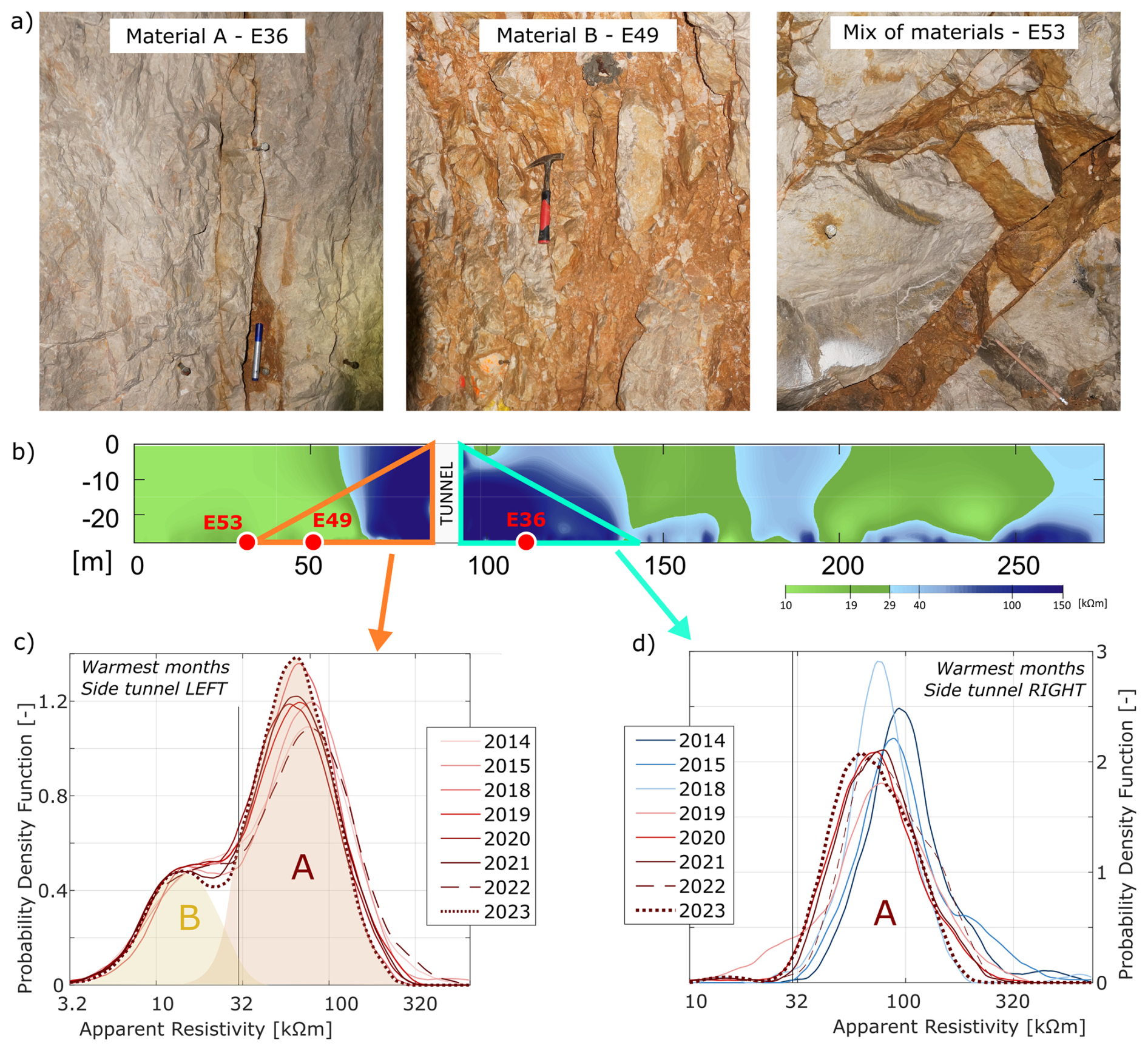
Figure 6 Comparison of ERT raw data for the two resistivity transects in the permafrost area. (a) Photos from the tunnel. Material A, at electrode E36, is pure bedrock. Material B, at electrode E49, is mostly fine-grained material. A mix of materials A and B with fractures of variable width is also possible. (b) Areas of interest of the ERT transects in the side tunnel: violet for the left and yellow for the right transect. (c–d) Probability density functions of apparent resistivity of the whole transect for the warmest months. Data in subplot (c) show two peaks, indicating the presence of two main signatures, while data in subplot (d) shows only a single peak. The year 2023 recorded the lowest apparent resistivities in both cases.

3.4 Error model updating

During previous research at this site, Krautblatter et al. (2010) analyzed 3000 reciprocal measurements according to Koestel et al. (2008) and obtained values of a=48 Ω and b=8 %. We recorded reciprocal measurements for four months in summer and autumn to validate these results and analyzed them using three methods, as described in Slater et al. (2000), Koestel et al. (2008), and Lesparre et al. (2017). All methods suggest that the previous absolute error (a) was strongly conservative. The newly computed value of a approaches zero (a=0.22 Ω), as Fig. 7 shows. The value of b by Krautblatter et al. (2010) appears to be correctly estimated: we obtained b=7.5 % according to Slater et al. (2000), or lower values (b=4 %) according to Koestel et al. (2008) and Lesparre et al. (2017). For the following analysis, we will use the error estimation from Slater et al. (2000), as lower values of b can lead to overfitting in the tomograms.

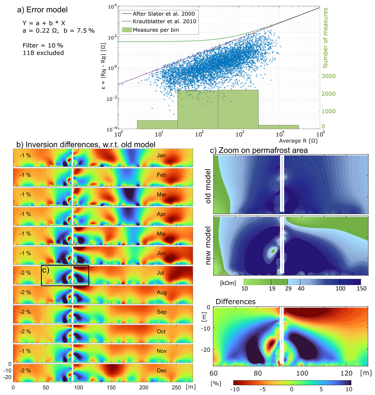
Figure 7 Error model differences. (a) The new error model according to Slater et al. (2000), where each dot represents a normal and a reciprocal measurement. (b) Relative differences between inversions with the old and the new error model for 2022. Resistivity values in log₁₀(ρ). Numbers express the overall change as a percentage. (c) Zoom, subsection of (b) outlined in black. Comparison of the permafrost extension in July: The upper figure is obtained using the old error model; the middle figure, using the new model; and the lower figure shows the differences.

In Fig. 7b, we present the inversion differences between the error model chosen for this study and the model previously used in Krautblatter et al. (2010), applied to the inversion of the ERT monitoring data from 2022. Using the updated error model, resistivities in the permafrost core (x=65 to 115 m) are higher in both winter and summer. The maximum differences occur from May to July, especially on the right side of the side tunnel (an increase of >10 %), while the smallest differences occur between January and April. An exception is represented by the area between y=0 and −10 m right of the side tunnel (Fig. 7c), which is very close to the rock surface. Here, resistivities are generally lower, with peaks during the warm months: this better represents the active-layer dynamics measured with temperature loggers. Considerable differences are also evident in the area corresponding to the fault zone crossing the permafrost body. The inversion with the updated error model reports lower resistivities along the fault axis; however, these values do not extend to the main tunnel, as field observations would suggest. The area between x=150 and 200 m shows higher resistivity, but only in the winter months. The tunnel in this area is covered by concrete (indicating a more fractured bedrock), and it is seasonally covered by ice on the ground and walls. The tunnel surface ($y<-\mathrm{25}$ m) shows smaller differences: frozen patches are found at different x-positions, but the most evident is at x=135 m, which corresponds to one tunnel exit where snow normally accumulates in winter. Lower resistivities are produced by the inversion at x>225 m from January to July, with new values reaching −10 %.

3.5 Characterization of thermal regime from resistivity

Long-term signal

Figure 8 shows all ERT inversion results from 2007 to 2023 using the updated error model. This allows the detection of features, listed hereafter, that are confirmed by field observation (Fig. S10).

• a.

  The active layer is visible from 2014 on, at the right side of the tunnel next to the permafrost core (x=100 and 150 m). This feature follows the structure of the external slope and reaches minimum values from July to September.

• b.

  From December to April, a temporary frozen part appears at the center of the image (x=150 to 200 m). This is an area of the tunnel with reduced rock thickness and a steep bedrock slope outside.

• c.

  The constantly unfrozen part between 200 and 250 m fits with a less steep debris-covered area outside the tunnel, which is snow-covered in winter.

• d.

  Some frozen patches can be found along the tunnel ($y=-\mathrm{25}$ m, lower border of each image), while they are present all year long in 2014 and 2016, decrease, up to disappearing, from 2018 onward.

• e.

  The fault zone crossing the permafrost is evident in all tomograms. This area exhibits lower resistivity than the surrounding area, with no clear thermal explanation.

• f.

  The constantly lower values at the beginning of the tunnel represent the area with the biggest distance to the north slope.

In addition to these features, measurement errors are also evident, thanks to the new error model, for example, in November 2020. For all inversions based on the new error model, RMS values range from 0.97 to 1, and the number of iterations ranges from 3 to 12, with an average of 6. Details are shown in Figure S9b. As expected, the smaller b-value of the updated (or new) error model leads to smaller data misfits and, consequently, to less smooth, slightly more detailed inversion results.

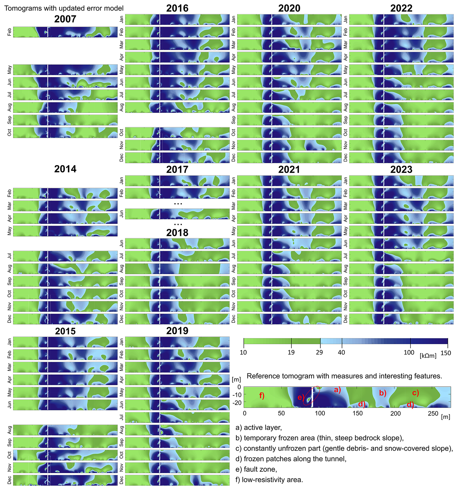
Figure 8 ERT inversion results. Tomograms from 2007 to 2023. On the left, the month of each tomogram. The color bar shown is valid for all tomograms. Bottom right: reference tomogram.

Long-term trends clearly present a reduction of the frozen areas, as confirmed by Fig. 9. While frozen areas increased from 31 % to 40 % of the total area between 2007 and 2014, they drastically decreased from 2014 to 2020 to 25 %. This corresponds to a 40 % reduction compared to 2014. The last four years present little variation in the minimum frozen area. These trends are also visible in the winter months, but are less pronounced.

Figure 9 Long-term development of the frozen areas, from 2007 to 2023.

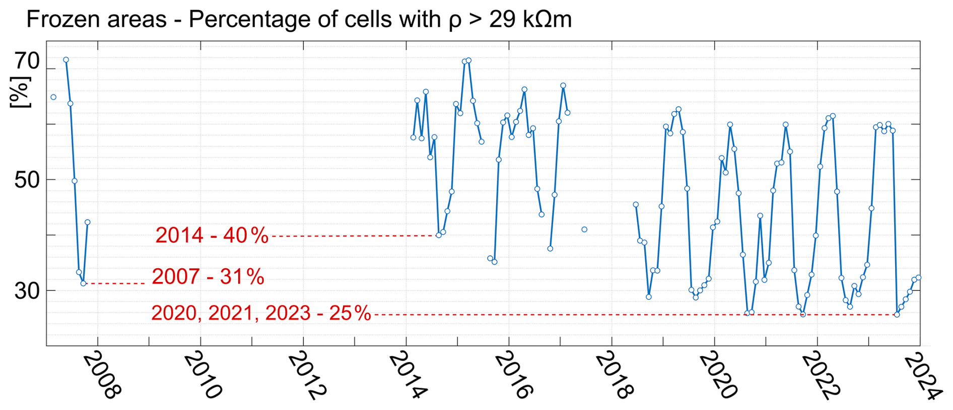
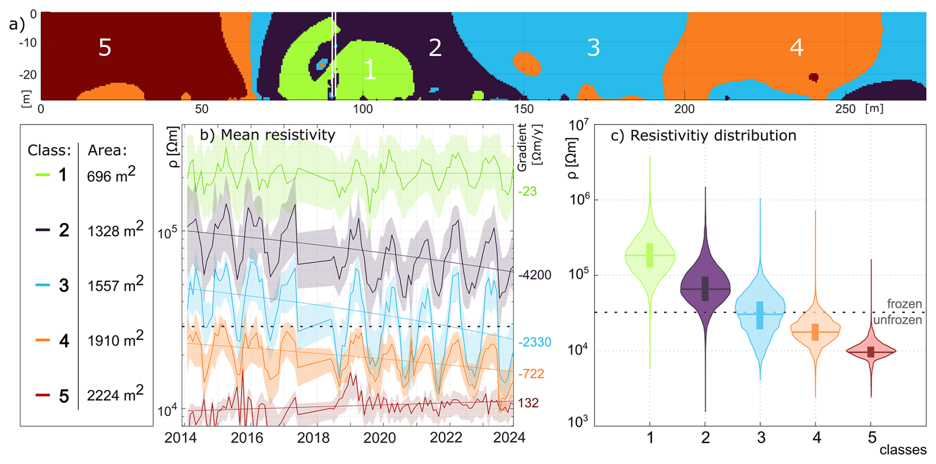
Figure 10 k-means clustering. (a) Classified tomogram. (b) Mean resistivities for each class on a logarithmic scale. On the left, the areas covered by each class are listed, and on the right, the corresponding gradients are shown. (c) Violin plot of all resistivity values included in one class.

Image clustering of the tomograms with k-means

The best fit between the measurements and the previously analyzed features is obtained with k=5, as confirmed by the elbow method. The results are presented in Fig. 10. Class 1 shows the highest ρ values, which correspond to constantly frozen rock. This class has been remarkably consistent over the last 10 years and represents the core of the permafrost. Classes 2 and 3 include cells that are, respectively, mostly frozen and partially frozen, representing rapidly degrading permafrost and the active layer. Both classes are experiencing the strongest decrease in ρ (−4200 and −2330 Ω my⁻¹, Fig. 10b). Class 4 comprehends mostly unfrozen cells with a slightly decreasing 10-year trend and represents feature (c) of Fig. 8. Class 5 encompasses the unfrozen area at the beginning of the tunnel, which has exhibited slightly increasing values over the past decade but has undergone constant development recently. The distribution of values in Fig. 10c shows all values and not only the mean. In particular, values in class 2 are mostly frozen, while those in class 3 are half frozen and half unfrozen.

Quantification of changes in permafrost extent

Knowing the grid size, we can estimate the size of the permanently frozen area. It covers circa 2000 m², of which 700 m² is in class 1 (35 %) and 1300 m² is in class 2 (65 %). The external morphology suggests a vertical extension of the lens of 20–30 m, which would result in 40 000–60 000 m³ of frozen rock. The remaining temporarily frozen and unfrozen areas (classes 3, 4, and 5) cover 5700 m², about 75 % of the tomogram. Given the strong decreasing rates in the outer layer (class 2), up to 39 000 m³ of permafrost are very likely to suffer irreversible thermal degradation, potentially leading to its disappearance. By linear extrapolation of the gradient computed in Fig. 10b, we expect this process to happen within the following decade. This assumption significantly simplifies complex physical processes that are not necessarily linear and should therefore be considered with some degree of uncertainty. Still, given the actual development of climate change, the trend is unquestionable.

Quantification of seasonal variations

To detect seasonal trends, we used the mean ρ value across the entire ERT tomogram. The maximum values are recorded in April or May, the minimum around September (±1 month), as shown in Fig. 11a. In the summer months, there is a clear shift in time towards lower values of ρ, while this is less evident in the winters, which present a higher variability. Resistivities in 2023 (dark red) indicate a prolonged winter with low values, a drastic drop in resistivities from June to July, and a long summer season with extremely low values from July to October. Comparing ten years of records reveals three distinct phases. The first is a gradual increase in resistivity from October to March/April. There is a sudden decrease between May and July, and finally, a stable phase with little variation in resistivity from August to October.

Seasonal averages in Fig. 11b show that the resistivity decrease in the last ten years is more pronounced in the spring and summer months, reaching more than 0.9 kΩm yr⁻¹. Winter values are decreasing less than one-third of the rate. While winter and spring values vary widely from year to year, summer averages follow a clear linear trend.

Figure 11c shows that the tomogram's mean ρ is strongly correlated with the mean monthly air temperature with an hysteresis pattern. Resistivity responds to temperature changes with about a two-month delay, producing an elliptical path. The change in time (described by colors) shows the evolution over the last 10 years towards warmer air temperatures (+2 °C in summer), which led to lower resistivity (−8 kΩm). 2023 recorded the lowest value both for ρ and MAAT: 4.8 °C and 19 kΩm.

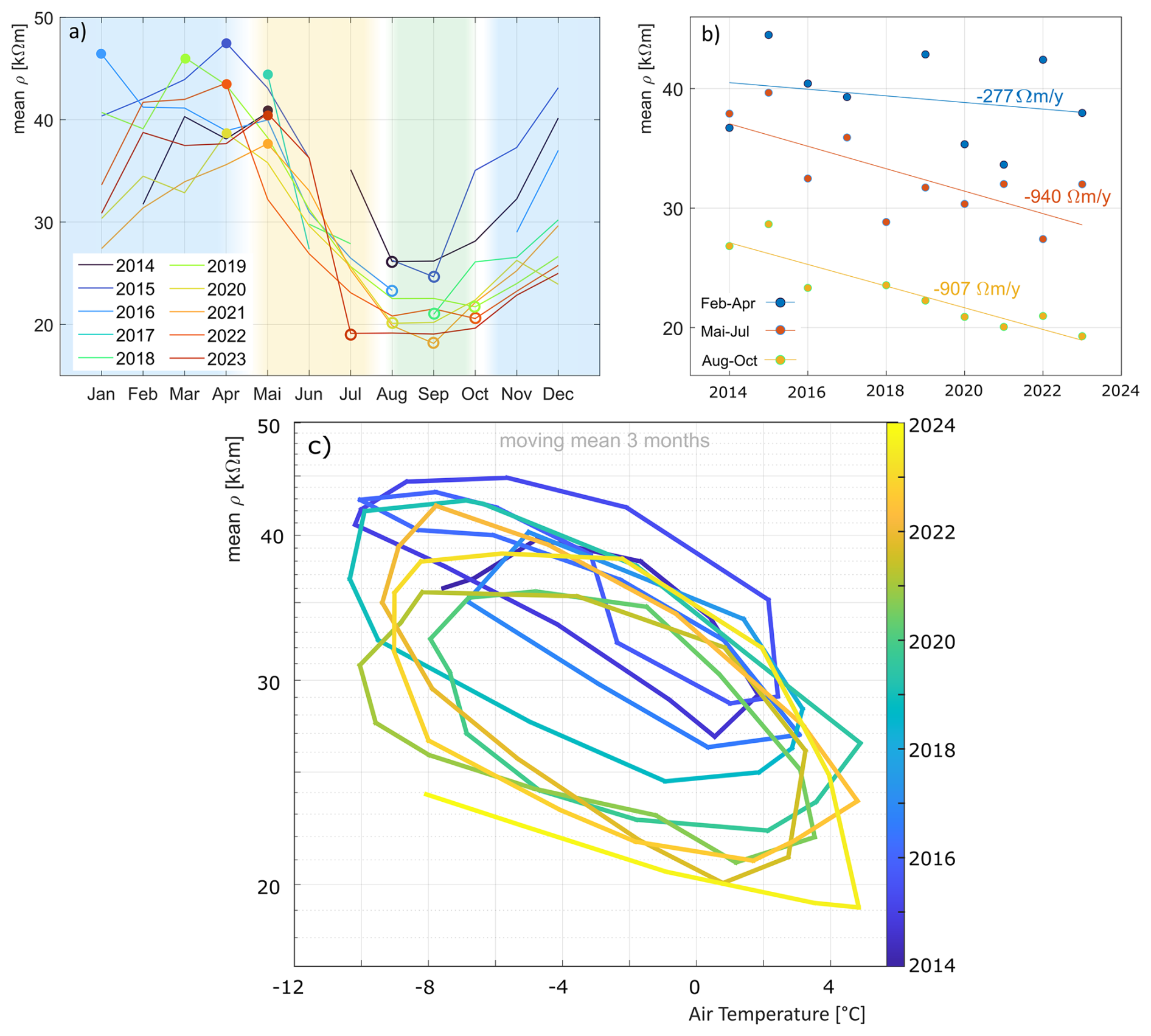
Figure 11 Seasonal changes of mean resistivity. Average value of the entire ERT tomogram, from 2014 to 2023. (a) Seasonal variation for all years. (b) Average values of 3 months, with trendline and gradient: February, March, and April in blue, May, June, and July in red, and August, September, and October in yellow. (c) Comparison of the tomogram mean resistivity with the mean monthly air temperature, measured at the DWD station on the summit, both values as a 3-month moving mean.

4 Discussion

We present 15 years of monthly ERT profiles and investigate permafrost dynamics in steep bedrock applying a newly developed temperature-resistivity (T-ρ) field calibration, and an updated error model, compared to the first studies by Krautblatter et al. (2010). Newly available data, improvements in methods, and updated analyses have significantly enhanced the quantification of both short-term permafrost dynamics and long-term degradation.

4.1 Linking temperature and electrical resistivity: comparison between laboratory and field observations

Precise knowledge of the T-ρ correlation is crucial for a correct interpretation of the thermal state of the permafrost core derived from resistivities. Many laboratory calibrations are nowadays available for different sites and materials (examples in Herring et al., 2023; Limbrock et al., 2025), but most studies do not validate them quantitatively in the field (e.g. Magnin et al., 2015; Duvillard et al., 2021). Information at permafrost core depths is often missing, as few studies have compared field and laboratory measurements. Mollaret et al. (2019) previously conducted field calibration but did not compare it with laboratory values. Offer et al. (2025, 2026) reported lower resistivity values in field measurements compared with laboratory calibrations, attributing this discrepancy to water pressure effects. To date, no field calibration procedures have been proposed.

Krautblatter (2009) demonstrates that resistivity behaves differently above and below the freezing point, a finding that we also observed at the ST-5m logger (see Fig. S7b). He could also show that the ρ-T gradient below the freezing point (29.8±10.6 % °C⁻¹) is, on average, ten times higher than that above the freezing point (2.9±0.3 % °C⁻¹). Our new field calibration yields similar values at the freezing point, but higher resistivity gradients at low temperatures. Similar results are obtained when comparing field calibration by Mollaret et al. (2019) with laboratory measurements by Hauck (2001), or for laboratory measurements consistent for different types of rocks Limbrock et al. (2025).

Assuming that laboratory measurements are typically performed on intact rock samples, it can be inferred that such results provide a reasonable approximation of a saturated rock matrix. Laboratory calibrations are typically performed on fully saturated samples, whereas field conditions often involve partial saturation, which can result in higher resistivity. In this case, the conditions we observe at the Zugspitze are always nearly fully saturated (>90 %), except for the outer 8–10 cm of the rock surface (Sass, 2005). In the specific setup where we measure from inside the gallery, meters to decameters from the rock wall, surface variations do not play an important role (compared to measurements with electrodes on the surface). The higher resistivity values observed in the field are likely attributable to the presence of ice within frozen discontinuities. However, the extraction of rock samples inevitably removes them from their in situ stress conditions, which may induce minor fracturing or the opening of pre-existing fractures, thereby potentially reducing the measured resistivity of the specimen.

Additionally, Krautblatter et al. (2010) recorded supercooling effects just after the equilibrium freezing point (−0.5 °C) during initial freezing in laboratory tests. Although these effects are not directly apparent in our dataset, an increase in the standard deviation of resistivity measurements is observed near the freezing point in the ST-5m logger data (see Fig. S7b), which may be linked to similar processes. It is important to note that such effects were only observed in the laboratory during the initial freezing phase and for very short periods, conditions that cannot be replicated with our setup.

Both field and laboratory calibrations at our site agree on the freezing point around 29 kΩm; however, the interpretation of laboratory measurements above this point should be taken with caution. In fact, it is impossible to accurately reproduce the steadily variable alternation of bedrock, fractures, ice/water, and voids found in nature in a sample; however, this composition strongly influences ERT results. This is evident in the high variability of the calibration results presented here, despite our temperature loggers being just 5 m apart. For this reason, caution should be exercised when extrapolating the T-ρ relation to other locations, even within the same site. We suggest that field calibrations are totally valid only for the measured spot. Further limitations are a reduced temperature range in nature and the lack of freeze-thaw cycles when measuring permafrost. Recent studies confirm the presence of hysteresis effects in field measurements and demonstrate their importance in the energy balance of permafrost (Limbrock et al., 2025; Luo et al., 2024; Tomaškovičová and Ingeman-Nielsen, 2024).

Our measurements recorded resistivities greater than 200 kΩm, values that exceed the laboratory calibration range. Krautblatter et al. (2010) has explained these values in terms of ice presence, but not numerically proven. Our results indicate that laboratory calibration should be validated in the field and, if necessary, refined based on field data.

4.2 Influence of the error model on long-term ERT measurements

The chosen procedure, the filtering criteria for outliers, and the bin placement can affect the quantification of the error to varying degrees (Koestel et al., 2008; Tso et al., 2017). Different arrays generate distinct error types, corresponding to different error models. Further complexity arises when multiple measurements are combined into a single dataset, as in this case. In addition, the reciprocal error may vary over time during long-term monitoring due to changing external conditions, such as seasonal fluctuations in water state or long-term variations in underground water content. Given these factors, the best inversion would theoretically require one error model per array and per epoch, which would be time-consuming during data acquisition. As a consequence, the use of reciprocal errors is very rare in field applications (Herring et al., 2023). When reciprocal measurements are conducted, most studies use a uniform error level for all configurations and time steps to reduce the degrees of freedom (Lesparre et al., 2017; Tso et al., 2017), thereby ensuring consistency among results at different times (Krautblatter et al., 2010; Maierhofer et al., 2024), while other authors use a time-varying error model (Koestel et al., 2008). With the new computation of the error model suggested here, i.e., the drastic reduction of the absolute term a, we possibly introduce some artifacts in the inversion results. Still, the significant advantage is a substantial increase in resolution, enabling us to investigate permafrost degradation in much greater detail (see features in Fig. 8).

As shown in Figure S9a, the updated error model has little impact on the RMS error, which remains within the same range (0.99–1), as expected, since this is the value minimized by the inversion algorithm. However, the number of iterations increases from 3–4 to 6, which was also foreseeable, since smaller errors require a more precise fit of the model to the data to achieve the same RMS values and therefore more iterations. Inspection of the RMS formulation (Eq. 1) shows that, if ϵ_RMS remains approximately constant, smaller values of the error ϵ_i result in a reduced data misfit (i.e., d_i−f(m)_i). In our case, with the newly computed values of a (Fig. 7), we observe smaller errors for R<10⁴ Ω, leading to stronger data weighting. This, in turn, allows for closer model adjustment, potentially improving the fit, though it also increases the risk of overfitting and introduces model artifacts, while reducing smoothing and enabling the resolution of finer-scale features.

4.3 Permafrost degradation according to ERT

New temperature calibrations and error models enable us to accurately interpret the inverted resistivities, particularly in the permafrost core. Results confirm the presence of permafrost near the melting point, and its degradation is readily quantifiable. Still, complex inter-annual behavior due to latent heat effects during thawing, seasonal water infiltration, and variable snow cover makes the processes highly non-linear (Hauck and Hilbich, 2024) and therefore difficult to interpret. The degree of fracturing also seems to contribute to this non-linearity. A survey of fractured zones was already presented in Krautblatter et al. (2010), but the effects of the fault zone were neglected. Here, thanks to the new field calibration, differences are distinctly highlighted. Clustering, as suggested by Delforge et al. (2021) and Watlet et al. (2023), also provided powerful insights in this direction. Thanks to simple algorithms, large amounts of data are used to detect similar patterns, yielding an objective, data-driven analysis. This allows for a more robust interpretation of results than the “user-defined areas of interest”, which are mostly rectangular, as previously used in the literature (Kneisel et al., 2014).

Despite this complexity at high temporal and spatial resolution, when looking at slope scale over one decade, it is evident that ERT values strongly correlate with rock and air temperatures, as shown in Fig. 12b. Mean resistivity of the tomograms decreases from 37 kΩm in 2018 to 28 kΩm in 2023 (−25 %). The decrease is stronger from 2018 to 2021, whereas in the last 3 years it is less pronounced. Meanwhile, air temperatures have steadily increased since 2012, rising from −4.2 to −3.2 °C.

This supports the theory that external thermal forcing and conductivity are the primary processes promoting permafrost degradation here. Contradicting trends, such as the increase in frozen areas between 2007 and 2014, as shown in Fig. 9, can also be explained by thermal forcing (e.g., rising air temperatures). In fact, the hydrological year 2006/2007 recorded extreme temperatures, 1 °C warmer than the 30-year average. On the contrary, from 2007 to 2014, temperatures were mostly below the 30-year average (Fig. 12b, inlet). Therefore, 2007 can be considered an anomaly, and the measurements from that year are not representative of the 2000–2010 decade.

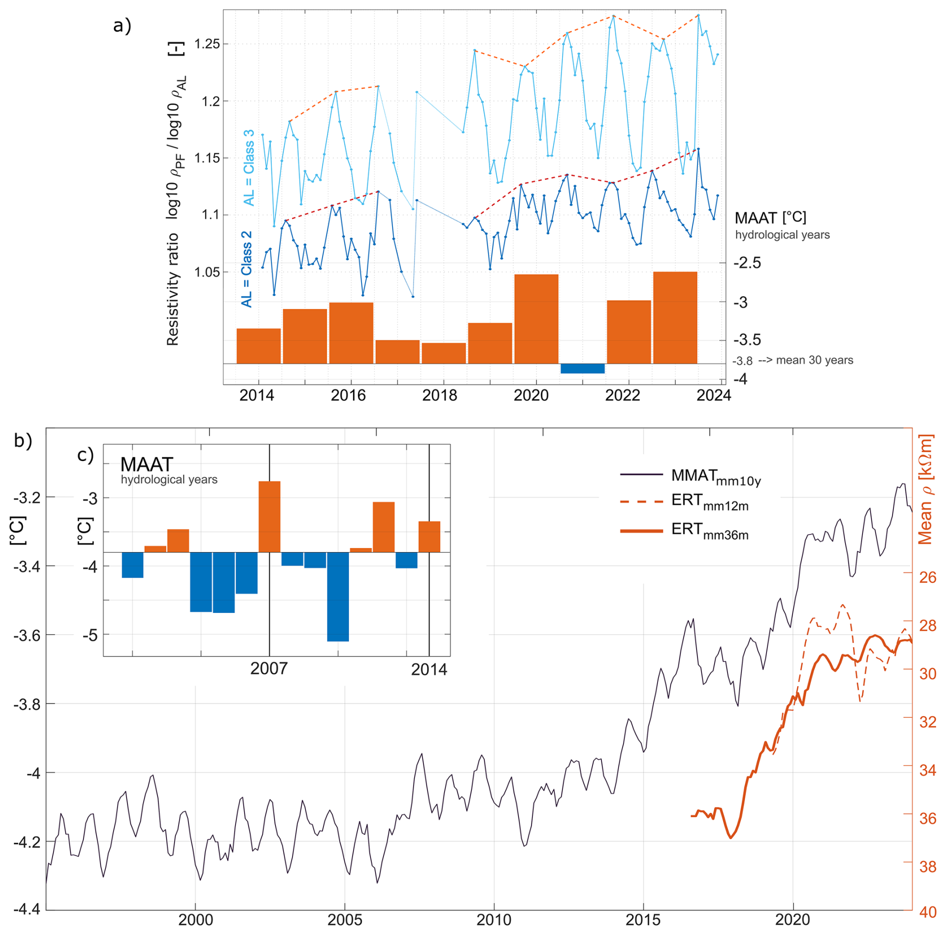
Figure 12 External thermal forcing drives resistivity changes in the active layer. (a) Resistivity ratio: class 1/class 2 in dark blue, class 1/class 3 in light blue. The red lines unite the minimum values for each year. Lower bars: mean annual air temperatures (MAAT) of hydrological years from 2014 to 2024. (b) The increase in overall mean resistivity (in red) is well explained by the increase in air temperature (in black). (c) Inlet: MAAT of hydrological years from 2001 to 2014. The following abbreviations are used: MMAT (monthly mean air temperature), mm10y – moving mean 10 years, mm12m – moving mean 12 months, mm36m – moving mean 36 months.

Analyzing the resistivity ratio between active layer and permafrost ${\mathit{\rho }}_{\mathrm{PL}}/{\mathit{\rho }}_{\mathrm{AL}}$ as suggested by Hauck and Hilbich (2024), we compare clustering class 1 with class 2 and class 1 with class 3 and focus on the maximum values of each year (Fig. 12a). Although they varied, both ratios increased over the last 10 years. The ratio class 1/class 2 closely follows the trends of mean annual air temperature (MAAT): it decreased in 2018 and in 2021 after mild years, while it increased in all other years. In 9 out of the last 10 years, MAAT was above the long-term average of −3.8 °C, with records reaching −2.6 °C in 2019/2020 and 2022/2023. Excluding the possibility that the permafrost core has increased its resistivity (ρ_PL), this trend can be explained only by a decrease in resistivity in the active layer (ρ_AL), to a stronger degree than the decrease in the core, as confirmed by Fig. 10b. Compared with Fig. 9, it is remarkable that, although the number of frozen cells has not decreased since 2021, the ratio ${\mathit{\rho }}_{\mathrm{PL}}/{\mathit{\rho }}_{\mathrm{AL}}$ increased in 2022 and 2023. This confirms that non-linear degradation processes are occurring in the active layer and that sudden degradation may occur in the next few years. On the contrary, it seems that class 1/class 3 have stabilized over the last four years, possibly indicating that degradation has already reached a stable level in these areas.

The resistivity ratio between the active layer and the permafrost in our data falls within the same range as reported by Hauck and Hilbich (2024). However, while they observed a long-term decrease in this ratio, our results show a contradictory overall increase. This suggests that, at our site, the degradation of the active layer has not yet significantly impacted the permafrost core. Notably, our unconventional measurement setup–conducting measurements from the inside out rather than from the surface may influence this interpretation. In typical surface-based ERT surveys, accuracy decreases with depth due to the limited number of data points, resulting in higher confidence near the surface and lower confidence at greater depths. The configuration used here yields improved accuracy along the main tunnel (deep bedrock) and along the side tunnel (permafrost core), but provides lower resolution for the rest of the outside bedrock slope.

4.4 Lessons learned from over a decade of monitoring

After more than a decade of monitoring, we share key lessons learned from challenges like equipment malfunctions and data inconsistencies to improve future monitoring efforts and contribute to the scientific community. Long-term monitoring requires strict consistency in measurement parameters and procedures to ensure data comparability over time. However, when changes in software, hardware, or operational protocols are necessary or beneficial, it is advisable to implement an overlap period during which both the old and new setups are operated simultaneously. This overlap should be sufficiently long to capture variability across different environmental conditions, including both warm and cold periods.

Instruments deployed in humid environments are particularly susceptible to corrosion, which can compromise data quality and equipment longevity. Regular inspection and maintenance are therefore essential and require the continuous replacement of faulty or degraded electrodes. All components of the monitoring system, including cables, measurement units, and data loggers, should be routinely tested to promptly detect and address failures. Immediate, on-site verification of collected data – especially at remote locations – is strongly recommended to identify potential issues early. Quality control procedures – such as threshold checks, outlier detection, and trend analysis – in the data workflow can help identify inconsistencies early. Establishing clear criteria for data validation and flagging enhances the overall reliability of the dataset. In this context, optimizing and automating data analysis procedures can significantly enhance efficiency and reliability.

Comprehensive documentation, regular calibration (with redundancy where possible), and robust data management – including automated logging, standardized formats, and secure backups – are essential to ensure the accuracy, reproducibility, and long-term usability of monitoring data. We also encourage the publication of data in open-access repositories and active participation in collaborative initiatives such as the IPA Action Group IDGSP.

4.5 Future development of permafrost degradation and slope stability

At this site, permafrost degradation is mainly driven by thermal forcing, as shown in Fig. 12b. Future heat waves are projected to increase in magnitude and frequency (Lin et al., 2022). As a result, this trend is expected to persist in the coming decades, particularly for the active layer (cluster classes 2 and 3), although the permafrost core (class 1) will ultimately be affected as well. The fault crossing the tomogram, clearly visible thanks to the newly developed error model, may further accelerate degradation due to its high permeability. In fact, when unfrozen, it could allow large volumes of water to infiltrate, as demonstrated in Scandroglio et al. (2025), thereby introducing advective heat transport processes that compound the thermal degradation. Consequently, atmospheric forcing is expected to play a significant role in the dynamics of permafrost degradation; however, its influence remains difficult to quantify. Increasing the measurement frequency from April to July could provide valuable insights into the delayed thermal response of deep rock layers.

On steep slopes, the increase in rock temperatures is also linked to irreversible ice losses (Hauck and Hilbich, 2024). Although this is not expected to influence the hydrological cycle in alpine environments strongly, it has strong stability consequences for slope stability (Krautblatter et al., 2013). This might also be true for the analyzed area, where the fractured zones might be a source of new instabilities, given the almost vertical dip of this fracture area.

The current setup was not fully automated and, consequently, it does not enable real-time monitoring. The potential of automated ERT has been assessed in Keuschnig et al. (2017). The calibration and error estimates in this paper contribute to a more robust implementation of ERT in monitoring and early warning systems for critical infrastructure, e.g., mountain huts and cable car stations, where less-calibrated approaches are currently being tested. Fixed and automated ERT monitoring systems have been implemented on steep permafrost slopes (e.g., studies by Abdulsamad et al., 2026; Offer et al., 2026). In principle, such systems allow continuous resistivity measurements and could provide near-real-time insights into permafrost conditions. However, to our knowledge, these approaches have not yet reached a level of maturity that enables reliable operational use for early warning purposes. Achieving this would require developing robust automated workflows for both data acquisition and processing and establishing clearly defined early-warning criteria. Potential criteria could include thresholds for active-layer thickness or for resistivity values approaching the thawing point. It is important to remember that ERT-derived information alone is insufficient for early warning applications. It must be complemented by detailed geological characterization, including surface fracture mapping and, ideally, subsurface information obtained from boreholes (Offer et al., 2026) or tunnels to identify critical discontinuities and preferential ways for water flow. Furthermore, reliable quantitative interpretation of resistivity data requires field calibration over at least one complete freeze-thaw cycle and across multiple depths, as demonstrated in this study.

5 Conclusions

This study compiles 109 ERT measurements collected over 17 years at monthly frequency from the Kammstollen Tunnel, 2800 m a.s.l. on Mount Zugspitze (Germany/Austria). Developing a field calibration of the temperature-resistivity relation, improving the inversion error model, and automatically clustering the results advance the understanding and quantification of permafrost degradation in steep rock slopes.

• ERT field-based calibration with rock temperatures over five years validates laboratory-based calibrations, which have become a standard approach in the literature. While both methods show good agreement at the freezing point, field data reveal significantly higher resistivity values at subzero temperatures and highly variable results. This highlights the need for caution when interpreting tomograms based solely on laboratory calibration.

• A correct estimation of measurement errors is essential for a correct inversion and interpretation of ERT data. Regular validation and update of the error model over time can significantly enhance the detection of thermal processes in long-term monitoring.

• Mean resistivity of the tomogram shows a decrease of 25 % in the last 10 years, with more enhanced degradation in the summer months, where the overall decrease rates reach −0.9 kΩm yr⁻¹.

• Frozen cells decreased by almost 40 % in the same period, and the active layer suffered the strongest losses, with rates between −4.2 and −2.3 kΩm yr⁻¹.

• The strong meteorological variability between years requires at least monthly monitoring in the summer and autumn months to precisely assess long-term degradation. Monitoring the spring and winter months is crucial for a comprehensive understanding of the processes and an accurate evaluation of the yearly trends.

• The extent of the permafrost lens in 2023 can be estimated in 2000 m² (Class 1 and 2) – up to 60 000 m³. The actual degradation rates indicate that approximately 1300 m² (class 2) – up to 39 000 m³ – will become unfrozen within the next decade. Still, degradation is not always linear, and this estimation does not account for thermal advection caused by infiltrating water (Scandroglio et al., 2025), which could entirely enhance this phenomenon.

• The proposed resistivity-temperature monitoring allows a quantitative investigation of changes in the thermal regime of permafrost. Compared to previous studies, the results confirm the presence of the permafrost core, but indicate differences in its spatial extent, providing a more accurate representation of its dynamics.

These innovations enhance the ability to detect and predict permafrost degradation and the consequent bedrock instabilities with greater spatial and temporal precision. These findings help decision-makers assess the increasing risks posed by rising temperatures to both society and infrastructure.