Nondimensional parameter regimes of Arctic ice keel-ocean flow interactions and internal wave drag

Sea ice keels influence momentum transfer between the drifting ice cover and the upper ocean, yet their effects remain difficult to represent in large-scale models. When keels move relative to the stratified ocean, they can generate internal waves that contribute an additional drag and modify upper-ocean energetics. We examine the parameter space governing ice keel–ocean interactions by reformulating an existing internal wave drag framework in terms of four nondimensional parameters that quantify lee wave radiation, flow nonlinearity, stratification strength, and the depth of the keel relative to the mixed layer. Using output from a pan-Arctic coupled sea ice–ocean model, we apply Gaussian Mixture Modeling to these parameters to identify statistically coherent regimes across the Arctic for annual, summer, and winter conditions. The resulting regimes exhibit clear spatial organization and pronounced seasonal variability. To interpret their dynamical significance, we perform idealized numerical simulations for representative parameter combinations and analyze kinetic energy dissipation and propagation of internal waves below the pycnocline. The simulations indicate that deep and steep keels beneath perennial sea ice, in particular in the summer when the mixed layer is shallow, enhance dissipation around and below the pycnocline. Comparison with existing parameterizations further suggests that regimes characterized by strong nonlinearity or shallow mixed layers may be not well-represented. These results provide a framework for constraining physically relevant parameter regimes for ice keel drag and inform future model development and observational studies of ice–ocean coupling.

1 Introduction

Sea ice keels, formed by rafting and overturning of pressure ridges, extend several meters below the surface, representing a crucial yet under-explored aspect of Arctic ice dynamics. Their morphology reflects past mechanical forcing – such as ice convergence and interactions with the ocean and the atmosphere (Parmerter and Coon, 1972; Kharitonov and Borodkin, 2020) – and exerts lasting influences on ocean processes beneath the ice.

When ice is in free drift, i.e. internal stresses are negligible, the total ice-ocean stress can be thought to comprise of three main components: (1) the skin drag, (2) form drag, and (3) internal wave (IW) drag (McPhee and Kantha, 1989; Brenner et al., 2021). Skin drag is due to the small-scale roughnesses of the sea ice, and form drag is due to ice keels presenting as discrete obstacles to the flow. Both of these processes play an important role within the turbulent ice-ocean boundary layer (Shirasawa and Ingram, 1991). The transfer of momentum from the moving sea ice to the ocean through these drag forces is typically represented using a quadratic drag law with parameterized drag coefficients. Skin and form drags have been subject to parameterizations in terms of ice keel geometry in many previous modeling (e.g., Lu et al., 2011; Tsamados et al., 2014; Wang et al., 2025) and observational studies (e.g., Cole et al., 2017; Brenner et al., 2021; Kawaguchi et al., 2024; Reifenberg et al., 2025). While there are still many open questions in our understanding of these stress terms, e.g., seasonal and spatial variability and mismatch between geometry-based drag parameterizations and direct measurements (Brenner et al., 2021), in this study, we specifically focus on the IW drag.

When drifting over a stratified ocean, keels act as moving topographic features that perturb density interfaces, generating IWs that radiate away from the ice–ocean boundary transferring additional momentum from the moving ice keels into the ocean (Flocco et al., 2024). This downward momentum flux by the radiating IWs modifies the force balance on the ice, creating drag or resistance (McPhee and Kantha, 1989). Theory of IW generation by moving an object, such as a ship or ice, along the surface of a stratified ocean dates back to the “dead water” effect (Ekman, 1904; Morison, 1986). Roughness on the underside of the sea ice, i.e., ice keels, further promotes IW generation. Reframing the problem to be in the frame of reference of the moving ice keel (Rigby, 1974; McPhee and Kantha, 1989; Pite et al., 1995), this mechanism can be modeled akin to the flow-topography interaction.

In the classical flow-topography interaction problem, lee waves, which is the category of IWs of interest here, are generated when a steady flow has to go over a topographic obstacle, such as a seamount, in the presence of constant stratification (Bretherton, 1969; Bell, 1975). Topography is typically represented as horizontally periodic sinusoidal bumps. The generated lee waves radiate upward away from the topography and the problem can be characterized in terms of two nondimensional parameters. These waves are freely propagating (i.e., have a real vertical wavenumber) if their intrinsic frequency (which is the product of the wavenumber of the topographic obstacle k₀ and the flow speed u₀) is within the IW frequency range between the local Coriolis frequency f and buoyancy frequency N₀. This defines the first nondimensional parameter of the problem, the lee wave radiation parameter

$$\begin{array}{}\text{(1)}& \mathit{\chi }={\displaystyle \frac{u_{\mathrm{0}}{k}_{\mathrm{0}}}{N_{\mathrm{0}}}},\end{array}$$

which needs to be within the $[\frac{f}{N_{\mathrm{0}}},\mathrm{1}]$ range in order for lee waves to be freely propagating (Nikurashin and Ferrari, 2010b). Outside of this range, lee waves are evanescent and their amplitude exponentially decreases away from the topographic obstacle, though they could be important for localized mixing and energy dissipation (Legg, 2021). The height of the topographic obstacle h₀ is also important. The second nondimensional parameter, topographic criticality

$$\begin{array}{}\text{(2)}& J={\displaystyle \frac{N_{\mathrm{0}}{h}_{\mathrm{0}}}{u_{\mathrm{0}}}}\end{array}$$

measures the ratio between the potential energy of the stratification that the flow has to overcome in order to go over the obstacle and the kinetic energy of the flow (Nikurashin and Ferrari, 2010b). It can be also thought of as the ratio of obstacle height to the vertical wavenumber of the generated lee wave (Mayer and Fringer, 2017). When J is small (e.g., J<1), the mean flow has enough kinetic energy to carry fluid parcels over the obstacle, such that lee waves are linear. For larger J>1, nonlinear processes, such as blocking of the flow upstream of the obstacle, hydraulic jumps downstream of the obstacle, and nonlinear interactions between generated waves become important (Winters and Armi, 2012; Mayer and Fringer, 2017). Therefore, in theoretical studies of flow interaction with topographic obstacles, J is often a measure of nonlinearity of the flow dynamics. Significant modeling efforts have been dedicated to this problem (see e.g., review articles: Garrett and Kunze (2007); Legg (2021); e.g., theoretical and modeling studies: Nikurashin and Ferrari (2010b); Klymak (2018); Perfect et al. (2020); Zemskova and Grisouard (2021); Baker and Mashayek (2022).)

However, Arctic stratification deviates from the assumptions of this classical theory, typically featuring a shallow mixed layer of cold and fresh water overlaying a sharp pycnocline that separates it from the stratified ocean interior. This difference introduces two additional scales (mixed layer depth and density jump across the pycnocline) leading to two more nondimensional numbers that characterize the problem in addition to χ and J for the flow-topography interaction model. McPhee and Kantha (1989) extended the framework of flow interacting with a topographic feature to Arctic conditions by introducing a parameterization for the IW drag coefficient C_IW, which depends on keel geometry, keel speed relative to the ocean currents' speed, and the strength and vertical position of the pycnocline. Depending on the magnitude of these parameters, it is possible for a keel to disturb the established stratification or penetrate the pycnocline directly, amplifying IW generation across both layers. Flocco et al. (2024) applied this parameterization to demonstrate via a coupled ice–ocean model that the resulting IW drag can reduce ice drift by up to 10 %, enhance sea ice thickness by as much as 15 % in regions such as the Canadian Arctic, and suppress bottom melt rates. However, their simulations also show that the effects of the IW drag on sea ice thickness is spatio-temporally dependent, as they found decrease in sea ice thickness over some parts of the Arctic by including IW drag.

Beyond IW generation, keels actively stir the upper ocean, modulating stratification and mixed-layer depths through turbulence and vortex shedding. Large-eddy simulations show that keels can amplify vertical heat fluxes by factors of 3–10 (Skyllingstad et al., 2003). One of the key control nondimensional parameters governing this problem is $F{r}_z=\frac{u_{\mathrm{0}}}{\sqrt{z_{\mathrm{0}}\mathrm{\Delta }b}}$ (where u₀ is the keel speed relative to the ocean currents, z₀ is the mixed layer depth, and Δb is the buoyancy jump across the pycnocline), which compares keel speed to the internal wave phase speed. De Abreu et al. (2024) explored $F{r}_z=\mathrm{0.5}-\mathrm{2.0}$ range, spanning subcritical (Fr_z<1, relatively slow keel or relatively strong stratification) to supercritical (Fr_z>1, relatively fast keel or relatively weak stratification) regimes. They found that mixing strength and vertical extent vary non-monotonically with Fr_z and keel draft, peaking under specific vortex-shedding conditions. Similarly, Zhang et al. (2022) showed that under-ice flows around floe edges and keels can generate IWs and trigger overturning. Together, these findings underscore the critical role of sea ice morphology in regulating upper-ocean stratification and highlight the need for its accurate representation in coupled climate models.

Despite their importance, accurately representing the impact of sea ice keels in climate models is challenging due to the broad parameter space involved, encompassing diverse keel geometries, oceanic stratification conditions, and flow characteristics. Observed keel horizontal extents – typically up to tens of meters (Metzger et al., 2021) – are significantly smaller than the horizontal grid resolution of current global climate models (Selivanova et al., 2024), necessitating parameterization of the ice keel's effects on the coupling between the sea ice and the underlying ocean flow, e.g., through form and IW drag. Even the high-resolution global climate models have horizontal grid spacing of about 0.25°, which at 70° N corresponds to roughly 10 km, that is two orders of magnitude larger than typical keel dimensions. Modern climate models still exhibit large uncertainties regarding projections of the Arctic sea ice state (e.g., Notz and Community, 2020; Rosenblum et al., 2021; Bouchat et al., 2022; Hutter et al., 2022) and one of the main current recommendations is to improve our understanding and parameterization of sea ice physics rather than running climate models at significantly higher resolution (Selivanova et al., 2024). Existing theoretical frameworks, such as the parameterization by McPhee and Kantha (1989) applied in Flocco et al. (2024), rely primarily on two-dimensional idealizations, neglecting critical three-dimensional effects like flow splitting and blocking around an obstacle (Nikurashin et al., 2014) and keel sheltering (Wang et al., 2025). Because of the substantial number of parameters involved in characterizing this problem, previous numerical works were only able to consider a limited set and value ranges of parameters (e.g., Zu et al., 2021; Zhang et al., 2022; De Abreu et al., 2024; Wang et al., 2025). Therefore, a key goal of this study is to determine the nondimensional parameters that are relevant to the parameterization of IW drag and identify the ranges of values of these parameters pertinent to climate model simulations in order to efficiently constrain this space, guiding targeted numerical simulations and laboratory experiments required to improve existing parameterizations.

This problem needs to be studied taking into account seasonal variability of the governing parameters in the Arctic, especially the stratification. In the summer, the sea ice melt creates a shallow halocline separate from the permanent pycnocline, strengthening the upper ocean stratification (Brown et al., 2020). This process can lead even to the absence of the mixed layer near the sea ice keels (Randelhoff et al., 2017). In contrast, in the winter, brine released from the refreezing of sea ice promotes convection, deepening the mixed layer (Brenner et al., 2021). Given that IW generation is dependent upon ocean stratification, such seasonal variability likely plays a role in the IW drag coefficient values. Therefore, in this study, we perform our analysis using the data averaged over the summer and winter months separately.

Our study applies Gaussian Mixture Modeling (GMM) to nondimensional parameters constructed from physical variables of the characteristics of the ice keels and the underlying ocean in the Arctic, aiming to identify mechanically distinct regions that influence ice–ocean interactions. GMM is an unsupervised clustering method that attempts to represent the data as a linear combination of K M-dimensional Gaussian distributions (Reynolds, 2009). K is the number of clusters that needs to be specified, and M is the number of input variables. Unlike other clustering algorithms, such as k-means, that are deterministic, GMM is a probabilistic approach to clustering. For each data point, it assigns the probability of belonging to one of the K distributions; hence, one can use these probabilities to assess the model performance. GMM has previously been successfully used in oceanographic problems involving complex, spatially variable processes. For example, Jones and Ito (2019) employed GMM to classify global regions based on ocean carbon budget terms, and Ye and Zhou (2025) applied GMM to global ocean temperature profiles. In this study, we apply GMM to Arctic sea-ice and ocean flow data extracted from a coupled sea-ice–ocean model output described in Flocco et al. (2024). While there are inherent biases in and limitations to using such model output, pan-Arctic observational datasets of ice keel morphology and underlying ocean characteristics are not currently available, though there are ongoing observational efforts in certain parts of the Arctic (Brenner et al., 2021; Anhaus et al., 2025). Applying our analysis to a model output allows us to examine a spatio-temporally coherent dataset and obtain climatological and seasonal averages at each grid point.

In this paper we present both the clustering analysis of the Arctic sea ice-related nondimensional parameters and idealized numerical simulations for different nondimensional parameter regimes based on the clustering results. It is organized as follows. In Sect. 2, we present the idealized representation of the ice keel-flow interaction and the background information for the internal wave drag parameterization by McPhee and Kantha (1989). In Sect. 3, we describe the four nondimensional parameters that characterize ice keel-ocean interactions, the dataset that we use to calculate these nondimensional parameters, and the GMM clustering methodology. Section 4 outlines the set-up for numerical simulations as well as the kinetic energy metrics used to compare across the simulations. Results are divided into two parts. In Sect. 5.1, we discuss our results for the clusters based on time-averaged nondimensional parameter values, comparing across the different regimes guided by the numerical simulation results. In Sect. 5.2, we describe the spatial-temporal variability of the four nondimensional parameters and the effects of this variability on the parameterized ice keel-induced internal wave drag C_IW. We discuss the implications of our results in Sect. 6.1 and limitations of our approach in Sect. 6.2. Finally, in Sect. 7, we summarize our findings, putting these results into the context of previous studies and providing suggestions on future numerical and observational work.

2 Internal wave drag parameterization and nondimensional parameters

2.1 Problem formulation

Internal wave drag coefficient induced by moving ice keels, C_IW, provides a metric to quantify how sea ice interacts with and impacts the stratified upper ocean. An existing analytically-derived parameterization for C_IW by McPhee and Kantha (1989) considers a two-dimensional problem with (x,z) representing horizontal and vertical directions, respectively. A schematic view for this problem is shown in Fig. 1. Keel geometry is set by its maximum depth h₀ and horizontal spacing between keels L. This definition of horizontal spacing follows previous theoretical works on flow induced by rough topography (e.g., Bell, 1975), where $L=\mathrm{2}\mathit{\pi }/k_{\mathrm{0}}$ for k₀ being the horizontal wavenumber of a sinusoidal topographic feature. McPhee and Kantha (1989) considers sea ice underside roughness to be represented as infinitely many sinusoidal ice keels. Also, importantly, their parameterizations are derived for small keel aspect ratios, i.e., k₀h₀≪1, and subsequently, small disturbances. Note that the keel is depicted in Fig. 1 as a single Versoria shape not a collection of continuous sinusoidal features, which will be addressed in Sect. 4.

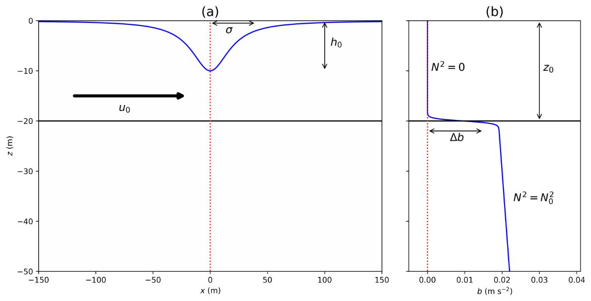
Figure 1 Schematic of sea ice keel moving relative to the ocean with (a) dimensions (width σ and maximum depth h₀) and speed of the ice keel relative to the ocean (u₀), and (b) vertical stratification of the underlying ocean (mixed layer depth z₀, density jump across the pycnocline Δb, and buoyancy frequency below the pycnocline N₀).

The forcing arises from the horizontal velocity of the drifting ice relative to the underlying ocean current, with components $(u,v)=(u_{\mathrm{ice}}-u_{\mathrm{ocean}},v_{\mathrm{ice}}-v_{\mathrm{ocean}})$. Combining the two velocity components, we define relative forcing magnitude to be $u_{\mathrm{0}}=\sqrt{u^{\mathrm{2}}+v^{\mathrm{2}}}$ (see Fig. 1a). The vertical stratification of the ocean is characterized as two layers: well-mixed layer of depth z₀ with zero buoyancy frequency N=0 separated by a sharp pycnocline with buoyancy jump Δb from the lower weakly stratified layer with buoyancy frequency N₀ (see Fig. 1b).

McPhee and Kantha (1989) derives the IW drag coefficient C_IW by finding analytical expressions for horizontal velocity $\stackrel{\mathrm{̃}}{u}$ and vertical velocity $\stackrel{\mathrm{̃}}{w}$ at the pycnocline and computing the wave radiation Reynolds stress:

$$\begin{array}{}\text{(3)}& \mathit{\tau }=\mathit{\rho }\stackrel{\mathrm{̃}}{u}\stackrel{\mathrm{̃}}{w}=\mathit{\rho }{C}_{\mathrm{IW}}{u_{\mathrm{0}}}^{\mathrm{2}}.\end{array}$$

Expressions for the velocities at the pycnocline $\stackrel{\mathrm{̃}}{u}$ and $\stackrel{\mathrm{̃}}{w}$ are derived by matching wave solutions in the mixed layer and the stratified interior at the interface. C_IW can then be expressed as the product of a drag coefficient for a fully stratified water column, C_DNW, and a damping factor Γ that depends on the buoyancy jump and mixed layer depth:

$$\begin{array}{}\text{(4)}& C_{\mathrm{IW}}=\mathrm{\Gamma }{C}_{\mathrm{DNW}}.\end{array}$$

The damping factor Γ accounts for the reduction of drag due to finite mixed-layer depth. The formulations for C_DNW and Γ given in McPhee and Kantha (1989) and Flocco et al. (2024) are written in terms of the six dimensional sea ice- and ocean-related variables:

$$\begin{array}{}\text{(5)}& \begin{array}{rl}& {\mathrm{\Gamma }}^{\dim }(u_{\mathrm{0}},N_{\mathrm{0}},k_{\mathrm{0}},z_{\mathrm{0}},\mathrm{\Delta }b)\\ & =(\mathrm{1}+\left({\displaystyle \frac{N_{\mathrm{0}}^{\mathrm{2}}}{u_{\mathrm{0}}^{\mathrm{2}}{k}_{\mathrm{0}}^{\mathrm{2}}}}+{\left({\displaystyle \frac{\mathrm{\Delta }b}{k_{\mathrm{0}}{u}_{\mathrm{0}}^{\mathrm{2}}}}\right)}^{\mathrm{2}}\right){\sinh }^{\mathrm{2}}(k_{\mathrm{0}}{z}_{\mathrm{0}})\\ & -{\displaystyle \frac{\mathrm{\Delta }b}{k_{\mathrm{0}}{u}_{\mathrm{0}}^{\mathrm{2}}}}\sinh \left(\mathrm{2}{k}_{\mathrm{0}}{z}_{\mathrm{0}}\right){)}^{-\mathrm{1}},\end{array}\end{array}$$

while the drag coefficient in a fully stratified (deep, non–mixed-layer) ocean is

$$\begin{array}{}\text{(6)}& C_{\mathrm{DNW}}^{\dim }(u_{\mathrm{0}},N_{\mathrm{0}},k_{\mathrm{0}},h_{\mathrm{0}})={\displaystyle \frac{k_{\mathrm{0}}{N}_{\mathrm{0}}{h}_{\mathrm{0}}^{\mathrm{2}}}{\mathrm{2}{u}_{\mathrm{0}}}}\sqrt{\mathrm{1}-{\left({\displaystyle \frac{u_{\mathrm{0}}{k}_{\mathrm{0}}}{N_{\mathrm{0}}}}\right)}^{\mathrm{2}}}.\end{array}$$

This formulation, implemented in a recent coupled ice–ocean model (Flocco et al., 2024), reflects how variations in keel geometry, current speed, stratification, and mixed layer depth combine to regulate the efficiency of momentum transfer from drifting ice keels into the ocean interior.

2.2 Nondimensionalization

Since these six dimensional quantities (u₀, h₀, k₀, z₀, Δb, and N₀) span different units and scales, it is more effective to describe the system in terms of four nondimensional ratios that capture the relative importance of keel geometry, velocity forcing, and ocean stratification. These nondimensional parameters reduce the number of free variables and provide a compact framework to identify dynamical regimes.

The first two nondimensional parameters following the classical flow-topography interaction theory are the lee wave radiation parameter χ defined in Eq. (1) and keel criticality parameter J defined in Eq. (2). The combination of these two nondimensional parameters is another nondimensional parameter that measures keel steepness:

$$\begin{array}{}\text{(7)}& \mathit{\zeta }={\displaystyle \frac{h_{\mathrm{0}}}{L/\mathrm{2}}}={\displaystyle \frac{h_{\mathrm{0}}{k}_{\mathrm{0}}}{\mathit{\pi }}}={\displaystyle \frac{\mathit{\chi }J}{\mathit{\pi }}}.\end{array}$$

Greater ζ corresponds steeper keel sides, i.e., to deeper and/or less wide keels. However, as it is not independent of the other nondimensional parameters, we will not explicitly use it in our analysis.

The third parameter is the depth ratio η, which quantifies how far the keel protrudes below the mixed layer:

$$\begin{array}{}\text{(8)}& \mathit{\eta }={\displaystyle \frac{z_{\mathrm{0}}}{h_{\mathrm{0}}}},\end{array}$$

The larger η is, the smaller the keel is compared to the mixed layer depth, and the larger the distance from the keel to the pycnocline. This would potentially limit the keel's ability to generate disturbance at the pycnocline and radiate IWs into the stratified interior.

The final parameter is the Froude number that compares kinetic energy of the forcing to the potential energy barrier of the pycnocline and is related to the Richardson number Ri in the McPhee and Kantha (1989) parameterization:

$$\begin{array}{}\text{(9)}& F{r}^{\mathrm{2}}={\displaystyle \frac{u_{\mathrm{0}}^{\mathrm{2}}{k}_{\mathrm{0}}}{\mathrm{\Delta }b}}={\displaystyle \frac{\mathrm{1}}{Ri}}\end{array}$$

Larger Fr (smaller Ri) corresponds to a weaker pycnocline and/or stronger forcing and has been previously found to result in more unstable, supercritical flow conditions (De Abreu et al., 2024).

We can then re-write the drag coefficient in the stratified interior $C_{\mathrm{DNW}}^{\dim }$ (Eq. 6) and the attenuation factor Γ^dim (Eq. 5) using these four nondimensional parameters, which will simplify our exploration and understanding of the parameter regimes:

$$\begin{array}{}\text{(10)}& {\displaystyle }\begin{array}{rl}\mathrm{\Gamma }(\mathit{\chi },J,\mathit{\eta },Fr)& =(\mathrm{1}+\left({\displaystyle \frac{\mathrm{1}}{{\mathit{\chi }}^{\mathrm{2}}}}+{\displaystyle \frac{\mathrm{1}}{F{r}^{\mathrm{4}}}}\right){\sinh }^{\mathrm{2}}(\mathit{\chi }J\mathit{\eta })\\ & -{\displaystyle \frac{\mathrm{1}}{F{r}^{\mathrm{2}}}}\sinh \left(\mathrm{2}\mathit{\chi }J\mathit{\eta }\right){)}^{-\mathrm{1}},\end{array}\text{(11)}& {\displaystyle }{C}_{\mathrm{DNW}}(\mathit{\chi },J)={\displaystyle \frac{\mathit{\chi }{J}^{\mathrm{2}}}{\mathrm{2}}}\sqrt{\mathrm{1}-{\mathit{\chi }}^{\mathrm{2}}}.\end{array}$$

3 Data and GMM Methodology

We use output from Flocco et al. (2024) based on the ocean model NEMO (Nucleus for European Modelling of the Ocean) version 3.6 (Storkey et al., 2018) coupled with sea ice model CICE version 5.1 (Hunke et al., 2010). The model is atmospherically forced using NCEP-DOE-2 Reanalyses data (Kanamitsu et al., 2002) over the 2000–2017 time period. The details of model set-up, implementation, and validation are in Flocco et al. (2024), Storkey et al. (2018), and Stroeve et al. (2018), which we summarize here. Specifically, we use the reference run from their study, in which the ice–ocean drag coefficient only includes form and skin drag contributions calculated using the parameterization from Tsamados et al. (2014) without the parameterized IW drag. The model has 1^∘ degree tripolar grid (approximately 40 km grid resolution). It has 75 unevenly-spaced layers in the vertical: 1 m spacing near the surface increasing to 2 m at 10 m depth and towards 200 m near the bottom, with 31 depth levels within the top 200 m aimed to resolved the near-surface processes. The timestep is 2700 s. Unresolved subgrid motions of the flow, i.e., the vertical mixing of tracers and momentum, are parameterized using turbulent kinetic energy (TKE) scheme (Storkey et al., 2018). The sea ice model CICE accounts for the deformation of the sea ice cover using an elastic anisotropic-plastic rheology model (Tsamados et al., 2013) and for thermodynamical processes through an energy-conserving thermodynamic model of sea ice (Bitz and Lipscomb, 1999) and a melt pond model (Flocco et al., 2010). The sea ice and ocean models are coupled through the parameterized quadratic form drag (Tsamados et al., 2014).

The resulting dataset contains monthly-mean relevant sea ice and ocean variables over the 18 year period. The model output is, of course, merely an approximation of the real ocean sea ice state, limited by modeling assumptions, e.g., resolution and parameterization of small-scale processes. However, the goal of this study is to identify sea ice parameter regimes and parameter value ranges to ultimately improve sea ice drag parameterizations in ocean models. Therefore, it is adequate for this study to use an output from a sea ice-ocean coupled model as a representative sample, but we discuss some implications of the modeling choices in the Flocco et al. (2024) study for the parameter values in Sect. 6.2.

For each monthly time step and horizontal grid cell (at given latitude and longitude) in the NEMOv3.6 and CICEv5.1 model output from Flocco et al. (2024), we first compute the four nondimensional parameters defined in Sect. 2.2 using the corresponding sea ice and ocean variables. Note that the ocean velocity to compute u₀ is taken just below the pycnocline. We then perform an initial filtering step to remove all samples (i.e., individual time–grid coordinate pairs) where the χ falls outside the lee wave radiating range $\mathrm{0}<\mathit{\chi }<\mathrm{1}$. For the total dataset, this excludes about 32 % of the data points. In the summer months (June-August, denoted throughout text as JJA), approximately 17 % of data points have x>1, and in the winter months (December–February, denoted throughout text as DJF), approximately 38 % of the data points have χ>1. In this regime, we would expect no significant IW drag, so most of the drag on the ice keels would be from form and skin drag. For each parameter, these filtered values are then averaged along the time dimension at every spatial grid point. We examine three separate time-averages: (1) annual-average, (2) average over the summer months (JJA), and (3) average over the winter months (DJF). Notably, our definition of the summer months, while common, omits September, when the Arctic sea ice extent and thickness are typically at their minimum, so we could be omitting some shallow pycnoclines and small keel depths from the summer analysis. The time-averaging collapses the temporal variability into a single representative statistic, producing one time-averaged value per parameter for each horizontal grid cell across the model domain. To further reduce the influence of extreme values, for each parameter, we remove spatial grid points whose value exceeded the 95th percentile of that parameter’s distribution, thereby reducing right-skewness and preventing a few extreme values from dominating the results. Filtering is applied in this way to predominantly exclude values with extremely large magnitudes. A grid cell was discarded if any of its parameter values fell outside its respective range. This two-stage filtering process produces three sets (one for each averaging period) of four time-averaged nondimensional parameters as shown in Fig. 2. The effects of the seasonal differences of the nondimensional parameters are discussed in Sect. 5.2.

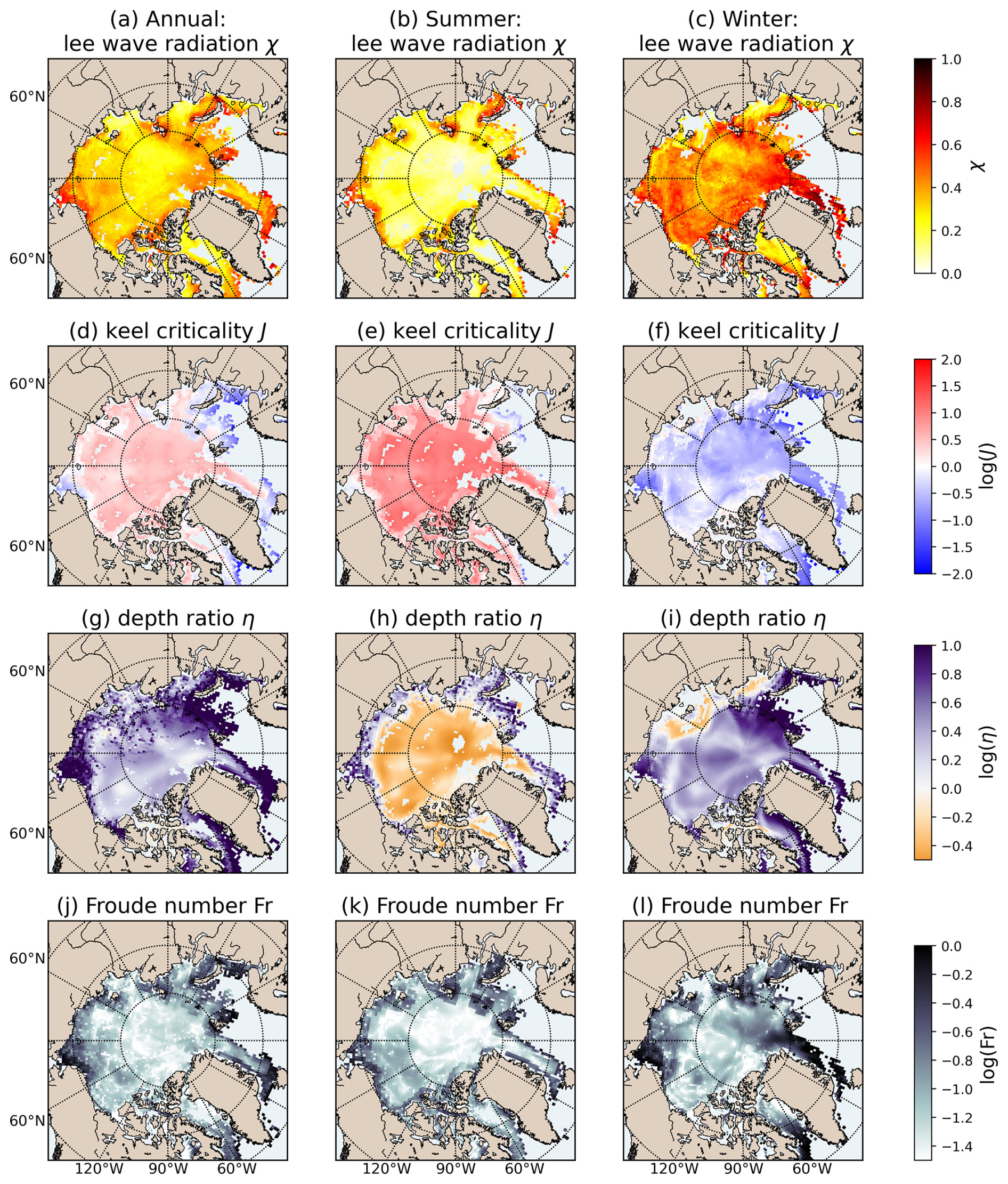
Figure 2 Spatial distribution of time-averaged four nondimensional parameters over the Arctic Ocean: (a–c) χ defined in Eq. (1), (d–f) J defined in Eq. (2), (g–i) η defined in Eq. (8), and (j–l) Fr defined in Eq. (9). Parameters are averaged over different time periods: (a, d, g, j) annually, (b, e, h, k) summer months (JJA), and (c, f, i, l) winter months (DJF). The post-processing of the variables is described in Sect. 3. Note that colorbars vary across subplots and the magnitudes of J, η and Fr are shown on a logarithmic scale. Figure is made with Matplotlib Basemap toolkit library (https://matplotlib.org/basemap/stable/, last access: 1 March 2026).

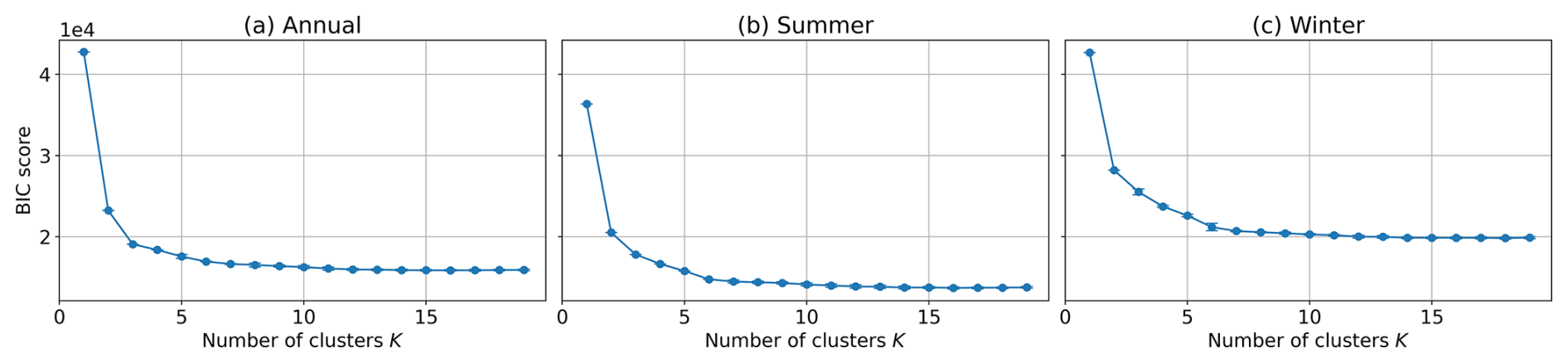
Figure 3 Bayesian Information Criterion (BIC) scores for GMM fitted to the four-dimensional feature space composed of χ, J, η, and Fr averaged (a) annually, (b) over summer months (JJA), and (c) over winter months (DJF). Models were fitted for cluster numbers ranging from 1 to 19. Each model fitting was repeated 20 times with different random initializations to assess variability in BIC values; error bars indicate ±1 standard deviation.

GMM is an unsupervised clustering algorithm, similar to K-means, which separates data points into K clusters in M-dimensional space. Here, M=4 because we have four nondimensional variables. GMM was chosen because, unlike the K-means algorithm, it accommodates elliptical cluster shapes and provides probabilistic membership assignments, allowing for uncertainty quantification in cluster classification. The number of clusters K is not known a priori and has to be determined using the Bayesian Information Criterion (BIC) as shown in Fig. 3. BIC score rewards higher probability of a data point belonging to one of the clusters, while punishing a large number of clusters. Therefore, one can run a parameter sweep selecting the configuration that minimized BIC across a tested range of the number of clusters K. In this paper, we choose K=6 because it is near the BIC curve's elbow point (Fig. 3) and offers a good balance between model simplicity and interpretability, which diminishes with too many clusters (Jones and Ito, 2019).

For each time-averaging period (annual, summer, winter), the GMM is fit to the entire dataset of nondimensional parameter values, treating each observation as an independent sample in the four‐dimensional parameter space. Cluster labels are then assigned to each observation based on the maximum posterior probability as shown in Fig. 4, and the corresponding spatial patterns of these clusters are analyzed to interpret the underlying physical regimes. We can also assess the performance of the GMM algorithm by evaluating the maximum posterior probability of the points assigned to each cluster as shown in Fig. 5. Values of posterior probability closer to unity indicate a high degree of confidence that the point belongs to that cluster. Most of the points in all clusters have large posterior probability values, and we find that almost all points within each cluster (more that 95 % of points) have posterior probability of greater than 0.5. This suggests that the clustering algorithm has distributed the samples with a relatively high degree of confidence. However, some of the larger clusters, e.g., clusters S0, S1, W0, and W1 (Fig. 5b, c, e, f), have patches with lower posterior probability, suggesting that they could be broken into smaller clusters. We will further discuss the implications of our choices for the number of clusters and analysis of the clustering algorithm performance in Sect. 6.2.

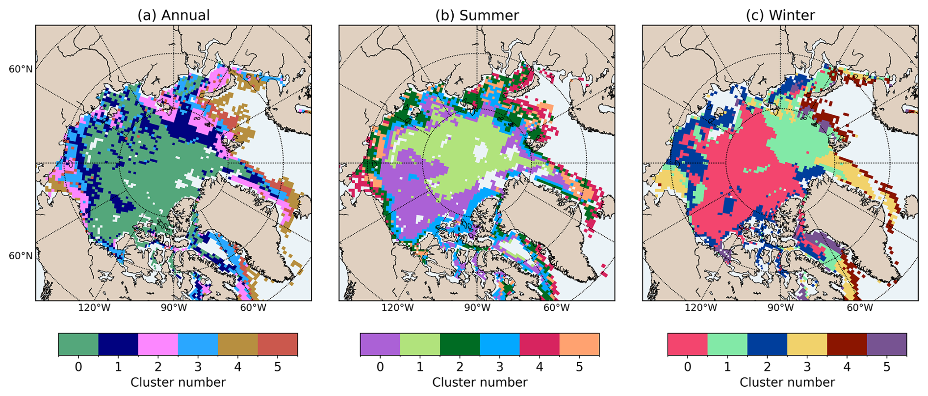
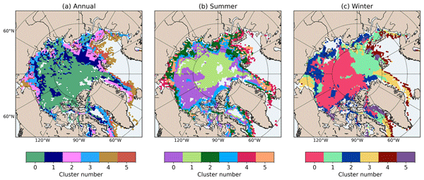
Figure 4 The spatial distribution of six statistically inferred regimes (K=6), each represented by a unique color, over the Arctic Ocean domain, derived from a GMM fitted to standardized time-averaged nondimensional parameter clusters across all spatial grid points. The values are based on the values averaged over different time intervals: (a) annually, (b) over the summer months (JJA), and (c) over the winter months (DJF). Clusters within each temporal averaging space are all ordered in the descending proportion of data points that belong to each cluster (i.e., most data points belong to cluster 0). Figure is made with Matplotlib Basemap toolkit library (https://matplotlib.org/basemap/stable/, last access: 1 March 2026).

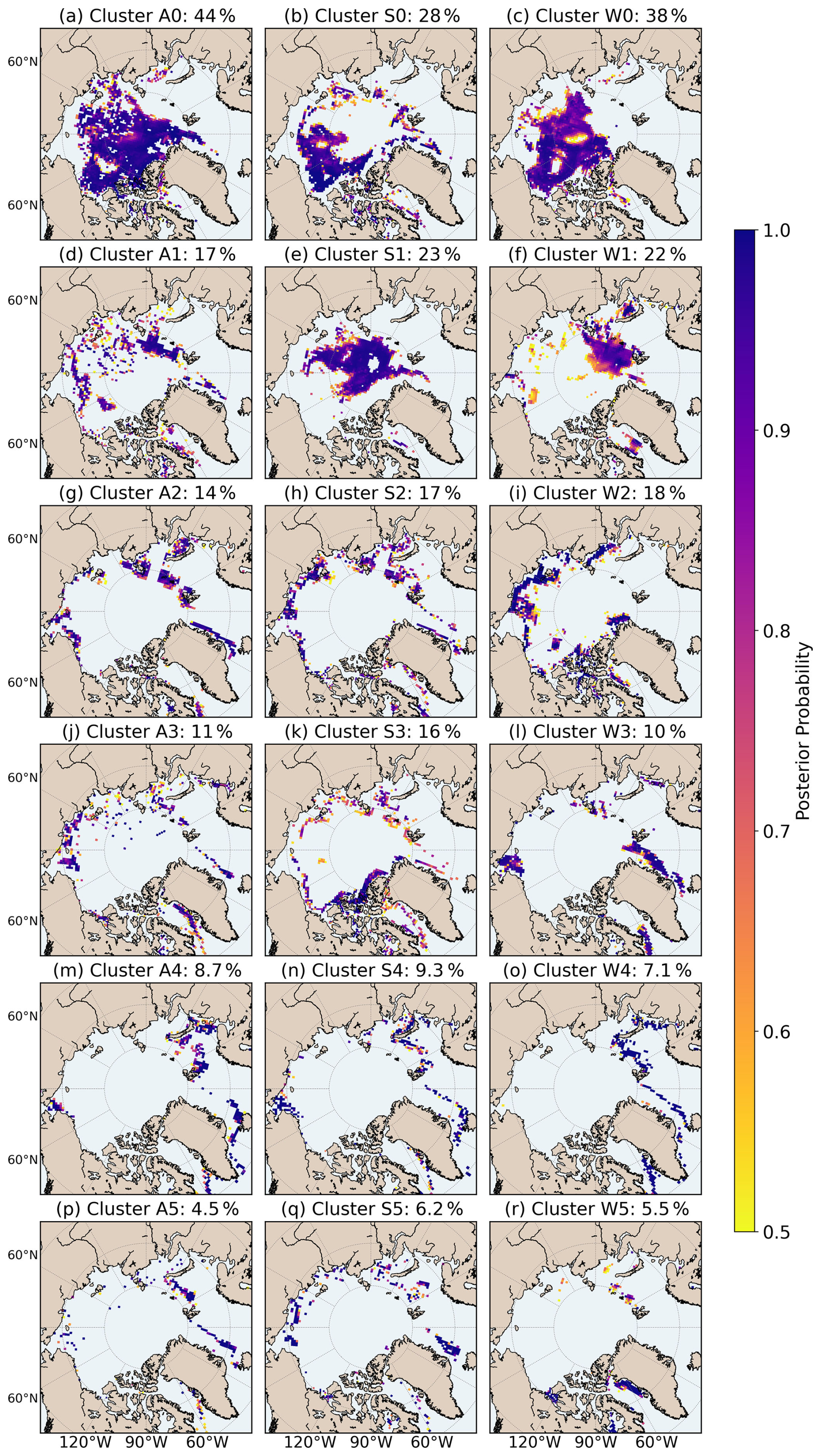
Figure 5 Posterior probability maps for each of the six clusters identified by the GMM, based on time-averaged standardized nondimensional parameters (χ, J, η, and Fr). The clusters are based on the values averaged over different time intervals: (left) annually “A”, (middle) summer (JJA) “S”, and (right) winter (DJF) “W”. Each subplot shows the posterior confidence that a given spatial grid cell belongs to the respective cluster. Clusters within each temporal averaging space are all ordered in the descending proportion of data points that belong to each cluster and the proportion is shown in each subplot title.

4 Numerical simulations

4.1 Set-up

In order to illustrate the differences in the dynamical regimes for each cluster identified by the GMM, we perform numerical simulations of the idealized problem shown in Fig. 1. Similar to previous studies (e.g., Zhang et al., 2022; De Abreu et al., 2024), our simulations are two-dimensional in (x,z). Technically, the domain is two-and-a-half dimensional with just one grid cell in the y-direction, and the velocity in the y-direction can be non-zero but all derivatives with respect to y are zero. Specifically, we solve the following non-hydrostatic rotating Navier-Stokes equations with the Boussinesq approximation:

$$\begin{array}{}\text{(12)}& {\displaystyle \frac{\partial \mathit{u}}{\partial t}}+\mathit{u}\cdot \mathrm{\nabla }\mathit{u}-\mathit{f}\times \mathit{u}=-{\displaystyle \frac{\mathrm{\nabla }p}{{\mathit{\rho }}_{\mathrm{0}}}}+\mathit{\nu }{\mathrm{\nabla }}^{\mathrm{2}}\mathit{u}+b\mathit{k}+f{u}_{\mathrm{0}}\mathit{j},\text{(13)}& {\displaystyle \frac{\partial b}{\partial t}}+\mathit{u}\cdot \mathrm{\nabla }b=\mathit{\kappa }{\mathrm{\nabla }}^{\mathrm{2}}b,\text{(14)}& {\displaystyle }\mathrm{\nabla }\cdot \mathit{u}=\mathrm{0},\end{array}$$

where $\mathit{u}=(u,v,w)$ is the velocity in $(x,y,z)$ directions, p is pressure, $b=-g(\mathit{\rho }-{\mathit{\rho }}_{\mathrm{0}})/{\mathit{\rho }}_{\mathrm{0}}$ is buoyancy for density $\mathit{\rho }(x,z,t)$ and constant reference density ρ₀, f=fj for local Coriolis parameter f, j and k are unit vectors in y and z directions, respectively, and ν and κ are kinematic viscosity and diffusivity, respectively. For steady velocity forcing, the term fu₀ is added to the y-momentum equation analogous to the simulations by Klymak (2018) and Zemskova and Grisouard (2021).

While the parameterization in McPhee and Kantha (1989) was derived for a sinusoidal ice keel shape, in more recent numerical studies (e.g., Skyllingstad et al., 2003; Zhang et al., 2022; De Abreu et al., 2024), it has been more common to model keel shape h(x) using a Versoria function

$$\begin{array}{}\text{(15)}& h\left(x\right)={\displaystyle \frac{h_{\mathrm{0}}{\mathit{\sigma }}^{\mathrm{2}}}{{\mathit{\sigma }}^{\mathrm{2}}+\mathrm{4}{x}^{\mathrm{2}}}},\end{array}$$

with width σ, which we also use in our numerical simulations as shown in the schematic in Fig. 1. However, the CICEv5.1 model output reports L rather than σ and theoretical nondimensional numbers are typically expressed in terms of k₀ (wavenumber of a sinusouidal keel), so we make the approximate connection that $\mathit{\sigma }=\mathit{\pi }/\left(\mathrm{2}{k}_{\mathrm{0}}\right)$.

The equations are solved using Oceananigans.jl (Ramadhan et al., 2020; Wagner et al., 2025) to take advantage of the enhanced computational speeds by GPUs (Silvestri et al., 2025). In its current implementation, an immersed boundary grid to model an obstacle (e.g., bottom topography or an ice keel) can only be specified along the bottom boundary. However, we can apply the property of the Boussinesq flows in that the flow is symmetric when flipped vertically, assuming that the buoyancy is also flipped in sign. That is, for example, in the Boussinesq approximation, cool dense water sinking and warm light water rising appear as vertically-flipped mirror images. Therefore, we model a flipped version of Fig. 1 by imposing a Versoria-shaped (Eq. 15) immersed boundary along the bottom of the domain and initializing the buoyancy profile as

$$\begin{array}{}\text{(16)}& \begin{array}{rl}& b_{\mathrm{0}}\left(z\right)\\ & ={\displaystyle \frac{\mathrm{1}}{\mathrm{2}}}\left(\mathrm{\Delta }b-{N_{\mathrm{0}}}^{\mathrm{2}}\left(-H-z_{\mathrm{0}}-z\right)\right)\left(\mathrm{1}-\tanh \left({\displaystyle \frac{-H-z_{\mathrm{0}}-z}{\mathit{\mu }}}\right)\right),\end{array}\end{array}$$

where H is the maximum depth of the domain and μ is the pycnocline width taken to be 0.5 m for all simulations. The width μ is taken to be a small finite value to represent a sharp pycnocline yet to maintain numerical stability of the simulations. However, it can also be varied after examining observational measurements of the stratification profiles in the Arctic, thus creating a fifth nondimensional parameter.

In order to avoid reflections off the top rigid-lid surface, we implement an exponential sponge layer $e^{-z^{\mathrm{2}}/\mathrm{2}{\mathit{\delta }}^{\mathrm{2}}}$ with $\mathit{\delta }=-H/\mathrm{20}$, which corresponds to the sponge layer being applied within approximately the top 20 m. Within the sponge layer, the flow is relaxed with a damping rate of $\mathrm{1}/\left(\mathrm{20}\mathrm{\Delta }t\right)$ to the initial conditions: b₀(z) for buoyancy, u₀ for u, and zero for w. In order to maintain numerical stability of the simulations, we take values for ν, κ, and Δt similar to those of De Abreu et al. (2024), namely, $\mathit{\nu }=\mathit{\kappa }={\mathrm{10}}^{-\mathrm{3}}$ m² s⁻¹ and $\mathrm{\Delta }t=\mathrm{6}\times {\mathrm{10}}^{-\mathrm{3}}$ s. However, unlike De Abreu et al. (2024), we do not apply sponge layers along the left and right boundaries, as these sponge layers were found to trigger artificial disturbances that travel downstream generating flow instabilities. Instead, we set the horizontal boundaries to be periodic and run the simulations for 6 h, which we found to be enough time for the flow to reach a quasi-steady state, but not enough time for the instabilities re-entering the domain through the periodic boundaries to reach the topographic obstacle. Finally, we set $f=\mathrm{1.36}\times {\mathrm{10}}^{-\mathrm{4}}$ s⁻¹ corresponding to 70° N, though rotation is not likely to significantly influence the simulations as the total length of the simulation time is less than one inertial period (≈12.8 h).

The domain for all numerical simulations is $x\in [-L_x/\mathrm{2},L_x/\mathrm{2}]$ for L_x=1200 m and $z\in [-H,\mathrm{0}]$ with H varying depending on the mixed layer depth for the simulation (see Table 1). For all simulations, we set u₀=0.1 m s⁻¹ and width of the Versoria-shaped obstacle (i.e., ice keel) as in Eq. (15) to be σ=40 m. Recall that $k_{\mathrm{0}}=\mathit{\pi }/\mathrm{2}\mathit{\sigma }$. We then compute all other dimensional parameters using the nondimensional parameter values as:

$$\begin{array}{}\text{(17)}& N_{\mathrm{0}}={\displaystyle \frac{u_{\mathrm{0}}{k}_{\mathrm{0}}}{\mathit{\chi }}},\mathrm{\Delta }b={\displaystyle \frac{k_{\mathrm{0}}{u}_{\mathrm{0}}^{\mathrm{2}}}{F{r}^{\mathrm{2}}}},h_{\mathrm{0}}={\displaystyle \frac{\mathit{\chi }J}{k_{\mathrm{0}}}},\mathrm{and}{z}_{\mathrm{0}}=-\mathit{\eta }{h}_{\mathrm{0}}.\end{array}$$

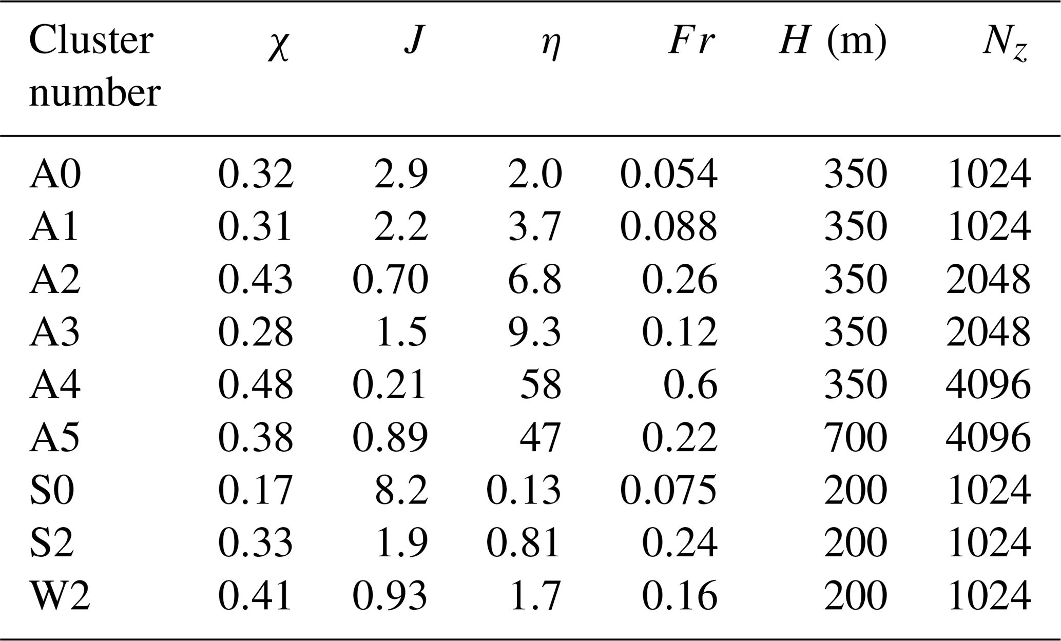
We perform nine numerical simulations: one for each of the annually-averaged clusters A0–5 and additionally for two summer clusters (S0 and S2) and one winter cluster (W2). The additional clusters are selected based on relatively large predicted C_IW from the parameterizations as will be shown in Sect. 5.2. These additional clusters also allow us to investigate the parameter regime were the ice keel protrudes below the mixed layer depth, i.e., η<1 (h₀>z₀), or the keel depth is close to the mixed layer depth, i.e., η∼1 (h₀∼z₀), which is not represented by the mean values of clusters A0–5. The numerical simulations are set up taking the mean nondimensional parameter values χ, J, η, and Fr for each of the GMM clusters. These values are summarized in Table 1 and are further discussed in Sect. 5. The horizontal resolution is the same for all simulations (N_x=4096 grid points), but the vertical resolution varies to allow approximately the same number of points within keel height h₀ as shown in Table 1.

Table 1 Mean values of each of the four nondimensional parameters, simulation domain depth H, and vertical number of discretization points N_z for each of the numerical simulations performed in this study (A0–5, S0, S2, W2) described in Sect. 4.. The extent of each cluster is shown in Fig. 4. The nondimensional variables are defined in text: χ in Eq. (1), J in Eq. (2), η in Eq. (8), and Fr in Eq. (9).

4.2 Analysis metrics

To minimize the influence of the flow re-entering through periodic boundary conditions on the interpretation of our results, we limit the horizontal extent of the region of analysis for numerical simulations to $x\in [-\mathrm{200},\mathrm{200}]$ m. All horizontal averages and integrals are performed only within these bounds. Also, in order to be consistent with the orientation of ice keel being at the surface (rather than along the bottom as in the numerical simulation set-up), all of the subsequent equations and figures will be shown in terms of $\widehat{z}=-H-z$.

In order to compare the flow dynamics across the numerical simulations with different parameter regimes, we compute the fluctuating kinetic energy

$$\begin{array}{}\text{(18)}& E_{\mathrm{K}}(x,\widehat{z})={\displaystyle \frac{\mathrm{1}}{\mathrm{2}}}\left(u^{\prime }(x,\widehat{z}{)}^{\mathrm{2}}+w(x,\widehat{z}{)}^{\mathrm{2}}\right)\end{array}$$

and fluctuating kinetic energy dissipation

$$\begin{array}{}\text{(19)}& {\mathit{ϵ}}_{\mathrm{K}}(x,\widehat{z})=\mathit{\nu }\left({\left({\displaystyle \frac{\partial u^{\prime }}{\partial x}}\right)}^{\mathrm{2}}+{\left({\displaystyle \frac{\partial u^{\prime }}{\partial \widehat{z}}}\right)}^{\mathrm{2}}+{\left({\displaystyle \frac{\partial w}{\partial x}}\right)}^{\mathrm{2}}+{\left({\displaystyle \frac{\partial w}{\partial \widehat{z}}}\right)}^{\mathrm{2}}\right),\end{array}$$

where $u^{\prime }(x,\widehat{z})=u(x,\widehat{z})-u_{\mathrm{0}}$ is the velocity of fluctuations defined as the deviation of horizontal velocity u from the background u₀. This is a common way to define perturbations and compute fluctuating (or turbulent) kinetic energy budget terms in numerical simulations involving internal waves (e.g., Nikurashin and Ferrari, 2010b; Shakespeare and McC. Hogg, 2018; De Abreu and Timmermans, 2026). Note that in this definition of fluctuating kinetic energy budget terms, we include both the internal waves and smaller scale motions.

We then compute the area-averaged integrals of E_K and ϵ_K in three different vertical regions to understand the effects of the different parameter regimes on the flow. The first region denoted by subscript pyc is around the pycnocline, which we define to be z₀±10 m, and the integral is notationally expressed as

$$\begin{array}{}\text{(20)}& {〈\cdot 〉}_{\mathrm{pyc}}={\displaystyle \frac{\mathrm{1}}{A_{\mathrm{pyc}}}}\underset{-\mathrm{200}}{\overset{\mathrm{200}}{\int }}\underset{z_{\mathrm{0}}-\mathrm{10}}{\overset{z_{\mathrm{0}}+\mathrm{10}}{\int }}\cdot \mathrm{d}\widehat{z}\mathrm{d}x.\end{array}$$

The second region denoted by subscript above is above the pycnocline, that is between the pycnocline and the ice keel, i.e.,

$$\begin{array}{}\text{(21)}& {〈\cdot 〉}_{\mathrm{above}}={\displaystyle \frac{\mathrm{1}}{A_{\mathrm{above}}}}\underset{-\mathrm{200}}{\overset{\mathrm{200}}{\int }}\underset{z_{\mathrm{0}}+\mathrm{10}}{\overset{-h_{\mathrm{0}}/\mathrm{3}}{\int }}\cdot \mathrm{d}\widehat{z}\mathrm{d}x.\end{array}$$

The upper bound is taken to be $\widehat{z}=-h_{\mathrm{0}}/\mathrm{3}$ to exclude numerical boundary layer effects due to the immersed grid. The third region denoted by subscript below is below the pycnocline, i.e.,

$$\begin{array}{}\text{(22)}& {〈\cdot 〉}_{\mathrm{below}}={\displaystyle \frac{\mathrm{1}}{A_{\mathrm{below}}}}\underset{-\mathrm{200}}{\overset{\mathrm{200}}{\int }}\underset{-H+\mathrm{50}}{\overset{z_{\mathrm{0}}-\mathrm{10}}{\int }}\cdot \mathrm{d}\widehat{z}\mathrm{d}x.\end{array}$$

The lower bound is taken to be $\widehat{z}=-H+\mathrm{50}$ m to exclude the sponge layer. In Eqs. (20)–(22), A_pyc, A_above, and A_below are areas of each respective region. We report values that are time-averaged over the last hour of the simulation to account for any small-scale temporal fluctuations.

We expect that most of the influence of the ice keel on the flow will be confined within the mixed layer, i.e., above the pycnocline. As we aim to quantify the relative influence of the ice keel on the pycnocline and the stratified interior of the ocean below the pycnocline, for each simulation we also compute the ratios:

$$\begin{array}{}\text{(23)}& {\displaystyle \frac{{〈E_{\mathrm{K}}〉}_{\mathrm{above}}}{{〈E_{\mathrm{K}}〉}_{\mathrm{below}}}},{\displaystyle \frac{{〈{\mathit{ϵ}}_{\mathrm{K}}〉}_{\mathrm{above}}}{{〈{\mathit{ϵ}}_{\mathrm{K}}〉}_{\mathrm{below}}}},{\displaystyle \frac{{〈E_{\mathrm{K}}〉}_{\mathrm{above}}}{{〈E_{\mathrm{K}}〉}_{\mathrm{pyc}}}},{\displaystyle \frac{{〈{\mathit{ϵ}}_{\mathrm{K}}〉}_{\mathrm{above}}}{{〈{\mathit{ϵ}}_{\mathrm{K}}〉}_{\mathrm{pyc}}}}.\end{array}$$

The smaller magnitudes of these ratios indicate greater effects of the keel on the energy propagation and dissipation within the pycnocline region and below the pycnocline.

5 Results

5.1 Annual-mean cluster parameter regimes and flow characteristics

We first focus on the GMM clusters identified based on the annually-averaged data identifying their geographical extents and discussing differences in flow characteristics below the sea ice based on the illustrative numerical simulation results. Figure 4a shows these six clusters within the Arctic region identified by applying GMM to four time-averaged nondimensional parameters. Each cluster reflects different oceanographic and sea ice conditions as will be discussed below. These clusters exhibit coherent geographic patterns despite latitude and longitude not being used as input variables for the clustering.

Before discussing the nondimensional parameter regimes for each of the clusters, we first put their geographical distributions in perspective using the Arctic clusters derived by Simon et al. (2025) based on the spatio-temporal patterns of sea ice concentration (SIC) observations over the 1979–2023 time period. This previous study categorized the Arctic based on the seasonal SIC cycle into three categories: permanent sea ice cover (fully ice covered in winter and minimum of 70 % SIC in the summer), full winter cover (mostly ice-free in the summer), and partial winter cover (maximum 70 % SIC in the winter and ice-free in the summer). Cluster A0, which is the largest cluster (Fig. 5a), occupies the central Arctic basin. This cluster mostly corresponds to the region in Simon et al. (2025) characterized by permanent sea ice cover consistently throughout their time period of consideration. Cluster A1 (Fig. 5d) extends outward from Cluster A0. Comparing its spatial extent with the analysis by Simon et al. (2025), this region is still mostly within parts of the Arctic that are permanently covered by sea ice but undergoing temporal shifts in the seasonal SIC cycle. Clusters A2 (Fig. 5g) and A3 (Fig. 5j) predominantly correspond to the full winter sea ice cover regions (Simon et al., 2025), with A2 covering mostly outer parts of the Eurasian basin of the central Arctic and A3 occupying coastal regions. Finally, the smallest clusters A4 and A5 (Fig. 5m, p) occupy boundary regions falling predominantly within the partial winter sea ice cover regions identified by Simon et al. (2025).

Now that we have identified the geographic patterns of each of the clusters, we will compare the nondimensional parameter regimes associated with each cluster. The distributions of each of the nondimensional parameters separated by the GMM cluster are shown in the left column of Fig. 6. In this subsection, we will focus on the mean values of the nondimensional parameters for each cluster (Table 1) and discuss the dynamics of the different parameter regimes supported by the numerical simulations results. Snapshots of the flow fields for the numerical simulations are shown in Figs. 7–8 and the energetics metrics are summarized in Tables 2-3.

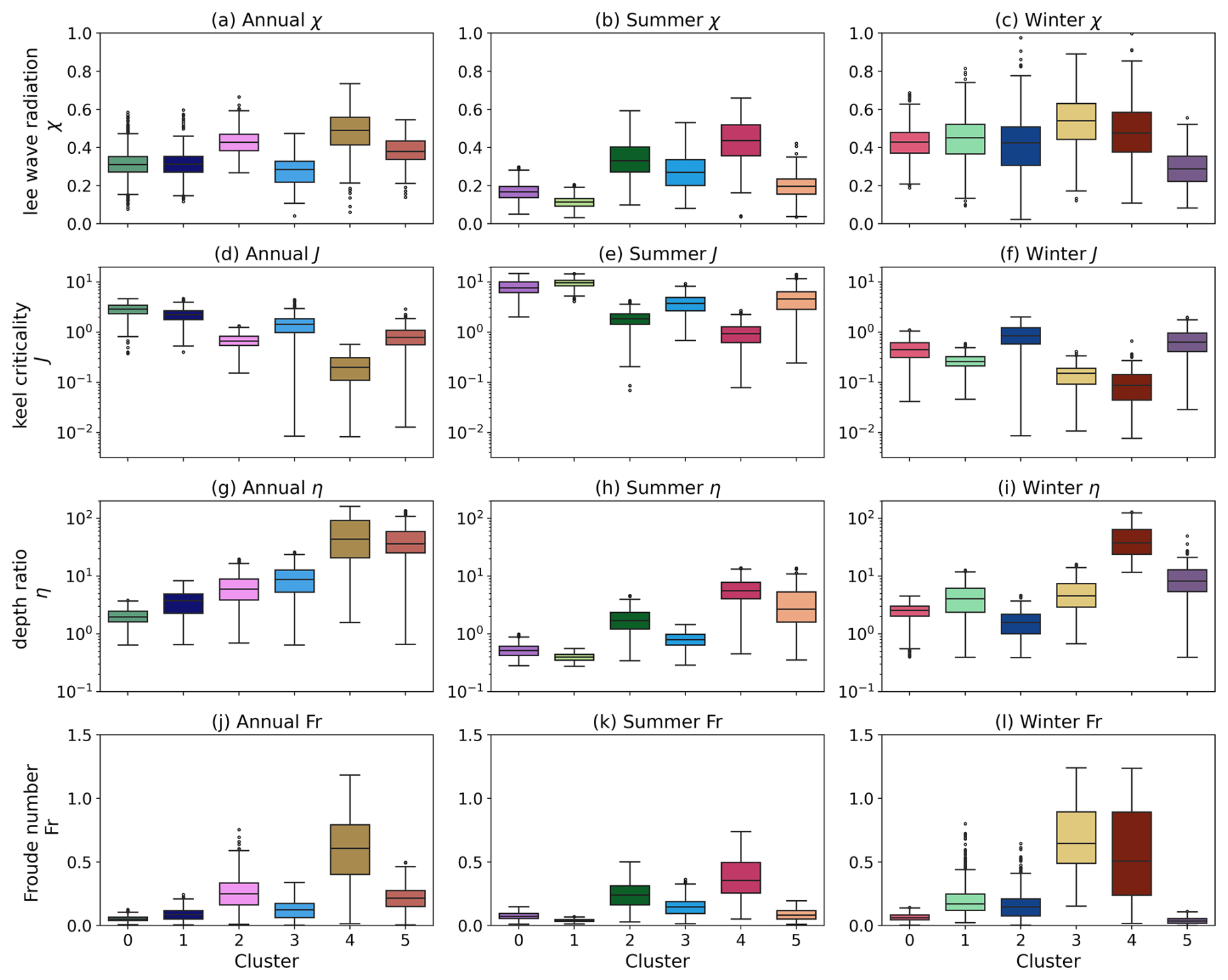
Figure 6 Distribution of nondimensional variables across six GMM clusters for different averaging periods: (a, d, g, j) annual, (b, e, h, k) summer months (JJA), and (c, f, i, l) winter months (DJF). For each averaging period, the spatial distributions of the clusters are shown in Fig. 4. Each subplot corresponds to a single parameter: (a–c) χ, (d–f) J, (g–i) η, and (j–l) Fr. Individual boxes show the interquartile range, median, and outliers for each cluster. Note that keel criticality parameter J (d–f) and depth ratio η (g–i) are plotted on a log scale to easily compare across clusters and seasons.

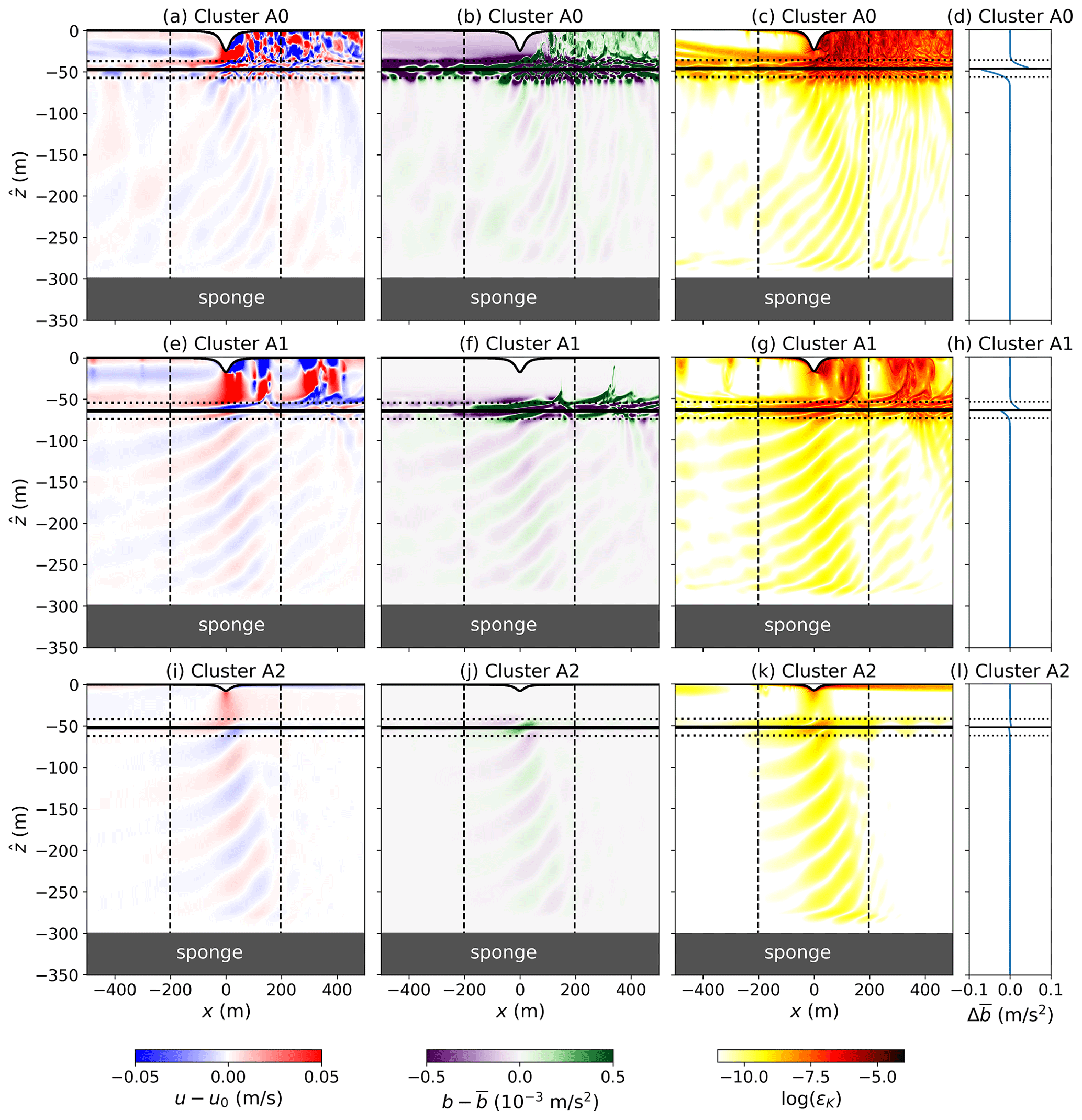
Figure 7 Snapshots from numerical simulations set with nondimensional parameters for GMM clusters (a–d) A0, (e–h) A1, and (i–l) A2: (a, e) turbulent horizontal velocity u−u₀, (b, f) buoyancy perturbations, i.e., deviations from horizontally-averaged $\stackrel{\mathrm{‾}}{b}\left(z\right)$, (c, g) log of kinetic energy dissipation ϵ_K, and (d, h) buoyancy deviation from initial conditions $\mathrm{\Delta }\stackrel{\mathrm{‾}}{b}=\stackrel{\mathrm{‾}}{b}\left(z\right)-b_{\mathrm{0}}\left(z\right)$. The thick black horizontal black lines in each subplot indicate the pycnocline $\widehat{z}=z_{\mathrm{0}}$ and horizontal dotted lines delineate $\widehat{z}=z_{\mathrm{0}}\pm \mathrm{10}$ m. In (a)–(c), (e)–(g), and (i)–(k), dashed vertical lines delineate the region $x\in [-\mathrm{200},\mathrm{200}]$ m, which is used for horizontal averages and integrals. All snapshots are for the last timestep (after 6 h) of simulation time.

Figure 8 Same as Figure 7 but for (a–d) Cluster A3, (e–h) Cluster A4, and (i–d) Cluster A5. Note that the colorbar in (b), (f), (j) for the buoyancy plots are different from those in Fig. 7.

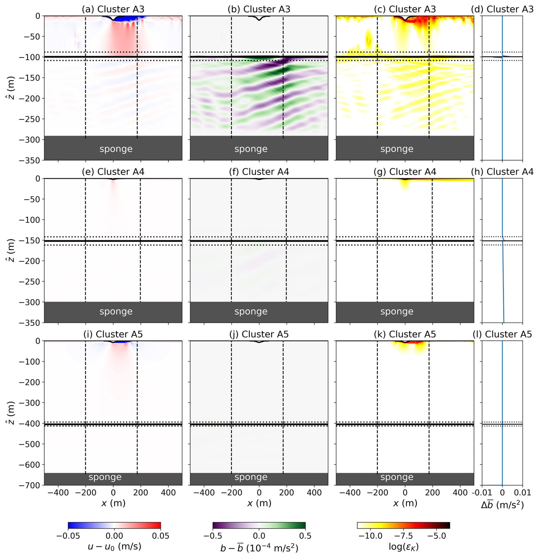
Table 2 Area-averaged turbulent kinetic energy E_K and turbulent kinetic energy dissipation ϵ_K averaged over the last hour of each numerical simulation. The regions of the simulation domain (within the pycnocline pyc, above the pycnocline above, and below the pycnoline below) are defined in Eqs. (20)-(22). The units for 〈E_K〉 terms are m² s⁻² and for 〈ϵ_K〉 terms are m² s⁻³. For simulations S0 and S2, values above the pycnocline are not computed because the mixed layer depth is too shallow (<15 m).

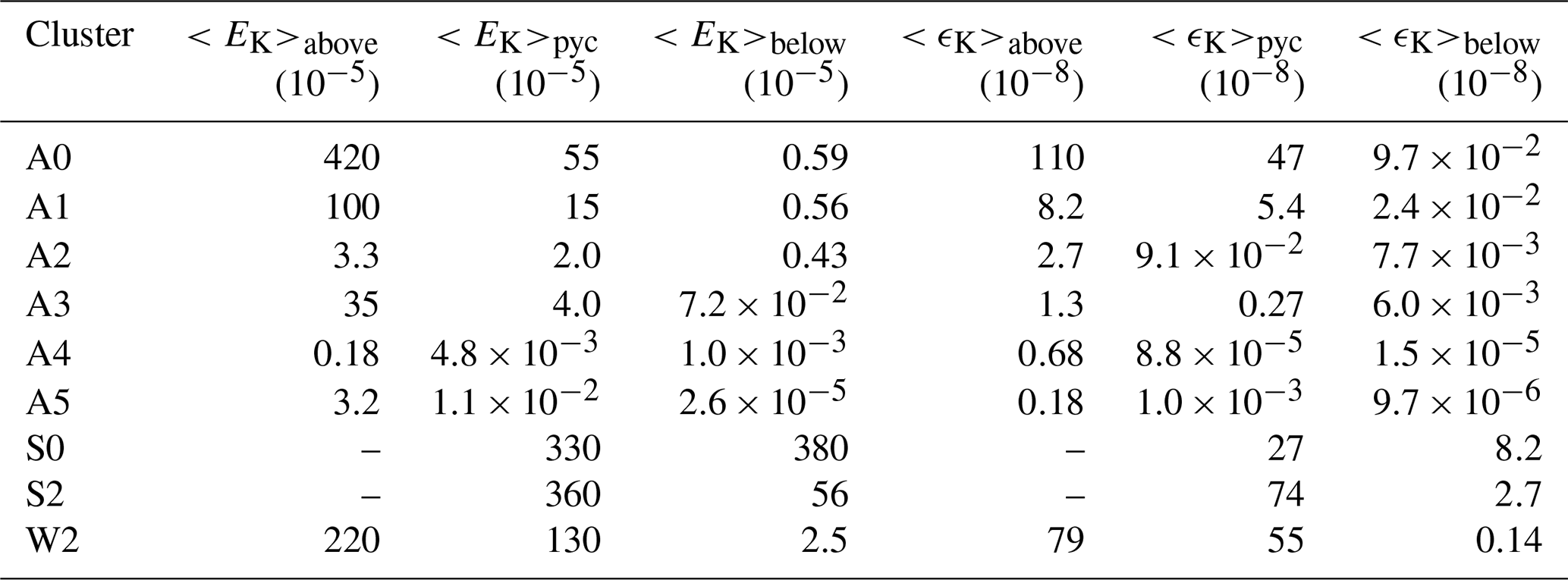
Table 3 Ratios of kinetic energy metrics to estimate the relative effects of the ice keel on the pycnocline and stratified interior below the pycnocline in each numerical simulation. Area-averaged turbulent kinetic energy E_K and turbulent kinetic energy dissipation ϵ_K averaged over the last hour of each numerical simulation. The regions of the simulation domain (within the pycnocline pyc, above the pycnocline above, and below the pycnoline below) are defined in Eqs. (20)–(22). S0 and S2 are omitted because for those two simulations, values above the pycnocline are not computed because the mixed layer depth is too shallow (<15 m).

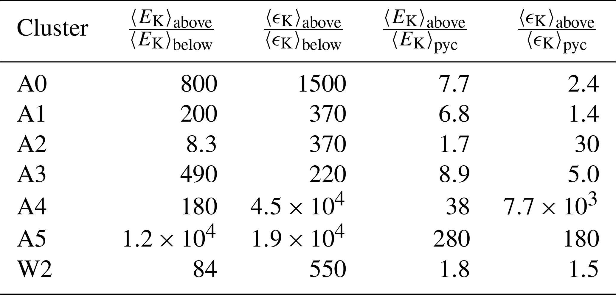
Broadly speaking, the central Arctic clusters A0 and A1 that fall within the permanent sea ice cover regions are characterized by relatively small values of depth ratio η (Fig. 6g) and Froude number Fr (Fig. 6j) and large values of keel criticality J (Fig. 6d). Large values of J and small values of η indicate that keels in this region possess strong potential to overcome stratification and drive vertical mixing. In the numerical simulations, we find large turbulent velocities (Fig. 7a, e) and dissipation rates (Fig. 7c, g), in particular above the pycnocline. Out of the six annual clusters, we find the largest amount of kinetic energy and dissipation rates in all parts of the domain (above, below, and within the pycnocline) for these two clusters (Table 2). The stratification in the vicinity of the pycnocline is also perturbed with evidence of small-scale turbulent motions, and the deviation from the initial stratification $\mathrm{\Delta }\stackrel{\mathrm{‾}}{b}$ is the largest across all simulations (Fig. 7b, d, f, h). However, the small Fr values reflect strong density stratification, which may suppress sustained turbulence and limit mixing to localized, shear-driven interfaces. We find energy propagation below the pycnocline into the stratified interior to be small (large values of ${〈E_{\mathrm{K}}〉}_{\mathrm{above}}/{〈E_{\mathrm{K}}〉}_{\mathrm{below}}$ and ${〈{\mathit{ϵ}}_{\mathrm{K}}〉}_{\mathrm{above}}/{〈{\mathit{ϵ}}_{\mathrm{K}}〉}_{\mathrm{below}}$ in Table 3). This suggests that the large value of density jump across the pycnocline (small Fr) can inhibit the effect of the ice keel despite the small value of η (so keel depth is the largest relative to mixed layer depth in comparison to other clusters). Comparing the two clusters, cluster A1 has smaller J and larger η than cluster A0. As a result, despite having larger value of Fr and thus smaller potential energy barrier at the pycnocline, the keel is less likely to reach or perturb the pycnocline, reducing mechanical coupling compared with cluster A0, thus smaller amount of kinetic energy and dissipation rates. However, because of a smaller density jump across the pycnocline (larger Fr), the lee-wave signature below the pycnocline is more coherent and the relative energy propagation below the pycnocline is larger (smaller values of ${〈E_{\mathrm{K}}〉}_{\mathrm{above}}/{〈E_{\mathrm{K}}〉}_{\mathrm{below}}$ and ${〈{\mathit{ϵ}}_{\mathrm{K}}〉}_{\mathrm{above}}/{〈{\mathit{ϵ}}_{\mathrm{K}}〉}_{\mathrm{below}}$) compared to cluster A0.

Cluster A2 continues this trend moving away from the Central Arctic Ocean towards parts of the Arctic that are only fully ice-covered in the winter with smaller keel criticality J and larger depth ratio η and Froude number Fr, pointing to a weaker pycnocline and greater susceptibility to intermittent IW activity below the pycnocline. It also has larger values of lee wave radiation parameter χ in comparison to the other Central Arctic Ocean clusters. The numerical simulations show overall smaller magnitude E_K and ϵ_K and less turbulent motions around the pycnocline (Fig. 7i–l) compared to central Arctic clusters A0–1 simulations, most likely due to smaller J (reduced nonlinearity of the flow) and larger η (small keel compared to mixed layer depth). However, because of larger Fr, wave energy propagation into the stratified interior below the pycnocline is larger (smaller ${〈E_{\mathrm{K}}〉}_{\mathrm{above}}/{〈E_{\mathrm{K}}〉}_{\mathrm{below}}$) in comparison to clusters A0–1.

Cluster A3 exhibits a blend of characteristics: keel criticality J larger than that of A2 suggesting some nonlinear flow motions, and intermediate stratification strength with Fr smaller than that of A2 but larger than those of A0–1, and depth ratio η larger in comparison to the central Arctic clusters A0–2 and smaller in comparison to marginal ice clusters A4–5. These conditions suggest lee wave generation and intermittent mixing, likely governed by the interplay between moderate mechanical forcing and stratification. Indeed, we find lee waves radiating below the pycnocline in the numerical simulations for this regime (Fig. 7i–l). While E_K and ϵ_K are smaller in magnitude in comparison with those for clusters A0–2, kinetic energy around the pycnocline ${〈E_{\mathrm{K}}〉}_{\mathrm{pyc}}$ and above the pycnocline ${〈E_{\mathrm{K}}〉}_{\mathrm{above}}$ is relatively large (Table 2). The dissipation within the pycnocline region is relatively small (larger value of ${〈{\mathit{ϵ}}_{\mathrm{K}}〉}_{\mathrm{above}}/{〈{\mathit{ϵ}}_{\mathrm{K}}〉}_{\mathrm{pyc}}$) possibly due to smaller Froude number (or stronger pycnocline).

Clusters A4–5 represent boundary or transitional regimes characterized by large values of η, i.e., a much deeper mixed layer in comparison to the keel depth (Fig. 6g). Data points within cluster A4 have more extreme or distinctive parameter values (e.g., largest mean Fr and χ and smallest mean J) and the largest variability within the cluster. We find that the ice keel has negligible effect on the flow for these parameter regimes (Fig. 8e–l). Both E_K and ϵ_K are smaller by at least 2–3 orders of magnitude in the numerical simulations for these clusters compared with the other clusters (Table 2) as wave propagation is getting suppressed by the deep pycnocline. The only notable exception is that 〈E_K〉 above the pycnocline is larger cluster A5 simulation than that of cluster A4 simulation and comparable to that of cluster A2, most likely due to a steeper keel (larger keel criticality J).

The numerical simulations presented here do not exhaustively capture the variability in the dynamical regimes and are primarily for illustrative purposes. However, through these simulations, we can already observe how differences in the nondimensional parameters change the flow characteristics, IW generation, propagation, and dissipation. For example, in general, we find that the amount of fluctuating KE and KE dissipation increases with increasing J (steeper keels, increased nonlinearity of the flow) and decreases with increasing η (keel further away from the pycnocline) with more complicated correlations with χ and Fr, though these relationships will need to be investigated thoroughly with a more comprehensive parameter sweep.

5.2 Seasonal variability of nondimensional parameters and internal wave drag estimates

While in the previous section we explored specific combinations of parameter values associated with each cluster in order to qualitatively assess their effects on the flow, in this section, we consider the spatial and seasonal variability of the nondimensional parameters in order to identify the ranges of values that are relevant to the sea ice keels. We then explore how this variability translates to the variability of IW drag values estimated from the McPhee and Kantha (1989) parameterization in Eqs. (10)–(11).

Seasonal differences between the summer- and winter-averaged distributions of the nondimensional parameters are shown in Fig. 2. Winter months are characterized by larger values of lee wave radiation parameter χ due to larger relative ice keel speeds u₀, especially in the Eurasian basin (Fig. S1b, c in the Supplement), and smaller buoyancy frequency N₀ in the stratified interior throughout most of the Arctic (Fig. S1h, i). Smaller N₀ and larger u₀ in the winter than in the summer also yields smaller keel criticality values: over most of the Arctic, J<1 in the winter and J>1 in the summer (Fig. 2e, f). The seasonal differences in the depth ratio η are mostly due to the differences in the mixed layer depth z₀ (Fig. S1n, o) rather than the keep depth h₀ (Fig. S1k, l). From these estimates, we find η<1 (mixed layer depth shallower than the keel depth) for most of the Arctic in the summer (Fig. 2h) and η>1 (z₀>h₀) in the winter (Fig. 2i). Froude number Fr is larger during the winter months in comparison to the summer (Fig. 2k, l), with particularly larger in the Eurasian Basin in the winter. This is due to smaller buoyancy jump across the pycnocline Δb in the winter (Fig. S1q, r) and larger relative keel speeds in the winter (Fig. S1b, c). Interestingly, the seasonal differences in the keel horizontal wavenumber k₀ (Fig. S1e, f) are not strongly reflected in the seasonal differences of the nondimensional parameters. Overall, k₀ is smaller in the winter, which would make χ and Fr smaller in the winter, but we do not find that to be the case.

The spatial distribution of GMM clusters also highlights the seasonal differences in nondimensional parameters (Figs. 4–5). For the annually-averaged data, the largest cluster A0 (40 % of data points, Fig. 5a) encompasses most of the central Arctic. In contrast, for the summer- and winter-averaged data, the central Arctic is more evenly and clearly divided into the Amerasian (S0 in Fig. 5b and W0 in Fig. 5c) and Eurasian (S1 in Fig. 5h and W1 in Fig. 5f) basins. In both basins, the values of χ, η, and Fr are overall smaller and the values of J are larger in the summer than in the winter. The nondimensional parameter ranges are different between these clusters and the inter-cluster differences vary across seasons. For example, in the winter months, we find larger values of J, η, and Fr (Fig. 6f, i, l) in the Eurasian basin than in the Amerasian basin, but the opposite to be the case in the summer months.

As captured by the IW drag parameterization in Eqs. (10)–(11) and observed based on the kinetic energy metrics in Sect. 5.1, the effects of the nondimensional parameters on these quantities is nonlinear. To explore whether IWs might play an important role in certain parts of the Arctic, we plot in Figure 9 the pair-wise distributions of nondimensional parameters χ, J, η, and Fr calculated based on ice keel and ocean variables averaged annually (first column from the left), over the summer months (second column from the left), and over the winter months (third column from the left). Ultimately, we wish to perform numerical simulations with parameter sweeps over these nondimensional parameters to test parameterization schemes included in regional and large-scale models, so it is important to limit the range of values for such sweeps. The pairwise distributions help us identify combinations of parameter values that might not need to be as thoroughly explored, e.g., combinations of (i) large χ and large J (Fig. 9a–c), (ii) large J and large η, and (iii) large J and large Fr. Furthermore, the breakdown of the pairwise distributions into the GMM clusters helps us identify combinations of nondimensional parameter values that, while present in the Arctic, might be less ubiquitous. For example, clusters A4, A5, and W4 show a high variability with respect to values of η and Fr (Fig. 6g, i, j, l), but each of them contains less that 15 % of all the data points in the Arctic (Fig. 5m, o, p). Therefore, even though the pairwise distribution shows values over the full range of η−Fr space (Fig. 9u, w), we find that most of the points (possibly over 85 %) have smaller values of η (≲10) and Fr (≲0.5).

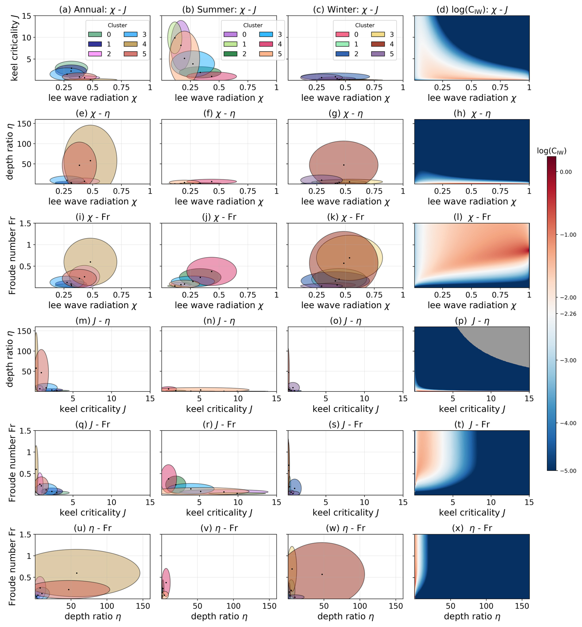
Figure 9 (left three columns) Pairwise ellipse plots showing the cluster-mean values and associated variability across six GMM-identified regimes (columns from left to right: Annual, Summer (JJA), Winter (DJF)). Each colored ellipse is centered at the cluster mean for the variable pair shown and spans two standard deviations along each axis, capturing the internal spread of that cluster. (right column) internal wave drag C_IW induced by the ice keel calculated from the parameterization expression over the joint pairwise parameter range. The values of C_IW are plotted on a logarithmic scale and the white values (center of the colorbar) corresponds to the canonical ice-ocean drag coefficient value of $C_{\mathrm{D}}=\mathrm{5.5}\times {\mathrm{10}}^{-\mathrm{3}}$ ($\log \left(C_{\mathrm{D}}\right)=-\mathrm{2.26})$. Subplots on each row correspond to the following pairs: (a–d) χ–J, (b–h) χ–η, (i–l) χ–Fr, (m–p) J–η, (q–t) J–Fr, and (u–x) η–Fr. Note that the grey shaded region in (p) represents undefined values in the parameterization due to the large values of J and η.

These pairwise distributions are compared with the distribution of the IW drag values predicted from the McPhee and Kantha (1989) parameterization C_IW (Fig. 9, right column), where red (blue) colors indicate C_IW values larger (smaller) than the canonical form drag coefficient value of $C_{\mathrm{D}}=\mathrm{5.5}\times {\mathrm{10}}^{-\mathrm{3}}$. For example, in the χ−J space (Fig. 9a–d), we find that most points in the Arctic for all time averages fall within the range of nondimensional parameter values that produce C_IW>C_D. The joint distributions also illustrate the temporal variability of the nondimensional parameter regimes. For example, C_IW is large for large values of J and small values of η (Fig. 9h, p). This pocket is not well-populated with data in the annual and winter distributions (Fig. 9e, g, m, o) but become pronounced in summer (Fig. 9f, n), when the distributions shift toward larger J and smaller η, thereby intersecting the regions of large C_IW values. In the J−Fr space (Fig. 9q–t), larger C_IW are found for Fr≳0.5 and J≲3. While some points in the annual- and winter-averaged fall within this space, many of the the summer-averaged points have smaller Fr values, and subsequently smaller predicted C_IW.

While subplots in the right column of Fig. 9 shows the dependence of C_IW for pairwise distributions of the nondimensional parameters, it still does not capture the full variability in the four-dimensional space. We now plot the distribution of values of C_IW for each cluster (annual, summer, and winter clusters) computed using Eqs. (4) and (10)–(11) based on the distribution of all four nondimensional numbers for each cluster (Fig. 10a–c). For the clusters using the annually-averaged values, unsurprisingly, clusters A4–5 with larger η (i.e., smaller ice keel depth relative to the mixed layer depth) have smaller C_IW, which is consistent with the energetics metrics discussed in Sect. 5.1. The parameterization also predicts clusters A0–1 to also have smaller IW drag, possibly because of smaller values of Froude number Fr (≲0.1), despite having relatively large keel criticality J and small depth ratio η values (Fig. 6d, g, j). When considering seasonally-averaged data, we find the parameterization predicts larger values of C_IW in some parts of the Arctic in comparison to the C_IW estimated based on the annually-averaged data. For instance, some of the marginal ice clusters (S2–4, W2–3) and even Central Arctic Ocean clusters (summer Amerasian basin S0 and winter Eurasian basin W1) have C_IW values larger than those for any of the annual clusters.

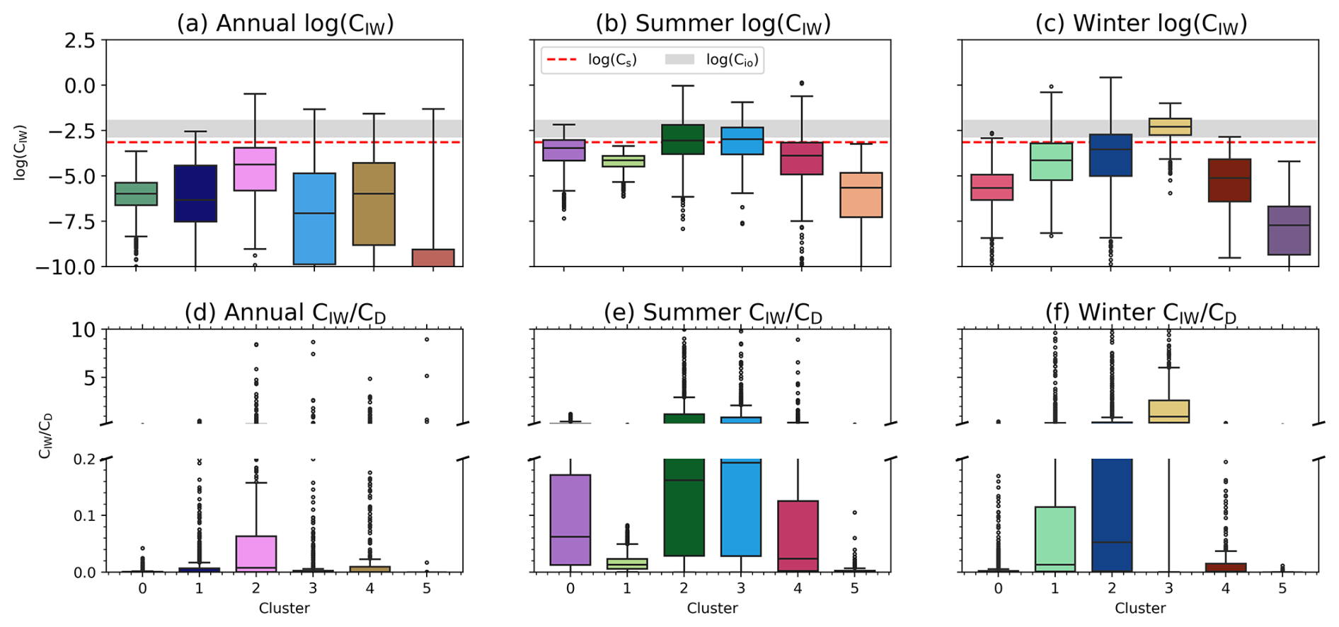
Figure 10 Distribution of internal wave drag C_IW induced by the ice keel calculated from the parameterization expression for each of the clusters based on data averaged: (a, d) annually, (b, e) over the summer months (JJA), and (c, f) over the winter months (DJF). Panels (a)–(c) show the values of C_IW, with grey shaded region representing the range of ice-ocean drag coefficients C_io and skin drag coefficient C_S estimated from observations. Panels (d)–(f) show the ratio between the parameterized values of C_IW for each cluster and the canonical ice-ocean drag coefficient value of $C_{\mathrm{D}}=\mathrm{5.5}\times {\mathrm{10}}^{-\mathrm{3}}$. Note that in (a)–(c), in order to better see the differences across clusters with larger internal wave drag, the y−axis is cropped; so values for some clusters that fall below $\log \left(C_{\mathrm{IW}}\right)=-\mathrm{10}$ and are too small to be shown. Also, note that in (d)–(f), the vertical y-axis is broken into two intervals [0,0.2] and [0.2,10] in order to show the distributions for clusters with both small and large values (e.g., cluster W3).

Now that we have explored the spatio-temporal variability of the nondimensional parameters and the subsequent variability in the predicted values of the IW drag, we put these findings into a broader context in the next section.

6 Discussion

6.1 Implications

In this study, we perform GMM clustering over four nondimensional parameters (lee wave radiation parameter χ, keel criticality J, depth ratio η, and Froude number Fr) to identify parts of the Artic that have similar distirbutions of these parameters. Our clustering is performed both on the annually-averaged data and data averaged over the summer and winter months separately to deduce any seasonal patterns. We find that GMM clustering generally performs well to separate the spatial patterns of perennial multi-year ice (A0–1, S0–1, and W0–1) and of seasonal first-year ice zones (A2–5, S2–5, W2–5) identified based on maps from Serreze and Meier (2019) and Simon et al. (2025). The seasonal clusters also spatially separate the Eurasian (S1, W1) and the Amerasian (S0, W0) basins for both seasons. This agrees with the current understanding of the noticeable differences between the two basins, for example, in terms of the seasonal stratification (Brown et al., 2020). Our estimates of KE dissipation rates from the idealized numerical simulations and the estimates of C_IW from the current parameterization both indicate a differences between the regions of perennial sea ice and seasonal sea ice. This can be important as the proportion of perennial sea ice in the Arctic has been decreasing in the past three decades (Serreze and Meier, 2019).

One of the significant contributions this study is identifying parts of the Arctic that potentially have elevated values of IW drag – but are these values large enough? We can estimate the relative importance of the IW drag by comparing the C_IW values from parameterizations with skin C_s and ice-ocean drag coefficients C_io estimated from observations (Fig. 10a–c). We take the skin drag coefficient value of $C_{\mathrm{s}}=\mathrm{7}\times {\mathrm{10}}^{-\mathrm{4}}$ from the measurements under unridged summer ice by Reifenberg et al. (2025). The range of values for C_io is estimated from various observational studies: 1.3–$\mathrm{12.3}\times {\mathrm{10}}^{-\mathrm{3}}$ (Beaufort Sea, annual cycle by Brenner et al., 2021), 4–$\mathrm{6}\times {\mathrm{10}}^{-\mathrm{3}}$ (Amudsen and Nansen Basins, summer by Fer et al., 2022), 1–$\mathrm{10}\times {\mathrm{10}}^{-\mathrm{3}}$ (Canada Basin, annual cycle by Cole et al., 2017), and 1–$\mathrm{10}\times {\mathrm{10}}^{-\mathrm{3}}$ (average value of $\mathrm{3.4}\times {\mathrm{10}}^{-\mathrm{3}}$, Nansen Basin in July by Randelhoff et al., 2014). However, notably, Kawaguchi et al. (2024) measured that C_io can be as large as 0.13 at times. We also make comparisons to the canonical ice-ocean drag coefficient value of $C_{\mathrm{D}}=\mathrm{5.5}\times {\mathrm{10}}^{-\mathrm{3}}$, which is approximately in the middle the C_io range (Fig. 10d–f). When the IW drag estimates are made with the annually-averaged data, we find that the C_IW values are typically smaller than the measured C_s and C_io values and mostly less than 10 % of C_D. In the regions of perennial sea ice (e.g., S0–1, W0–1), C_IW is still smaller in comparison to the form and skin drag coefficients; we find that at most only 50 % of the points in those clusters have IW drag coefficient values larger than C_D (Fig. 10d–f). However, in some marginal ice zones (e.g., S2–3, W2), C_IW can be 10 %–20 % on average (or even larger for some points) of C_D. The C_IW values for cluster W3 (along Greenland and in the Chukchi Sea) can be as large as or exceeding C_D. Combined, these clusters contain about a third of all data points that we examined over the Arctic for each season (cf. Fig. 5). So, even though the IW drag may be relatively not as important in the pack ice regions in the Central Arctic Ocean, it could be important in the marginal zones, especially in the winter.

It is important to note that the values for the IW drag coefficient C_IW presented here are calculated using the parameterization by McPhee and Kantha (1989). This parameterization was developed for a two-dimensional model assuming small keel height h₀, i.e., small topographic criticality parameter J for a fixed stratification N₀ and relative keel speed u₀. A study by Johnston et al. (2026) recently assessed the parameterizations of form drag for flow over seamounts. They found that the disagreement between numerical simulations and the two-dimensional parameterization also derived for small mount heights (Bell, 1975) increased as J increased. Specifically, they found that the parameterization underestimated the form drag more in comparison to the numerical simulations for larger values of J: at J=1, the parameterized drag was only about one third of the value calculated from the simulations. Their results suggest that the current parameterization for C_IW by McPhee and Kantha (1989) might also be underestimating the drag at larger values of J. In this study, we find many points in across the Arctic with J≳1: 67 % of all grid points in the annual average, 91 % during the summer months, and 7 % during the winter months. Our findings indicate that this supercritical regime J≳1 might be an important parameter regime, especially during the summer, but it is not well-represented by the current parameterization and needs to be re-evaluated through future numerical studies.

Another assumption made in the McPhee and Kantha (1989) model of ice keel-flow interaction is that the pycnocline lies below the ice keel, meaning that the depth ratio η is greater than unity. However, in the summer, the canonical mixed layer can be absent in parts of the Arctic, such that even the near-surface ocean layers are stratified (Randelhoff et al., 2017). We also find that approximate 67 % of data points in the summer months (and 1.9 % for the annual and 8.4 % for the winter data) have the depth ratio η<1. For the idealized numerical simulations conducted to assess the parameterization of C_IW, the absence of the mixed layer does not pose a problem, as it would be just the limiting case of setting the nondimensional parameter η to zero (as the mixed layer depth z₀=0). In on our preliminary numerical simulations (clusters S0, S2, W2) with the mixed layer depth less than or about the keel depth (η≲1), we find kinetic energy and dissipation rates to be larger by at least an order of magnitude in comparison to the other parameter value combinations examined in the numerical simulations here (Table 2). In particular, in cases with η<1 considered here (S0 and S2), we find an energetic flow field with many small-scale motions that are possibly enhancing the energy cascade and dissipation (Fig. 11a–c, e–g). Overall, we would expect that smaller η would enhance the IW generation and the IW drag as the ice keel would be in a more direct contact with the stratified layer, potentially without the buffer of the mixed layer. Therefore, the parameter regime of such smaller η values might not be well-captured in the current IW drag parameterization and needs to be further explored through numerical simulations.

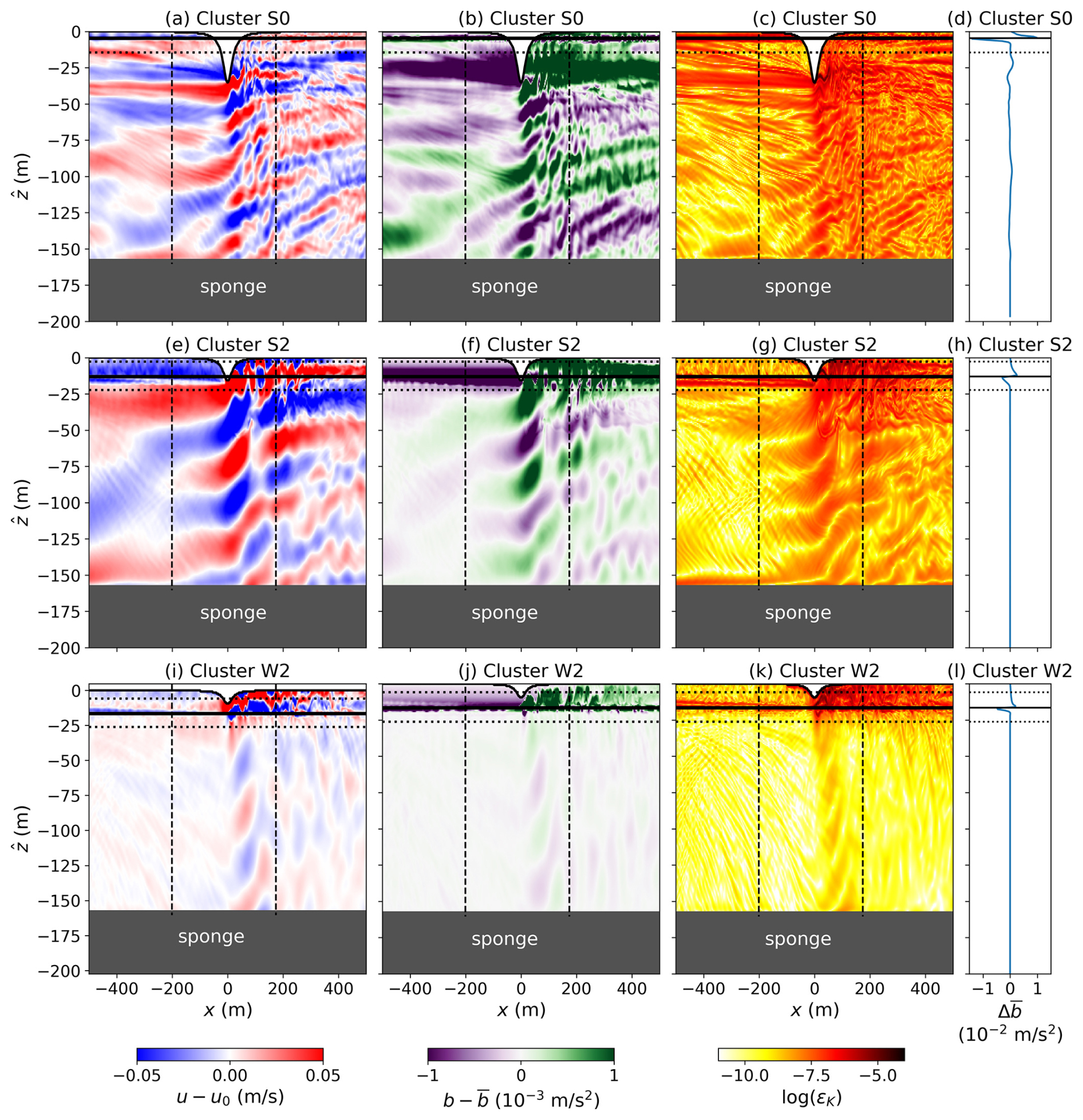
Figure 11 Snapshots from numerical simulations set with nondimensional parameters for GMM clusters S0 (a–d), S2 (e–h), and W2 (i–l): (a, e) turbulent horizontal velocity u−u₀, (b, f) buoyancy perturbations, i.e., deviations from horizontally-averaged $\stackrel{\mathrm{‾}}{b}\left(z\right)$, (c, g) log of kinetic energy dissipation ϵ_K, and (d, h) buoyancy deviation from initial conditions $\mathrm{\Delta }\stackrel{\mathrm{‾}}{b}=\stackrel{\mathrm{‾}}{b}\left(z\right)-b_{\mathrm{0}}\left(z\right)$. The thick black horizontal black lines in each subplot indicate the pycnocline $\widehat{z}=z_{\mathrm{0}}$ and horizontal dotted lines delineate $\widehat{z}=z_{\mathrm{0}}\pm \mathrm{10}$ m. In (a)–(c), (e)–(g), dashed vertical lines delineate the region $x\in [-\mathrm{200},\mathrm{200}]$ m, which is used for horizontal averages and integrals. All snapshots are for the last timestep (after 6 h) of simulation time.

With recent GPU-acceleration of computational fluid dynamics numerical codes (e.g., Oceananigans.jl), Johnston et al. (2026) conducted a large numerical simulation sweep to test the existing parameterizations for the drag due to steady and tidal flows interacting with topographic obstacles along the ocean floor (i.e., seamounts). However, that problem has a different set of nondimensional parameters compared to the sea ice-flow interaction problem. Namely, additional nondimensional parameters to characterize the ratio between mixed layer depth and keel depth (η) and the ratio of the kinetic energy of the flow relative to the potential energy due to the buoyancy jump across the pycnocline (Fr) are relevant in the upper Arctic Ocean stratification, whereas constant stratification is assumed near the ocean bottom. Therefore, there is a need for similar studies with a consistent numerical set-up to test the existing sea ice drag parameterizations. Previous modeling efforts typically have only considered the variability of one or two of the relevant nondimensional parameters and only certain parameter regimes, e.g., only relatively deep ice keels (η=0.25–2 in Zhang et al. (2022) and De Abreu et al. (2024)) or in contrast, homogeneous fluid (η→∞ in Zu et al. (2021) and Wang et al. (2025)). We find η to be in the range of [0,140] and concentrated in the $\mathit{\eta }\in [\mathrm{2},\mathrm{4}]$ range in the annually-averaged and winter-averaged data and in the $\mathit{\eta }\in [\mathrm{0},\mathrm{1.5}]$ range for the summer-averaged data. From our preliminary numerical simulations, we also find that the kinetic energy metrics might be enhanced for mid-range values of η∼5 depending the values of other nondimensional parameters. In the absence of well-distributed observational data of Arctic ice keel and near-surface ocean flow characteristics, our results provide a good starting point to consider for parameter sweeps in future numerical studies. Our results also suggest that certain joint ranges of parameter values might not need to be investigated in detail (e.g., large χ and large J combinations).

We can also compare the kinetic energy metrics from our numerical simulations with observations. Many observational studies estimate internal wave dissipation rates in the Arctic to be within the 10⁻¹⁰–10⁻⁹ m² s⁻³ range (Scheifele et al., 2018; Kawaguchi et al., 2019; Fine and Cole, 2022; Fer et al., 2022). These values are smaller than observational measurements of up to 10⁻⁸ m² s⁻³ in the upper parts in other global ocean regions (Waterhouse et al., 2014). In our idealized numerical simulations, we find the dissipation rates below the pycnocline to be generally on the order of 10⁻⁹ m² s⁻³, which is within the range of observed values (Fig. 12b). However, larger values of ϵ have been found close to the sea ice, in particular when the mixed layer is thin (Fer et al., 2022; Reifenberg et al., 2025). We also find larger values of kinetic energy dissipation within the pycnocline region and above the pycnocline in the case of numerical simulations with smaller η (shallower pycnocline) (e.g., simulations A0, S0, S2, and W2 in Fig. 12d, e). These results suggest that depending on the sea ice and flow characteristics, there could be a spatio-temporal variability in the dissipation and subsequently diapycnal mixing rates in the Arctic. Note that our estimates of the dissipation rates from the numerical simulations include energy loss from all motions that are deviations from the background flow (predominantly the generated IWs) and the model viscosity is larger than the molecular viscosity of sea water. Although some previous studies have made comparison of flow energetics and in particular dissipation rates with observations (e.g., Nikurashin and Ferrari, 2010a; De Abreu and Timmermans, 2026), any direct comparisons with observational values should be cautious.

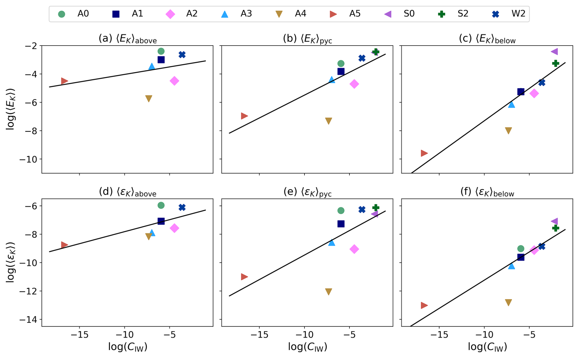
Figure 12 KE metrics (a–c) KE E_K and (d–f) KE dissipation ϵ_K calculated from numerical simulations plotted against IW drag C_IW estimated from the McPhee and Kantha (1989) parameterization. KE metrics are area-averaged over different regions of the simulation domain: (a, d) above the pycnocline above, (b, e) within the pycnocline pyc, and (c, f) below the pycnoline below) as defined in Eqs. (20)–(22). Each scatter symbol corresponds to a different simulation as denoted in the legend (annual clusters A0–5, summer clusters S0 and S2, and winter cluster W2). Nondimensional parameters for these simulations are shown in Table 1 and raw values of 〈E_K〉 and 〈ϵ_K〉 can be found in Table 2.

Using our numerical simulation results, we evaluate how well the C_IW parameterization captures the variability in KE metrics. In the region below the pycnocline (Fig. 12c, f), parameterized C_IW values generally capture the trend in the orders of magnitudes of both E_K and ϵ_K well, though it might overestimate the KE and dissipation rates for large Fr (weak pycnocline, A4) and underestimate them for small η (shallow mixed layer, S0). Parameterized C_IW values are not as well correlated with E_K and ϵ_K above the pycnocline (Fig. 12a, d) and around the pycnocline (Fig. 12b, e), which might be expected as the parameterization was primarily developed for IW energy flux below the pycnocline into the stratified interior. Of course, there are many real-ocean processes that are missing in our idealized numerical simulations as will be discussed in Sect. 6.2, and in this study we only analyze nine specific cases. Therefore, we caution against overinterpreting the numerical values and trends of ϵ_K in our numerical simulations without a more thorough parameter sweep.

Finally, when discussing the role of ice keels in the Arctic, it is important to consider climatological changes and shifts in sea ice dynamical regimes. One potential change is sea ice smoothing. Measured from aircraft, above-sea surface ice ridges have significantly decreased in height and ridge density over the last 30 years. This loss is especially prominent in parts of the Arctic that are experiencing loss of multi-year ice like the Beaufort Sea and the Last Ice Area (Krumpen et al., 2025). Smoother ice leads to reduction of atmospheric surface drag coefficient on ice ridges. While this is not direct evidence for changes in the under-sea surface keel height and density, it is plausible that there is some correlation between the above- and under-sea surface ice properties. This implies that understanding the effects of ice keels on ocean mixing is important, as these effects could be reduced if the ice ridges become smoother. A large portion of these areas that Krumpen et al. (2025) found to have sea ice ridge smoothing are within Cluster A0 (and seasonally S0 and W0) in our dataset. This cluster is characterized by relatively large J and small η that enhance kinetic energy dissipation. Therefore, smoothing of the ice keels (a reduction in h₀, so a reduction in J and η) can substantially change the ice-ocean dynamics in this region.

Arctic stratification has also changed in the last several decades. For example, through analysis of water column observations, Polyakov et al. (2018) found changes in both the pycnocline depth, approximated as the mixed-layer depth z₀ in this study, and the change in buoyancy across the pycnocline (Δb in this study). Specifically, they found a pan-Arctic increase in z₀, possibly due to surface-layer freshening or deepening of the mixed-layer due to intensification of wind-driven mixing (Polyakov et al., 2020). Combined with potentially smaller h₀ from sea-ice smoothing, this would result in an increase in η and less ice keel-induced turbulent dissipation and mixing and reduced IW drag in the upper ocean. Polyakov et al. (2018) also found an increase in Δb in the Amerasian Basin (Cluster A0 and seasonally S0 and W0), which would correspond to a decrease in Fr. Based on our numerical simulations, this decrease in Fr would reduce KE and dissipation rates. However, the relationship between the IW drag and Fr, at least in the current parameterization, is nonlinear (Fig. 9(right)), so further analysis is needed to assess the ocean's response to these changes.

6.2 Limitations

One of the main limitations of this study is that we use data from another model (Flocco et al., 2024) to estimate the distribution of dimensional and nondimensional parameters across the Arctic. While this is unavoidable as there are still no comprehensive pan-Arctic datasets for all the variables that we would need, we need to discuss how the differences in the values of the underlying dimensional parameters between the model output and the real ocean can affect our findings. For example, Flocco et al. (2024) showed that their model in general overestimates the sea ice drift speed over most of the Arctic and across seasons in comparison to the observational data from the National Snow and Ice Data Center Polar Pathfinder dataset. This is consistent with climate models typically overestimating sea ice drift (Wang et al., 2023). From Flocco et al. (2024), the overestimation of the sea ice drift by the model is largest during the winter in the marginal sea ice areas. These regions are part of our clusters W2 and W3 (Fig. 5i, l) that have relatively large C_IW predicted by the parameterization (Fig. 10c, f). For cluster W3, this is in part because of the larger Froude number Fr (Fig. 6f) that is proportional to the relative sea ice speed u₀. Therefore, an overestimate of the ice drift by the model could, in turn, overestimate the IW drag C_IW.

In Sect. 6.1, we noted the relative importance of the regime with smaller depth ratio η values. However, as noted in Flocco et al. (2024), the pycnocline or mixed layer depths shallower than 10 m cannot be accurately quantified in the NEMO model, hence, they are not present in our clustering results. This means that in addition to the ranges of values of η presented in this study, smaller values of η→0 would have to be considered when conducting numerical simulations to evaluate the parameterization of the IW drag. Accurate values of ice keel depths h₀ are also necessary for estimating the depth ratio η, so we also compare the distribution of ice keel depths h₀ with observed values. Figure S2 shows the distribution of h₀ from the entire Flocco et al. (2024) model output (not just our filtered data within the lee wave radiation regime) with the distribution from a large keel dataset by Metzger et al. (2021). The distributions are in overall good agreement, especially if we consider h₀<9 m as one bin, as data for h₀<6 m was not presented in Metzger et al. (2021). Notably, other observational studies (e.g., Cole et al., 2017; Brenner et al., 2021) have found such smaller keel depths (h₀<6 m). These comparisons suggest that the distribution of the h₀ values used in this study is in a reasonable agreement with the observations.

Other limitations of the study stem from the choices made in our numerical simulations that resulted in us not considering certain physical processes. One such limitation in the numerical set-up of this study is that we neglect the skin and form drag (i.e., the turbulent ice-ocean boundary layer) by imposing free-slip boundary conditions along the ice keel boundary. While we chose to implement this approach in order to separate the effects of IWs and because our results would change due to our subjective choices of the drag coefficients, in the real Arctic Ocean, all three of the drag components would have an effect on the ice keel speeds. Because the shape of the keel in our simulations and the conceptual model is not allowed to change, we neglect the effect of turbulent heat fluxes that can melt the sea ice. This process can be complicated. For example, Skyllingstad et al. (2003) found that while ice keels enhance turbulence, their effects on melting can depend on blocking of the flow and trapping of fresh water. This can alter the shape of the ice keel, though we do not expect it to take effect on the short timescales of our simulations. The choice of shape to represent the ice keel also plays an important role. A recent study examining submarine sonar data (Eilers and Bradley, 2026) found that keels can have different shapes, e.g., triangular shapes, cusp shapes like Versoria used in this study, and trapezoidal shapes that have a flatter bottom. Their study also found that the keel shape is dependent upon the keel depth and processes that the keel undergoes throughout its lifecycle, e.g., it may form in a pointier shape but flatten along the bottom due to accelerated bottom melt in the summer. Such differences in keel shapes can affect IW generation and drag.

In this study, we also assume that the wind has already transferred momentum to the ice keel to move it, and hence neglect modelling the atmosphere-ice stress. This is a common assumption for an idealized process study (e.g., Zu et al., 2021; De Abreu et al., 2024; Wang et al., 2026) such as the current one aimed to isolate the dynamics of internal wave generation by the ice keels, However, in the ocean, momentum transfer within the atmosphere-ocean-ice coupled system can be simultaneous and is a more complicated process (Brenner et al., 2021). Another nondimensional parameter, the Nansen number, which measures the ratio between the atmosphere-ice and ice-ocean drag coefficients scaled by the ratio of air and sea water densities, can be useful to characterize this coupling. Better-constrained Nansen number, possibly through further observational campaigns of measuring atmosphere-ice and ice-ocean drag coefficients (e.g., Brenner et al., 2021; Fer et al., 2022; Kawaguchi et al., 2024; Reifenberg et al., 2025), would be important for more accurately capturing the three-way coupling in climate models.

The two-dimensional set-up of this model also neglects certain physical mechanisms, e.g., three-dimensional turbulence and three-dimensional effects due to flow splitting around the keel (Nikurashin et al., 2014). Because we only model a single keel, we neglect ice keel sheltering effects from upstream keels, which have been found to affect the dynamics of the flow and skin drag parameterizations in previous modelling studies (Wang et al., 2025). The parameterization in McPhee and Kantha (1989) also omits the effects of rotation, so we also consider motions on time scales shorter than the inertial period in our numerical simulations. The effect of rotation is two-fold. First, it can shrink the range of lee wave radiation from $\mathrm{0}<\mathit{\chi }<\mathrm{1}$ (non-rotating case) to ${\displaystyle \frac{f}{N_{\mathrm{0}}}}<\mathit{\chi }<\mathrm{1}$ (rotating case). However, in our dataset we find that less than 0.2 % of points have $\mathit{\chi }<{\displaystyle \frac{f}{N_{\mathrm{0}}}}$, so perhaps this is not a substantial limitation. However, in the presence of rotation, near-inertial waves are generated on the timescales of $\mathrm{2}\mathit{\pi }/f$ (order of 11–17 h). Near-inertial waves that can interact with lee waves to enhance dissipation (Nikurashin and Ferrari, 2010b; Zemskova and Grisouard, 2021), which is not considered here or in the McPhee and Kantha (1989) parameterization. This effect of the rotation via the near-inertial wave generation can be examined further in subsequent numerical studies running the simulations for longer periods of time.

Finally, in this study, we made a particular choice of six GMM clusters based on the statistical information from the BIC score and by considering the interpretability of our results. For the purpose of the discussion here, we focus on the summer-averaged data, though similar conclusions can be made for winter clusters. Based the BIC curve (Fig. 3), we should have chosen a larger number of clusters (K≈10 clusters) in order to improve the GMM's ability to capture the variability in the data. Having more clusters would have allowed us have better-constrained clusters, i.e., reduce the standard deviation of the nondimensional variable ranges within each cluster and the overlap between clusters (Figs. 6, 9). However, this would have been too many clusters to interpret in terms of physical regimes. On the opposite end of the spectrum, we can also divide the Arctic broadly into three regimes similarly to our discussion of the results in Sect. 5.1: (1) the central Arctic with perennial ice, (2) marginal ice regions with larger η (smaller keel depth, deeper pycnocline) and without substantial IW generation, and (3) marginal ice regions with intermediate η that support IW generation. However, such broad characterization would return a wide range of nondimensional parameter values for the central Arctic, which is perhaps not an insightful result. In order to examine the tradeoff between the accuracy of representing the statistical distribution of the nondimensional parameters (i.e., large K) and ease of interpretation (i.e., small K), we show the spatial distribution of GMM clusters for K=4, 5, and 7 in Fig. S3 for comparison with K=6 in Fig. 4b. Too few clusters (e.g., K=4–5) leaves the entire central Arctic region as a single cluster. However, for K=7, the GMM algorithm returns a relatively consistently clustered centered Arctic, separating the Amerasian and Eurasian basins, and the outer eastern Eurasian seas. Increasing the number of clusters K in this range (6–7) seems to predominantly break marginal regions into even smaller clusters. Based on this analysis, we choose K=6 to strike an overall balance, though recognizing that this choice is somewhat subjective.

7 Conclusions

In our study, we combined upper ocean stratification parameters and keel characteristics, such as depth, spacing, and relative speed from the sea ice-ocean coupled NEMO–CICE model output (Flocco et al., 2024) into four nondimensional parameters to identify ranges of values and parameter regimes of ice keel-ocean interactions. Specifically, we examined these parameters within the theoretical framework of McPhee and Kantha (1989) with a steadily moving ice keel along the surface of a two-layer upper ocean, such that an upper mixed layer is separated from the weakly stratified lower layer by a sharp pycnocline. These nondimensional parameters captured (1) lee wave propagation potential in the stratified layer (χ), (2) nonlinearity of the waves (J), (3) mixed layer depth relative to the keel depth (η), and (4) the strength of the pycnocline relative to the flow shear (Fr).

Applying the GMM unsupervised clustering algorithm to these four nondimensional parameters allowed us to uncover statistically coherent clusters that potentially correspond to distinct dynamic environments. The GMM fit used only nondimensional parameter values at each grid point (no geographic predictors), so the geographic coherence in our results reflects underlying mechanics rather than explicit location features. Constructing the clusters using seasonally-averaged data revealed temporal differences in the nondimensional parameter regimes and highlighted the differences between the Amerasian and Eurasian basins. Both based on the IW drag values predicted by the McPhee and Kantha (1989) parameterization and from our estimates of fluctuating KE dissipation rates, we found that near-land boundary regions with only seasonal sea ice cover were likely to have less impact of the moving ice keels on the ocean flow and internal wave generation due to relatively not steep ice keel sides and relatively shallow keel depths compared to the mixed layer depth. In the parts of the Central Arctic Ocean characterized by perennial sea ice we found larger kinetic energy magnitude, dissipation rates, and IW drag values due to steeper and deeper ice keels (larger values of J and smaller η).

The results of this study also revealed the ranges of values for these four nondimensional parameters across the Arctic, which can be used in future numerical studies of the interactions between the sea ice and the upper ocean. A prototype for such simulations is presented in this study. Numerical simulations are a powerful tool to study a particular phenomenon and perform controlled parameter sweeps. However, in order to groundtruth the parameterizations derived from numerical simulations, observational measurements are necessary. In particular, we would need simultaneous measurements for the values of the input dimensional variables (u₀, k₀, h₀, z₀, Δb, N₀) and the values that we would like to parameterize, e.g., IW drag and KE dissipation. As we find significant spatial and seasonal variability, especially differences between perennial and seasonal ice, long-term observational measurements in different parts of the Arctic would be helpful to validate the parameterizations.