Parameterization of the snow fracture energy to model the onset of crack propagation in snowpack models

Snowpack models are widely used to complement field observations in avalanche risk forecasting. They help estimate key indicators related to dry-snow slab avalanche triggering processes, such as failure initiation and crack propagation. In recent decades, several frameworks have been developed to model the onset of crack propagation, typically characterized by the critical cut length (the cut length beyond which an initial crack starts propagating), measurable in the field using the Propagation Saw Test (PST). However, these models often depend on poorly constrained parameters, particularly, the weak layer fracture energy w_f. In this work, we relate the fracture energy to snow properties that can be measured directly or simulated by detailed snowpack models. To this end, we compute the min-cut on about 300 three-dimensional snow microstructure images. The min-cut represents the smallest ice interface that would need to be fractured to separate two opposing sides of the structure, and can therefore be interpreted as a proxy of fracture energy. We fitted a relation between the min-cut and snow properties that can be measured or simulated, namely density and grain morphology. The min-cut is then linearly related to the fracture energy w_f using measurements from Richter et al. (2019), which track weak layers across multiple seasons and sites using PST and observed profiles. We retrieved w_f by inverting the WEAC slab model (Weißgraeber and Rosendahl, 2023): we supply the model with slab characteristics that are either obtained from field measurements or from Crocus snowpack simulations and solve w_f for the given PST-derived cut lengths. This yields a relationship between w_f and the min-cut, calibrated for the grain types most commonly associated with dry-snow slab avalanche release (faceted crystals and depth hoar) under predominantly Mode I loading conditions. After calibration, w_f is evaluated in two slab models of different complexity for their ability to reproduce measured critical cut lengths, using both observed data and Crocus outputs. Although the correlation between min-cut and w_f remains moderate (i.e. R of 0.5 at most), likely due to measurement and modeling uncertainties, the parameterization demonstrates an added-value over the use of a constant w_f in reproducing realistic critical cut lengths. Moreover, the proposed parameterization performs well for identifying and monitoring weak layers over the course of the season. Its consistent performance across slab models and strong results using Crocus outputs highlight its potential for operational dry-snow slab avalanche hazard monitoring.

1 Introduction

Snow avalanches threaten lives and infrastructures in snow-covered mountainous regions (e.g. Techel et al., 2016; Ortner et al., 2025). Accurate avalanche forecasting enables authorities to implement short-term mitigation strategies, such as road closures, evacuations, or deployment of emergency services (e.g. Leone et al., 2014). Forecasting is also important for snow professionnals and backcountry recreationists to choose safer routes and avoid hazardous zones (EAWS, 2026). Observations of snow stratigraphy and stability tests provide valuable information for now-casting avalanche danger. However, these observations are sparse both spatially and temporally due to the time and human resources required for their collection and do not provide any forecast for the next hours and days. To complement these direct measurements, detailed snow models such as Crocus (Vionnet et al., 2012; Lafaysse et al., 2025) and SNOWPACK (Wever et al., 2015) are widely used (Morin et al., 2020). These models simulate the evolution of individual snow layers and their properties, allowing for continuous monitoring of snowpack changes beyond what observations alone can capture. By being forced with numerical weather models, they can forecast future snowpack states, offering spatially and temporally comprehensive predictions essential for avalanche risk assessment.

Assessing the avalanche danger from several simulated snow profiles is not straightforward (Morin et al., 2020). Among loose and slab avalanches, slabs avalanches are generally the most dangerous because they mobilize larger snow volumes (McClung and Schaerer, 2006). But they are also the most challenging to predict as their release results from a series of complex mechanisms (Reuter and Schweizer, 2018; Schweizer et al., 2021): failure initiation in a weak layer below a slab, onset of crack propagation, dynamic crack propagation, opening of the tensile crown crack in the slab, and its sliding down the slope. To deliver avalanche-oriented information from snowpack simulations, it is necessary to develop indicators of the likelihood of these mechanisms to occur for a given snow profile. Among these mechanisms, the onset of crack propagation in the weak layer has been a central topic in avalanche research since the 2000's with the pioneering work of McClung (1979), van Herwijnen and Jamieson (2005), Gauthier and Jamieson (2008). At the onset of crack propagation, an initiated crack in the weak layer reaches a critical size and begins to self-propagate independently of what initiated it. This critical point can be described by the critical cut length a_c (m) in a conceptual propagation saw test (PST) (van Herwijnen and Jamieson, 2005; Gauthier and Jamieson, 2006, 2008). In practice, the critical cut length is system-specific and varies significantly depending on a wide range of factors, including the characteristics of the slab and the weak layer, as well as the geometric configuration of the snowpack (unbound at the sides or embedded, slope angle).

Modeling of the critical cut length typically relies on linear fracture mechanics and the Griffith criterion (Griffith, 1920; Margolin, 1984), through an energy balance performed over the deforming slab weak-layer system, also accounting for the substratum depending on model complexity. At the onset of crack propagation, the energy release rate related to elastic deformation and gravity potential energy equals the energy to extend the crack surface area in the weak layer (Heierli et al., 2008). The critical cut length a_c thus depends on both how the slab deforms when it loses support from the weak layer, and the specific fracture energy of the weak layer w_f (J m⁻²) (Sigrist and Schweizer, 2007). On one hand, the energy released by the slab during crack propagation can be modeled using beam theory – the slab thickness is generally small compared to the other dimension of the slab or PST snow column – (Heierli et al., 2008; Weißgraeber and Rosendahl, 2023), or simulated using finite elements (Schweizer et al., 2011; Van Herwijnen et al., 2016; Reuter and Schweizer, 2018). In all approaches, the slab energy release is primarily controlled by the slab weight and its effective elastic modulus. Differences between modeling frameworks mainly arise from assumptions regarding boundary conditions (e.g., embedded versus free slab ends in PST configurations), the extent of the simulation domain (e.g., whether deformation energy of the weak layer and the underlying substratum is included), the treatment of potential slab touch-down, and the representation of slab stratigraphy and layering.

In contrast, the fracture energy of the weak layer is rarely determined independently. Instead, it is most often inferred a posteriori by inverting the critical cut length measured in PST experiments, using a slab mechanical model fed by the measured or simulated slab stratigraphy (Schweizer et al., 2011; Van Herwijnen et al., 2016; Schweizer et al., 2016; Adam et al., 2024). An exception is the approach introduced and developed by Reuter et al. (2013, 2015), Reuter and Schweizer (2018), Reuter et al. (2019) in which the weak-layer fracture energy w_f is approximated as the minimum penetration resistance integrated over a given length, derived from snow micropenetrometer (SMP) measurements, then used to predict the critical cut length a_c.

To our knowledge, only Gaume et al. (2017) and Richter et al. (2019) have attempted to parameterize a_c as a function of snowpack model variables. Their approach relies on an empirical stress-strength formulation derived from DEM simulations of a PST configuration, in which the slab is discretized as a sphere assembly and the weak layer as a collapsible triangular arrangement of bonded spheres (representative of depth/surface hoar). Richter et al. (2019) improved the parameterization by addressing the mismatch between the collapse height of the initial parameterization and the SNOWPACK stratigraphy resolution via an empirical fit accounting for grain size and density. While lacking a fully established physical basis, this approach provides a practical model implementation, though it currently requires human expertise to pre-identify weak layers.

In summary, forecasting slab avalanche formation requires, among other processes, characterizing the propensity of cracks to start to propagate spontaneously within snow layers, which is partly governed by the weak-layer fracture energy w_f. Recent literature mentioned that common predictors for fracture toughness, related to fracture energy through Irwin's relation, in highly porous materials include density and microstructure (Adam et al., 2024). Yet a generic parameterization of w_f as a function of simulated snow layer variables is currently lacking. In this paper, we link w_f to density and grain morphology descriptors that can be simulated by detailed snow models. To do so, we first relate density and grain morphology to the min-cut surface area on 3D images of the snow microstructure. The minimum surface area quantifies the smallest ice interface that would need to be fractured to separate two opposing sides of the microstructure (Hagenmuller et al., 2014). As suggested by LeBaron and Miller (2014), this minimum represents a lower bound for the fracture energy and thus serves as a physical proxy for w_f. Eventually, we scale the simulated min-cut surface area to pseudo-observations of w_f obtained using the state-of-the-art slab models (Weißgraeber and Rosendahl, 2023; Rosendahl and Weissgraeber, 2024) and PST data collected by Richter et al. (2019). All in all, we obtain a relation between density, grain morphology, and weak layer fracture energy. We show that this parameterization helps predict the critical cut length measured by PSTs.

2 Materials and Methods

2.1 Slab models

The critical cut length beyond which a crack starts to propagate depends on the mechanical behavior of the weak layer and the overlying slab and on the geometric configuration of the snowpack considered. Therefore, in order to estimate the fracture energy w_f from a PST or to even predict the critical cut length of a given snowpack stratigraphy, it is necessary to model the deformation of the slab. Specifically, such a model is required to quantify the potential energy (gravity and elastic) released by the slab as it loses basal support from the weak layer during crack propagation. In this work, we used two slab models: the WEAC numerical model by Weißgraeber and Rosendahl (2023), Rosendahl and Weissgraeber (2024) and the polynomial model by Heierli et al. (2008). The WEAC model represents the current state-of-the-art and has been used to invert PST results into pseudo-measurements of w_f. Both models are then used to quantify a_c from simulated weak layer fracture energy and slab stratigraphy. In this case, the analytical model by Heierli et al. (2008), despite its simplicity, is particularly valuable due to its computational efficiency, making it well-suited for integration into large-scale simulations such as land surface models.

2.1.1 WEAC model

We employed the python implementation (WEAC package; Rosendahl and Weissgraeber, 2024) of the model described in Weißgraeber and Rosendahl (2023). This model considers the deformation of a multi-layered elastic snow-slab resting on an idealized elastic foundation (Fig. 1b). The slab can consist of multiple layers with distinct thicknesses, densities and elastic modulus, and the model accounts for bending-extension coupling within the slab. Conditions within the slab and weak layer are chosen to account for the mixed-mode stress conditions (mode I and II). WEAC provides an analytical solution for computing slab displacements, weak layer stress distributions, and energy-release rates. In this study, we used the version 3.1.4 of the WEAC package (Rosendahl and Weissgraeber, 2024). The application of the model in this study is done considering a PST cut upslope (if incline different from 0°) with the touchdown feature enabled (but never triggered in our application) (Fig. 1b). The height of the weak layer is set at 3 cm (default value). The elastic modulus E (Pa) of the weak layer and the slab are parameterized as a function of layer density ρ (either modeled or measured) using Gerling et al. (2017) formulation slightly modified by Bergfeld et al. (2023):

$$\begin{array}{}\text{(1)}& E=\mathrm{6.5}\times {\mathrm{10}}^{\mathrm{9}}\mathrm{Pa}{\left({\displaystyle \frac{\mathit{\rho }}{{\mathit{\rho }}_{\mathrm{ice}}}}\right)}^{\mathrm{4.4}}\end{array}$$

with ρ_ice = 917 kg m⁻³ the ice density.

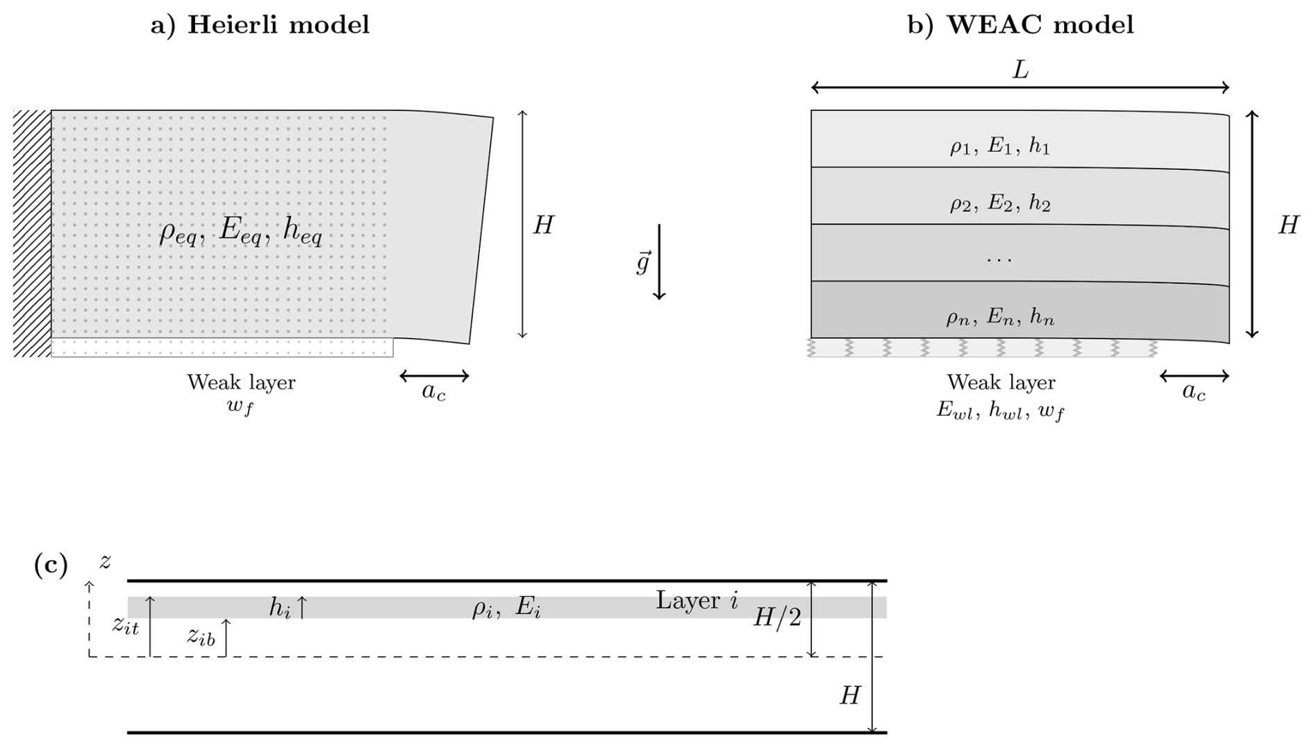
Figure 1 Schematic representation of (a) the Heierli model, (b) the WEAC model and (c) the description of the slab with the variables and reference framework used to calculate the equivalent modulus of elasticity E_eq. Please note that in panel (a), the dotted area is considered to be non-deformable.

The impact of these assumptions, namely the fixed weak-layer thickness and the elastic modulus parameterization of Bergfeld et al. (2023) on the w_f values retrieved by inversion (see Sect. 3.2.2) is assessed and discussed in the sensitivity analysis presented in Appendix B.

2.1.2 Heierli model

The so-called anticrack model was initially developed by Heierli et al. (2008). We used the version described in details by Schweizer et al. (2011). In this model, a homogeneous equivalent slab is represented by a Timoshenko beam fixed on its left side, deforming under its weight and partial absence of basal support (Fig. 1a). The weak layer is assumed to be infinitely stiff and only the elastic strain energy of the overhanging part of the block (above the saw cut) is considered. The model relates the weak layer fracture energy w_f, to the critical cut length a_c and the equivalent slab characteristics: height H, elastic modulus E and density ρ. The slab height H is the sum of the slab layer thicknesses h_i. The slab density is the average slab density ρ = $\frac{\sum {\mathit{\rho }}_i{h}_i}{\sum h_i}$. For equivalent elastic modulus of a multi-layered slab, we rely on the same laminate plate theory as in Weißgraeber and Rosendahl (2023). Specifically, we apply Eqs. (8c) and (9b) of Weißgraeber and Rosendahl (2023), derived for mode I deformation:

$$\begin{array}{}\text{(2)}& E=\mathrm{4}{\displaystyle \frac{{\sum }_i{E}_i\left(z_{i\mathrm{t}}^{\mathrm{3}}-z_{i\mathrm{b}}^{\mathrm{3}}\right)}{H^{\mathrm{3}}}}\end{array}$$

with E_i the young modulus of the layer i, and z_it and z_ib, respectively, the top and bottom of each layer i as illustrated in Fig. 1c. Again, the layer elastic modulus is determined using the density parameterization of Gerling (Eq. 1). It is important to note that this formulation of the equivalent modulus for a multi-layered slab differs from the simpler formulations proposed by Heierli et al. (2008), Schweizer et al. (2011). However, apart from the most complex computation of the equivalent slab modulus, the rest of our implementation directly follows the works of Heierli et al. (2008), Schweizer et al. (2011).

2.2 Snow model: SURFEX-Crocus

SURFEX-Crocus (Vionnet et al., 2012; Masson et al., 2013; Lafaysse et al., 2025) is a coupled system including a land surface model, SURFEX-ISBA (Noilhan and Mahfouf, 1996) with the Crocus snow model (Brun et al., 1992; Vionnet et al., 2012). Crocus belongs to the most detailed class of snow models, including SNOWPACK (Wever et al., 2015). It explicitly models the snowpack stratigraphy and describes the snow microstructure by its density, sphericity and specific surface area. This model was initially developed for local, single-point, simulations to support the operational forecasting of avalanche hazard by Météo-France. Indeed, its description of the stratigraphy and its layering management enables to follow the evolution of the properties of each layer and, for example, derived indicators of mechanical stability to estimate avalanche hazard (Giraud et al., 2002). In this study, we used the version 9.0 of SURFEX-Crocus (Lafaysse et al., 2025).

2.3 Data

2.3.1 Microstructure 3D images and min-cut

Three-dimensional images of snow microstructure were used to compute the minimum cut surface area (min-cut) of various snow samples and to relate it to the snow density and morphology descriptors. We used tomographic data previously measured with X-ray tomography and already binary-segmented. They were gathered from previous studies: Calonne et al. (2011), Hagenmuller et al. (2016, 2019), Peinke et al. (2020), Hagenmuller and Carmagnola (2020), Fourteau et al. (2022), Bernard et al. (2023), Dick et al. (2026). To speed up the computations, the initial cubic images were downscaled by a factor of two, resulting in a voxel size of about 20 µm. The image side length varies between 5 and 12 mm. Each snow image was initially labeled with a snow type according to the international classification (Fierz et al., 2009). In total, 271 snow images were considered.

The min-cut surface area quantifies the smallest ice interface that must be fractured to separate two opposing sides of the microstructure. We used the algorithm of Hagenmuller et al. (2014) with a 26-connectivity to calculate the min-cut surface area in the three Cartesian directions. We normalized the min-cut values by the sample cross-section and retained only the minimal value in the three directions as a fracture energy proxy. For the sake of simplicity, we call, hereafter, this minimal value with no units the min-cut and denote it ζ. In addition, the ice fraction ϕ was derived from the 3D images by voxel counting.

2.3.2 Propagation saw tests and observed snow profiles

Two datasets containing propagation saw test measurements and observed snow profiles are used in this study. Both are derived from field campaigns described in detail in Richter et al. (2019). They cover two high elevation sites above Davos, Switzerland: the Weissfluhjoch site (WFJ2; 46.830° N, 9.809° E) located at 2536 m and the Wannengrat site (WAN7; 46.808° N, 9.788° E) located at 2442 m, approximately 3 km apart from the WFJ2 site.

Data were collected over three winter seasons, from 2014–2015 to 2016–2017 at site WAN7, and two seasons, from 2015–2016 to 2016–2017 at site WFJ2. During these seasons, a total of seven layers were tested at least once, most of them on a weekly basis for around two months, and for some, several PSTs were carried out on the same date, allowing variability or measurement uncertainties to be taken into account. All of the weak layers were tested at site WAN7, and three of them at both sites. In what follows, they will be referred to using the abbreviation of their grain type according to Fierz et al. (2009) followed by their burial date in year-month-day format (i.e. YYMMDD): FC141216 (WAN7), SH150124 (WAN7), DH151201 (WAN7 and WFJ2), FC151231 (WAN7 and WFJ2), DH161224 (WAN7 and WFJ2).

Propagation saw tests (PSTs) were carried out on isolated columns, 30 cm wide and at least 120 cm long, and on weak layers pre-identified using a compression test (CT). Note that the measured critical cut lengths above 100 cm were removed as they are not considered reliable due to their high values with respect to the PST column length. A total of 61 different critical cut lengths are available at the two field sites, and for each, a complete observed snow profile describing the characteristics of each layer (thickness, density, hand hardness and grain type). For further details concerning the data collection and measurements procedures, please refer to Richter et al. (2019).

2.3.3 Simulated snow stratigraphy using the Crocus snow model

To complement observed snow profiles and assess the applicability of our parameterization of w_f to snow model outputs, we ran SURFEX-Crocus at the two field sites (WAN7 and WFJ2 in Sect. 2.3.2), and matched observed and simulated weak layers.

Both sites are equipped with automatic weather stations that record snow depth, air temperature, relative humidity, wind speed and direction, as well as incoming and outgoing short and long wave radiation. In addition to these variables, the SURFEX-Crocus model requires liquid and solid precipitation fluxes as inputs. For the period when snow is measured on the ground, these variables have been retrieved using the same forcings as in Richter et al. (2019). For the period without snow on the ground (mainly during the mid-June to October periods), the total precipitation that are only measured at the WFJ2 site were applied to both sites and partitioned using a logistic function introduced by Froidurot et al. (2014):

$$\begin{array}{}\text{(3)}& P_{\mathrm{rain}}={\displaystyle \frac{\mathrm{1}}{\mathrm{1}+\exp \left(\mathit{\alpha }+\mathit{\beta }{T}_{\mathrm{air}}+\mathit{\gamma }\text{RH}\right)}}{P}_{\mathrm{snow}}=\mathrm{1}-P_{\mathrm{rain}}\end{array}$$

with T_air the air temperature, RH the relative humidity and logistic function parameters set as suggested in Froidurot et al. (2014): α = 22, β = −2.7 and γ = −0.2. Spin-up simulations were carried out at both sites for 7 years, from 1 August 2007 to 1 August 2014, and used as initial conditions for the three-year simulations at WAN7 and WFJ2 sites used in this study. These final simulations are displayed in Fig. 2.

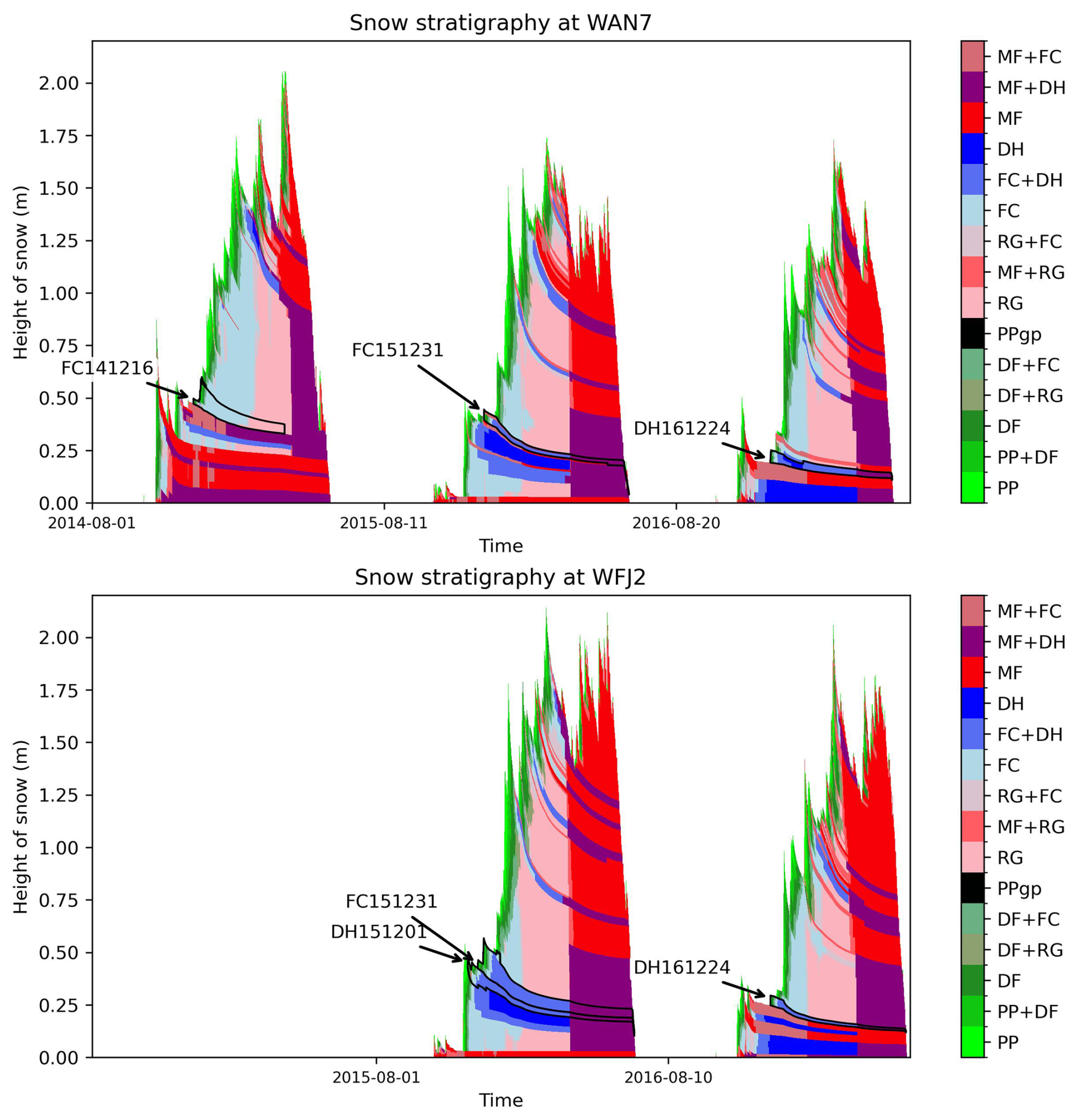
Figure 2 Simulated snow stratigraphy winters 2014–2015, 2015–2016 and 2016–2017 at the Wannengrat site (WAN7), and for winters 2015–2016 and 2016–2017 at the Weissflujoch site (WFJ2). The outlines of the weak layers considered in this study are highlighted by black lines.

To compare critical cut lengths derived from simulated snow stratigraphy with those measured in the field using PSTs, the corresponding weak layers must be first identified in the simulated profiles. Each observed weak layer is characterized by its burial date, which we used in combination with the deposition date in the Crocus simulations to establish matches. For each weak layer, a time window around the burial date is defined, plus one day and minus one week, to isolate candidate layers in the model. This window is refined if too many layers fall within it. A match is considered satisfactory if the simulated and observed weak layers agree in grain type, burial depth, and surrounding layer characteristics (e.g., crust presence). This approach was successful for all weak layers except SH150124, which the Crocus model could not reproduce. In total, 54 critical cut lengths were retained for comparison.

3 Results

In this section, we first established an empirical fit (i.e. a power law) describing the relationship between the min-cut ζ and density, both derived from 3D images of snow samples (see Sect. 2.3.1). This relationship is refined to account for differences between grain types using morphological descriptors specific to the Crocus snow model, namely the sphericity and SSA.

Then, we focus on the relationship between the min-cut ζ (estimated via the previous parameterization) and the fracture energy w_f using a linear relationship. To do so, we estimate the weak layer fracture energy using the PST dataset: the WEAC model is provided with the critical cut length measured with PSTs, for both observed and modelled profiles. Knowing the critical cut length and the entire profile, the model allows us to trace back to the corresponding fracture energy of the weak layer. With these pseudo-observations, we can relate w_f to the min-cut.

Eventually, we evaluate the whole parameterization of w_f as a function of density and grain morphology and its relevance to model the critical cut length in advanced (WEAC) or simple (Heierli) slab models.

3.1 Min-cut parameterization using 3D images of snow microstructure

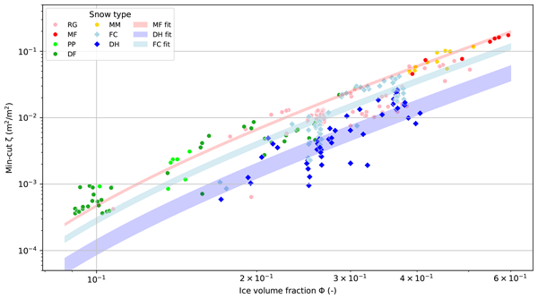
Figure 3 shows the min-cut as a function of the ice volume fraction and grain type. The min-cut increases with ice fraction ϕ, following a power-law relationship. The min-cut theoretically becomes zero below the percolation threshold (i.e. the critical ice fraction at which ice bonds first form a continuous network across the system). Therefore, this power-law relationship, often found for snow properties (e.g. Védrine et al., 2025), must account for a percolation threshold ϕ_t. In addition, for a given density, faceted crystals and depth hoar are characterized by a lower min-cut compared to other grain types. Therefore, an empirical fit should both account for density and grain type. We chose the following multiplicative form:

$$\begin{array}{}\text{(4)}& \mathit{\zeta }=f\left(\text{grain type}\right){\left({\displaystyle \frac{\mathit{\varphi }-{\mathit{\varphi }}_{\mathrm{t}}}{\mathrm{1}-{\mathit{\varphi }}_{\mathrm{t}}}}\right)}^m\end{array}$$

with ϕ_t and m parameters to be fitted, and f a scaling factor depending on grain type.

To ensure a smooth transition between grain types and to provide a physically meaningful description of the microstructural determinants of the min-cut, the scaling factor f is defined as a continuous function of microstructural descriptors. Here, we use the two microstructural descriptors employed by the Crocus model to characterise snow types: sphericity Ψ and specific surface area (SSA) s. Since grain types in Crocus are defined over specific intervals of these two variables (as reported in Table A1 in Appendix A), the fitting procedure accounts for these ranges, making this part of the parameterization dependent on the Crocus grain-type classification.

We used a logistic function for f and expressed the min-cut ζ as:

$$\begin{array}{}\text{(5)}& \mathit{\zeta }={\displaystyle \frac{\mathrm{1}}{\mathrm{1}+\exp \left(-{\mathit{\alpha }}_{\mathrm{0}}-{\mathit{\alpha }}_{\mathrm{\Psi }}\mathrm{\Psi }-{\mathit{\alpha }}_{\mathrm{s}}s-{\mathit{\alpha }}_{\mathrm{\Psi }s}\mathrm{\Psi }s\right)}}{\left({\displaystyle \frac{\mathit{\varphi }-{\mathit{\varphi }}_{\mathrm{t}}}{\mathrm{1}-{\mathit{\varphi }}_{\mathrm{t}}}}\right)}^m\end{array}$$

A least-square minimisation yields the following parameters: α₀ = −2.51, α_Ψ = 6.51, α_s = 0.16 kg m⁻², α_Ψs = −0.40 kg m⁻², ϕ_t = 0.04, and m = 2.7. Figure 3 shows the fitted relationships (Eq. 5) across the range of sphericity and SSA represented in the Crocus model for three grain types: melt forms (MF), faceted crystals (FC), and depth hoar (DH).

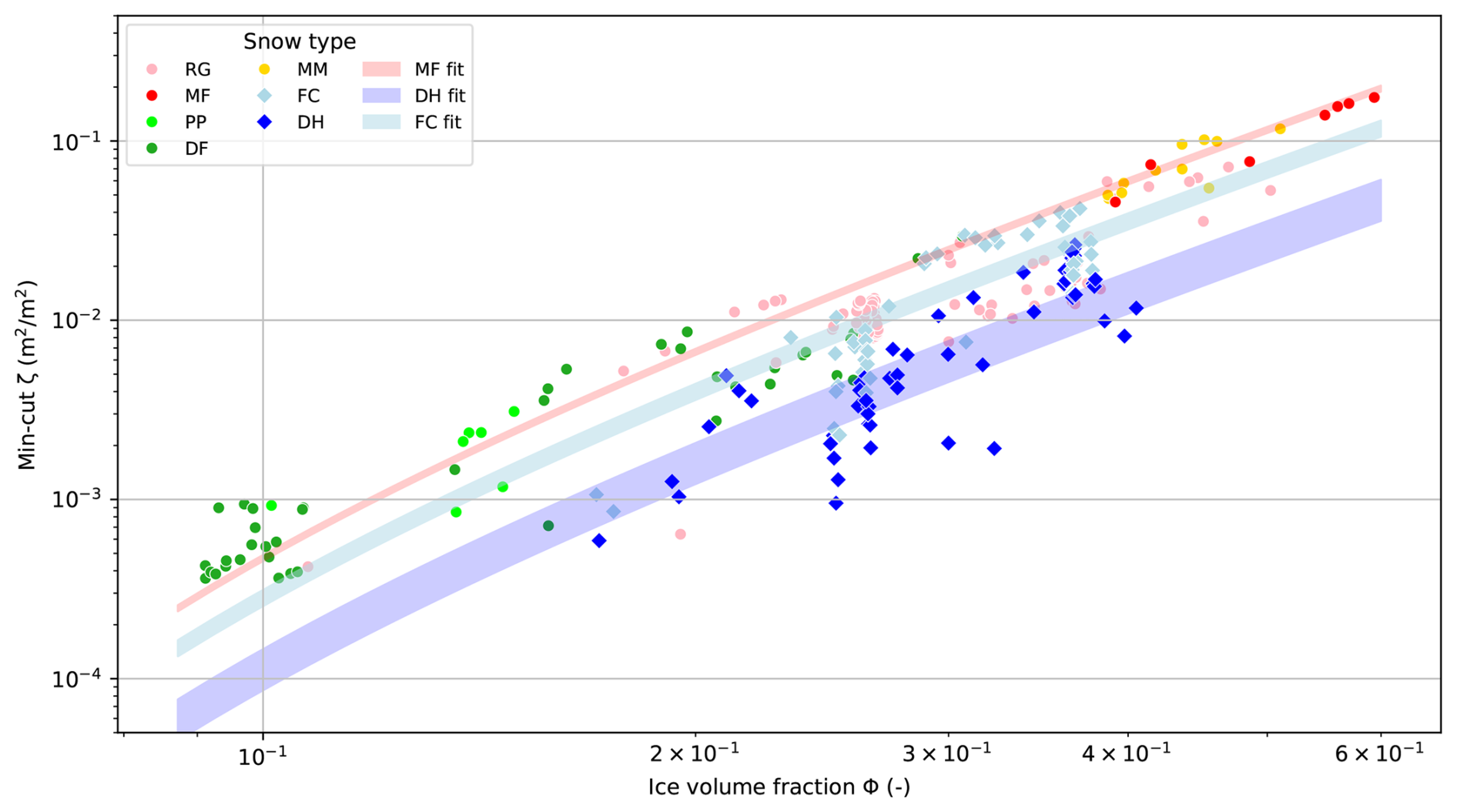
Figure 3 Min-cut ζ (m² m⁻²) as a function of the ice volume fraction (–) for all snow samples. Colors are used to differentiate between grain types and typical weak layers grain type are displayed with diamond markers. The colored shaded areas displays the application of the final parameterization Eq. (5), to the range of sphericity and SSA for melt forms (MF) in red, faceted crystals (FC) in light blue and depth hoar (DH) in dark blue.

3.2 Weak layer fracture energy parameterization

In this section, we estimate the relationship between the weak layer fracture energy w_f and the min-cut ζ. Using the WEAC model (Sect. 2.1.1), we invert the critical cut length from PSTs to derive w_f (dominated by mode I, see Sect. 2.1.1) from both observed and simulated snow profiles. These estimates are then compared to the min-cut ζ predicted using Eq. (5). To compute ζ, we used either manually measured density combined with the range of SSA/sphericity values associated to the observed grain type (see Table A1 in Appendix A), or the modeled density, SSA and sphericity from the corresponding weak layer in the Crocus profile.

3.2.1 Evaluation of simulated snow stratigraphy

Prior to using the modeled profiles with observed values (i.e., critical cut length from PST), it is necessary to verify that the main characteristics of the stratigraphy are accurately represented in the simulated profiles.

Figure 4 displays the modeled versus measured (a) slab density, (b) height of the slab, (c) weak layer density and (d) the weak layer grain types (in the form of a confusion matrix), for each time when PST data are available for both sites and for multiple tested weak layers.

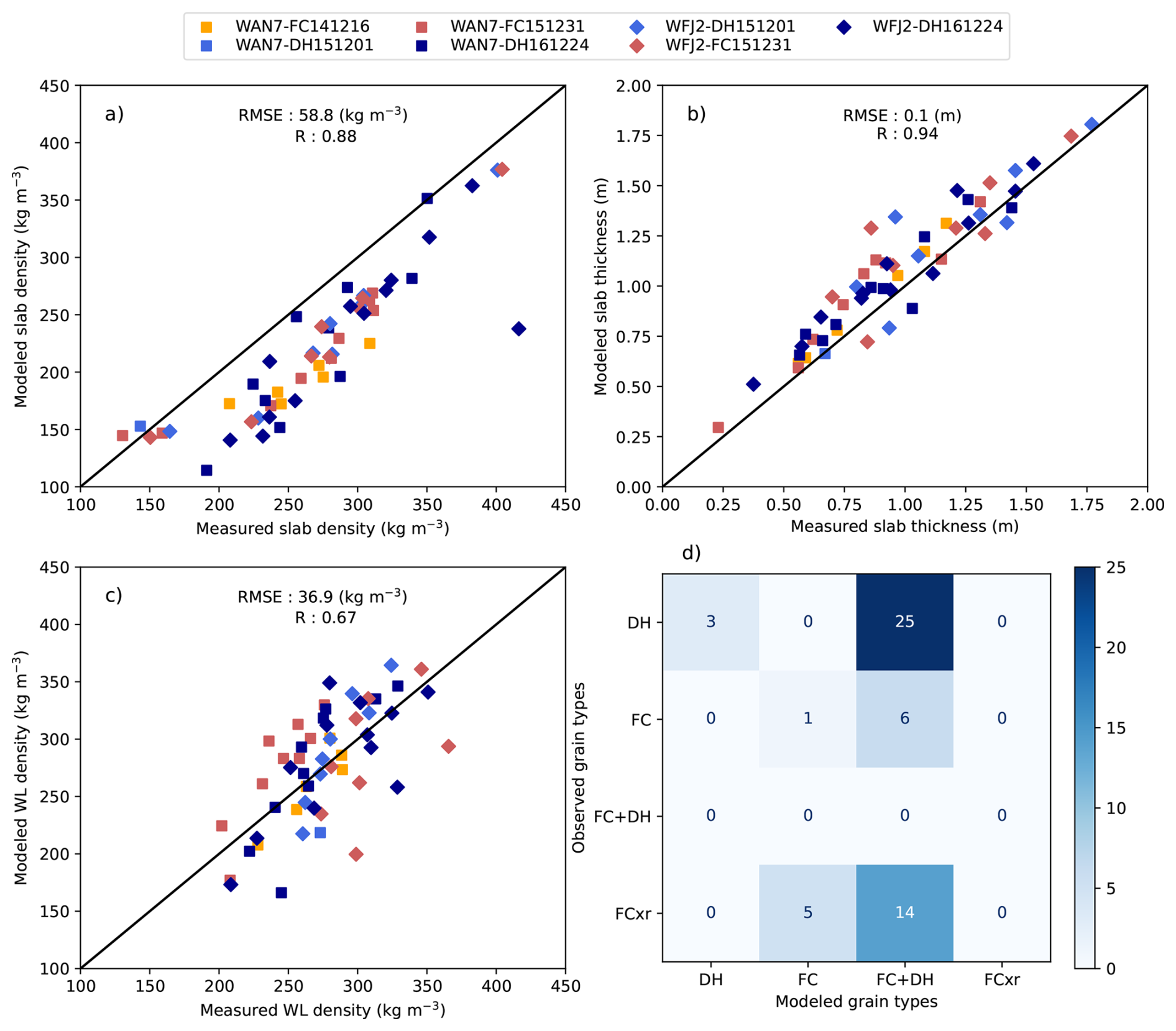
Figure 4 Comparison of (a) modeled to measured mean slab density ρ_sl, (b) slab thickness D_sl, (c) weak layer density ρ_wl and (d) the confusion matrix of the weak layer grain type based on Fierz et al. (2009) nomenclature. Modeled properties were taken from Crocus simulations while measured properties come from manually observed snow profiles. Each colors correspond to a specific tracked weak layer, markers refers to the site of measurement.

Slab density is almost systematically underestimated in the simulated profiles, with a root-mean-square-error (RMSE) of 58.8 kg m⁻³. However, the high linear correlation coefficient (R) of 0.88 indicates that despite systematic errors, Crocus is capable of providing consistent slab densities for all profiles where PSTs were performed. Only one modeled profile (related to the weak layer DH161224 at site WFJ2) appears to be largely underestimated compared to the measurements in terms of slab density, with a measured slab density above 420 kg m⁻³ while the modeled one is below 250 kg m⁻³.

Unlike slab density, the slab height is mostly slightly overestimated, with a RMSE of 0.1 m. The correlation coefficient with the measured slab height reaches 0.94, which indicates a very consistent agreement.

The modeled densities of the weak layer show greater variability in errors, with no clear trend toward underestimation or overestimation. The RMSE is approximately of 36.9 kg m⁻³, which is lower than that of slab densities, but with a lower correlation coefficient of 0.67 indicating a more dispersed and less consistent agreement for this variable. This lower agreement is not surprising, given, on the one hand, the difficulty in measuring thin and fragile snow layers, which leads to considerable uncertainty (Proksch et al., 2016), and, on the other hand, modeling errors of snow density and the matching of observed and modeled layers.

As illustrated in Fig. 4d, which shows the correspondence between the observed and modelled grain types at each measurement time and for each weak layer, we note that the majority of the measured weak layers were classified as DH or FC. Similarly, the layers modelled and identified as corresponding in Crocus are also classified as DH, FC or a mix of FC and DH. A significant proportion of the layers designated as DH, FC or FCxr in the observations are found in Crocus as FC+DH (i.e., 45 out of 53 layers). These discrepancies can be considered negligible for the purposes of this study, as all these grain types can be considered as weak layer and share similar characteristics.

Overall, the agreement between the measured and modeled characteristics of the slabs and weak layers is satisfactory and very close to that reported in Richter et al. (2019) using the SNOWPACK snow model. Although some systematic errors are present, the simulated profiles are close enough to be used with the measured critical cut length to estimate the weak layer fracture energy using the WEAC model.

3.2.2 Using observed and simulated snow profiles to estimate weak layer fracture energy

The w_f values retrieved from observed profiles range between 0.01 and 0.7 J m⁻². These scalar values comprise Mode I and Mode II contributions as retrieved by inversion of the WEAC model, and are predominantly Mode I-dominated (Mode I fraction above 85 % in most cases), as illustrated by the mode mixity reported for each PST in Fig. B1 of Appendix B. These w_f values correlate weakly with the min-cut estimated using the parameterization Eq. 5 and the measured weak layer densities and snow types (Fig. 5a). The linear correlation coefficients R ranges from 0.31 to 0.36 with a slope between 10.1 and 12.5 J m⁻². The use of modeled profiles and weak layer densities leads to values of w_f in the same range but with a better correlation to the min-cut (R = 0.48, slope of 15.2 J m⁻²) (Fig. 5b).

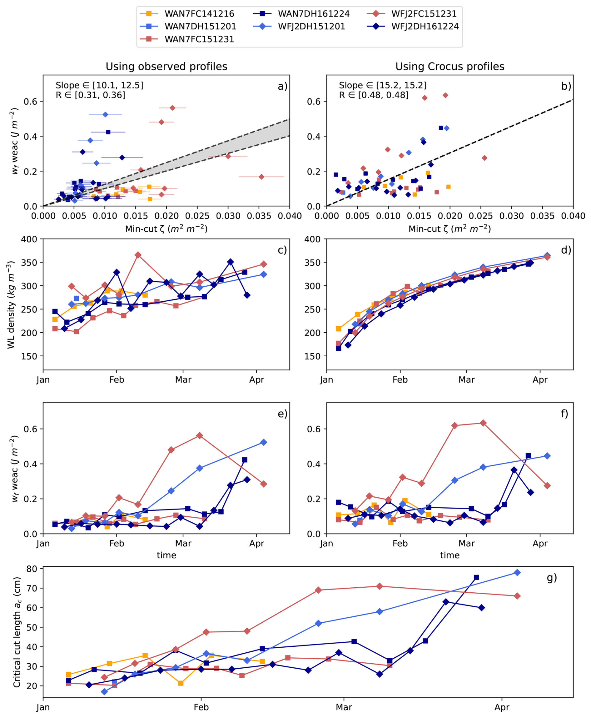
Figure 5 Comparison of the weak layer fracture energy (w_f) obtained using the WEAC model and min-cut ζ using Eq. (5) determined in Sect. 3.1 applied to observed profiles in panels (a), (c) and (e) and Crocus snow profiles in panels (b), (d) and (f). The colors and markers are associated with each followed weak layer. For each column, the evolution over time of the weak layer density (c, d), the w_f value estimated using the WEAC package (e, f), and the measured critical cut length (g) are also displayed. For observed profiles, slopes, scores and values of min-cut are presented along intervals, corresponding to the intervals of sphericity and SSA for each grain types in Table A1.

The differences in correlation coefficient between the use of measured and modeled profiles can be explained by the differences in the measured and modeled characteristics of the weak layer and the slab. The measured densities of the weak layer appear to fluctuate significantly over time, as is the case for the “WFJ2-DH161224” and “WFJ2-FC151231” layers (Fig. 5c). For these layers, measurements taken every two weeks may show significant increases in density of more than 50 kg m⁻³, followed by a decrease of the same order at the next measurement. These fluctuations in the density of the weak layer are physically implausible, since over time, under the effect of compaction, most snow layers tend to become denser. They are most likely the result of high measurement uncertainties, further addressed in Discussion section. The densities of the modeled weak layers follow a quasi-linear monotonic increase over time (Fig. 5d). Since the density of the weak layer is the main variable used to estimate the min-cut in the parameterization Eq. (5), these oscillations may explain some of the differences in correlation found between the use of measured and modeled profiles. In addition to these measurement uncertainties in the weak layer characteristics, there are also uncertainties in the estimation of the PST critical cut lengths (e.g., related to spatial variability of profiles, PST geometries and observers identification of weak layers), used in both cases (i.e., measured and modeled) to invert the WEAC model and obtain w_f.

All in all, assuming a linear relation between w_f and ζ and using Eq. (5), we can express w_f directly as a function of the density, specific surface area, and sphericity of the grains:

$$\begin{array}{}\text{(6)}& w_{\mathrm{f}}={\displaystyle \frac{A}{\mathrm{1}+\exp \left(-{\mathit{\alpha }}_{\mathrm{0}}-{\mathit{\alpha }}_{\mathrm{\Psi }}\mathrm{\Psi }-{\mathit{\alpha }}_{\mathrm{s}}s-{\mathit{\alpha }}_{\mathrm{\Psi }s}\mathrm{\Psi }s\right)}}{\left({\displaystyle \frac{\mathit{\varphi }-{\mathit{\varphi }}_{\mathrm{t}}}{\mathrm{1}-{\mathit{\varphi }}_{\mathrm{t}}}}\right)}^m\end{array}$$

with A = 15.2 J m⁻² for Crocus profiles and A = 11.2 J m⁻² for observed profiles, see Sect. 3.1 Eq. (5) for other parameters values. The robustness of these linear slopes are further assessed through a leave-one-out procedure, in which the slopes are recomputed by iteratively removing one weak layer per season. The resulting statistics (median, 10th and 90th percentiles) are reported in Table C1 in Appendix C.

3.3 Evaluation of modeled critical cut length

In this section, we evaluate the parameterization of the fracture energy w_f (Eq. 6) from several perspectives. First, we assess whether the prediction of the measured a_c is improved by using the proposed parameterization compared to a constant w_f. Next, we analyze the temporal evolution of predicted critical cut lengths from modeled profiles throughout a season. Finally, we examine the potential of predicted critical cut lengths to discriminate between weak layers and more stable layers within a profile.

3.3.1 Comparison of modeled and measured critical cut length

The values of a_c obtained from the measured profiles and a parameterized w_f (Fig. 6a) show an RMSE about 13.6 cm, with a linear correlation coefficient R of 0.49, indicating a moderate correlation between measured and modeled a_c (Fig. 6a). In contrast, using a constant w_f instead results in a higher RMSE of 14.5 cm and a lower correlation coefficient of 0.40 (Fig. 6b).

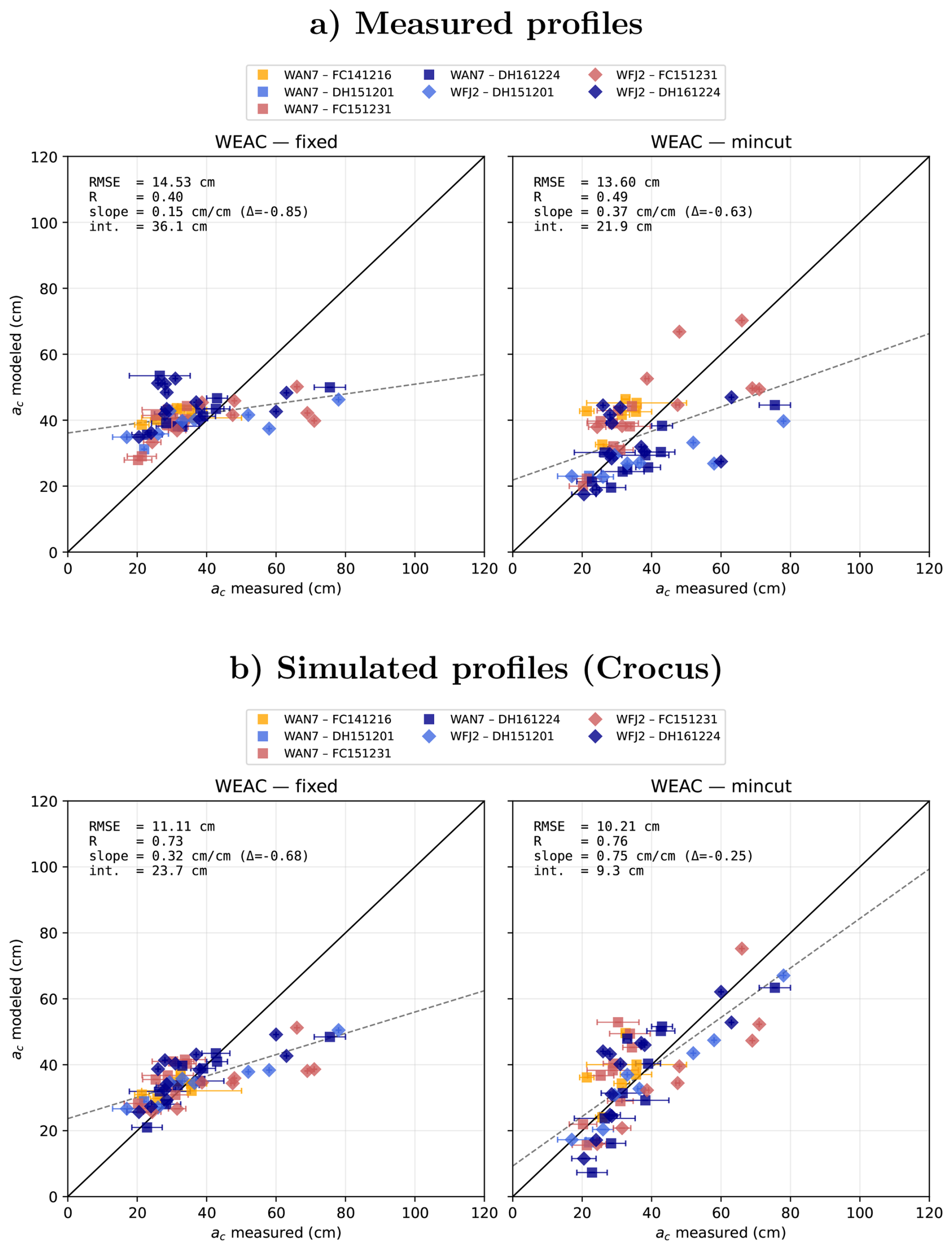
Figure 6 Comparison of the measured and predicted critical cut length a_c for a weak layer fracture energy w_f either constant or parameterized using the min-cut derived parameterization Eq. (5). The comparison is performed using input profiles observed (a) or simulated with Crocus snow model (b). The WEAC model is used to derive a_c. Uncertainties in measured critical cut length are displayed as horizontal error bars, vertical error bars corresponding to the range of a_c values obtained using the intervals of sphericity and SSA (reported in Table A1 in Appendix A) assigned to observed weak layers.

The slope of the 1:1 regression line and its intercept provide an indication of how well the modeled a_c values reproduce the full range of measured values. In the case of a fixed w_f, the slope is particularly low (0.15 cm cm⁻¹), reflecting a failure to capture the observed variability in a_c. The use of a parameterized w_f better captures this variability and improves the overall agreement with measurements.

Similar results are found using the simulated profiles (Fig. 6b). With a parameterized w_f, the RMSE is 10.2 cm and the correlation is 0.76, slightly above the scores with measured profiles. Indeed using a constant w_f slightly degrades the results (RMSE = 11 cm, correlation = 0.73), though the scores remain better than with the parameterized w_f on measured profiles (Fig. 6a). However, predicted a_c values obtained with a constant w_f remain strongly bounded, covering only a limited range of the observed values. This is particularly evident from the deviation from the 1:1 slope, which reaches −0.68 cm cm⁻¹ for profiles using a fixed w_f, indicating a substantial underestimation of the a_c variability, while this deviation is reduced to −0.25 cm cm⁻¹ when using a parameterized w_f. Surprisingly, using simulated profiles systematically yields better prediction of a_c compared to using observed profiles in the pit the PST were conducted. The possible reasons comprise the measurement uncertainties, in particular that of the weak layer density, whose impact on the estimation of w_f and the min-cut has been shown to be substantial in Sect. 3.2.2.

3.3.2 Time evolution of critical cut length

For each tracked weak layer (except WAN7-DH151201), Fig. 7 shows the temporal evolution of a_c over the winter season, comparing modeled and measured critical cut lengths.

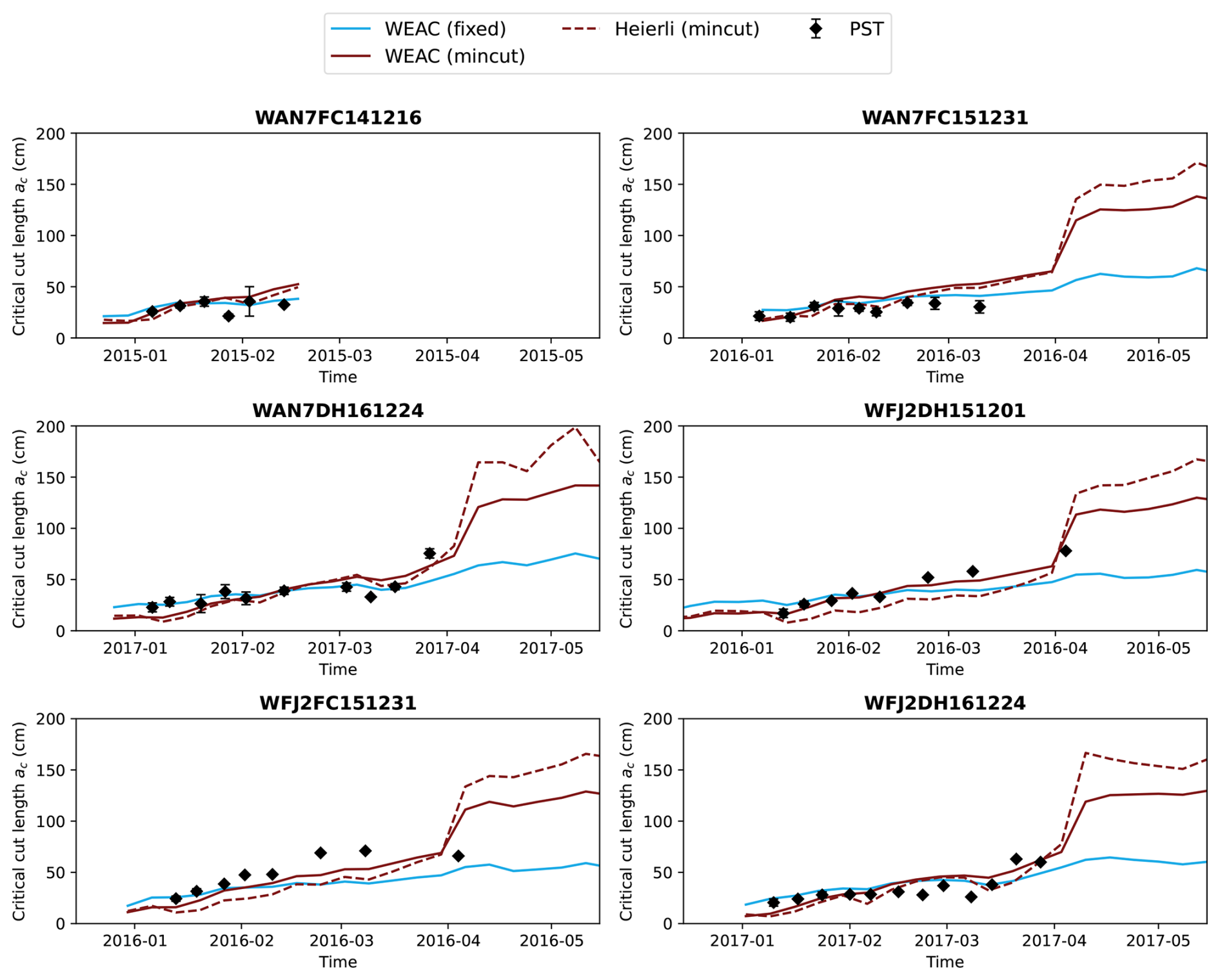
Figure 7 Time series of critical cut length (cm) for each of the weak layers tracked. The black diamonds with errorbars represent values measured using the PST. The critical cut length using the WEAC (continuous line) and Heierli (dashed line) models is displayed with the weak layer fracture energy estimated using either a fixed (blue line) or the linear relationship with the parameterized min-cut (Eq. 5) established in Sect. 3.2 (darkred line). The modeled critical cut lengths are calculated using Crocus snow profiles.

With a parameterized w_f, modeled a_c values most often fall within or close to the range of field measurements (±10 cm), with only slight and non-systematic biases: a minor overestimation for layer “WAN7-FC151231” and a minor underestimation for “WFJ2-FC151231”. Errors are fairly evenly distributed throughout the season, and the progressive stabilization of weak layers is correctly reproduced, including in the late season (end of March and April) for layers exhibiting this behaviour in PSTs, such as “WAN7-DH161224” and “WFJ2-DH151201”. The modeled temporal evolution is stable, showing no oscillations or abrupt peaks, consistent with the observed gradual stabilization of all weak layers over the course of the season.

In contrast, models using a fixed w_f frequently underestimate a_c values from spring onwards (March), as observed for layers “WFJ2-FC151231” and “WFJ2-DH151201”. While early-season results are broadly comparable to those obtained with a parameterized w_f with similar temporal evolutions and no systematic bias, the fixed-w_f approach produces only a weak increase in a_c toward the end of the season (less than 5–10 cm), failing to capture the pronounced stabilization reproduced by the parameterized models. This stabilization generally occurs in early April, coinciding with a period of substantial wet metamorphism of the snowpack (see Fig. 2).

3.3.3 Using critical cut length to identify weak layer in snow profiles

Figure 8 shows simulated (left) and measured (right) snow profiles on three dates: 6 January 2015, at site WAN7 in the first column, 10 February 2016, at site WFJ2, and 17 March 2017, at site WAN7. These dates were selected to span each season and each site at different times of the winter season.

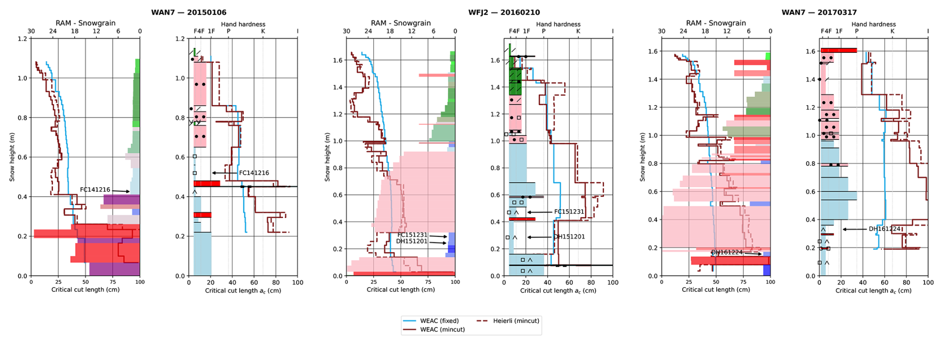
Figure 8 Modeled (left) and observed (right) snow profiles for three dates at different sites: 6 January 2015, and 17 March 2017, at the Wannengrat (WAN7) site, and 10 February 2016, at the Weissflujoch (WFJ2) site. The colors indicate the grain types, and rectangle dimension, the thickness of each layer, their resistance to penetration for the modeled snow profiles, and their hand hardness for the measured snow profiles. For each layer and each profile, the critical cut length using the WEAC (continuous line) and Heierli (dashed line) models is displayed with the weak layer fracture energy estimated using either a fixed (blue line) or the linear relationship with the parameterized min-cut (Eq. 5) established in Sect. 3.2 (darkred line). For each profile, the identified position of the weak layers is displayed either as measured or estimated using the deposition date in the case of modeled snow profiles as described in Sect. 2.3.3.

First, the WEAC and Heierli models using the min-cut parameterized w_f (darkred lines) predict similar evolution of a_c along a profile (measured or simulated). It is generally minimal near the surface, increasing slowly with depth, with local minimums and maximums generally located in similar areas.

These evolutions of a_c along the profile are consistent with the fact that near the surface (i.e. and generally early in the season) the layers are not very dense and therefore relatively weak despite the low weight above them. While presenting a low a_c, they are not typically weak layers since the thin and soft slab above is generally too fragile to support the bending induced by the weak layer failure. Deeper down, or later in the season, the layers become denser, even wet, and gain cohesion, becoming for the most part more resistant to failure. However, locally, thin layers with lower resistance due to lower density and/or cohesion may be present. These are the weak layers that are sought after, generally faceted crystals and deep or surface hoar, as these are failure layers found in avalanches (Schweizer et al., 2003; van Herwijnen and Jamieson, 2007) (blue and dark blue colors on the model profiles, square marker and hat on the obs profiles). Note that we focus here solely on one criterion, the onset of crack propagation and do not account for failure initiation, which may be very unlikely for deeply buried weak layers.

It can be seen that these weak layers are indeed those with the most pronounced local minima of a_c, with the other types of snow surrounding them generally having higher a_c values. These local minima are particularly pronounced at the end of the season, for example in the observed and modeled profile of “WAN7-20170317”. They can be seen on the observed profile at depths of 1.10 m, then 0.98 and 0.35 m, where there are corresponding local minima (i.e., a direct decrease of 10–30 cm in a_c). On the modeled profiles, they are visible at depth of 0.9, 0.8, 0.5 and then 0.15 m. These local minima are also visible to a lesser extent on the WFJ2-20160210 profile at 1.05 and 0.3 m (observed profile) and 1 and 0.3 m (modeled profile). Ultimately, with the exception of the “FC151231” layer on the observed profile, all of the weak layers tracked and annotated from the measured and modeled profiles stand out as local minima. Although these layers do not constitute absolute minimums across the entire profile (i.e., the top of the profile has lower values), the critical cut length emerges in these examples as a relevant indicator for highlighting weak layers.

In contrast, although the overall shape of the a_c profile obtained with WEAC using a fixed w_f is similar, it lacks pronounced local minima and instead exhibits a progressive, monotonic increase in critical cut length, rarely exceeding 60 cm. As a result, the sensitivity of the slab–layer configuration to propagation onset is nearly identical regardless of whether the layer consists of melt forms or depth hoar, as illustrated by the profile “WAN7-20170317” around 0.5 m depth. This suggests that the fixed w_f approach fails to capture a discriminating microstructural property of a weak layer, which is instead accounted for by the parameterized w_f derived from the min-cut approach.

4 Discussion

4.1 Deriving fracture energy parameterization at layer scale from microscopic measurements of snow samples

We estimated the fracture energy of snow by relating it to parameter of snow layers that are both available from observations and models, through a parameterization developed from microstructural properties measured using X-ray microtomography. A central contribution of this work is the use of the min-cut. This approach builds partly on the idea introduced by LeBaron and Miller (2014) and is in line with research seeking to relate macroscopic mechanical variables to microstructural properties derived from microtomography. For example, Köchle and Schneebeli (2014) used finite-element simulations and multiple tomographic images to infer macroscopic properties such as the elastic modulus, while Sundu et al. (2024) similarly developed a parameterization of the effective elastic tensor of snow. More recently, Schöttner et al. (2026) combined tomographic images with neural-network methods to predict compressive strength and stiffness.

In the present study, we rely on an extensive microtomography dataset covering a broad range of snow types and densities, from precipitation particles at around 75 kg m⁻³ to melt forms up to 550 kg m⁻³, as shown in Fig. 3. This approach avoids the use of discontinuous parameterizations and provides a unified relationship (Eq. 6) valid across all snow types. The fitting procedure, a weighted least squares, yields a percolation threshold ϕ_t = 0.04, corresponding to a snow density of approximately 35 kg m⁻³. This value lies slightly below the range of the snow dataset used, yet remains close to the density range of naturally deposited fresh snow (30 to 40 kg m⁻³, Helfricht et al., 2018), for which a non-zero min-cut is expected. It should also be noted that the characterization of different min-cut between grain types (for a given density) is captured in the fit using prognostic variables specific to the Crocus model, namely SSA and sphericity. This part of the parameterization is therefore model-dependent and would need to be recalibrated using the corresponding variables and their associated value ranges for any other snowpack model to which it is transferred. The power-law component (i.e. density dependency), by contrast, is model-independent. Ultimately, this parameterization may be applied consistently across all layers of a snow profile (whether field-measured or simulated with Crocus) to compute w_f. This value can then be incorporated into a slab model to estimate the critical cut length.

Two key assumptions are made in our approach. First, we assume that the min-cut can be related to a macroscopic quantity, in particular the snow density. Results presented in Sect. 3.2.2 support this assumption and show that for a given density, layers composed of faceted crystals and depth hoar consistently exhibit lower min-cut values, with depth-hoar layers showing the lowest values among the grain types considered (see Fig. 3). These observations motivated the introduction of additional microstructural descriptors (grain sphericity and SSA) into the parameterization, such that the min-cut scales depending on grain type and decreases specifically when the grain type approaches the characteristics of faceted crystals and depth hoar. These findings align with Schöttner et al. (2026) results, who show that density captures the first-order variability of mechanical properties such as stiffness and compressive strength, while microstructural attributes are essential for distinguishing the mechanical behavior of persistent weak-layer grain types, including faceted crystals and depth hoar.

The second assumption is that the min-cut scales linearly with fracture energy. While this assumption is not directly supported by experimental studies or fracture theory, the min-cut quantifies the minimum amount of microstructure that must be disconnected, and it may reasonably be interpreted as a first-order proxy for fracture energy. Under this interpretation, it could be viewed as a lower-bound estimate, as additional energy dissipation associated with microstructural rearrangement, local stabilization mechanisms, or non-optimal fracture paths is not accounted for. This hypothesis could not be confirmed, as the linear fit between min-cut and fracture energy provided only a moderate correlation at most (R = 0.48; see Fig. 5).

Several factors may explain the relatively low correlations obtained in the linear regression between w_f and min-cut, some of which may be related to measurement and modeling uncertainties (discussed in the following section of the discussion), but could also point to a lack of complexity in the proposed parameterization, as the min-cut alone may not fully capture the variability of fracture energy. Nonetheless we demonstrate the clear advantages of using this relationship rather than a constant w_f, as shown by the results in Sect. 3.3.1 and discussed in a further section.

4.2 Measurement and modeling uncertainties

Using modeled rather than measured slab and weak layer characteristics consistently showed better performance in the correlation between w_f and the min-cut (Fig. 5) and to the R and for RMSE scores for critical cut lengths (Fig. 6). Lower scores obtained with measured profiles, and the weak correlations between w_f and the min-cut, can partly be attributed to uncertainties in measuring and modeling slab and weak layer properties, primarily density.

The temporal evolution of these properties is shown in Fig. 5. While the modeled weak layer density increases smoothly over time, the measured density fluctuates unrealistically by about ±50 kg m⁻³ between 2-week intervals. These values were obtained using density cutters or tubes (Richter et al., 2019), which are known to have uncertainties up to 10 % (i.e. when compared to micro-CT measurements), increasing for layers only a few centimeters thick (concerning most of the followed weak layers), generally overestimating low-density and underestimating high-density snow layers (Proksch et al., 2016). Added to this uncertainty are the observer's subjective choices regarding the delineation of the different layers, as well as the hectometric variability of the snowpack, all of which make it difficult to monitor the different layers consistently and reliably over the course of a season. Similarly, the evolution of slab characteristics (aggregating all layers) shows greater oscillations in measured than in modeled profiles. Figure 5 also indicates that Crocus densities are systematically lower than measured ones, an already documented model bias such as in Quéno et al. (2016), that could be explained by an underestimation of compaction processes. Critical cut lengths from PSTs, used in both modeled and measured cases, also carry uncertainty, similarly to those related to the weak layer. They result from the observer's choice of cut, spatial metric variability that can be pronounced for thin layers such as weak layers that can be seen on uncertainties in Figs. 6 and 7, and by design in the PST protocol for large values approaching the 150 cm column length.

Because the WEAC model depends on numerous parameters (e.g., density, layer thickness, measured critical length), these uncertainties compound, potentially by adding up one another (i.e., underestimating critical length while overestimating weak layer density) thereby applying an increased penalty to the scores.

All of these uncertainties, whether they concern measurements or modeling, make it difficult to estimate a relationship between w_f and the min-cut and probably explain the better scores obtained when using modeled profiles, which, although biased, remain temporally stable and internally consistent. These considerations underline the need for improved field measurement techniques for weak layers and continued refinement of parameter evolution laws in macroscopic snow models.

4.3 On the added-value of the w_f parameterization

The parameterization of w_f remains satisfactory in several respects, even though the correlations between w_f and the min-cut values presented in Sect. 3.2.2 (Fig. 5) are only moderate. First, the values of w_f inferred through inversion of the WEAC model lie between 0.01 and 0.7 J m⁻² for weak layers. This range is consistent with previous studies, which generally report weak-layer fracture energies between 0.01 and approximately 1.5 J m⁻² (Schweizer et al., 2011; Bergfeld et al., 2023). This range is also consistent with the total energy release rate values where mode I is dominant (including collapse and in-plane shear), of 0.4–0.8 J m⁻² as reported in Adam et al. (2024), which was retrieved by performing PSTs over buried surface hoar. This agreement provides confidence that the parameterization derived from our fit will provide physically realistic values of w_f.

Second, the temporal evolution of w_f derived from our simulations is consistent with the observations of Schweizer et al. (2016), who documented time evolutions of mechanical properties (i.e. elastic modulus and specific fracture energy) in weak layers. Their results show that fracture energy is generally not expected to decrease over time because sintering increases bonding between grains, except under strong temperature-gradient. A similar pattern is visible in Fig. 5, where many weak layers exhibit relatively stable w_f values around 0.1 J m⁻² for several weeks before increasing toward the end of the season. This late-season increase is consistent with the stabilization trends described by Schweizer et al. (2016).

The results in Sect. 3.3.1, comparing modeled and measured critical cut lengths, further highlight the benefits of using the w_f parameterization developed in Sect. 3.1 and 3.2.2, rather than using a constant w_f. For both observed profiles (Fig. 6) and simulated profiles (Fig. 6), statistical scores (i.e., R, RMSE) are better when the parameterized w_f is used.

In addition, employing a constant w_f severely restricts the range of critical cut lengths that the WEAC model can reproduce, preventing any values below 20 or above 60 cm. These findings indicate that w_f plays a major role in the dynamics of critical cut length modeling within the WEAC model, and emphasizes the importance of even slight variations during the season, as well as its increase at the end of the season acting the stabilization of the weak layer.

Finally, although acceptable scores can still be obtained when using a constant w_f (Fig. 6), it remains applied to pre-identified weak layers. The narrow range of critical cut lengths produced under a constant w_f limit the model's applicability for detecting weak layers within full profiles as in Fig. 8 or for tracking their stabilization over time as in Fig. 7. Overall, these results clearly demonstrate the advantages of using a parameterized w_f over a constant value within the WEAC model.

A qualitative comparison with Richter et al. (2019) (based on a stress-strength approach) reveals consistent results across several aspects. The stratigraphic profiles of a_c (their Fig. 9) exhibit a pattern similar to those obtained here, with a progressive increase of a_c with depth and local minima clearly associated with weak layers. The temporal evolution (their Fig. 11) is likewise comparable: critical cut lengths remain relatively stable over most of the season before increasing substantially towards its end, consistent with the progressive stabilization of the profile. Similarly, Richter et al. (2019) report degraded performance when using manually observed profiles instead of simulated ones, in line with the score differences observed here between observed and Crocus-simulated profiles. This overall consistency across two independent modelling frameworks is encouraging and further supports the physical coherence of the present results. Part of this agreement between the strength-based approach of Richter et al. (2019) and the energy-based framework of this study could be theoretically motivated. Indeed, cohesive-zone formulations (Park and Paulino, 2013) may bridge the two approaches by removing the crack-tip stress singularity and relating the effective fracture toughness to the constitutive properties of the weak layer (e.g., its strength, elasticity, and effective thickness) (Gaume et al., 2026). Under the small-scale yielding assumption (i.e., when the process zone remains small compared to the elastic characteristic length of the slab–weak-layer system), such stress-based formulations and the linear elastic fracture mechanics approach are expected to agree (Gaume et al., 2026).

Overall, the approach proposed in this study builds on the state-of-the-art WEAC slab model and a min-cut parameterization derived from a large and diverse set of snow microstructure samples, suggesting more robust transferability to a broader range of snowpack conditions compared to Richter et al. (2019). The inherent limitations of the linear relationship between min-cut and w_f are, discussed in Sect. 4.5.

4.4 Comparing two slab models of different complexity

In the study sections dedicated to the evaluation of the parameterization of w_f, two anticrack models of different complexity were compared: Heierli's model and the state-of-the-art WEAC model. The two models differ primarily in their treatment of slab and weak-layer deformation. The WEAC model explicitly accounts for the deformation of a stratified slab as well as that of the weak layer. Its geometry is free on both sides, designed specifically to represent the configuration of a PST. In contrast, the Heierli model is based on an idealized geometry in which a homogeneous slab is supported on one side, and describes the deformation of slab sections that are no longer supported by the weak layer. Owing to these simplifications, the Heierli model depends solely on the weak layer fracture energy w_f and does not require additional parameters describing the weak layer that are in any case difficult to obtain through measurements or modeling.

It should be noted that in this study, the Heierli model is implemented using an elastic modulus taken from the formulation of Gerling et al. (2017) recently modified by Bergfeld et al. (2023), with an equivalent elastic-modulus expression derived from the mode-I formulation of WEAC (see Sect. 2.1.2). These additions enhance the representation of layering effects, even though they are not explicitly included in the deformation model. Such additions are absent from previous implementations described by Heierli et al. (2008), Schweizer et al. (2011), Reuter et al. (2015), and they allow the Heierli model to get results that are more consistent with those of the WEAC model. Despite the differences in complexity and underlying assumptions, the temporal evolution of a_c for weak layers (Fig. 7) and the profiles of a_c for selected dates (Fig. 8) show similar results for the two models.

Ultimately, although the overall performance of the WEAC model is slightly superior to that of the Heierli model (notably in Fig. 7), the discrepancies remain small. This suggests that either model could be used in operational applications based on snow-model outputs, particularly given the relative simplicity of the Heierli formulation and the smaller number of parameters required for its implementation.

4.5 Limitations and perspectives

The work presented in this article, although making the best use of the tools and datasets available, is subject to a number of limitations that are worth discussing. The parameterization of w_f using the min-cut as an intermediate variable substantially reduces the dimensionality of the problem as it integrates both density and morphological effects into a single physically interpretable quantity. This allows calibration over a much larger and more diverse dataset than the PST dataset alone, improving robustness across snow types. The w_f min-cut relationship is nonetheless validated on a restricted set of FC and DH weak layers, though its application to full stratigraphic profiles (Fig. 8) yields physically consistent a_c values across layer types, suggesting reasonable potential broader applicability.

Regarding the limitations of the w_f dataset itself, it is mainly restricted to Mode-I-dominant conditions, as illustrated in Fig. B1b). However, following the work of Adam et al. (2024), who performed a large number of PSTs under various geometric configurations and loading conditions, demonstrate that such mode mixity conditions (i.e. crack propagation dominated by mode I, approx. > 75 %) are representative of typical avalanche-triggering configurations (including “remotely”) with slope angles of 0 to 40. Nonetheless, the snowpack in a 30 to 40° actual avalanche start zone may differ from a research site in terms of snow stratigraphy (i.e. due to wind redistribution, settlement, radiation, and spatial variability). This represents a limitation, although it is common in most research on snowpack stability, due to the difficult access and monitoring conditions in these areas.

We also note that the PST dataset covers only a limited range of weak layer types, namely faceted crystals (FC) and depth hoar (DH). The fact that surface hoar (SH) is not represented in Crocus limits the validation of the parameterization for this grain type, and no weak layers composed of fresh snow, such as precipitation particles (PP) or decomposing and fragmented particles (DF), are included in the dataset. It should further be noted that the two study sites, located approximately 3 km apart in Switzerland, are representative of Alpine snowpacks, which may differ substantially from other snowpack types, such as maritime snowpacks found in parts of the mountain ranges of North America, or continental and Arctic snowpacks characteristic of higher-latitude environments.

It would therefore be valuable to extend the validation of the proposed parameterization by applying the method to other PST datasets, in order to test the transferability and robustness of the relationship across different snowpack types (oceanic, continental, and Arctic snowpacks), a larger range of grain types including surface hoar SH, non-persistent weak layers such as PP and DF, and ideally PSTs performed on non-weak layers as a reference, as well as on geometric configurations favoring greater mode mixity. The proposed w_f parameterization should thus be regarded as an effective, PST-based formulation, subject to the limitations of the dataset on which it was built, rather than as an intrinsic mechanical law. Its operational applicability to any avalanche release zone remains to be demonstrated, particularly because the test design of the PST (i.e., the introduction of an unsupported part of the slab) may not be representative of the processes involved in avalanche formation on steep slopes.

Ultimately, the critical cut length modeling proposed in this study remains insufficient to assess crack propagation on its own, as it addresses only one specific stage: the onset of crack propagation, assuming that failure initiation has already occurred. As illustrated in Fig. 8, which shows the evolution of a_c along a snow profile, particularly low critical cut lengths are found near the surface. However, near-surface fresh snow may lack sufficient bonding to constitute a cohesive slab (Schweizer et al., 2003), and crack propagation may be prevented by slab fracture even when the computed critical cut length is small (Gaume et al., 2015). This highlights the need to combine the present indicator with additional mechanical criteria in future work: a strength-to-stress ratio for failure initiation, thereby satisfying the coupled criterion of Leguillon (2002) and a tensile strength criterion for crack arrest (e.g. Gaume et al., 2015). Such a combined analysis would connect the present work to operational triggering likelihood, and would contribute to providing more effective tools for operational risk management.

5 Conclusions

The principal objective of this study was to develop a framework for estimating the onset of crack propagation, suitable for integration into macroscopic snowpack models such as Crocus to improve dry-snow slab avalanche hazard assessment. A key challenge addressed herein concerns the estimation of parameters that cannot be measured directly, such as the weak layer fracture energy w_f used in models like those of Heierli and WEAC (see Sect. 2.1).

Building upon the state-of-the-art WEAC model and a dataset of nearly 300 tomographic images of diverse snow samples, we developed a new approach to estimate w_f from microstructural properties. First, a power-law relationship was established between bulk snow density and microstructural properties (specifically, the number and size of ice bonds) combined through the min-cut indicator. While most snow types follow a common law, faceted crystals and depth hoar exhibit systematically lower min-cut values. This behavior is captured in the proposed relationship through a scaling coefficient that accounts for grain sphericity and specific surface area. Then, we used a multi-year field dataset from Richter et al. (2019), comprising time series of measured snow stratigraphy and corresponding weak-layer critical cut lengths derived from Propagation Saw Tests (PSTs) across two alpine sites. The continuous min-cut parameterization was compared to fracture energies w_f inverted from the WEAC model using both observed and modeled snow stratigraphies. A moderate correlation between min-cut and w_f was obtained under a linear fit, with improved agreement when modeled stratigraphy (from Crocus) was used. These findings are likely the result of both measurement and modeling uncertainties, as well as possible limitations in the explanatory capacity of the min-cut variable alone to fully capture w_f variability.

Despite these limitations, the derived relation between w_f and min-cut provides a consistent parameterization that links macroscopic snow properties (i.e., density, grain sphericity, and SSA) to PST-derived effective fracture energy (dominated by mode I). When incorporated into two anticrack models of differing complexity (WEAC and Heierli), the proposed parameterization improved the prediction of critical cut lengths compared to a constant w_f. Despite comparable RMSE and correlation scores, it produced a_c values that are more consistent across the full range of measured critical cut lengths, while accounting for microstructural differences. This allows the parameterization to better discriminate the layers most sensitive to propagation onset within a snow profile, and to capture the temporal evolution of this sensitivity over pre-identified weak layers.

Overall, the proposed parameterization represents a step toward bridging microstructural snow physics and avalanche forecasting using macroscopic snowpack models. Its integration into snowpack models opens up the door to better predict dry-snow slab avalanches, whether for operational purposes or for assessing hazard evolution under changing climate conditions.

Appendix A: Sphericity and SSA intervals from Crocus snow model

Table A1 Table of the SSA (m² kg⁻¹) and sphericity (–) intervals from Crocus snow model associated with the grain type used in this study.

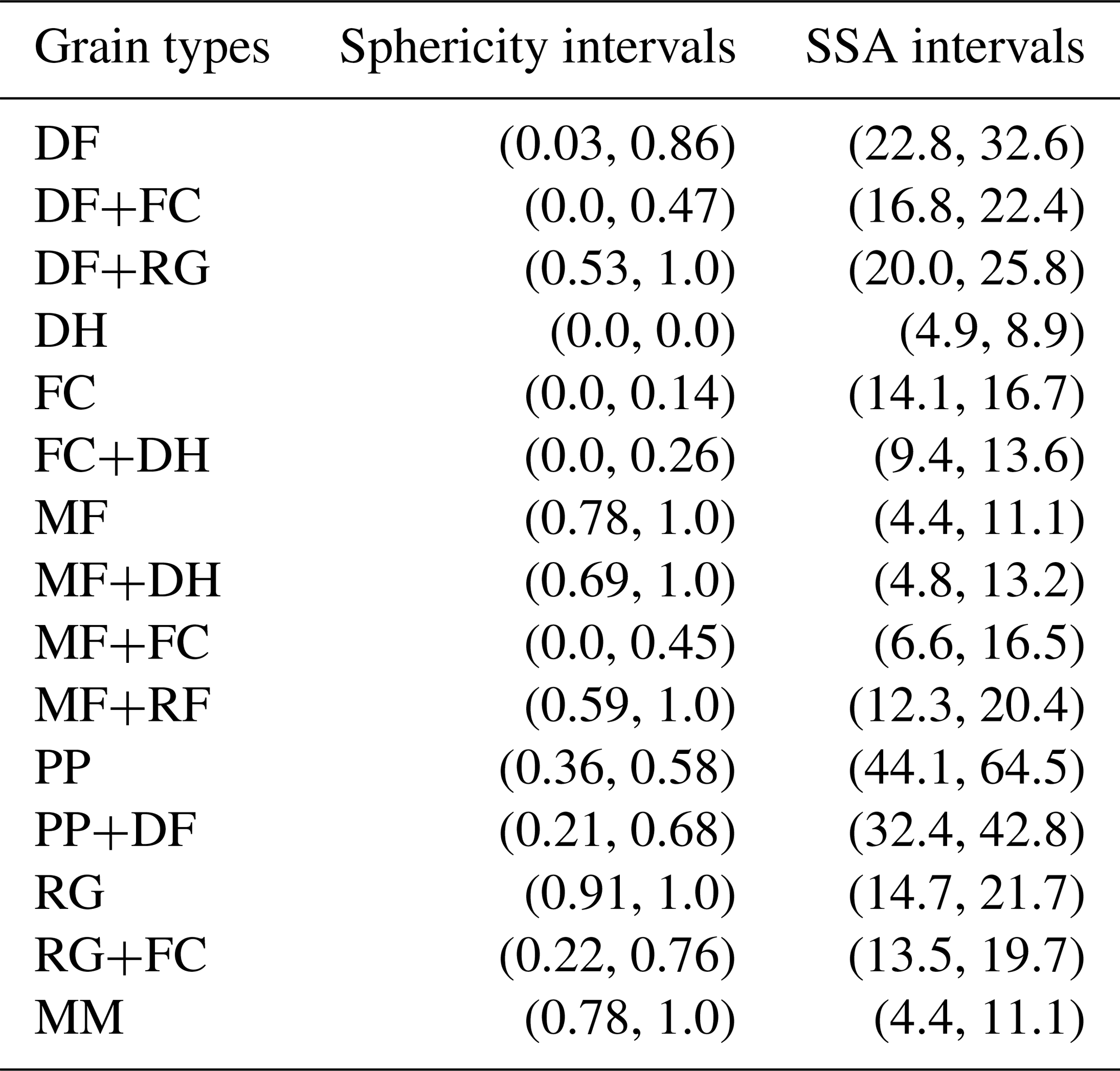
Table A1 associates grain types with sphericity and SSA ranges. These ranges are obtained from the 5th and 95th percentiles of the sphericity and SSA distribution for each grain type, using 60 years of the S2M reanalysis (Vernay et al., 2022) in the French Alps massifs using version 9.0 of the Crocus snowpack model (Lafaysse et al., 2025). They correspond to the distribution of SSA and sphericity as modelled by Crocus and are therefore specific to it. These ranges are used throughout the article, where fracture energies w_f are calculated using manually observed profiles, for which we do not have access to the sphericity or SSA of the weak layers (see Sect. 3.2.2 and 3.3.3).

Appendix B: Mode mixity and sensitivity analyses of w_f to elastic modulus parameterization and weak layers thickness

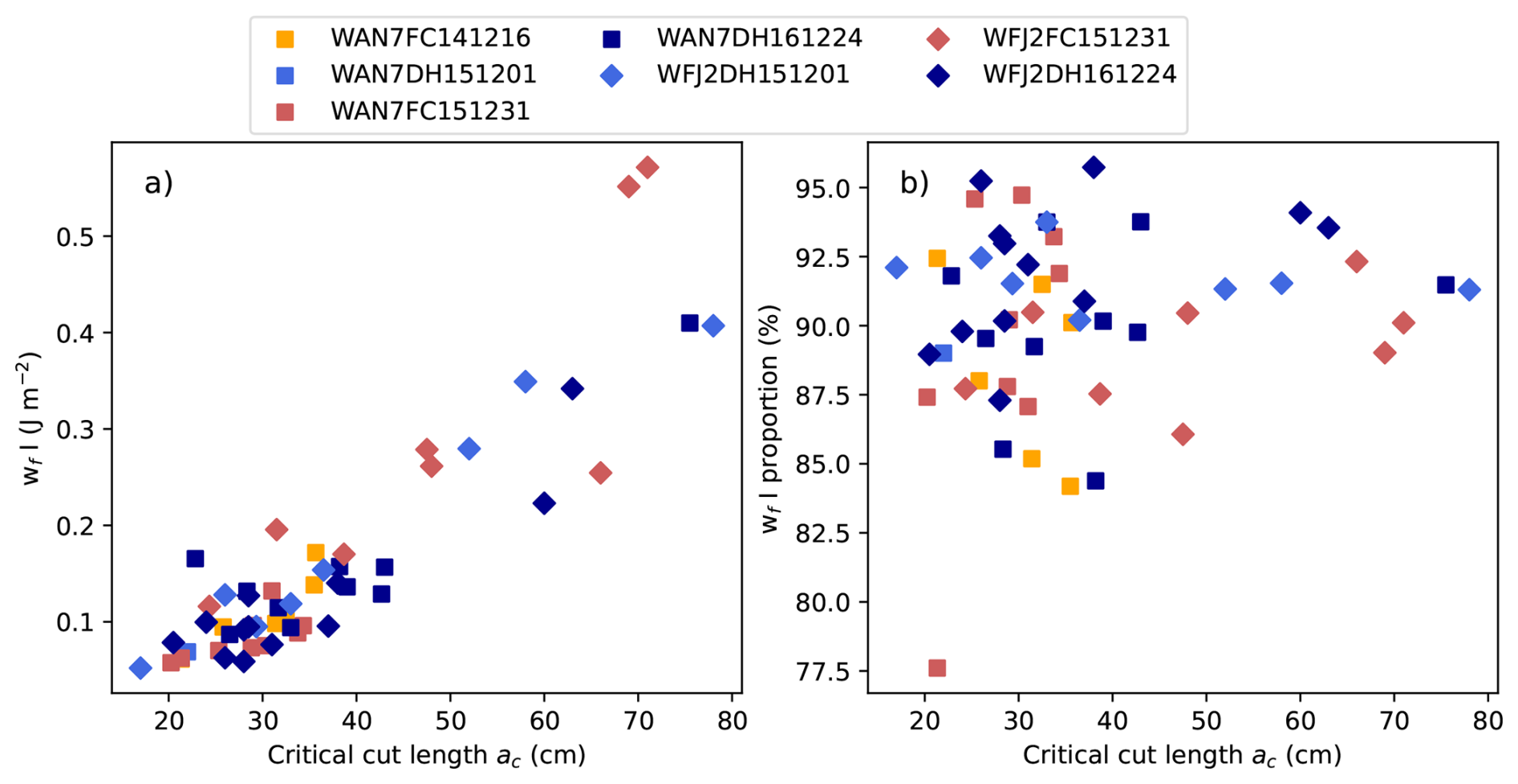
Figure B1 (a) Mode I w_f (J m⁻²) as a function of critical cut length for all layers and sites. (b) Proportion of mode I w_f as a function of critical cut length for all layers and sites.

In this appendix section, we report in Fig. B1a the mode I values of w_f as retrieved by inversion using the WEAC model, as a function of the critical cut lengths reported from the PSTs used in this study, for each weak layer at both monitored sites. Figure B1b shows the ratio of mode I to total fracture energy w_f (i.e., mode I + II).

Figure B2 shows the distribution of w_f values (mode I + II) for each weak layer at both monitored sites, as retrieved by inversion using the WEAC model with measured snow profiles (Fig. B2a) and profiles simulated with the Crocus model (Fig. B2b). For each type of snow profile used, the values are presented under different assumptions regarding the parameterization of the elastic modulus E used to compute those of both the slab and the weak layer (except for the fixed assumption at 0.15 MPa only applied to weak layer elastic modulus), as well as assuming either a fixed weak layer thickness of 30 mm or a thickness derived from the measured/simulated profiles. All values are plotted against the values of w_f retrieved using the set of hypotheses retained for the study, namely the E parameterization from Bergfeld et al. (2023) and a fixed h_wl at 30 mm as justified below.

A fixed weak-layer thickness of 3 cm was adopted to ensure methodological consistency between Crocus simulations and field-measured profiles. As discussed by Richter et al. (2019), layer boundaries in manual snow profiles are strongly observer dependent and often reflect apparent stratigraphic homogeneity rather than mechanical relevance, leading to manually identified weak layers spanning 20–30 cm. Similarly, layer aggregation in Crocus can produce weak layers up to 15 cm thick. In both cases, treating the full layer thickness as mechanically homogeneous appears physically inconsistent. Furthermore, as shown in Fig. B2, using measured or modeled thicknesses instead of a fixed value systematically yields larger inverted w_f values, frequently exceeding the range reported in the literature (0.01 to 0.7 J m⁻², see Sect. 4), and degrades both the w_f min-cut correlation and the agreement between modeled and measured critical cut lengths (not shown here). For the elastic modulus of the slab and weak layer (except for the fixed 0.15 MPa assumption applied to the weak layer), we used the density-based parameterization of Bergfeld et al. (2023), a slight revision of Gerling et al. (2017) derived from acoustic-wave measurements, which currently represents one of the most experimentally supported density-based relationships available.

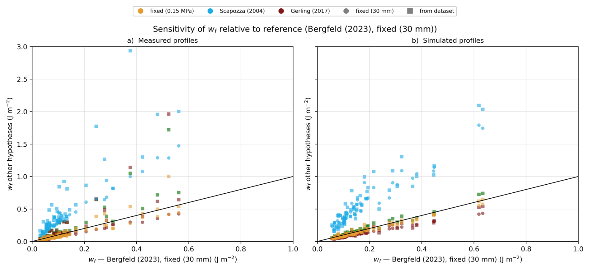
Figure B2 Sensitivity analyses of w_f for measured (a) and simulated profiles (b), showing the w_f values for all layers and sites of the study under different elastic modulus parameterizations: fixed (0.15 MPa) in orange, Scapozza (2004) in blue, Gerling (2017) brown and Bergfeld (2023) in green. Weak layer thickness h_wl assumptions are also displayed: fixed at 30 mm (circle markers) or derived from dataset profiles (square markers). These values are plotted against the w_f values obtained from the hypotheses retained for the study, namely using the modulus parameterization of Bergfeld et al. (2023) and a fixed h_wl of 30 mm. Note that the assumption of a fixed elastic modulus, E = 0.15 MPa, applies to the weak layer only. Under this assumption, the slab elastic modulus is determined using the formulation proposed by Bergfeld et al. (2023).

Appendix C: Leave-one-out fitting results between fracture energy w_f and min-cut ζ

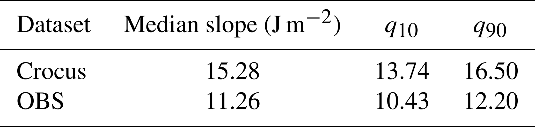
Table C1 reports the median and quantiles q₁₀ and q₉₀ of the linear slope computed between w_f and the min-cut, following a leave-one-out procedure. In practice, slopes are computed by iteratively removing one monitored weak layer at a time for a given season and site.

Table C1 Sensitivity of the fitted min-cut–w_f relationship to the leave-one-out (LOO) procedure. LOO was performed by recursively removing one weak layer at one site for a given season. Reported values correspond to the median fitted slope in J m⁻² together with the 10th and 90th percentiles obtained across all LOO realizations.