Modeling the Subglacial Sediment System of the Finnish Lake District Ice Lobe During Deglaciation

The systematic connection of glacial conditions in ice models with subglacial geomorphological observations has been limited by an inability to model subglacial sediment processes. The Finnish Lake District Ice Lobe (FLDIL) is a major  500 km long ice stream of the Fennoscandian Ice Sheet that has been interpreted as being oscillatory and re-advancing during the Younger Dryas. The FLDIL presents an opportunity to apply new model approaches in a situation of relative simplicity, with a well-preserved sedimentary record of its past subglacial hydrology and ice flow. With a recent model of the FLDIL subglacial hydrology as driver, we derive a sediment system model ensemble using the Graphical Subglacial Sediment Transport model (GraphSSeT). Model scenarios analyse the impact of varying sedimentary conditions, and resolve spatial and temporal variations in basal sediment thickness, sediment flux rate, grain size and detrital provenance. Our results show the development of a supply-limited system within 10 years characterised by strong seasonal cycles of winter gains from bed erosion, spring and summer losses from the mobilisation of basal sediment and autumn gains from deposition. Modelled at-outlet grain size also varies seasonally and would yield clastic varves, if deposited in a proglacial lake. The results define a submarginal zone of basal sediment depletion extending 40–60 km back from the terminus, in line with the modern-day sediment thickness.The mobilisation of an extensive blanket of sediment from this submarginal zone is proposed to form the Salpausselkä II ice marginal complex. Our model approach provides a template for the validation of subglacial hydrology models against sedimentary observables, opening a path to employ such constraints to study hard-to-observe modern and past subglacial hydrology and ice conditions.

1 Introduction

A well-constrained knowledge of the dynamic evolution of sediments in the subglacial environment is a significant factor to understand the development of the cryosphere (Andresen et al., 2024; Overeem et al., 2017), and the associated impacts on landscapes (Hepburn et al., 2024; Boulton et al., 2007), seascapes (Kirkham et al., 2024) and ecological and ocean systems (Cape et al., 2019; Meire et al., 2017; Chu et al., 2009). A significant challenge to developing this knowledge to a high level is the ability to quantitatively model the behavior of sediments under ice with sufficient spatio-temporal resolution to capture dynamic processes. The ability to accurately simulate geological and geomorphological observables is key to unlocking our ability to use sediments to constrain hard-to-observe subglacial hydrology systems under major ice sheets and in the past (Licht and Hemming, 2017; Ojala et al., 2022; Lunkka, 2023).

From foundational concepts (Shreve, 1972; Röthlisberger, 1972; Walder and Fowler, 1994; Boulton et al., 2007), subglacial hydrology models have evolved increasingly sophisticated representations of the hydrology system interconnected with ice sheet dynamics (Hewitt, 2011; Flowers, 2015; Werder et al., 2013). The integration of advanced hydrology modelling approaches, e.g. the Glacier Drainage System model (Werder et al., 2013), with the latest generation of ice sheet model codes, e.g. the Ice-sheet and Sea-level System Model (Larour et al., 2012) has spurred a revolution in the application of subglacial hydrology models at-scale and with more realistic forcings and higher spatial and temporal resolution (Ehrenfeucht et al., 2023; Dow et al., 2022; Hepburn et al., 2024; Sommers et al., 2023). In turn, these developments in subglacial hydrology models have opened the door to better understand the impact of hydrology on sediments and thus new potential to connect the cryosphere with its sedimentary consequences (Delaney et al., 2019, 2023; Delaney and Adhikari, 2020; Aitken et al., 2024).

A recently developed approach to the latter problem, the Graphical Subglacial Sediment Transport (GraphSSeT) model represents the subglacial hydrology system as a graph, permitting flexible characterisation of network properties, and the ability to track sediment mobilisation, transport, and deposition driven by channelised water flow (Aitken et al., 2024). As well as resolving sediment flux, GraphSSeT tracks key sediment characteristics such as grain size and detrital provenance, that are routinely observed in the sedimentary record (Licht and Hemming, 2017; Vorren, 1977; Lunkka et al., 2021; Hovikoski et al., 2023).

GraphSSeT has previously been applied to suites of synthetic models (Aitken et al., 2024) but its capacity to resolve more complex systems has not been comprehensively tested. This work applies this approach to a realistic catchment-scale simulation of the Finnish Lake District Ice Lobe of the Fennoscandian Ice Sheet (Hepburn et al., 2024). This region is a compelling test case due to its relatively simple ice sheet structure, its dynamic seasonal hydrology, and widespread, well-exposed and well-studied morpho-lithogenetic landforms and sedimentary observables with which to compare the findings (Lunkka et al., 2021; Palmu et al., 2021). A model-ensemble is used to develop a knowledge of the subglacial sedimentary system factoring in variations in sedimentary initial conditions, and the results are compared to the subglacial and proglacial landscape and its sediment characteristics.

2 The Finnish Lake District Ice Lobe

The Finnish Lake District Ice Lobe (FLDIL) is a significant component of the former Fennoscandian Ice Sheet (FIS). The FIS is remarkable for the formation of a series of large ice lobes during the Late Weichselian deglaciation, particularly in association with the Younger Dryas stadial (12.9–11.7 cal. ka), the last cold period marking the transition from the Late Pleistocene to the Holocene (Palmu et al., 2021; Alley et al., 2003; Naughton et al., 2023). Geomorphological and geochronological evidence indicate that, while the main deglaciation of the FIS was paused during the Younger Dryas, the ice margin exhibited significant and complex behaviour involving rapid oscillations, retreats and re-advances across many areas of Fennoscandia (Lunkka et al., 2021; Hughes et al., 2023). The migration of the ice lobe margins was evidently diachronous, varying in both time and space (Saarnisto and Saarinen, 2001; Lunkka et al., 2021; Hughes et al., 2023). Regions that experienced substantial ice-margin re-advances during the Younger Dryas preserve some of the best-developed landforms in the FIS area, such as the Salpausselkäs ice-marginal complexes in southern Finland.

The Salpausselkäs were formed at the ice margin in front of the Baltic Sea Ice Lobe and the FLDIL, which terminated in the Baltic Sea Basin during deglaciation (Boulton et al., 2001; Lunkka et al., 2021). They consist of two sub-parallel main ridges, the Salpausselkä I and the Salpausselkä II, and the more scattered Salpausselkä III, which occurs only in the Baltic Sea Ice Lobe area. Today, the Salpausselkäs stand out from their surrounding landscape as elevated arcs (100 to 150 meter above sea level), hundreds of kilometres long, and comprising end moraine ridges, subaquatic fans and extra-marginal glaciofluvial deltas (Palmu et al., 2021; Lunkka, 2023).

Current understanding suggests that, in the FLDIL area, the Salpausselkä I was formed at around 12.5 cal. ka, with a maximum age of 13.3 ± 0.9 cal. ka (Saarnisto and Saarinen, 2001; Svendsen et al., 2004; Lunkka et al., 2021). The age of the Salpausselkä II is better constrained, as it is associated with the sudden drainage of the Baltic Ice Lake into the North Atlantic via the Kattegat-Skagerrak region at 11.6–11.7 cal. ka (Saarnisto and Saarinen, 2001; Johnson et al., 2022; Regnéll et al., 2025). This drainage occurred soon after the ice margin began to retreat north-northwest from the Salpausselkä II, providing an estimated age of 11.6–12.0 cal. ka for its formation (Saarnisto and Saarinen, 2001; Lunkka et al., 2021). Evidence for the drainage includes a series of ice-contact delta pairs, located ∼ 5 km up-ice from the Salpausselkä II, with a 26–28 m difference in delta-plain elevation (Lunkka, 2023). This abrupt event closely marks the termination of the Younger Dryas and the onset of the Holocene Epoch, and was followed by a collapse to an ice-free state in Fennoscandia by ∼ 9 cal. ka (Kleman et al., 1997).

The final phase of the FLDIL evolution has been the focus of recent studies aimed at understanding how the self-organisation of the subglacial hydrological network evolved and systematically generated landscape features such as murtoos (Ojala et al., 2019, 2021) and subglacial meltwater routes (Ahokangas et al., 2021; Dewald et al., 2022), which are linked to the transition from distributed to channelised subglacial hydrology (Hepburn et al., 2024).

The FLDIL is a compelling example with which to study both the subglacial hydrological system (Hepburn et al., 2024) and the associated sedimentary evolution, due to several characteristics: First, topographic relief is overall low and flat (Fig. 1a), lacking deeply incised glacial valleys or fjords, and therefore provides little topographic focusing of ice flow; second, the advance and subsequent ice margin retreat from the Salpausselkä II over the model region was relatively short-lived; third, there is an abundance of well-preserved glacial geomorphology including eskers and ice-marginal deposits (Fig. 1a); finally, these sediments and the bedrock geology beneath are well-mapped with high quality and openly available datasets, including sediment thickness maps (GTK Finland, 2025d) and grain-size analyses and geochronology studies (Vorren, 1977; Lunkka et al., 2021).

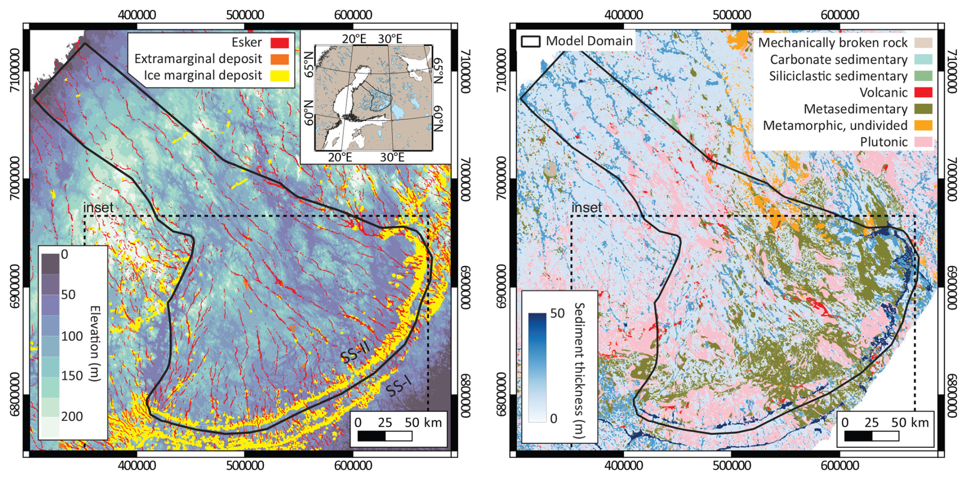
Figure 1 Overview map of the FLDIL region showing (a) surface topography (Danielson and Gesch, 2011) and glacial features (GTK Finland, 2025c), (b) surficial sediment thickness (GTK Finland, 2025d) and exposed bedrock geology, shown where sediment is absent (GTK Finland, 2025b). The dominant bedrock units comprise plutonic and metasedimentary rocks, with minor units for volcanic and other metamorphic rocks. The solid black line shows the model domain while the dashed box shows the extents of the maps shown in all other figures. Major ice marginal deposits are Salpausselkä I (SS-I) and Salpausselkä II (SS-II). The coordinate system is EUREF-FIN EPSG:3067.

For this study we frame our work with the following research questions:

1. Can the sub- to pro-glacial sediment dynamics of the FLDIL be well represented in a hydrology-forced sediment system model?

2. Can the sediment system model explain geological observables, including subglacial sediment thickness, and the characteristics and spatial distribution of ice-marginal deposits?

3. Can the comparison of geological observables with the sediment model outcomes help to better constrain ice sheet and subglacial hydrology system evolutions?

3 Methods

3.1 GlaDS and GraphSSeT

Our approach is grounded in the combination of a Glacier Drainage System (GlaDS) subglacial hydrology model (Werder et al., 2013), implemented in the Ice-sheet and Sea-level System Model (ISSM) (Larour et al., 2012; Ehrenfeucht et al., 2023) applied as forcing to the GraphSSeT sediment system model.

GlaDS resolves hydrological flow in two coupled components; an inefficient continuous sheet representing flow in a linked-cavity network (Walder and Fowler, 1994), and an efficient channelised flow, represented by semi-cylindrical channels, called Röthlisberger-channels, or R-channels (Röthlisberger, 1972). In the finite-element-method (FEM) model the sheet-flow is resolved over the elements while the channelised flow is resolved along element edges. Coupling between these components is achieved by equalising the pressure between the channels and the adjacent sheet (Werder et al., 2013).

In GlaDS, the R-channels evolve in time through a thermodynamic balance between expansion through melting versus closure by viscous ice-creep (Werder et al., 2013). The opening rate is driven by heat-transfer from turbulent water flow and changes in the pressure-melting point, and varies with changes in the hydraulic potential gradient, the rate of water flow, and the water pressure (see Eqs. 15 and 16 in Werder et al., 2013). The closing rate is driven by ice deformation proportional to Nⁿ where N is effective pressure, and n is the exponent in Glen's flow law, typically n= 3. In this study, the ice geometry is fixed, therefore channel evolution reflects the changing water flow and basal water pressure. With increased meltwater supply, mass conservation demands faster flow, in response to which channels will expand; in contrast decreasing water supply will cause slower flow, and channels will contract. Consequently, the conditions of pressurised high-velocity water flow needed to transport sediment may be quite variable through both space and time.

Taking a GlaDS model result as input, GraphSSeT translates the FEM mesh into a directed acyclic graph incorporating element edges and nodes, through which the channelised hydrology network is represented (Aitken et al., 2024). Edges carry the information for channelised flow including water flow rate, channel cross-sectional area and hydraulic potential gradient. Nodes carry the information of the ice geometry including bed elevation, ice thickness, effective pressure and basal ice velocity. In GraphSSeT elements are not included and the role of hydrologic sheet flow in sediment transport is not considered explicitly.

The GraphSSeT model (Aitken, 2024) involves several processes computed in order. First, the sediment transport capacity is derived based on the basal shear stress τ which is proportional to the square of the mean water velocity u_w in the channel. The transport capacity, in this case using the formulation of Engelund and Hansen (1967), is proportional to ${\mathit{\tau }}^{\mathrm{5}/\mathrm{2}}$ and the net effect is that transport capacity varies proportional to $u_{\mathrm{w}}^{\mathrm{5}}$. The transport capacity is grain size dependent, and is linearly inverse-proportional to d₅₀ (Engelund and Hansen, 1967), the median grain size of sediment to be transported. Other factors are small influences on transport capacity (Aitken et al., 2024). In the second step, sediment mobilisation from and demobilisation to the basal sediment layer is calculated. Here we consider the balance of sediment transport capacity versus sediment supply from upstream and local bed erosion, and the sediment available in the basal sediment layer (Delaney et al., 2019). If sediment supply from upstream is less than the transport capacity, this will lead to mobilisation from the basal sediment layer, so long as sediment is available. On the other hand, sediment supply exceeding transport capacity will lead to demobilisation to the basal sediment layer (Fig. 2). The third step considers transport at network-scale, which is managed to maintain the following conditions: sediment volume is always conserved; transport capacity is never exceeded; reasonable sediment velocity limits are never exceeded. In the last stage statistical distributions of grain size and detrital provenance are tracked on the network through volumetric-mixing equations. Detritus tracking is entirely passive, however, the evolving grain size can have significant impacts on transport capacity and so model evolution, where transport-capacity limited (Aitken et al., 2024).

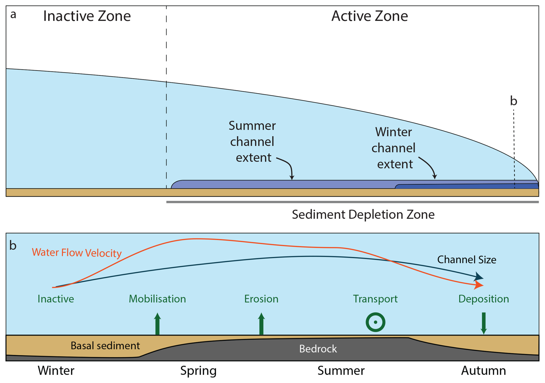
Figure 2 Schematic of the GraphSSeT model setup showing the glacial-hydrological scenario. (a) A side-on section through the FLDIL with ice in light blue, basal sediment in brown and R-channel extents in darker blues for summer and winter conditions – channel height is not to scale. Active hydrology exists near the margin, and is driven back and forth through a ∼ 60 km wide active zone by seasonally variable conditions. In this active zone the sediment becomes depleted. (b) Seasonality of behaviour near the margin, at the location indicated by a dotted line in (a), showing hydrology conditions (channel section area and water velocity) and sediment dynamics through time. R-channels show low-flow conditions in winter, high-velocity flow in still enlarging channels during spring, large channels with reduced flow velocity during summer, and low-velocity flow in contracting channels during autumn. These changes in channel geometry and flow rate over time are reflected in sediment cycling, typically with phases including inactivity during low flow, mobilisation of basal sediment during periods of increasing flow followed by erosional supply from the bedrock, transport of sediment supplied from upstream, and deposition to the basal sediment layer where supply exceeds transport capacity.

3.2 Model Design and Implementation

Paleoproxy-based reconstructions indicate that climate and climate seasonality impact was not uniform through the North Atlantic and Europe during the Younger Dryas, with different timing and character (Lie and Paasche, 2006; Schenk et al., 2018). This demonstrates its complexity, including ocean-atmospheric coupling, which is difficult to master from spatio-temporal perspective. Although these variations may have had very significant impacts on the hydrology and sediment systems, for this case study we seek to understand variable sediment dynamics using a single hydrology forcing. Therefore, we restrict analysis to the subglacial hydrology derived using the climate forcing applied in Hepburn et al. (2024, 2023). In their work, the FLIDL extent is representative of the end of the Younger Dryas stadial (∼ 12 cal. ka), when complex seasonality is thought to have given way to warmer climate with similar seasonality to present-day conditions (Mangerud et al., 2023).

Hepburn et al. (2024) ran a FLDIL-GlaDS simulation for 10 000 d (27.3 years) to describe subglacial drainage within the FLDIL. The model geometry comprised an initially parabolic ice surface that was allowed to relax over 10 000 years, and a representative basal topography created by subtracting sediment thicknesses from a modern terrain. The FLDIL-GlaDS model was forced using a modern precipitation record for the region, a modern temperature record depressed by 15 °C, and an elevation dependant lapse rate of 7.5 °C km⁻¹. A quadratic function was used to estimate monthly temperature variability (Wake and Marshall, 2015), and a positive degree day scheme used to calculate total monthly melt rates (van den Broeke et al., 2010). Melt was integrated within randomly distributed catchment areas and routed to the bed via 2500 moulins. A spatially uniform basal velocity of 150 m yr⁻¹ was imposed, and the FLDIL-GlaDS model ran with an adaptive timestep between 90 s and 1 h.

For input to the GraphSSeT model, we use the last 10.5 years of the model run. To reduce compute load, the 10.5 year model evolution is divided into beginning, middle, and end segments each of 3.5 years duration (Fig. 3). GlaDS model outputs were extracted at ∼ 4 d intervals and for each, the channel water flux and channel area were spatially filtered to reduce abrupt changes in conditions between edges and ensure network connectivity (Fig. 3).

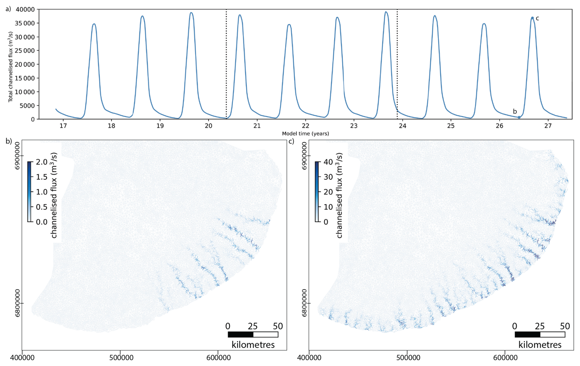
Figure 3 The hydrology model forcing showing (a) integrated channelised water flux through the last 10.5 years of the FLDIL-GlaDS model run (Hepburn et al., 2024). Dotted lines indicate beginning, middle and end legs (b) channelised water flux at end-winter conditions (26.4 years) (c) channelised water flux in peak flow conditions (26.7 years).

The GraphSSeT geology model involves sediment in active transport, a basal sediment layer accessible to hydrology-forced mobilisation, and an underlying bedrock released into the transport system by glacial erosion (Fig. 2). In the standard implementation, the basal sediment layer is variable in thickness between zero and an imposed upper limit (1 m here). In this work, we introduce a mixed-bed mode where thick sediment accumulations are available for mobilisation, but we retain the maximum limit for demobilisation, necessary to avoid potential for runaway sediment accumulations. In the standard implementation, the sediment cover of the area (Fig.1) is considered as bedrock, requiring glacial erosion, while in the mixed bed model it is considered as basal sediment, able to be mobilised by hydrology. Glacial erosion potential is defined with a quadratic formula (see;  Herman et al., 2021) using the basal velocity of 150 m yr⁻¹ from the GlaDS model, giving erosion potential of ∼ 6 mm yr⁻¹.

For each ∼ 4 d GlaDS model output interval, the GraphSSeT implementation runs with constant forcing. GraphSSeT time steps were between 1 h and 1 d duration, adapting to the basal sediment thickness (H), targeting $\max (\mathrm{d}H/\mathrm{d}t)=H/\mathrm{2}$. At the end of the GlaDS interval, the graph is reformed, including any changes in the directions of edges and/or locations of outlet nodes and updating the forcing parameters. State variables including sediment thickness, active sediment flux density, grain size and detrital properties are transferred to the new graph. Summary model outputs are derived at the end of each GlaDS model output interval, and full model outputs are exported for selected intervals identified at inflections in the total channelised water flux (Fig. 3).

3.2.1 Model Scenarios and Initial Conditions

We tested three model scenarios with initial conditions that represent different possible glacial-sedimentological conditions. These scenarios are selected to test key controls on sediment dynamics, and to assess ability to explain observations from the FLDIL region.

1. low-H: this scenario considers a low initial sediment thickness. This scenario represents a sediment-free former glacial margin, with only a brief period of subglacial sediment accumulation. Sediment thickness begins in a low-sediment state with randomly distributed values (5± 2.5 cm). New sediment is developed from erosion, with a constant erosion potential over the entire domain, in line with the constant basal velocity used in Hepburn et al. (2024). Sediment accumulates over a 20-year steady state run in winter hydrology conditions, yielding a maximum thickness of ∼ 11 cm.

2. high-H: this scenario considers a higher initial sediment thickness. In comparison to the low-H scenario, this scenario has a more prolonged period of subglacial sediment accumulation from erosion, but otherwise is identical. A 150-year steady state run in winter hydrology conditions yields a maximum initial thickness of ∼ 60 cm.

3. Mixed-bed: this scenario considers spatially variable sediment coverage, representing the sedimentary remnants of a previous glaciation with similar geometry. Unlike the previous scenarios, the sediment thickness begins with the modern-day sediment thickness and is then initialised with a 20 year steady-state run in winter conditions as before. In our driving hydrology models, the topography surface represents the modern-day surface minus the sediment thickness (Hepburn et al., 2024). Here we wish to test the impact of higher sediment availability under consistent forcing, therefore we do not adjust topography for the sediment thickness. Sensitivity testing done in Hepburn et al. (2024) showed that the change in elevation from removing the sediments does not drive major change in the hydrology system.

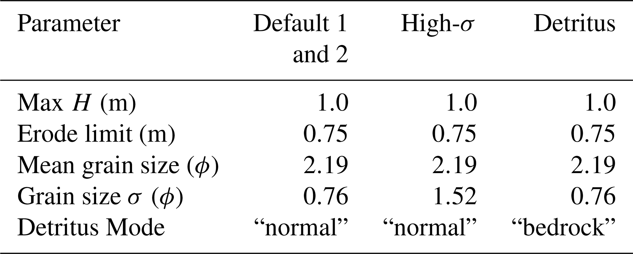
Table 1 Selected model parameters for different run modes. Default 1 and 2 used the same parameters

3.2.2 Ensemble Trees

Our model design uses ensemble trees (Fig. 4) to develop statistical robustness of the outcome while reducing the compute cost. For each initial condition we have a separate tree, each with three subtrees. The main subtree is the “default” mode, with two subordinate subtrees using a) the “bedrock” detrital tracking mode and b) increased grain size variability, High-σ (Table 1). The “bedrock” detritus mode does not affect sediment dynamics – the difference is that the “bedrock” detrital provenance is retained after cycling through the basal sediment layer, whereas in the “normal” detritus mode the detrital provenance is reset to “basal” when deposited. High grain size variability, in principle, will provide a more dynamic model evolution due to its impact on transport capacity. For each subtree a cascade of runs is completed for each leg, yielding at least four results for the “default” subtree, and two for the others (Fig. 4). GraphSSeT is stochastic with respect to sediment grain size and also network-scale transport conditions. Although computational limitations preclude a large ensemble, we run two realisations for the default setup, to indicate the impact of this stochasticism.

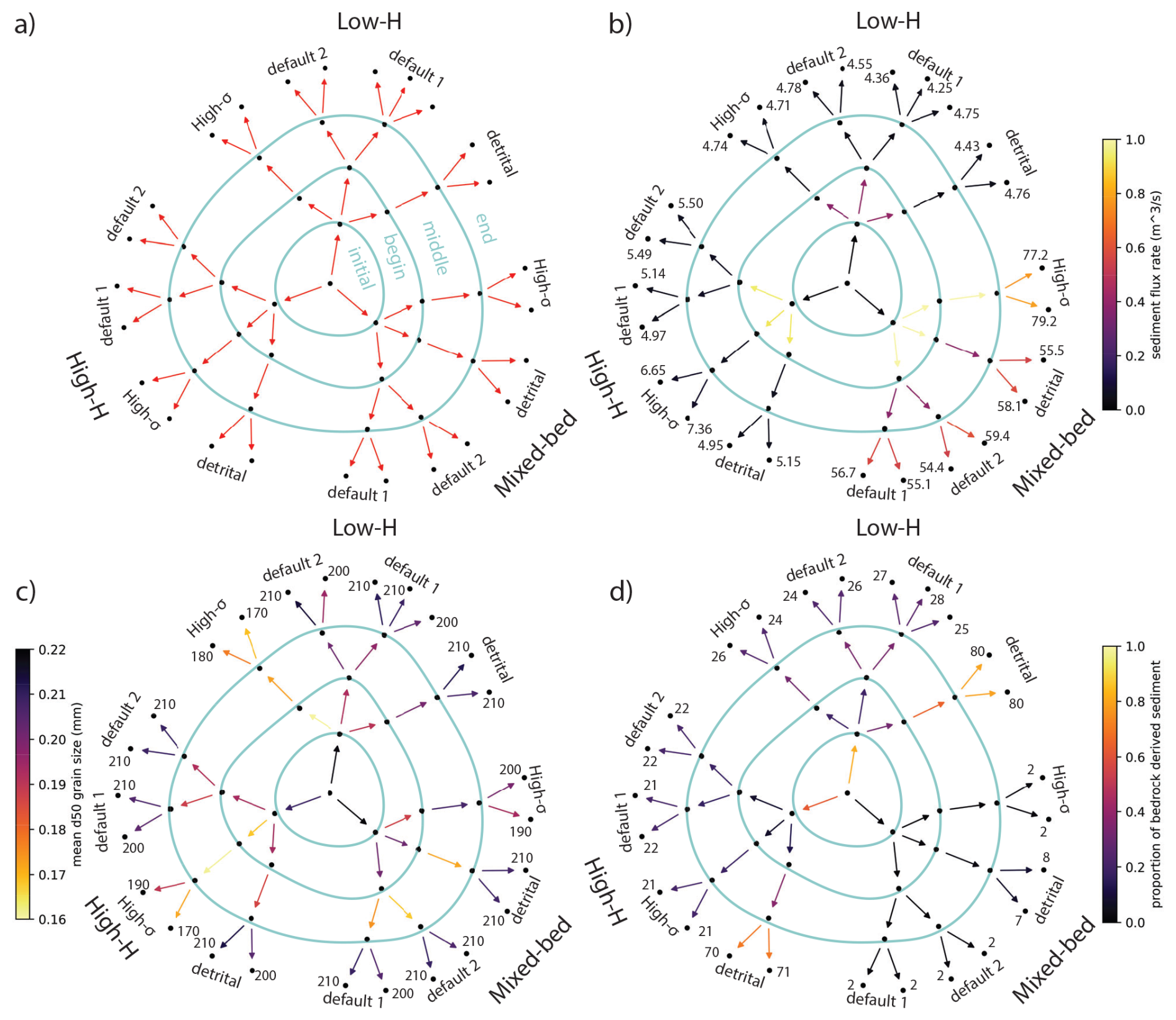
Figure 4 Ensemble structure and summary results including (a) structure of the ensemble trees (b) time-averaged sediment flux rate for each model leg, labeled values in hundredths of m³ s⁻¹. (c) Time-averaged and volume-weighted mean d₅₀ (median grain size) across all outlets for each model leg, labeled values in µm. (d) Volumetric proportion of bedrock-derived sediment for each model leg, labeled values in %. Detrital models show higher values due to the different accounting, see Sect. 3.2.2 and Aitken et al. (2024). Summary data are in Tables A2, A3, and A4.

4 Results

The results for the beginning and middle legs show high and highly variable volumetric discharge (Fig. 4b). These earlier legs represent the period during which the initial condition has not reached a dynamic equilibrium with the seasonal hydrology forcing. For the low-H scenario, the “end” leg model runs show a near-zero net change in sediment thickness and represents a balance between winter gains and summer losses. The high-H runs are similar, but with slightly higher overall discharge and a slight decline in basal sediment thickness. In both these cases, the system is strongly limited by the supply of sediment from erosion. For the mixed bed model, discharge-rates stabilise, but at much higher rates and with a sustained decline in sediment thickness enabled by the much higher availability of sediments. Here, we focus on the result of the end leg.

4.1 low-H scenario

The ensemble result for the low-H scenario (Fig. 5) shows some key features of the sediment system. The sediment discharge rate is low, peaking at ∼ 0.23 m³ s⁻¹. During the melt season a systematic pattern is seen: The early melt season sees mobilisation of basal sediment and an increase in discharge. This early stage shows, in some runs, a distinct peak in grain size, while in others this peak is absent (Fig. 5a). This peak can be attributed to the high transport capacity of high-pressure flow in developing channels combined with the availability of previously-deposited sediment.

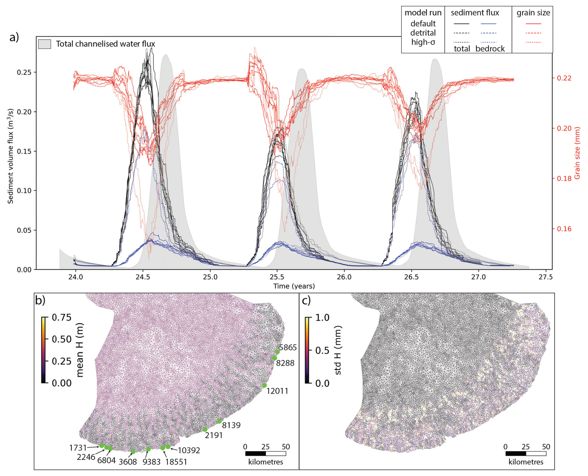
Figure 5 (a) The end-leg results for each member of the low-H ensemble tree showing total sediment flux, sediment flux derived from erosion of bedrock, and volume-weighted average d₅₀. Dashed lines are detrital models, dotted lines high-σ models. The total channelised water flux (from Fig. 3a) is shown for reference (b) ensemble mean sediment thickness and (c) standard deviation in sediment thickness, both at the end of the model run. Labeled green dots indicate the locations of outlet nodes shown in Figs. 10 and 11.

The melt season continues with, at peak discharge, reduced grain size, indicating selective transport of fine grained material from upstream sources. In this scenario the peak sediment discharge occurs well before the peak channelised flow conditions, and the decline is driven by the failure of the supply system. Post peak-discharge, sediment derived from the basal sediment layer reduces, and the grain size recovers to the mean value. By autumn a dominance of bedrock-derived sediment is seen at a low volume, paced by erosion. For this scenario the high-σ mode does not have increased discharge rate, although the sediments are finer. These characteristics indicate that the low-H scenario is strongly supply-limited. The detrital models all have a significantly higher volume of bedrock-derived sediment, which indicates ∼ 2/3 of sediment has experienced at least one cycle through the basal sediment layer.

The remaining basal sediment at the end of the model runs shows a systematic depletion of sediment in channels, extending back ∼ 60 km from the ice margin (Fig. 5b). Variation in the sediment thickness among the ensemble members is low but is highest in the upper reaches of subglacial channels (Fig. 5c).

4.2 high-H scenario

Results for the high-H scenario are fairly similar to the low-H scenario, but with a higher discharge rate and a lower proportion of bedrock-derived sediment (Fig. 6). The peak sediment discharge still precedes the peak channelised flow conditions, indicating a supply limited system. In this case the high-σ mode has a slightly higher discharge rate at peak flow indicating a greater role for sediment transport capacity in controlling supply to the outlet from upstream sources. Correspondingly, the detrital models have approximately half the proportion from bedrock-derived sediment, indicating less recycling through the basal sediment layer than in the low-H scenario.

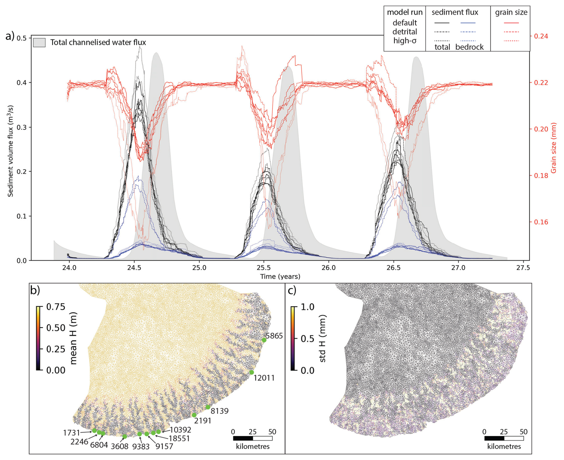
Figure 6 (a) The end-leg results for each member of the high-H ensemble tree showing total sediment flux, sediment flux derived from erosion of bedrock, and volume-weighted average d₅₀. Dashed lines are detrital models, dotted lines high-σ models. The total channelised water flux (from Fig. 3a) is shown for reference (b) ensemble mean sediment thickness and (c) standard deviation in sediment thickness, both at the end of the model run. Labeled green dots indicate the locations of outlet nodes shown in Figs. 10 and 11.

As before, the remaining basal sediment is systematically depleted in channels, extending back ∼ 60 km from the ice margin (Fig. 6b). Variation in the sediment thickness among the ensemble members remains low, and is highest in the upper reaches of subglacial channels (Fig. 6c).

4.3 Mixed-bed scenario

For the mixed-bed scenario, the results are markedly different (Fig. 7). Most notably, the sediment discharge rate is approximately ten times higher than for the low-H and high-H scenarios, and bedrock-derived sediment is a very small proportion. Median grain size still reduces during peak flow, but by much less, and has a less distinct relationship with discharge-rate. In comparison with the low-H and high-H scenarios, the peak sediment discharge is later, and the high-σ mode has markedly higher discharge rate at peak flow. These indicate a more sustained supply and a more significant role for transport capacity in the upstream region controlling supply to the outlet. Despite this, sediment discharge remains far below bulk sediment transport capacity, and supply remains the limiting factor. The detrital models indicate that barely any sediment has been cycled through the basal sediment layer.

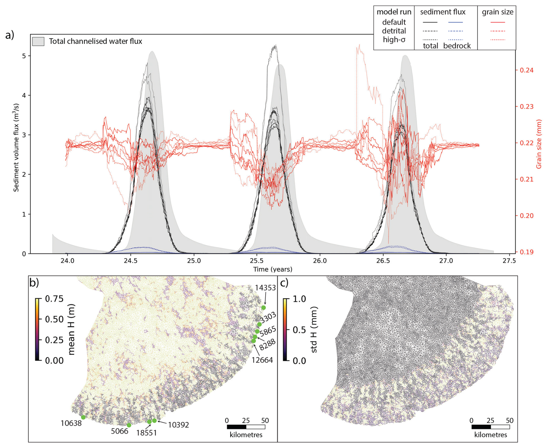
Figure 7 (a) The end-leg results for each member of the mixed-bed ensemble tree showing total sediment flux, sediment flux derived from erosion of bedrock, and volume-weighted average d₅₀. Dashed lines are detrital models, dotted lines high-σ models. The total channelised water flux (from Fig. 3a) is shown for reference (b) ensemble mean sediment thickness and (c) standard deviation in sediment thickness, both at the end of the model run. Labeled green dots indicate the locations of outlet nodes shown in Figs. 10 and 11.

The remaining basal sediment is systematically depleted in channels, reaching zero in many places, but with regions of higher thickness patchily preserved (Fig. 7b). Variation in the sediment thickness among the ensemble members, while still low, is overall higher and more varied than the other scenarios due to the variable initial sediment thickness (Fig. 7c).

5 Discussion

These results highlight some key features of the subglacial sediment system dynamics beneath the FLDIL.

5.1 Seasonal to interannual sediment evolution

The results for the low-H scenario, and to a slightly lesser extent the high-H scenario map out a strongly supply-limited regime where discharge during the melt season is limited by the erosion rate (summed over the year). In these conditions, the seasonal cycle shows a clear zonation. Here we describe the seasonal characteristics of the high-H scenario (Fig. 8).

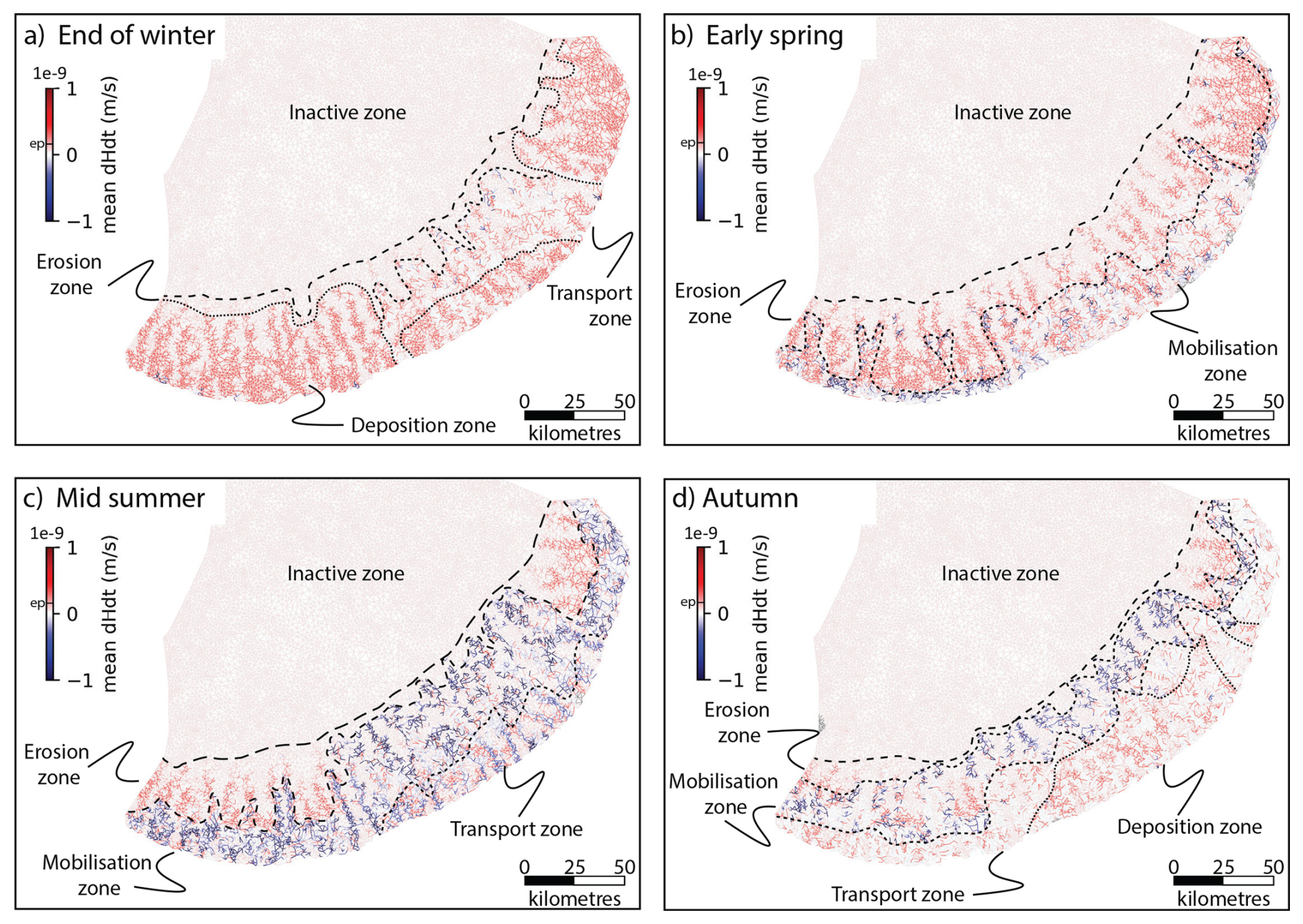
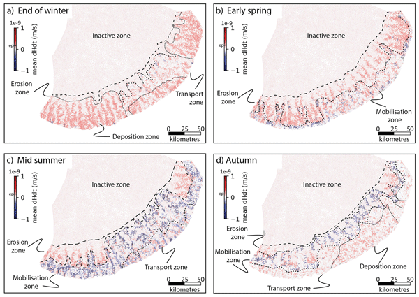
Figure 8 Ensemble mean of $\mathrm{d}H/\mathrm{d}t$ across a melt season for the high-H scenario showing (a) end of winter (b) early spring (onset of melt season) (c) mid-summer (peak hydrology flow) (d) autumn (end of melt season). Interpreted zones of the sedimentary system are shown

At the end of winter (Fig. 8a) the system is dominated by three zones: an inactive zone in the upstream catchment (lacking channels) where $\mathrm{d}H/\mathrm{d}t\approx \mathrm{0}$; a small erosional zone with 0 $<\mathrm{d}H/\mathrm{d}t\le \dot{e}$ ($\dot{e}$ is erosion potential); a transport zone with variable $\mathrm{d}H/\mathrm{d}t$ and a frontal depositional zone with $\mathrm{d}H/\mathrm{d}t>\dot{e}$. Spring (Fig. 8b) sees a different zonation characterised by the development of a mobilisation front. Upstream of the mobilisation front, $\mathrm{d}H/\mathrm{d}t$ is positive, while downstream, channels have negative $\mathrm{d}H/\mathrm{d}t$ as basal sediment is mobilized. Initially, the mobilisation front is close to the ice margin, but then recedes, and by summer is ∼ 20–50 km back from the ice margin (Fig. 8c). This is in line with the processes considered for the deposition of eskers (Núñez Ferreira et al., 2025; Mäkinen, 2003) and murtoos and murtoo-like landforms (Ojala et al., 2019; Mäkinen et al., 2023). A lower transport-zone with both positive and negative $\mathrm{d}H/\mathrm{d}t$ is emergent in summer downstream from the mobilisation front. The back-propagation of the mobilisation front is consistent with the elevation-dependent positive-degree day forcing applied in FLDIL-GlaDS (Hepburn et al., 2024), which, together with ice-thickness exceeding 1 Km, dictates the upstream extent of channelisation. Continuing into autumn, the mobilisation front has reached the upper limit of the channel extents, and has narrowed as basal sediment is depleted downstream. A deposition zone is reformed near the ice margin with positive $\mathrm{d}H/\mathrm{d}t$ (Fig. 8d). The low-H scenario model (Fig. A1) has the following differences attributed to lower sediment availability: the inactive zone sees $\mathrm{d}H/\mathrm{d}t\approx \dot{e}$, mobilisation in the mobilisation front is more localised, and the deposition in front of the mobilisation front is reduced. The mixed-bed scenario (Fig. A2) demonstrates the same behaviours, albeit with increased intensity and spatial variability.

The erosional, mobilisation and depositional zones show corresponding signatures in the grain size of active sediment (Fig. 9). Grain size for freshly eroded sediments is sampled from the population distribution, and erosion-dominated areas tend towards the population mean. In contrast, mobilisation zones show more variation with finer-than-mean grain sizes predominant in Spring and Summer (Figs. 9b and c). In the context of increasing water flow rate, we infer that the drop in mean grain size at the outlets during spring (Figs. 5, 6 and 7) is due to the preferential mobilisation and transport of finer-grained components derived from the basal sediment layer, and that the post-peak return to mean grain size is due to the later predominance of freshly eroded material as upstream supply wanes. This mobilisation and transport bias is strongest in the low-H and high-H scenarios where basal sediment supply sources are located upstream, and less marked in the mixed-bed scenario, where greater volumes of basal sediment are available locally.

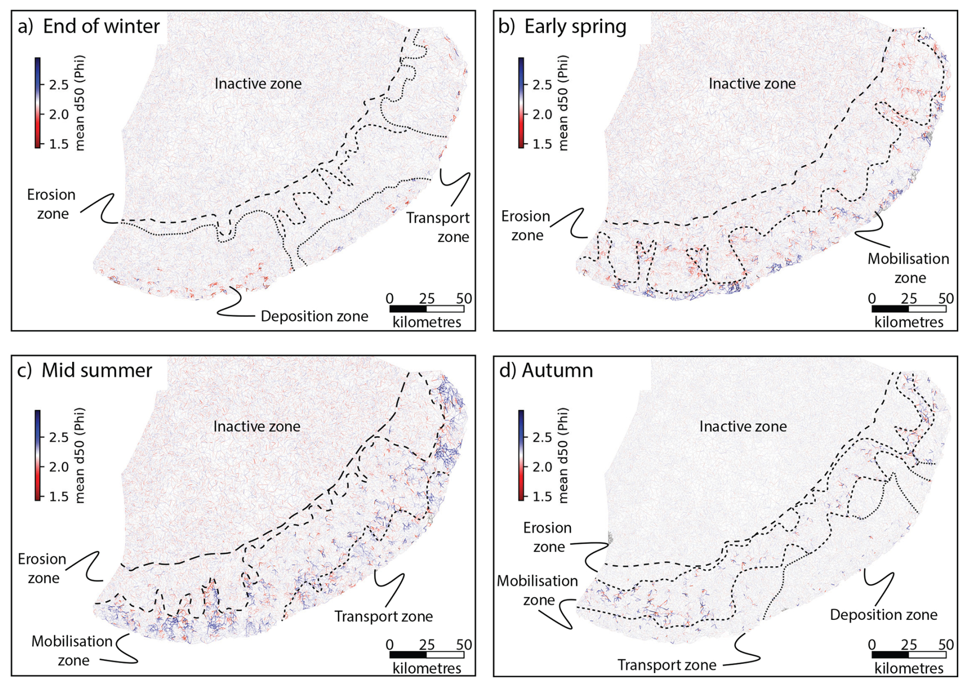
Figure 9 Ensemble mean of active d₅₀, expressed as ϕ, across a melt season for the high-H scenario showing (a) end of winter (b) early spring (onset of melt season) (c) mid-summer (peak hydrology flow) (d) autumn (end of melt season).

Sediment discharge, and sediment properties are tracked at outlet nodes allowing us to analyse a detailed time series of sediment output for specific channels across the model ensemble (Fig. 10). In the low-H and high-H scenarios, we see significant variations in volume output, grain size and detrital character within each melt season. The melt season often begins with a sharp peak in volumetric discharge rate, during which relatively coarse grain sizes (medium-coarse sand) are seen in some cases. Early-season detritus comes from remobilisation of the basal sediment. Through the melt season the volumetric sediment discharge rate typically declines, the grain size reduces to fine or very fine sand, and the proportion of bedrock-derived sediment increases. This systematic behaviour has parallels with the diverse sedimentary settings observed in murtoos in the region, previously linked to variability in water velocity and sediment load (Hovikoski et al., 2023; Ojala et al., 2022). This behaviour is fairly consistent along the ice sheet margin, with no obvious spatial trend in the onset timing or duration of the sediment flux event (Fig. 10). Both the low-H and high-H scenarios indicate a situation where sediments deposited during autumn and winter are remobilised in spring. Discharge is ultimately limited by supply, first as the local basal sediment is depleted, and then by waning supply from upstream sources.

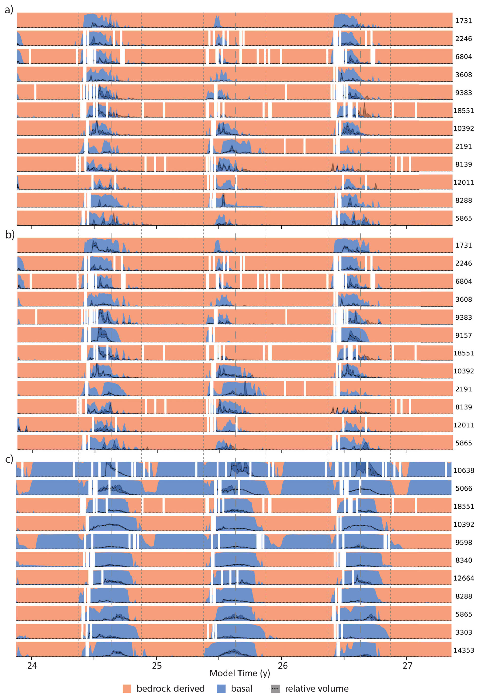
Figure 10 Time-series for major outlet nodes in the “end” period of (a) low-H model ensemble, (b) high-H model ensemble and (c) Mixed-bed model ensemble. For each we exclude the high-σ and detrital branches. The charts show in colours the proportional detrital output derived from bedrock erosion versus basal sediment mobilisation, and the ensemble minimum, median and maximum discharge relative volumes in black. Nodes are ordered west to east, for node locations see Figs. 5, 6 and 7.

The mixed-bed scenario is different, comprising broadly symmetric high-flux events during the melt season, with sediment discharge rate peaking more in line with peak hydrology flow. Grain size in this scenario is more erratic, and the detrital provenance during high flux events is almost entirely derived from the basal sediment layer (Fig. 10). In this scenario the more consistent availability of sediment for some outlets leads to a dichotomy of behaviour in winter: Some outlets show ongoing dominance of basal sediment with fine (but highly variable) grain size (e.g. nodes 9598, 5066) albeit at low discharge rate. In contrast, more sediment-starved outlets are dominated by bedrock-derived sediments with grain size close to the mean (e.g. node 14353) (Fig. 10).

Individual outlets can show significant interannual variability with alternating high- and low-flux seasons, while others show a more consistent series. High-flux seasons have a greater dominance of basal sediment detritus compared to low-flux seasons (Fig. 10). With an erosion-rate limited system, such variations may occur where there is insufficient basal sediment accumulated over winter to sustain concurrent high-flux seasons. Moreover, the hydrology forcing is not consistent year-to-year and channels have variable extents, and sometimes are not formed for one or several years, and then re-established. This hydrologic variability impacts supply as “new” regions of the bed are exposed to sediment mobilising conditions. The more severe interannual variability seen in the low-H and high-H scenarios relative to the mixed-bed scenario points to variable access to the basal sediment layer as the main factor driving interannual variability.

In detrital provenance, (Fig. 11) the discharge in all cases predominantly reflects the local bedrock in the vicinity of the outlet, with relatively little variation. On the basis of these major units, it would be difficult to distinguish between our scenarios, although major changes in the margin location or hydrological structure (for example, focusing of flow towards the north or south) could be observed. In some cases, minor units are seen only during the melt season, such as the volcanic units seen at nodes 6804, 2246 and 1731 (for locations, see Fig. 5). These units, if observed in detritus, could act as markers of the extent and location of channelized flow.

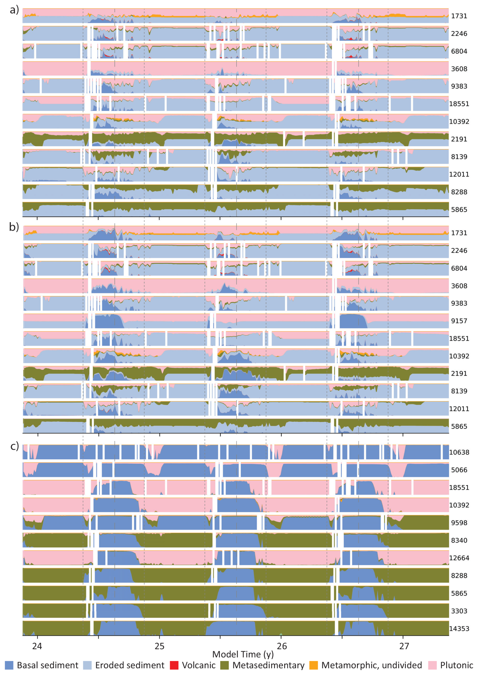
Figure 11 Time-series of detrital output for major outlet nodes in the detrital branch models showing (a) low-H, (b) high-H, and (c) mixed-bed. Nodes for each model are ordered from west to east (for locations see Figs. 5, 6 and 7). Colours here map to Fig. 1b. Map units not listed here did not yield any detritus

5.2 Outcomes

This work set out to address three research questions, for which we may now review the progress made:

1. Can the sub- to pro-glacial sediment dynamics of the FLDIL be well represented in a hydrology-forced sediment system model?

   The sediment system was adequately represented for timescales of weeks to several years, yielding internally consistent results across ensemble members in each scenario and between the low-H and high-H scenarios. The seasonal behaviours of the sediment system were particularly well resolved and generate variations in sediment yield and grain size characteristics that compare well to sedimentary observations from both murtoos and eskers (Hovikoski et al., 2023; Ojala et al., 2022; Mäkinen, 2003). The interannual record is more limited due to the length of the model run, however, the observed variations in sediment characteristics are consistent with “flow switching” under varying hydrological forcing as a driver of the geomorphological complexity seen in nature (Palmu et al., 2021; GTK Finland, 2025c).

   Both longer-term and shorter-term impacts on sediment transport may be important (Delaney et al., 2026) and are not included in this modelling study. In particular, diurnal melt cycles were not included in the GlaDS forcing. Prior modelling studies show that including diurnal melt cycles can increase net sediment transport, in line with peak daily flow conditions (Aitken, 2024). Diurnal cyclicity could further impact the onset timing and duration of seasonal events and the areal extent of the bed exposed to active transport processes. In this case, net sediment transport over annual timescales would likely be similar due to the model scenarios being strongly supply limited. For this model study all scenarios reach a consistent discharge rate within 10 years. Supra-decadal influences may include longer-term drivers of sediment supply, including retreat and advance of the margin location and re-routing of subglacial hydrology due to changes in ice dynamics. Compared to the static ice margin here, a margin evolution including such variations would be expected to access a more extensive area of the bed over time and sustain sediment supply for longer.

   A limitation of the GlaDS-GraphSSeT approach applied is that the sediment evolution does not feed back into the hydrology conditions, although in nature the evolving subglacial sediment distribution may be an important factor for controlling hydrology, for example the filling of channels during esker formation affecting area and shape (Hewitt and Creyts, 2019), and interactions linked to transitions between distributed and channelised flow (Swift et al., 2021). In this study we have very low rates of sediment mobilisation and deposition relative to the size of the channels, and the effect of these small volumes on channel geometry are negligible over the model duration. Ice marginal landforms may start as subaqueous fans and, if sediment delivery is sufficient, may grow to form Hjulström-type or Gilbert-types of ice contact delta depending on water depth (Hovikoski et al., 2026), these deltas potentially impacting the upstream hydrology. At the outlet, we assume for this study that the depositional system can accept all sediment without building up any constriction; again the volumes are very small over the model duration. Although the very small sediment volumes involved over 10 years would not have any significant impact on the hydrological system, their accumulation over long periods may lead to systematic long-term changes that this study does not resolve.

2. Can the sediment system model explain geological observables, including subglacial sediment thickness, and the characteristics and spatial distribution of ice-marginal deposits?

   The sediment system model yields geologically realistic outputs that are consistent with the formation of the observed subglacial and proglacial landforms. These include the preservation of the preglacial landscape in the ice sheet interior, with a sediment-depleted submarginal-zone, and implied extensive ice-marginal deposits. The outlet detritus is dominated by sand, without marked variations in volume along the margin, but with spaced outlets of major channels giving localised depocentres. These depocentres and the gaps between them, bear similarity to the patterns of glaciofluvial landforms (GTK Finland, 2025c) and deposits observed in the Salpausselkä II (Fig. 1).

   For grain size, we resolve a systematic annual signal of a coarse spring onset, fining upwards into summer indicating an influx of finer-grained transported material. In a proglacial lake setting such as Salpausselkä II this would likely be represented by an ice-contact delta (Lunkka, 2023) and clastic varves composed of fine-grained silt and clay deposited at the margin and in a proglacial basin in front of the retreating glacier (Zolitschka et al., 2015). This coarser-to-finer grain size variation is accompanied by a change in detritus from reworked basal sediment grading to bedrock-derived sediment. In some cases this change is marked by lithologies that are not seen during low-flux periods, and these could be viable targets for detrital provenance analysis.

   With a model run of 10 years' duration the pattern of sediment depletion, preservation and deposition is effectively represented with clear similarity to the observed distribution. The model resolves an intensive sediment depletion zone for ∼ 50 km behind the ice margin, and behind this, preservation of pre-existing sediment. These are consistent with the pattern seen in sediment thickness data (Fig. 1) and with the interpreted glacial evolution, which is very dynamic and fast-changing (Lunkka et al., 2021; Ojala et al., 2019, 2022; Mäkinen et al., 2023). Some contrasts exist: for example we do not resolve linear regions of thinner sediment extending for ∼ 150 km. These likely formed as a result of a focused channel network at some stage. FLDIL-GlaDS model testing shows such long channels are difficult to generate with reasonable forcing, and are not consistent with the margin location advanced to the Salpausselkä II (Hepburn et al., 2024). A model incorporating time-trangressive ice-margin evolution would potentially be able to resolve some of these features.

   Although in-channel fluvial deposition is resolved, the model does not yield eskers because virtually all the sediment deposited during autumn and winter is remobilised in the next melt season (Fig.8). Coarse-sand and gravel grain size is a key feature of esker formation during channel expansion in the early melt season (Mäkinen, 2003) and these coarse-grained deposits are much less susceptible to remobilisation. GraphSSeT does not consider englacial processes and subglacial fluvial transport capacity for gravel grain sizes and larger is limited in the modeled scenarios, so the coarse-grained sediment needed to build the esker core is not represented.

   The Salpausselkä II comprises the major sedimentary deposit for the FLDIL configuration of the Younger Dryas ice sheet. For Salpausselkä II we estimate the volume of sand at ∼ 30 km³ (see Appendix A). Geological data suggest the Salpausselkä II formed within an estimated timeframe of 500 to 1000 years (Lunkka et al., 2021; Joakim Donner, 2010). This implies an average sediment discharge rate of ∼ 0.95 to 1.90 m³ s⁻¹, although formation was likely in discrete episodes of more rapid deposition, and with imperfect preservation (Lunkka, 2023; Palmu et al., 2021). To build up the Salpausselkä II volume at the rates of discharge in our models for the low-H and high-H scenarios, would take ∼ 20 and ∼ 16 cal. ka respectively – such rates of discharge are clearly insufficient. A model run at transport capacity (i.e. without any limits imposed on sediment supply) has discharge rates of ∼ 60 m³ s⁻¹, requiring just 15 to 20 years to supply the volume for the Salpausselkä II. The mixed-bed scenario needs ∼ 1500 years to supply the required volume for Salpausselkä II and is the most plausible of our series of models. The implication is that formation of the Salpausselkä II was critically controlled by the limited availability of sediment and involved the re-mobilisation of a sediment cover not dissimilar to today's, but likely more extensive in the now depleted sub-marginal zone.

3. Can the comparison of geological observables with the sediment model outcomes help to better constrain ice sheet and subglacial hydrology system evolutions?

   The geomorphology, stratigraphy, grain size and detrital signatures of glacial sediments are commonly used as diagnostic tools for reconstructing glacial systems (Licht and Hemming, 2017; Ojala et al., 2019; Lunkka, 2023; Lunkka et al., 2021). As well as tracking volumes and thicknesses, the model results resolve two significant features that can be used to constrain interpretations. First is the systemic co-variation of fining-up grain size and decreasing maturity of the detrital provenance during high-flux events, giving criteria for identification of these events in sediment cores. The second is the identification of “indicator” detrital units (see; Aitken and Urosevic, 2021) found only in the fresh detritus during high flux events. These may prove good targets for detrital fingerprinting as they are spatially discrete, geologically distinct and clearly tied to the subglacial hydrology conditions.

5.3 Future directions

Future work may look to refine the approach and resolve some of the deficits identified in this work.

The choice of the initial conditions was very significant for model evolution, in particular, the thickness and distribution of pre-existing sediment cover was in this case the critical factor controlling sediment supply. For accurate volume calculations, this initial condition must be known well, which is challenging for both modern subglacial systems and past examples. A strong control on initial conditions requires robust knowledge of the ice sheet and its subglacial hydrology, constrained by the subglacial environment and its past history and the characteristics of glacial deposits. We show for the FLDIL, where these factors are reasonably well known, the forward-model approach allows us to reject unsuitable initial conditions. For less well constrained examples, data-constrained model ensembles may be sought using inverse-methods that couple geological and geophysical data with the model outputs.

The realistic, but relatively narrow grain size distribution used here (Vorren, 1977) focuses this study on sands, consistent with the majority (∼ 80 %) of sediment observed in the region, but does not allow to analyse the origins of the extensive gravel deposits. In particular, we do not test if they are subject to significant fluvial transport, and over what timescales this might occur.

Interannual variations were detected for many outlets, however, the 10-year model run, after the “burn in” period, did not allow to resolve this over multiple cycles. A longer model run could allow this to be more fully tested, and to investigate more fully the interaction between variable hydrology forcing and evolving sediment availability.

Eskers and sediment-free zones extending hundreds of kilometers beneath the ice are not a feature of our model. Such features are inconsistent with a model domain fixed at the Salpausselkä II, and would instead require a time-transgressive margin evolution (see; Mäkinen, 2003) over longer time periods than considered here. Additionally, longer-term transport of coarse-grained sediment by englacial processes are likely important in order to provide a consistent source of coarse-grained sediment to the ice margin (Mäkinen, 2003).

6 Conclusions

This work applied the GraphSSeT sediment system model with forcing from a recent GlaDS model of the FLDIL for three different scenarios. Our modelling resolves, for these scenarios, a realistic pattern of subglacial sediment depletion, preservation, and deposition that matches the sediment thickness patterns observed in the subglacial and proglacial landscape of the FLDIL. The model robustly predicts seasonal cyclicity in the sediment supply, transport and deposition system with characteristics that are clearly linked to the hydrological forcing. The sediment characteristics predicted by the model, while not designed to explain specific features, have volumes, grain size distributions, and seasonal evolutions that match observations from glaciofluvial landforms such as murtoos and eskers (Hovikoski et al., 2023; Mäkinen, 2003; Ojala et al., 2021). The model is able to explain the supply of sediment for Salpausselkä II with a supply-limited system involving a distributed sediment cover similar to but likely more extensive than today's, at the same time excluding erosion-rate limited and transport-capacity limited models. The model has allowed a stronger comparison between numerical models of the past ice-sheet and hydrology system, and key observations in the sedimentary record, strengthening the links already made (Hepburn et al., 2024; Ojala et al., 2022), and lending increased confidence to interpretations of the FLDIL in the Younger Dryas stadial. Looking to the modern Earth, models such as this can be used to constrain sediment-based interpretations of glacial conditions in Antarctica and Greenland and the associated impacts on landscapes and ecological and ocean systems now and into the future.

Appendix A

Calculation of the volume of the Salpausselkä II, and timeframes for its deposition, used data sets freely available from the GTK Finland web-server (GTK Finland, 2025c, d, a) and was generated with the following process.

Ice marginal deposits (from GTK Finland, 2025c) were clipped within the model domain. For each feature, the mean sediment thickness (from GTK Finland, 2025d) was calculated using zonal statistics. Multiplying this by feature area yields the estimated volume of the Salpausselkä II (within the model domain) of 38.5 km³.

For the ice-marginal deposit features a spatial join was performed with the sand and gravel resources data (from GTK Finland, 2025a). Across the joined dataset the relative proportions of hiekka (sand), sora (gravel), and murskavatta (larger rocks) were calculated, yielding 78.0 % sand, 20.2 % gravel and 1.8 % larger rocks. Our model does not capture gravel transport so we assess the total sand volume in Salpausselkä II as 78 % of 38.5, i.e. 30 km³.

From the total sediment yield of our model runs we can calculate the time required to supply this sand volume (Table A1). We sum total sediment yield from “beginning”, “middle” and “end” legs to yield the residual volume needed to reach the total sand volume in the Salpausselkä II. The time required to reach the target volume is estimated by extrapolating the sediment discharge rate from the “end” model leg until the required volume is reached.

Table A1 Total volume discharge and estimate of time required to reach the total sand volume in Salpausselkä II. The infinite-till model assumes that basal sediment is always available and represents a purely transport-capacity limited scenario.

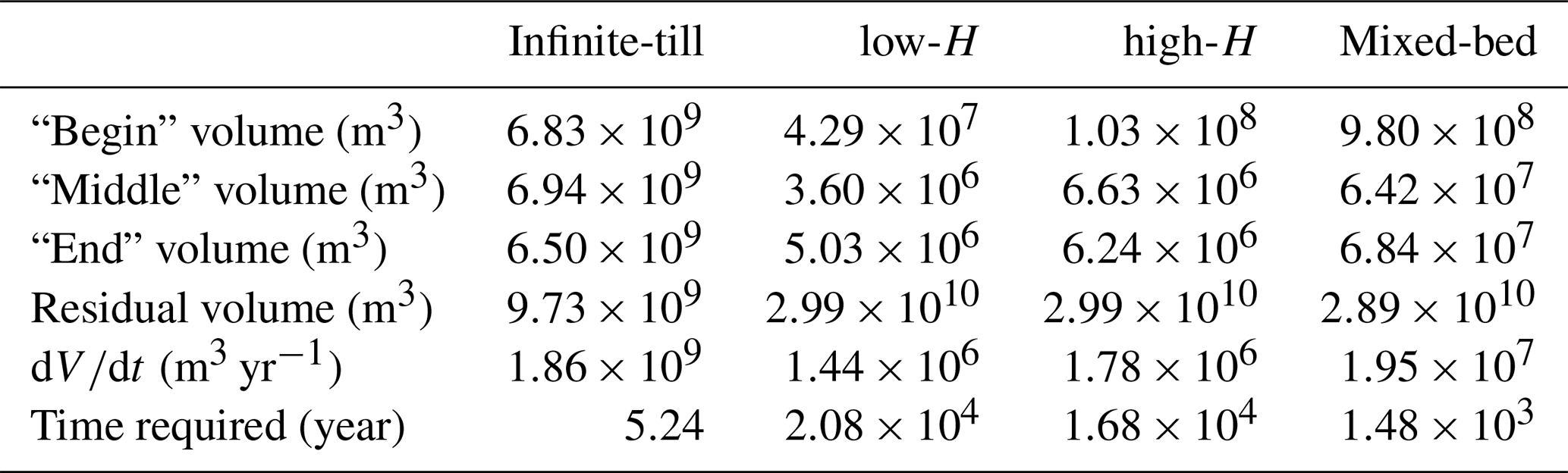
Table A2 List of model runs and key output parameters for the low-H scenario model ensemble.

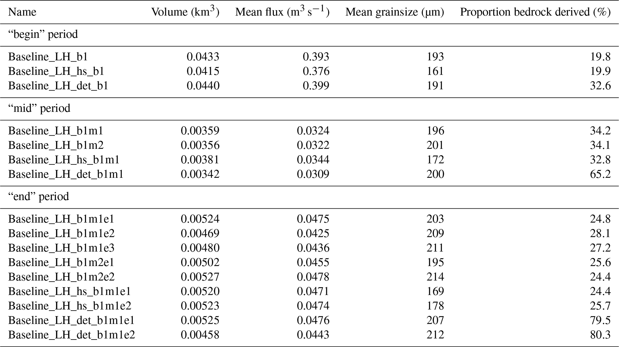
Table A3 List of model runs and key output parameters for the high-H scenario model ensemble.

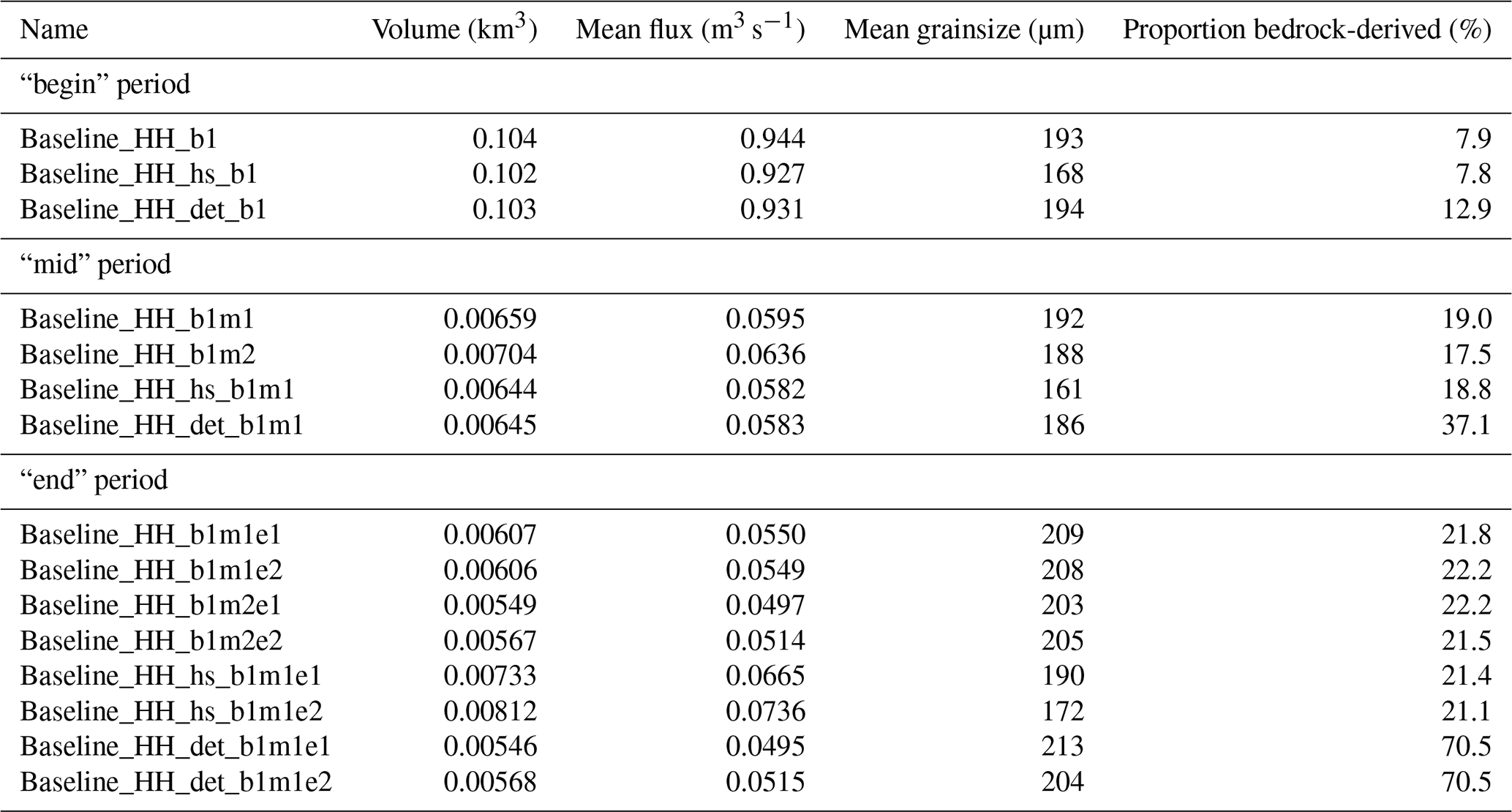
Table A4 List of model runs and key output parameters for the Mixed-Bed scenario model ensemble.

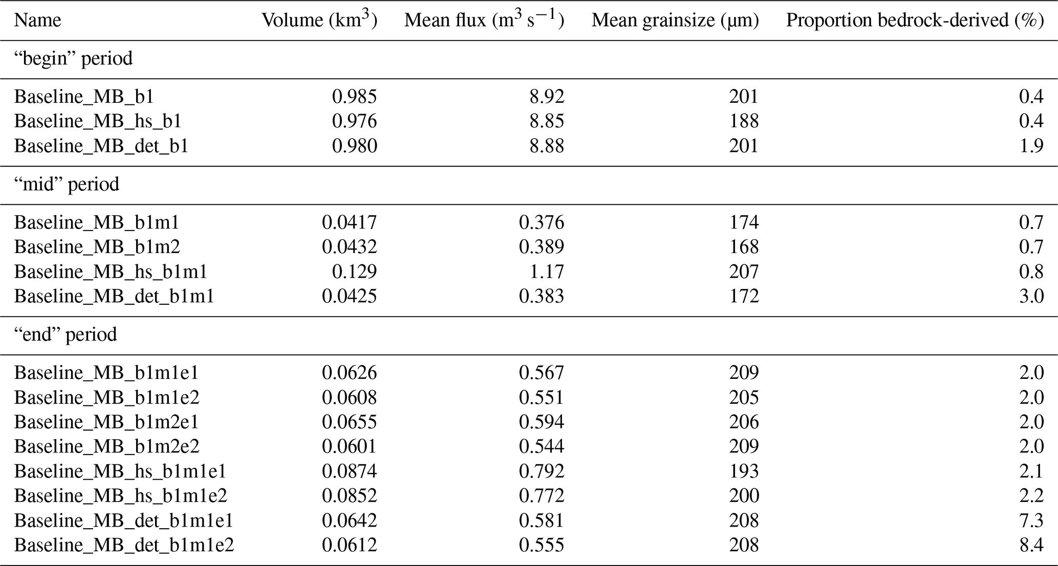
Table A5 List of model runs and key output parameters for the infinite till model run. In infinite till mode GraphSSeT assumes basal sediment is always available and therefore represents a purely transport limited case. Grain size is fixed at the mean of the population distribution.

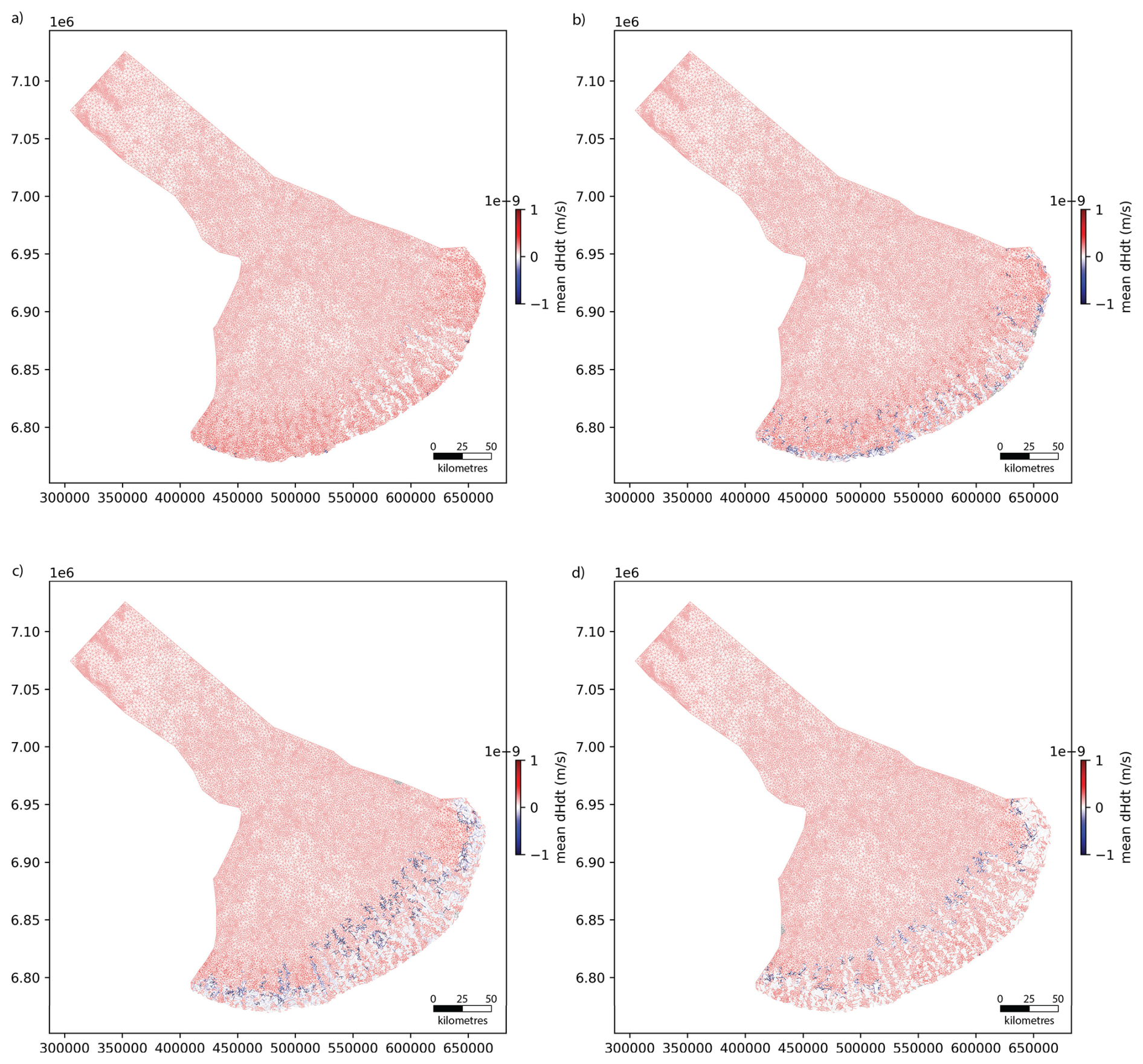
Figure A1 Ensemble mean of $\mathrm{d}H/\mathrm{d}t$ across a melt season for the low-H scenario showing (a) end of winter (b) early spring (onset of melt season) (c) mid-summer (peak hydrology flow) (d) autumn (end of melt season).

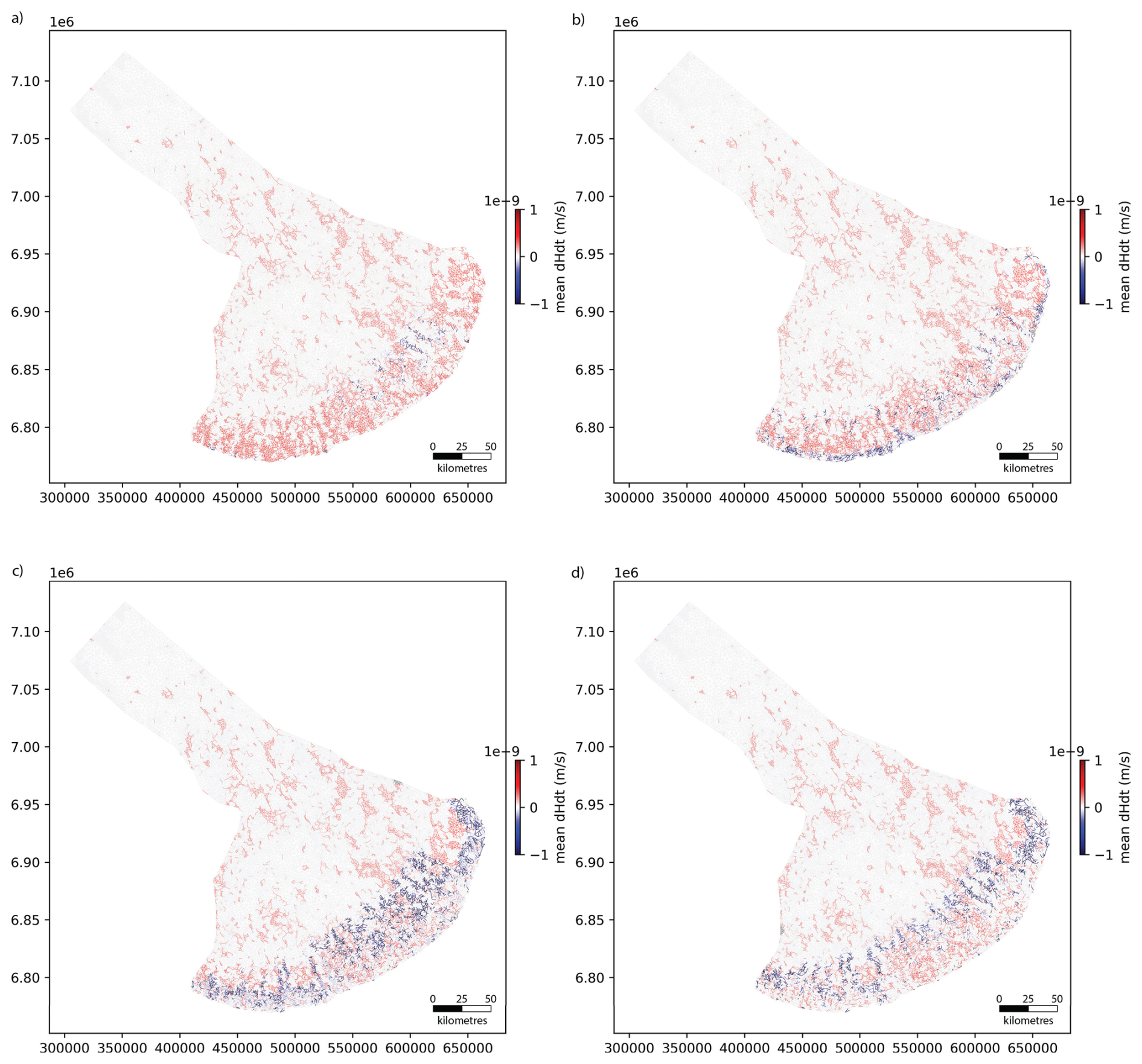
Figure A2 Ensemble mean of $\mathrm{d}H/\mathrm{d}t$ across a melt season for the mixed-bed scenario showing (a) end of winter (b) early spring (onset of melt season) (c) mid-summer (peak hydrology flow) (d) autumn (end of melt season).