Sensitivity of the Bootstrap sea ice concentration algorithm to surface parameters in the Antarctic marginal ice zone using passive microwave retrievals

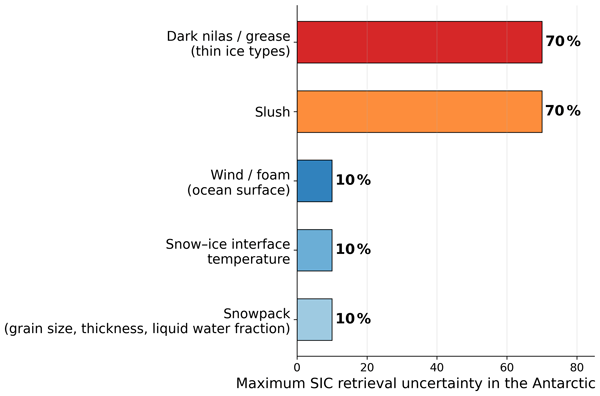
Changes in sea ice concentration (SIC) and derived sea ice extent have been monitored using microwave radiometers since the late 1970s, providing information about the polar response to climate change, making SIC an invaluable variable for numerical models. Antarctic sea ice has experienced an unprecedented decline in the past decade (2016–2025). In the highly dynamic Marginal Ice Zone (MIZ), the region in between the pack ice and the open ocean, physical properties undergo intense variability, which may impact the accuracy of the SIC products retrieved from brightness temperature measurements. For the purpose of this study, the MIZ is defined as the area with SIC between 15 % and 80 %. We simulate the variations of brightness temperature due to changes in the physical parameters describing the sea ice, the snow, and the ocean with the Snow Microwave Radiative Transfer Model (SMRT) and the Passive and Active Reference Microwave to Infrared Ocean model (PARMIO) for a range of prescribed SIC. We then apply the core of the Bootstrap SIC algorithm on the simulated brightness temperatures and compare the retrieved SIC with the prescribed true SIC, yielding the SIC retrieval uncertainty. This allows us to assess the impact of changes on the SIC retrieval by means of numerical radiative transfer simulations. The work identifies the key parameters leading to high uncertainty in the retrieval. In the snowpack, the liquid water fraction, snow grain size, thickness, and snow–ice interface temperature each cause SIC uncertainties within the 5 % range, with some parameters reaching up to 10 % depending on the season. However, the most dominant uncertainty in the cold season comes from the presence of thin ice types like dark nilas and grease, characterised by high salinity or liquid water fraction, which induce uncertainties of up to 70 %. This uncertainty is comparable to that caused by slush, which can be found in the MIZ all year round. Ocean surface impacted by the high-wind conditions affects both warm and cold seasons and gives rise to uncertainties of up to 10 % on the lower SIC MIZ boundary. However, other parameters that were expected to modify the SIC results, such as the temperature and salinity in the snowpack overlying the first-year ice, showed a negligible impact in the tested range. We found that the core of the Bootstrap algorithm is largely robust to the variations in the snowpack properties. In contrast, the presence of thin ice types and slush and ocean surface affected by high wind speeds in the grid cell are the variables leading to the greatest uncertainties, suggesting they are the primary targets to achieve more accurate SIC retrievals in the MIZ.

1 Introduction

The Marginal Ice Zone (MIZ) – the region that separates the pack ice from the open ocean – is a highly dynamic environment featuring continuous interaction between the ocean and the atmosphere (Morison and McPhee, 2001; Bennetts et al., 2022; Dumont, 2022; Vichi, 2022). These exchanges have ongoing impact on the physical structure of the sea ice and the characteristics of the snowpack on top of it (Massom et al., 2001). Understanding the drivers of the interactions between the sea ice, the ocean, and the atmosphere is essential to explain the factors that contribute to the decline of sea ice extent, including the unprecedented minimum recorded in the Southern Ocean in summer 2023 (Maksym, 2019; Purich and Doddridge, 2023).

The sea ice concentration (SIC) is the fraction of a known ocean area covered by sea ice (Comiso, 2009; Lavergne et al., 2022). Satellite observations are exploited to retrieve SIC through the brightness temperature (T_B) measured by microwave radiometers in frequencies between 6 and 89 GHz, in the vertical (V) and horizontal (H) polarisation (Cavalieri et al., 1984; Swift et al., 1985; Comiso, 1995). Passive microwave (PM) observations are valuable to study snow metamorphisms, changes in the physical properties of sea ice, or the ocean surface because they provide synoptic and continuous observations that are independent on daylight conditions and largely unaffected by cloud coverage, not available otherwise (Parkinson and Cavalieri, 2008; Comiso et al., 2017a, b).

The combination of brightness temperature observations at different frequencies or polarisations constitutes a signature that differs across surface types (Comiso et al., 1997). In the case of sea ice, it is dependent on the physical properties of the ice and snow cover. In the Antarctic, not only the sea ice changes significantly with time and region, but also the snow on top of it. Snow on sea ice undergoes high variability due to redistribution caused by frequent strong winds, seawater flooding, salinity variations and snow ice formation from sea ice overload, and daily melt-thaw cycles. All these processes largely affect the surface and internal properties of the snow, which in turn leads to wide variations in T_B (Macelloni et al., 2001; Massom et al., 2001; Mathew et al., 2009; Willmes et al., 2014; Wang et al., 2024). In addition, the retreat of sea ice means an increased proportion of the marginal ice zone (Strong and Rigor, 2013) and enhanced wave-ice interaction (Bennetts et al., 2022). There is, therefore, an emerging necessity to have more accurate SIC retrieval at low concentration (Kern et al., 2022) and a better understanding of the passive microwave brightness temperature variability in the MIZ. The risk is, otherwise, to mask wave-ice processes with SIC uncertainties (Nose et al., 2020). Understanding the impact of the varying properties of snow and ice on the retrieved SIC remains a challenge in the Southern Ocean (Vichi, 2022), especially in the MIZ (Worby, 2004), where the increasing contribution of the ocean (Meissner and Wentz, 2002) to the grid cell signal (due to low SIC), introduces further T_B variations alongside the processes of formation and development of sea ice (Matsumura and Ohshima, 2015; Paul et al., 2021).

This study evaluates uncertainties in the SIC retrieval induced by changes in the physical properties of the snow–sea ice–ocean system. Building on previous investigations (Andersen et al., 2006; Tonboe et al., 2011; Willmes et al., 2014; Tonboe et al., 2022), we quantify the non-unique relationship between T_B and sea ice concentration, arising from the different snow and ice characteristics that produce different microwave signatures at the same ice concentration. To understand the drivers of the PM signature, we perform a sensitivity analysis on these properties through a radiative transfer computation by perturbing each physical parameter independently to explicitly quantify the brightness temperature variability across the full SIC range, with particular focus on the marginal ice zone. We use a combination of two state-of-the-art radiative transfer models to simulate the passive microwave observations of the ocean and sea ice components of the MIZ, which are then combined to obtain a mixed grid cell for both the warm and cold seasons. Sea ice is modelled with the Snow Microwave Radiative Transfer Model (SMRT) (Picard et al., 2018), which computes the radiative transfer in a multilayer snowpack, sea ice, underlying ocean and overlying atmosphere. The ocean is modelled with the Passive and Active Reference Microwave to Infrared Ocean (PARMIO) (Dinnat et al., 2023), used to simulate the emissivity of the ocean, overlaid by the atmosphere. By employing SMRT and PARMIO together, to have modularity and flexibility, we perform a sensitivity analysis of the physical properties of the sea ice, ocean and atmospheric components, sampling a broad range of parameters drawn from the literature to represent the circumpolar variability across two seasons. This includes the snowpack parameters of first-year sea ice, as well as atmospheric parameters over the open ocean, including wind speed, and ERA5-informed atmospheric profiles. In addition, we simulate the brightness temperature signatures of ice types characteristic of the MIZ, including dark nilas, grease ice and slush and their mixing with the first-year sea ice.

We then employ a technique based on the Bootstrap algorithm (Comiso, 1986) to compute the SIC for each sensitivity experiment and compare the results against a reference simulation, treated as the true SIC. Thus, we evaluate the uncertainty introduced by each parameter on the retrieved SIC as the variability around a reference. The area of interest is the low-concentration MIZ, whose boundaries are considered between 15 % and 80 % SIC (Strong and Rigor, 2013), and where the ocean contributes strongly to the mixed-grid cell signal, leading to a signature that differs substantially from that of the consolidated ice pack. Accordingly, we chose to work with the Bootstrap algorithm in frequency mode (BF algorithm) as it performs comparatively better in regions dominated by open water (Andersen et al., 2007; Ivanova et al., 2015).

The paper is structured as follows: Sect. 2 provides the background on passive microwave SIC retrieval. Section 3.1, 3.1.2, 3.2 and 3.3 describe the cryospheric, ocean and atmospheric components, for the mixed grid cell simulation. The observations used to support the forward modelling approach are presented in Sect. 3.4. The model parametrisation is adopted to analyse the variability of the snow-covered sea ice signature in Sect. 3.5 and the algorithm for the sensitivity analysis of the ocean and sea ice parameters on SIC simulations is in Sect. 3.6. Results are presented in Sect. 4, first addressing the simulated observational variability (Sect. 4.1) and then the SIC sensitivity analysis (Sect. 4.2). Finally, Sect. 5 discusses the findings, their limitations, and future perspectives.

2 Background

Many SIC retrieval algorithms rely on the contrast of microwave emission between the sea ice (high emission) and ocean (low emission) (Comiso et al., 1984; Steffen and Schweiger, 1991; Comiso, 1995; Markus and Cavalieri, 2000). They assume linear mixing, which means that the T_B observed over a mixed grid cell is the sum of the brightness temperature over its ocean and sea ice components weighted by their respective proportions (Comiso and Sullivan, 1986; Comiso, 2012; Ivanova et al., 2015; Comiso et al., 2017b; Meier and Stewart, 2020). These methods usually evaluate the linear relationship in a two-dimensional space defined by two microwave channels, a channel being the T_B at a given frequency and polarisation, hereafter denoted by its frequency in GHz followed by its polarisation (e.g., 19 V). The most commonly used in sea ice studies are the 37 V–37 H or the 19–37 V, with the latter combination preferred in the Antarctic MIZ, and used in the BF algorithm (Comiso and Sullivan, 1986; Ivanova et al., 2015; Meier and Stewart, 2020). The BF algorithm (Comiso, 1986) exploits the following relation:

$$\begin{array}{}\text{(1)}& T_{\mathrm{B}}\left(P\right)=T_{\mathrm{SI}}{C}_{\mathrm{I}}+T_{\mathrm{OO}}(\mathrm{1}-C_{\mathrm{I}})\end{array}$$

where C_I is the sea ice concentration, T_B is the observed brightness temperature, T_SI and T_OO are the brightness temperatures of 100 % sea ice and 100 % ocean respectively, which in the 19–37 V channel space tend to appear in two different clusters (Swift et al., 1985; Comiso, 1995), and define the algorithm tie points. Through the sea ice tie point (T_SI), passes a line with a slope determined by linear regression of the 100 % SIC cluster. Variations along this line result from modifications of sea ice and snowpack properties. Data points distributed around the ocean tie points represent 100 % open water with different surface states. The Bootstrap algorithm, among others, adjusts the tie points and the 100 % SIC line on a daily basis to account for the variability that depends on season and meteorological conditions (Comiso, 2013). The T_B signatures in between these tie points belong to grid cells with different SIC values (Eq. 1). However, different snow and ice characteristics lead to different microwave signatures also when considered in the same concentration, introducing a non-unique relationship between T_B and SIC.

The SIC retrievals are sensitive to variability in the atmosphere and surface emissivity, with the degree of sensitivity depending on the channels employed by the algorithm. One definition of the total uncertainty on SIC retrievals is through two components: the algorithm uncertainty, which includes sensor noise and the residual geophysical variability of the ocean, sea ice and atmosphere, which is the focus of this study, and the smearing uncertainty, arising from the mismatch between satellite footprints and the target grid (Tonboe et al., 2016; Lavergne et al., 2019), which we do not address in this work. Among the algorithm uncertainty components, a first source arises from the surface. The assumption that different ice types lead to distinct brightness temperatures means that ice differing in snow depth, snowpack layering, snow wetness, salinity and temperature yields retrieved SIC values scattered around the true SIC (Tonboe et al., 2011, 2022; Willmes et al., 2014). This physical variability of the surface introduces a retrieval scatter even under fully consolidated ice conditions (Kern et al., 2019), leading unavoidably to uncertainty in the retrieved SIC. A mixture of ice types leads to a non-straight 100 % SIC ice line, which, if accounted for, can yield reduced SIC variability (Lavergne et al., 2019; Tonboe et al., 2022), especially when using the BF algorithm. In the Antarctic, surface signature scatter is more pronounced compared to the Arctic, due to snow metamorphism following daily thaw-freeze cycles (Willmes et al., 2014; Kern et al., 2022) and sea ice flooding leading to wet snow ice formation at the interface between the sea ice and the snowpack. In the cold season, the formation of young nilas and grey-white thin ice (<0.2 m) (Ivanova et al., 2015) is characterised by a TB signature intermediate between open ocean and consolidated sea ice, which evolves very rapidly, particularly in the first few hours following formation due to rapid changes in temperature and thickness and brine volume drainage (Kwok et al., 2007; Naoki et al., 2008). This leads to SIC underestimation across all algorithms (Tonboe et al., 2022) and can affect extended surface areas across multiple grid cells, or sub-grid scale at the opening of leads, producing different signatures even between two consecutive satellite passages. A second source of uncertainty arises from atmospheric variability, mostly over the open ocean. Weather effects, including wind speed, cloud liquid water and water vapour, cause the ocean brightness temperatures to scatter around the open water tie point, introducing random noise in the retrieval (Lavergne et al., 2019), with larger impact at lower SIC compared to fully consolidated ice (Andersen et al., 2006; Lavergne et al., 2019; Kern et al., 2019). This noise can be partially reduced through numerical weather predictions, radiative transfer models applied regionally (Andersen et al., 2006; Kern, 2004), weather filters (Cavalieri et al., 1995) and atmospheric correction. However, these corrections have limitations: when atmospheric conditions are moderate and cloud liquid water or water vapour content is low, weather filters can erroneously suppress the sea ice signal, setting SIC to 0 % particularly near the ice edge (Andersen et al., 2006; Spreen et al., 2008; Lavergne et al., 2019). These sources of uncertainty manifest differently depending on concentration, regime and season. The variability increases from winter to early summer (Willmes et al., 2014). In early summer, most SIC products show overestimation at higher concentrations and underestimation in the marginal ice zone (Kern et al., 2019). Generally, most products tend to underestimate SIC when concentrations are below 50 % (Kern et al., 2019). Such over- and underestimation (Ivanova et al., 2014) introduces errors in informing climate models (Niederdrenk and Notz, 2018), motivating continued efforts in algorithm development, intercomparison (Ivanova et al., 2015) and validation against both in-situ and satellite observations (Andersen et al., 2007; Tonboe et al., 2016; Kern et al., 2019, 2022; Lavergne et al., 2019), including the capability to transition consistently between the summer and winter seasons. The underestimation is particularly pronounced in the MIZ, where the presence of thin and mixed ice types makes SIC retrieval especially challenging.

3 Methods and Data

3.1 Cryospheric brightness temperature simulation

We employ the SMRT model (Picard et al., 2018) to simulate the snow-covered sea ice and the thin ice systems. The output of this 1D model is the observed T_B at the 19 and 37 V channels for a grid cell fully covered by sea ice. The input to the model describes the medium, a stack of horizontal layers and the selected theoretical framework to compute the electromagnetic interaction within the layers. Here, the calculation of the scattering and absorption coefficients is performed using the symmetrized strong contrast expansion (SymSCE) theory (Torquato and Kim, 2021; Picard et al., 2022b) that features a continuous scattering coefficient across the full density range, also at intermediate densities around 468 kg m⁻³ (Picard et al., 2022b). The radiative transfer equation is then solved with the discrete ordinate and eigenvalue method (DORT), with 128 streams. The permittivity model for any ice–saline water mixture is obtained by mixing the ice permittivity computed through the Matzler formula (Mätzler, 2006), with the saline water permittivity at each frequency, computed through the formulation by Meissner and Wentz (Meissner and Wentz, 2004), using the Polder van Santen (pvs) mixing formula (Polder and Van Santeen, 1946). The liquid water fraction (LWF) is defined here as the volumetric fraction of liquid water within the considered ice layer, i.e. the ratio between the volume of liquid water and the total volume of the layer. Values therefore range between 0 and 1 and are dimensionless. In all the sea ice layers, modelled with the make_ice_column function in SMRT, the microstructure model is described with the hard spheres without stickiness (Tsang et al., 1985; Macelloni et al., 2001; Picard et al., 2014) where the sphere radius in Tables 1 and 2 is the size of the scatterer in the sea ice type considered. In addition, no roughness length scale is taken into account for any sea ice type. In the sea ice simulations, the boundary condition for the radiative transfer equation is imposed by activating the “water substrate” for the lowest layer in SMRT, which represents the ocean beneath the ice. Finally, the sensor employed in the simulations is AMSR2, using the 19 and 37 GHz channels, both with an incidence angle of 55°.

We investigate four sea ice surface types that can be found in the MIZ: snow-covered first-year ice, representing the 100 % SIC tie point, with simulations capturing the circumpolar variety of first-year ice and snow characteristics; thin ice, dark nilas in the WMO nomenclature (Comiso, 2010), newly formed ice up to 0.05 m thick with no snow cover; slush represented as a snowpack saturated with ocean saline water, which arises from processes of wave-ice interactions or intense snowfall events over the open ocean surface; and grease ice, modelled as the first accumulation of frazil columnar ice at the ocean surface.

3.1.1 Snow and thick first-year sea ice simulation

We selected the snowpack layering over the first-year sea ice at 100 %, based on the frequency of occurrence of the layers in Massom et al. (2001). The final configuration consists of a top one-layer atmosphere, a surface windpacked layer (SP), an underlying depth hoar layer (DH), a snow ice layer (SI) at the snow–ice interface and two superimposed sea ice layers (SI_1, SI_2). The windpacked layer here refers to a wind slab characterised by small grain size. The depth hoar, usually forming during the cold season due to the temperature gradient in the snowpack, derives from the temperature difference between the sea ice underneath and the atmosphere (Akitaya, 1974) and is characterised by larger grains. On the sea ice surface, we impose a snow ice layer forming through flooding by ocean water during intense snowfall events and characterised by large grain sizes, elevated salinity, and higher density relative to the overlying snow layers (Massom et al., 2001). The first-year ice is represented by two layers: a thinner, colder upper layer and a thicker lower layer in contact with the ocean, which is slightly less saline.

The overlying layer is a simple bulk atmosphere (simple_atmosphere in SMRT) where we prescribe angle-dependent emission in the upward (atmosphere to sensor) and downward (atmosphere to Earth to sensor) directions for each frequency channel, as well as an input value for the atmospheric transmittance. These parameters are taken from the PARMIO output look-up tables and are thus consistent with those used in the ocean simulations to ensure coherence between the modelled sea ice and ocean systems.

The snow layers are modelled with the make_snowpack function in SMRT. The microstructure model used for the snow layers is the unified scaled exponential (Picard et al., 2022a), which takes the microwave grain size l_MW as input (Picard et al., 2022a). We compute l_MW as the product of the polydispersity and the Porod length. The microwave polydispersity value (Picard et al., 2022a) is set to 0.7 for the windpacked layer and 1.5 for the depth hoar and the snow ice layers. The Porod length is computed as:

$$\begin{array}{}\text{(2)}& l_{\mathrm{p}}={\displaystyle \frac{\mathrm{4}(\mathrm{1}-{\mathit{\rho }}_{\text{snow}}/{\mathit{\rho }}_{\text{ice}})}{\text{SSA}\cdot {\mathit{\rho }}_{\text{ice}}}}\end{array}$$

where the SSA (the specific surface area of snow) is defined as $\text{SSA}=\frac{\mathrm{3}}{r\cdot {\mathit{\rho }}_{\mathrm{ice}}}$, obtained from r, the snow optical radius referred to as snow grain size in Table 1 and hereafter, and ρ_ice the ice density.

Massom et al. (2001)Massom et al. (2001)Lewis et al. (2011)Nicolaus et al. (2009)Lewis et al. (2011)Massom et al. (2001)Massom et al. (2001)Lewis et al. (2011)Lewis et al. (2011)Lewis et al. (2011)Massom et al. (2001)Jutras et al. (2016)Jutras et al. (2016)Massom et al. (2001)Jutras et al. (2016)Jutras et al. (2016)

Table 1 Reference parameter values for the summer and winter sea ice profiles used in this study, with their ranges of variability and literature references. “Value REF” is the reference value most representative of seasonal observations. The “Min” and “Max” columns define the parameter range used in the sensitivity analysis, if they are not provided, the parameter is kept constant.

Petrich and Eicken (2017)Notz and Worster (2008)Notz and Worster (2008)Weeks and Lee (1962)Kovacs (1996)Tonboe et al. (2026)Cox and Weeks (1988)Petrich and Eicken (2017)Paul et al. (2021)Paul et al. (2021)Paul et al. (2021)Paul et al. (2021)

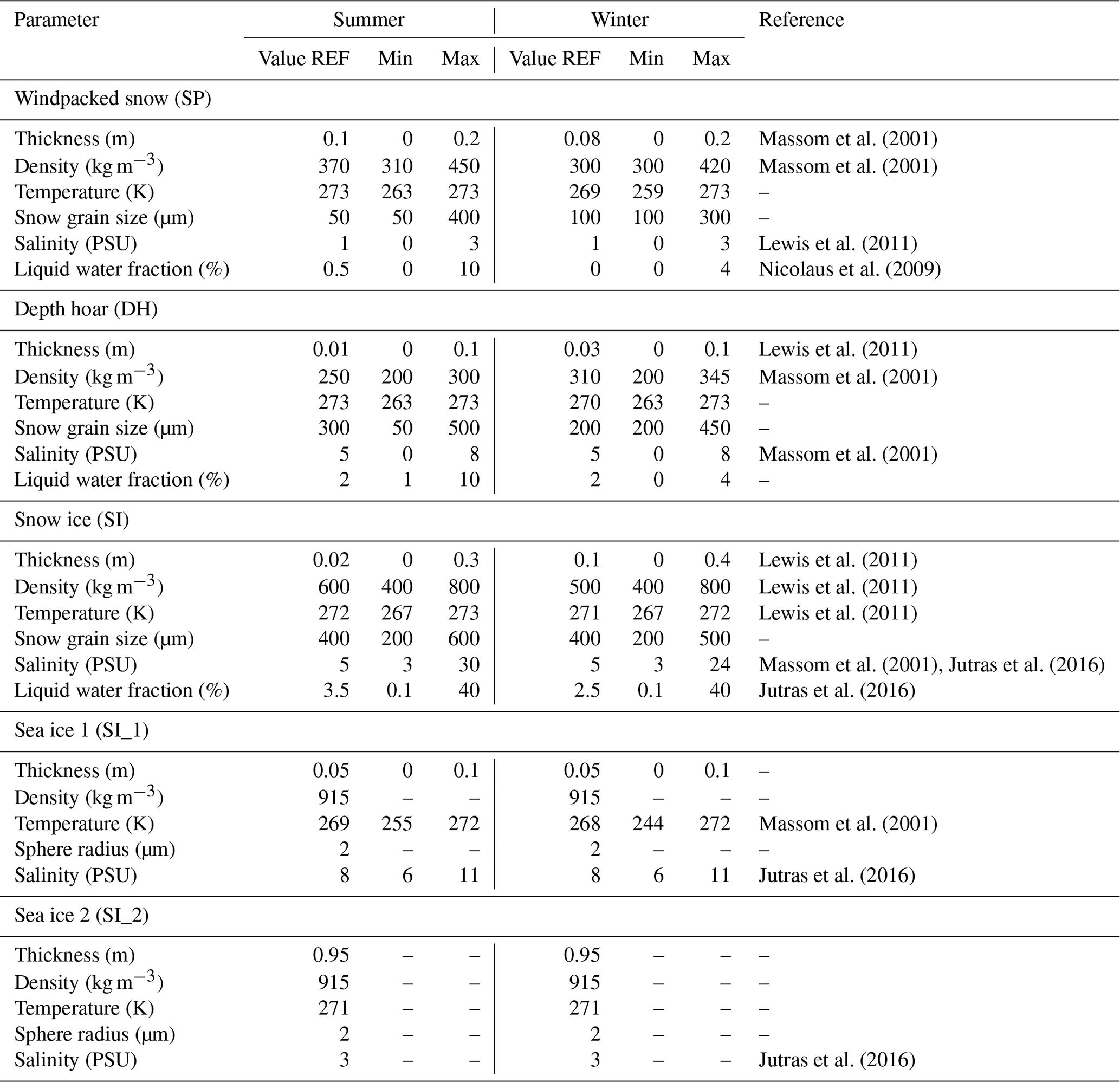
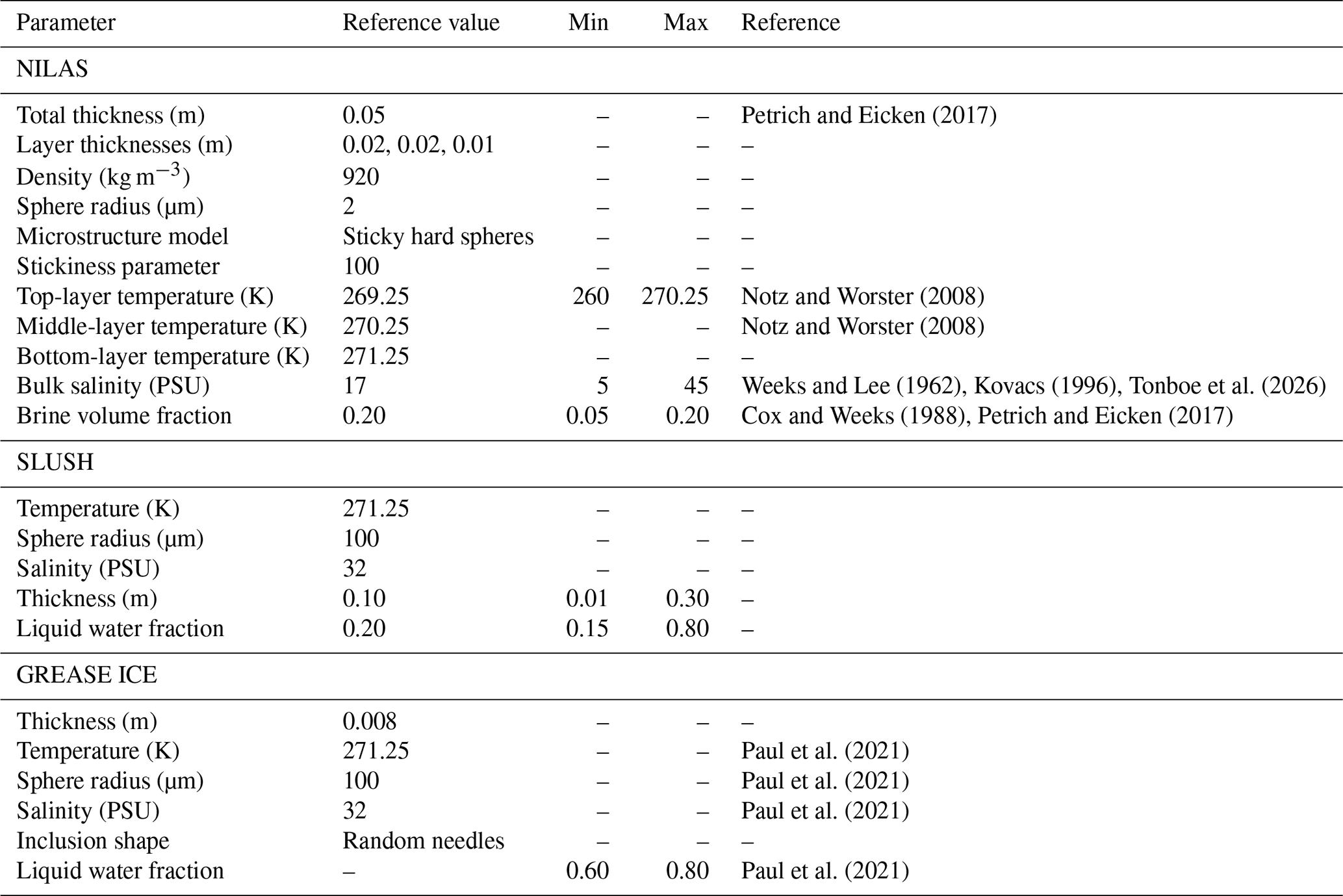
Table 2 Physical and microstructural properties of thin first-year sea ice (dark nilas), grease ice, and slush used in the SMRT sensitivity analysis. Reference values are used when a parameter is held fixed; Min and Max indicate the range swept when that parameter is varied.

Both layers of sea ice use the type “first-year ice” defined in SMRT. The brine volume fraction of the sea ice is not prescribed directly but is computed internally from temperature and salinity following the Leppäranta and Manninen (1988) formulation based on Cox and Weeks (1983) coefficient. The thick sea ice layer in contact with the ocean is characterised by a vertical temperature gradient characteristic of first-year ice (Lewis et al., 2011), described by linear interpolation between the sea ice layer on the top (SI_1) and the temperature of the ice in contact with the ocean (271 K in Table 1).

The snowpack layer ordering follows the sequence listed in Table 1.

3.1.2 Dark nilas, slush, and grease simulation

Dark nilas is represented in SMRT as a stack of three layers with physical characteristics described in Table 2 where the fixed bulk salinity corresponds to the mid-range value for newly formed ice of this thickness (Weeks and Lee, 1962; Kovacs, 1996). A vertical temperature gradient is prescribed across the layers (Table 2), where the intermediate layer temperature is interpolated linearly between the two boundary values. The brine volume fraction is fixed, across all three layers, at 0.2 (value computed at 269 K, representative of near-freezing temperatures characteristic of ice in the first hours after formation, following Leppäranta and Manninen, 1988).

Slush is modelled using the newly introduced make_slush function in SMRT, which generates a saturated layer composed of a mixture of saline water and ice with no air inclusions.

Grease ice is represented as a thin slush layer consisting of saline water, and frazil ice crystals described with an elongated needle geometry (Comiso, 2010). This geometry influences the absorption coefficient but not the scattering. The water temperature is held constant at 271.25 K (Paul et al., 2021). Coherently with the other simulations we use DORT, but for the thin layer of grease, we enabled the coherent layer processing (Mätzler and Wiesmann, 2012; Montpetit et al., 2013).

3.2 Ocean brightness temperature simulation

We use PARMIO model (Dinnat et al., 2023), to simulate the ocean T_B at 19 and 37 GHz. PARMIO models the emissivity of a flat ocean using Fresnel coefficients driven by the seawater permittivity model from Meissner and Wentz (2004). Ocean surface waves represented through Elfouhaily et al. (1997) wave spectrum multiplied by a factor 1.25 contribute to the T_B perturbation and are simulated with a two-scale model. The scattering of small waves, which are less than 4 times the radiometer wavelength, is calculated with the Small Perturbation Method (SPM) while the scattering of the large waves is calculated with the geometrical optics (GO) model. The small waves are taken into account in the Donelan et al. (1993) description for the drag coefficient, while the large waves impact through the Elfouhaily et al. (1997) sea spectrum model. A further contribution comes from the foam-covered layer where the foam fraction follows Monahan and Lu (1990) and the foam emissivity, the Yin formulation (Yin et al., 2016). The foam fraction varies as a function of wind speed. The output incorporates both the foam impact and the atmospheric contribution as included in the PARMIO model, for the ocean reference we choose a wind speed of 15 m s⁻¹. The warm and cold season reference configurations differ in the sea surface temperature (SST): 273 and 271 K respectively.

3.3 Atmosphere brightness temperature simulation

This work employs two different atmospheric models for different analysis. We use the PARMIO model to simulate a clear-sky atmosphere. PARMIO relies on an analytical atmospheric formulation that works worldwide, with the SST as the only input parameter and with constant relative humidity, which is used to compute absolute humidity and water vapour content at each atmospheric layer. The absorption is calculated layer by layer according to the model’s built-in vertical profile. This configuration does not include any varying humidity field or additional atmospheric variability. The second atmosphere we employ is simulated with the PyRTLib package (Larosa et al., 2024) embedded in SMRT, which enables the simulation of observations, under a non-scattering Rayleigh approximation for the selected radiometer. The atmospheric vertical profile is from the ERA5 reanalysis (Hersbach et al., 2020) including pressure, air temperature, water vapour (specific and relative humidity), cloud liquid and ice water and ozone of the given date, latitude and longitude of interest. These data are used to estimate the upwelling and downwelling temperature and the transmission in SMRT by selecting the R20 gas absorption model (Meshkov and De Lucia, 2007; Makarov et al., 2011), which provides recently updated gas absorption characteristics, particularly for water vapour and oxygen.

3.4 AMSR2 passive microwave observations

Advanced Microwave Scanning Radiometer2 (AMSR2) data are extracted from the unified collection of AMSR sensors, NSIDC DAAC Advanced Microwave Scanning Radiometer Unified AMSR-U (Meier et al., 2017). AMSR2, aboard the Japanese satellite Global Change Observation Mission 1st-Water, “SHIZUKU” (GCOM-W1), provided observations from July 2012. These products include observed T_B and estimated SIC for both ascending and descending orbits. The SIC and T_B are provided on a Southern Hemisphere polar stereographic grid (WGS 84/Antarctic Polar Stereographic, EPSG: 3031) at 12.5 km resolution, with a standard parallel at −71° S and central meridian at 0°. We use T_B at 19 and 37 GHz in vertical polarisation in the ascending orbit under an angle of incidence of 55°.

We applied a mask to the dataset to select the sea ice area and a limited portion of adjacent open ocean. The mask was created, for each date using the sea ice concentration (SIC > 0 %), and extending it 100 km into the ocean with a circular buffer.

3.5 Microwave brightness temperature modelling across the marginal ice zone: variability of sea ice observations

The first part of this work analyses the spread observed in AMSR2 brightness temperature within the 19–37 V space. The field-of-view brightness temperature is obtained as the area-weighted linear combination of the point-model outputs (SMRT, Sect. 3.1.1 and PARMIO, Sect. 3.2), which follows directly from the additivity of radiance. Each T_B derives from different surface types, and the weights are given by the SIC. This mixing of two 1D model outputs assumes that the vertical extent of the medium (in this context, the sea ice freeboard) is negligible compared to its horizontal extent, and that microwave wavelengths are short relative to any three-dimensional structures present. These assumptions imply that lateral and three-dimensional radiative effects, such as those caused by ice deformation or ridging, are not addressed in this work.

In the first step, we determine the reference tie points: for each season – the warm season (December to February) and the cold season (June to August) – we select dates at 15 d intervals over the period 2012–2024, yielding 96 dates per season. This multi-date circumpolar background allows us to identify the regions of the T_B space corresponding to 0 % and 100 % sea-ice concentration from AMSR2 observations.

The initialization of the physical parameters and their variation range is then informed by literature (Massom et al., 2001; Nicolaus et al., 2009; Lewis et al., 2011; Jutras et al., 2016; Soriot et al., 2022; Lawrence et al., 2024) as shown in Table 1. On this basis, we look for the set of parameters whose forward modelled T_B better reproduces the two AMSR2–observed tie points for the two extreme surface conditions (0 % and 100 % SIC).

The resulting reference simulations define the seasonal circumpolar tie points T_SI and T_OO in Eq. (1), representative of mean seasonal conditions rather than the precise daily condition: the first-year sea ice simulation (point X_A in Fig. 1), described through the reference values in Table 1 and Sect. 3.1.1 and the ocean simulation (point X_OO in Fig. 1), described in Sect. 3.2.

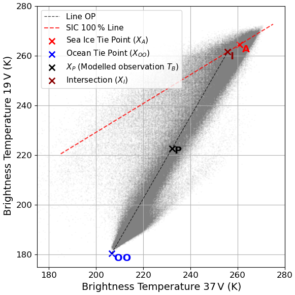
Figure 1 SIC retrieval algorithm description. Brightness temperature at 19 versus 37 V from AMSR2 observations (black dots). X_A and X_OO are, respectively, the tie points for 100 % SIC sea ice (SMRT output for first-year ice) and open ocean (PARMIO output). The top line through tie point X_A (red dashed line) is the linear regression of the 100 % SIC cluster. Point X_P is an observational modelled point at true 50 % SIC (output of SMRT warm season reference snowpack with dry windpacked snow layer). Line OP (dashed black line) through the ocean tie point and the observation point intercepts SIC 100 % line in X_I.

In the second step, we iteratively vary each parameter quantitatively across the range in Table 1, while keeping all others constant at their reference value (Table 1). The parameter range is sampled using 21 evenly spaced values, with a uniform increment. Note that the liquid water fraction sensitivity analysis is performed at a fixed temperature of 273 K.

Finally, in the third step, the sea ice T_B obtained in the second step is combined with T_OO through a SIC-weighted linear combination, yielding mixed grid-cell simulations (e.g. points X_P, Fig. 1 ) that capture the variability observed in the seasonal AMSR2 MIZ observations for different ice types.

3.6 Sea ice concentration sensitivity analysis

3.6.1 SIC sensitivity to snow and sea ice parameters

The sensitivity analysis algorithm for each snow and sea ice physical parameter leverages the tie points X_A and X_OO and the observational point X_P, determined in Sect. 3.5 and is implemented as follows:

1. Determine the slope of the 100 % SIC line (SIC 100 % line in Fig. 1). For this, we use the least-square linear regression in the two-channel space of the 100 % SIC T_B cluster values for the analysed season.

2. Determine the intercept with the 100 % SIC line (point X_I in Fig. 1). To do so, we compute the equation for the line through the modelled observation X_P (third step of Sect. 3.5) and the ocean tie point X_OO.

3. Retrieve the SIC via geometric interpolation (Comiso, 1995, 2013), computing the ratio:

   $$\begin{array}{}\text{(3)}& \text{SIC}={\displaystyle \frac{\left|\stackrel{\mathrm{‾}}{\mathrm{OP}}\right|}{\left|\stackrel{\mathrm{‾}}{\mathrm{OI}}\right|}}=\left({\displaystyle \frac{T_{X_{\mathrm{P}}}-T_{X_{\mathrm{OO}}}}{T_{X_{\mathrm{I}}}-T_{X_{\mathrm{OO}}}}}\right),\end{array}$$

   where points X_I and X_P are determined respectively in steps 1, 2 and X_OO in Sect. 3.2.

4. For each parameter value, calculate the difference between the retrieved and prescribed true SIC.

3.6.2 SIC sensitivity to thin ice presence

For each surface type, the tie point X_A of snow-covered first-year sea ice is compared to T_B values obtained by replacing a fraction f of the total sea ice with thin ice at representative values (0 %, 15 %, 30 %, 50 %, 80 %, 100 %), with the remaining fraction (1−f) being first-year ice. The resulting T_B for the observation (X_P) is computed as a linear combination of the contributions from first-year ice, thin ice, and open ocean, weighted by their respective area fractions.

The sensitivity analysis for the thin ice–dark nilas component quantifies the impact of different thin ice fractions on the total SIC, as a function of temperature profiles, salinity profiles or brine volume fractions in the dark nilas. In the temperature sensitivity experiment for the dark nilas, the top-layer temperature is swept within the range in Table 2 (1 K increment), while the bottom layer is held at 271.25 K and the intermediate layer temperature is interpolated linearly between the two boundary values. The salinity and brine volume fraction are fixed (reference values in Table 2). In the salinity sensitivity experiment, the bulk salinity is varied for the range in Table 2 (1 PSU steps), where the maximum salinity values are recorded as extremes in Tonboe et al. (2026), the brine volume value is computed at 269 K, and all other parameters are kept constant. Finally, for the brine volume fraction sensitivity experiment, the volume fraction ranges from the lower percolation threshold (0.05–0.07, Cox and Weeks, 1988) to a maximum of 0.20 for nilas Petrich and Eicken (2017), in 0.005 increments, applied uniformly in the three layers (Table 2).

The sensitivity analysis for the slush component quantifies the impact of different slush fractions on the total SIC, as a function of thickness and liquid water fraction in slush. In the thickness sensitivity experiment, the thickness is sampled at 10 non-uniformly spaced values within the range in Table 2, with finer resolution at smaller thicknesses, while all other parameters are kept constant. In the liquid water fraction sensitivity experiment, the fraction is varied across 14 values in 5 % increments within the range in Table 2, while all other parameters are kept constant.

The sensitivity analysis for the grease ice component quantifies the impact of different grease ice fractions on the total SIC, as a function of the liquid water fraction in the grease. The liquid water fraction is varied in 5 % increments within the range in Table 2, while all other parameters are kept constant.

3.6.3 SIC sensitivity to wind speed over the ocean

The sensitivity analysis for the ocean component assesses the impact of surface T_B variations due to wind speed on SIC. To do so, we modulate the wind speed in 1 m s⁻¹ increments over a range from 2.5 to 30 m s⁻¹. The SIC sensitivity analysis is analogous to the method described in Sect. 3.6.1 with the only modification that the observational point X_P is now represented by each new combination (19–37 V) of ocean T_B resulting from a variation in the wind speed relative to the reference of 15 m s⁻¹.

3.6.4 SIC sensitivity to atmosphere variability over ocean

The sensitivity analysis of the atmosphere is conducted by applying varying atmospheric profiles over the ocean surface in SMRT. To sample the atmospheric variability throughout the warm and the cold season, profiles are extracted from ERA5 at a regular spatial grid of longitudes spaced every 60° (6 points) and latitudes at −60, −65 and −70° S (3 points). Temporally, profiles are sampled every 10 d within the warm season (here defined as January–February 2022) and cold season (June–July 2022), yielding 6 dates per month and 108 profiles per season. The surface contribution is taken from the 100 % T_B output from the PARMIO model (with the atmosphere deactivated) at wind speed of 15 m s⁻¹, consistently with the ocean simulation described in Sect. 3.2. Each atmosphere object modelled with the pyrtlib_era5_atmosphere function in SMRT is overlaid on top of the ocean medium. The resulting T_B, linearly combined with the sea ice tie point (X_A), serve as an observational point X_P to which the SIC retrieval algorithm is applied (Sect. 3.6.1).

4 Results

4.1 Sensitivity analysis in warm and cold seasons

The scatter of the observations around the line connecting the tie points (Figs. 2 and 3) is captured through the simulation obtained by varying different physical parameters in their assumed range of values (Table 1). Figure 2 shows that in the warm season, the liquid water fraction (LWF) and the snow grain size exhibit the greatest variability in the windpacked layer (Fig. 2b, c), followed by the thickness (Fig. 2f). Density, temperature and salinity changes show negligible scatter on the T_B across the snowpack layers SP and DH (Fig. 2a, d, e, g, j and k). Despite the slightly wet windpacked layer (0.5 % LWF), thickness and snow grain size changes show noticeable T_B variability, also in the underlying layers (Figs. 2i and l; 3c and f). While variability in T_B due to changes in LWF within the depth hoar layer remains limited, it increases in the snow ice layer, where LWF reaches values typical of saturated snow and slush conditions (Fig. 3b). For the two layers on the bottom (SI and SI_1), the T_B drops significantly when the layer is considered absent in the simulations (null thickness in Fig. 3f and i). The snow–ice interface temperature, represented in the top sea ice layer SI_1 temperature, shows high variability compared to the temperatures in the overlaying layers. The deeper sea ice layer does not affect the microwave signature (result not shown).

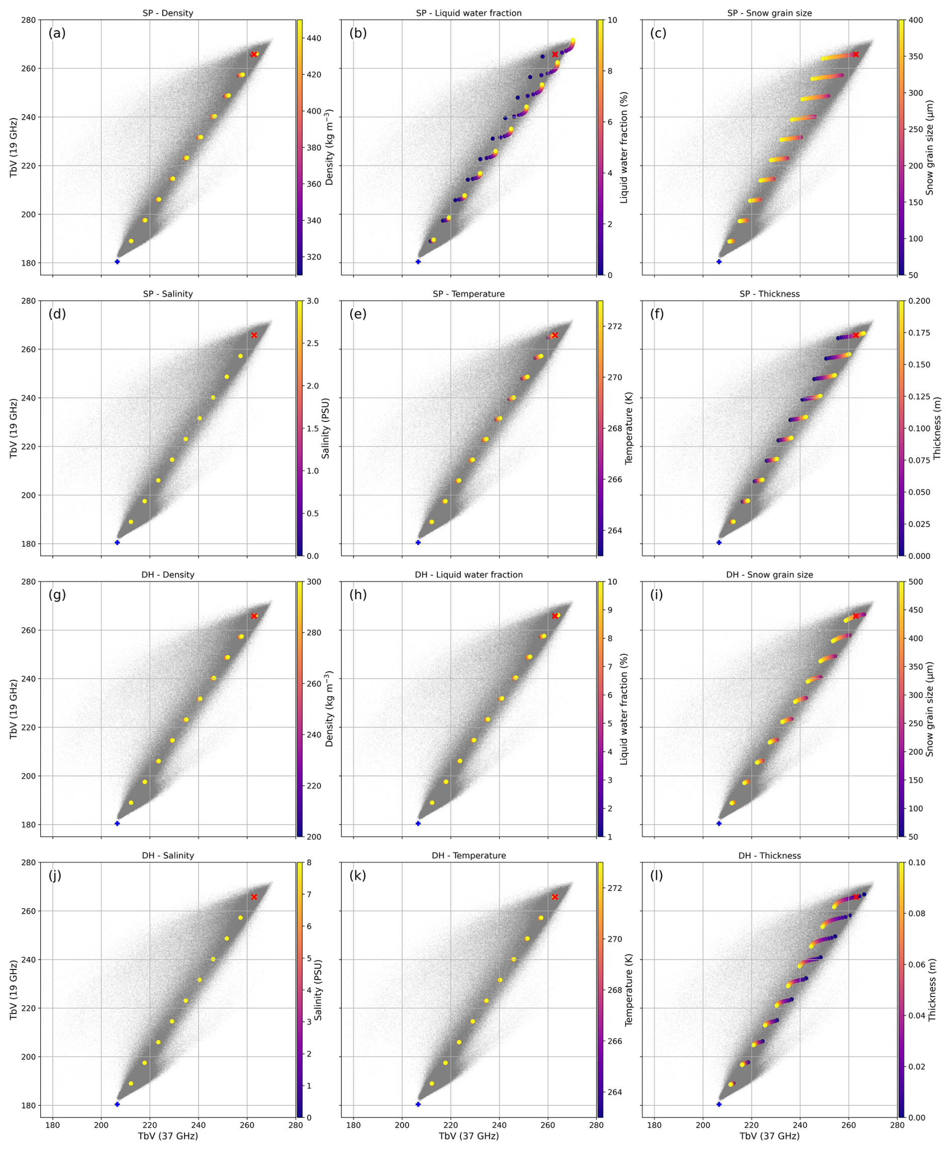
Figure 2 Brightness temperature signature in the 19–37 V space corresponding to variations in the physical properties of sea ice and snowpack layers, as obtained with the three-steps method described in Sect. 3.5. The MIZ T_B observations from AMSR2 (black dots) represent warm conditions. Each subplot examines a single parameter for a specific layer: windpacked (SP), depth hoar (DH). Data points for 100 % SIC (red cross) and open ocean (blue cross) serve as reference tie points. Each data point is coloured by parameter value and it derives from a linear SIC combination (plotted at 10 % SIC increments for T_B variability visualization) of modelled variations from the reference configuration.

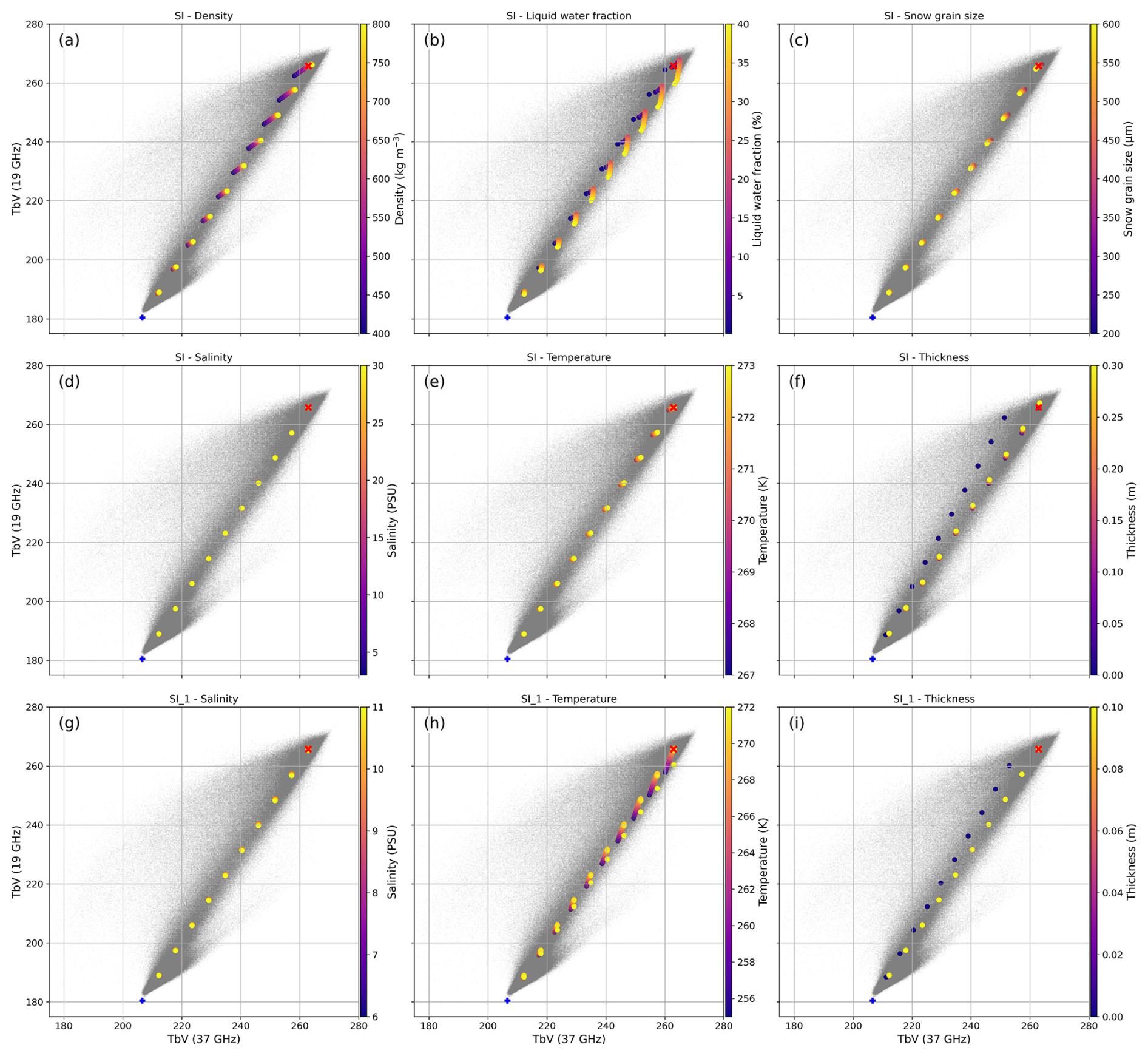
Figure 3 Brightness temperature signature in the 19–37 V space corresponding to variations in the physical properties of sea ice and snowpack layers, as obtained with the three-steps method described in Sect. 3.5. The MIZ T_B observations from AMSR2 (black dots) represent warm conditions . Each subplot examines a single parameter for a specific layer: the snow ice (SI) or top layer of first-year sea ice (SI_1). Data points for 100 % SIC (red cross) and open ocean (blue cross) serve as reference tie points. Each data point is coloured by parameter value and it derives from a linear SIC combination (plotted at 10 % SIC increments for T_B variability visualization) of modelled variations from the reference configuration.

Figure 4 shows that, in the cold season characterized by a dry windpacked, the SP top-most layer shows a more contained variability in T_B compared to the warm season (Figs. 2b, c and f; 4b, c and f).

Figure 4 Same as Fig. 2 for cold season conditions.

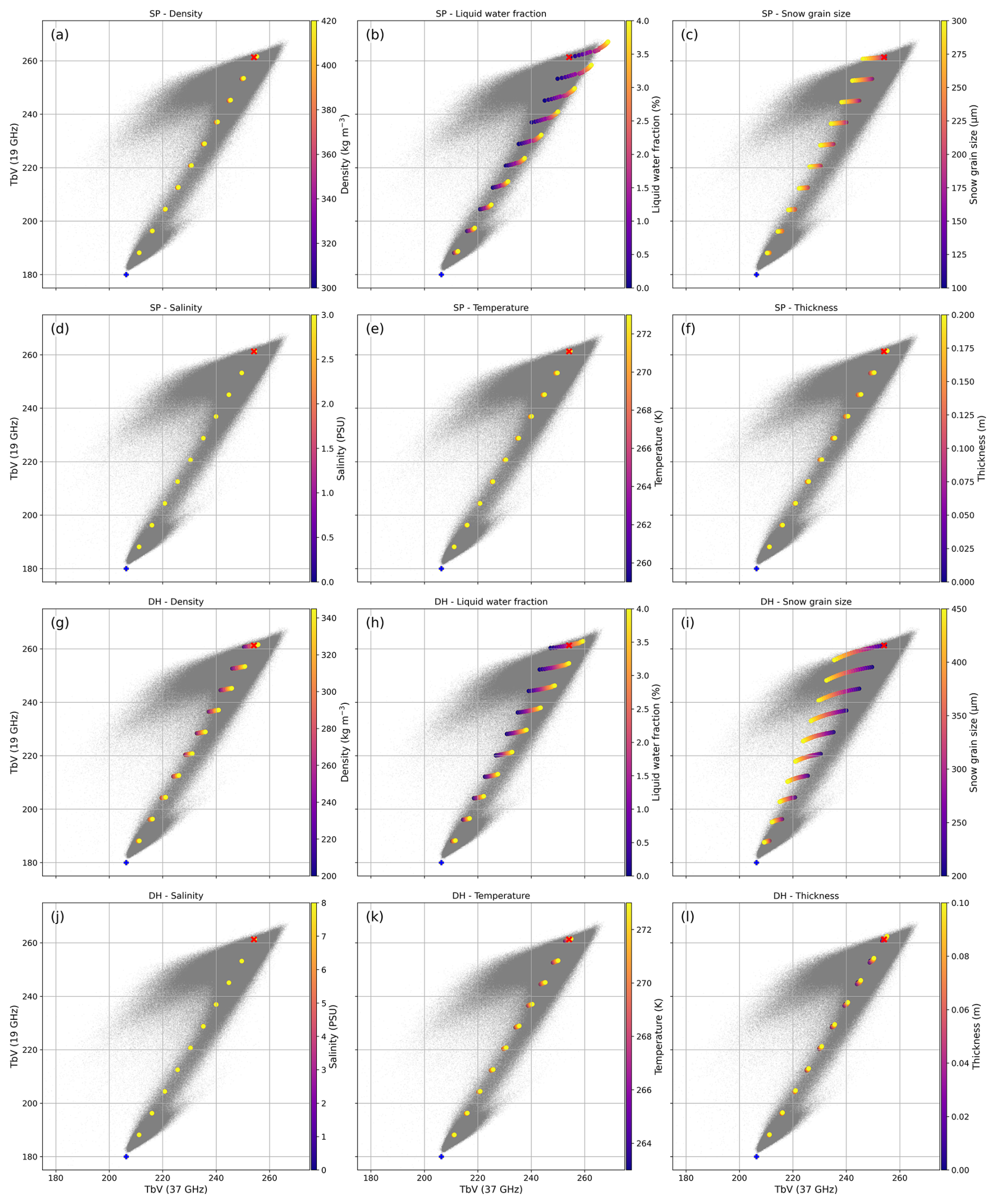
The brightness temperature shows high sensitivity to LWF and snow grain size; however, unlike the warm condition, this occurs predominantly in the DH and SI layers (Figs. 4h and i; 5b and c). Similarly to the warm season, the thickness of the bottom layers (SI and SI_1) shows different T_B when the layer is absent from the simulations (Fig. 5f and i) and the snow–ice interface temperature exhibits high T_B variability.

Figure 5 Same as Fig. 3 for cold season conditions.

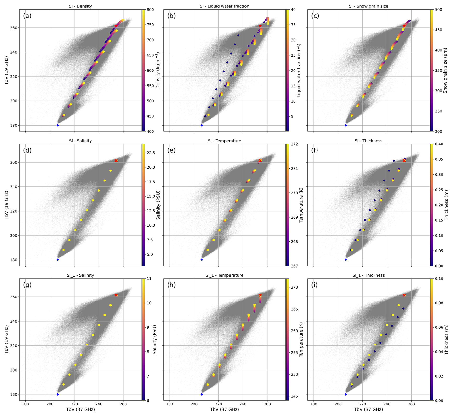
Figure 6a illustrates the impact of the wind speed on the microwave signature both with and without the foam contribution. The inclusion of foam makes this parameter a major driver of T_B variability and leads to higher scatter in the simulations. Although wind speeds up to 30 m s⁻¹ are considered in the simulations, the spread of the observations is not fully captured by the model chain. However, a significant portion of the observed cluster around the ocean tie point and its trend is reproduced in the output T_Bs with foam inclusion at 0 % SIC (Fig. 6a).

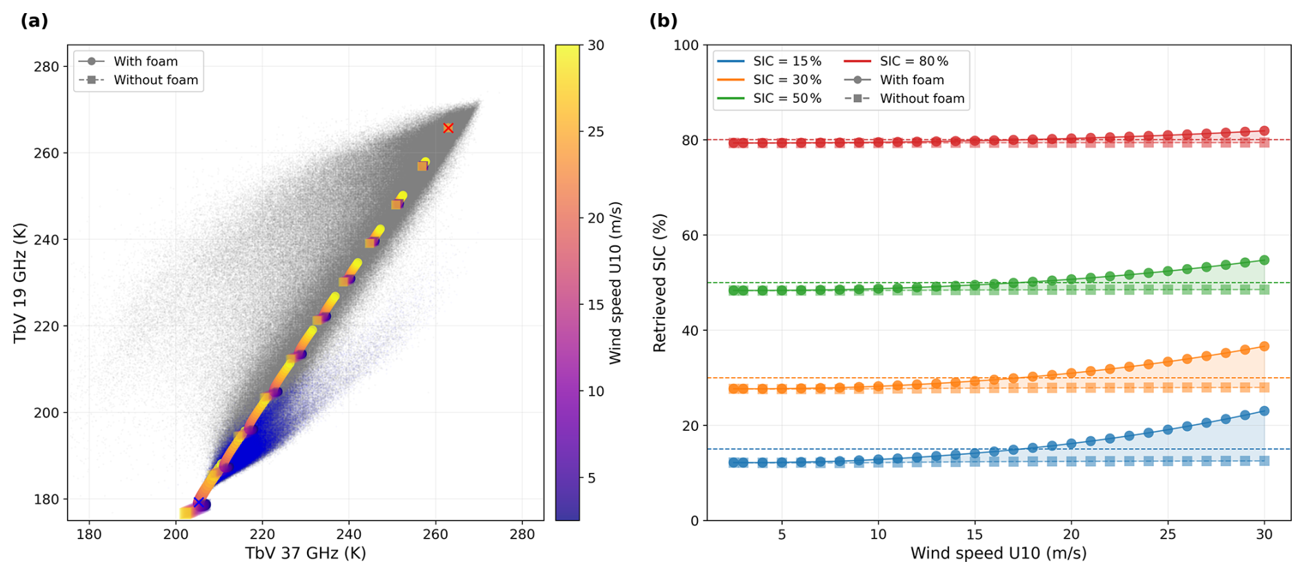
Figure 6 (a) Brightness temperature signature in the 19–37 V space corresponding to wind-induced ocean surface property variations. The MIZ T_B observations (black dots) and open ocean observations (blue dots) from AMSR2 correspond to warm conditions. Both the observation clusters are masked as described in Sect. 3.4. Each data point is coloured by wind speed value, and it derives from a SIC linear combination (shown at 10 % SIC increments). (b) Warm season. SIC retrieved for wind speed variation from the reference ocean parametrisation with foam (15 m s⁻¹). True SIC values (15 %, 30 %, 50 %, 80 % selected to represent characteristic values across the MIZ range) are shown with horizontal lines. Data points are coloured by SIC and shown for increasing wind speeds from 2 to 30 m s⁻¹. The simulations are shown both including the foam effect (circles) or not (squares).

Figure 7 shows that the atmosphere introduces high variability in the open ocean T_B, spreading the T_B across the 0 % SIC cluster, primarily with changes in the 37 V channel for both seasons.

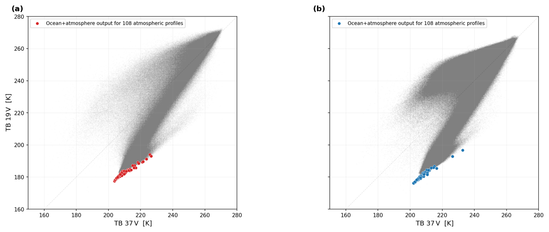
Figure 7 (a) Brightness temperature signatures in the 19–37 V space for 108 atmospheric profiles selected as described in Sect. 3.3 (warm season), superimposed on the open ocean simulation at 15 m s⁻¹ wind speed. Sea ice and ocean brightness temperature observations from AMSR2 correspond to the warm season. (b) Same as (a) for the cold season.

Figure 8 shows the scatter of the observations in the 19–37 V plane induced by the presence of dark nilas whose T_B exhibits a wide spread reaching 40 K, when the bulk salinity value is at its extreme (Fig. 8a). As shown in Fig. 8a, the thin ice T_B is closer to the sea ice tie point at low salinity values. In contrast, at high salinities, characteristic of the initial stages of sea ice growth, the T_B shifts towards the ocean tie point. Compared to the salinity case, the T_B variability is more limited and closer to the sea ice tie point, but remains significant when the changing parameters are the brine volume fraction (Fig. 8c) and the top-layer temperature (Fig. 8e).

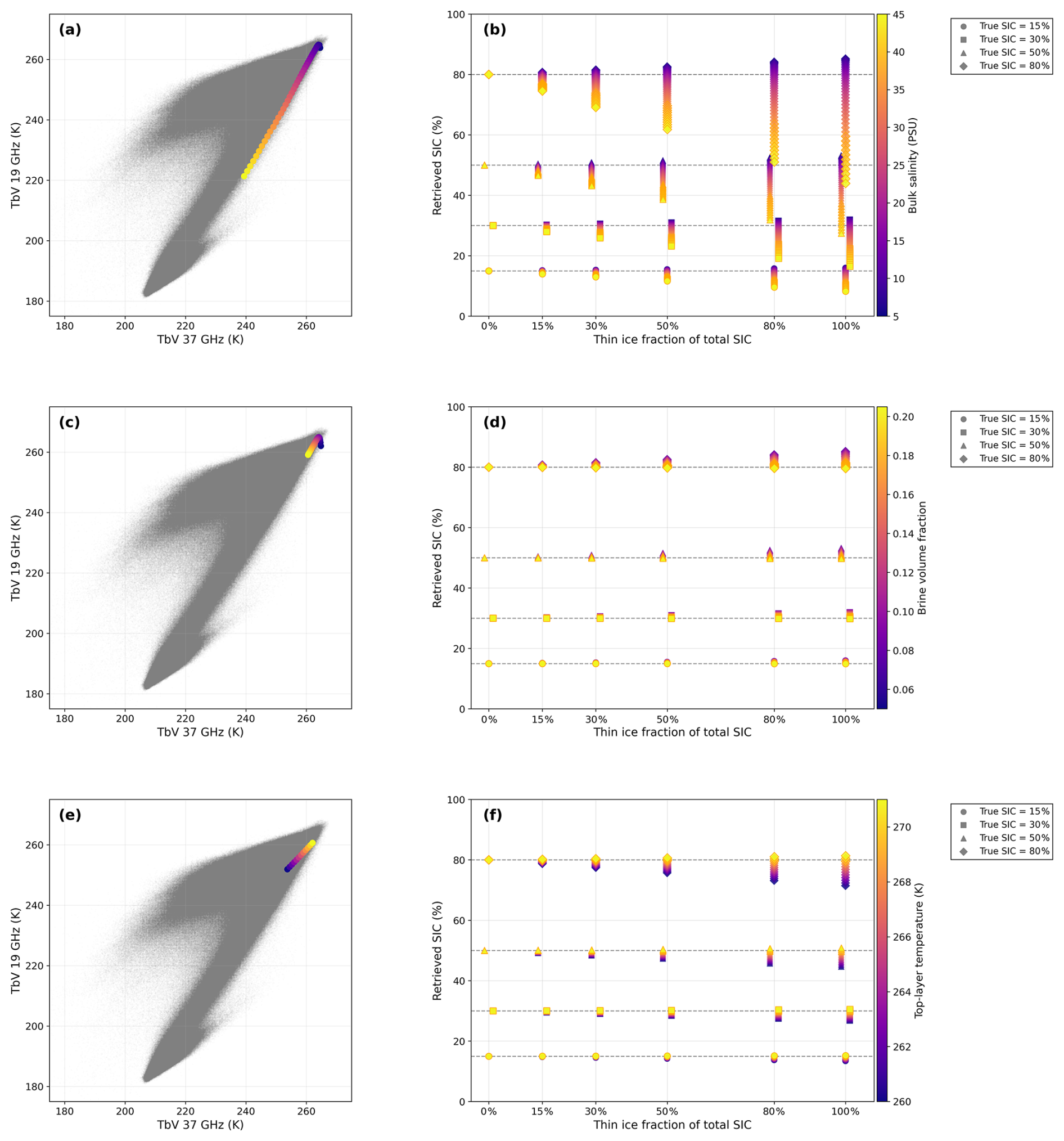
Figure 8 Brightness temperature signature in the 19–37 V space (left column; panels a, c, e) and retrieved SIC (right column; panels b, d, f) for varying proportions of dark nilas mixed with thick first-year sea ice, as obtained with the method described in Sect. 3.5.2. Rows correspond to sensitivity experiments on bulk salinity (a, b), brine volume fraction (c, d), and top-layer temperature (e, f). In the left panels, cold season AMSR2 observations (grey dots) serve as a background, and each modelled point (100 % thin ice cover) is colour-coded by the varied parameter value. In the right panels, the true SIC levels (15 %, 30 %, 50 %, 80 %) are marked by horizontal dashed lines, and retrieved SIC values are offset horizontally around each thin ice fraction for visual clarity but computed at the exact fraction values.

Figure 9 illustrates the T_B changes in the slush simulations when varying the slush layer thickness, which leads to a negligible variation in T_B (Fig. 9a) and in the liquid water fraction which, at its minimum (15 %) can yield T_B values higher than the sea ice tie point, while at its maximum (80 %) it reaches brightness temperatures close to those of the open ocean. For similarly high LWF values, typical of grease ice, the grease layer exhibits a comparable signature; it ranges from T_B values intermediate between the two tie points to those of the open ocean (Fig. 10a).

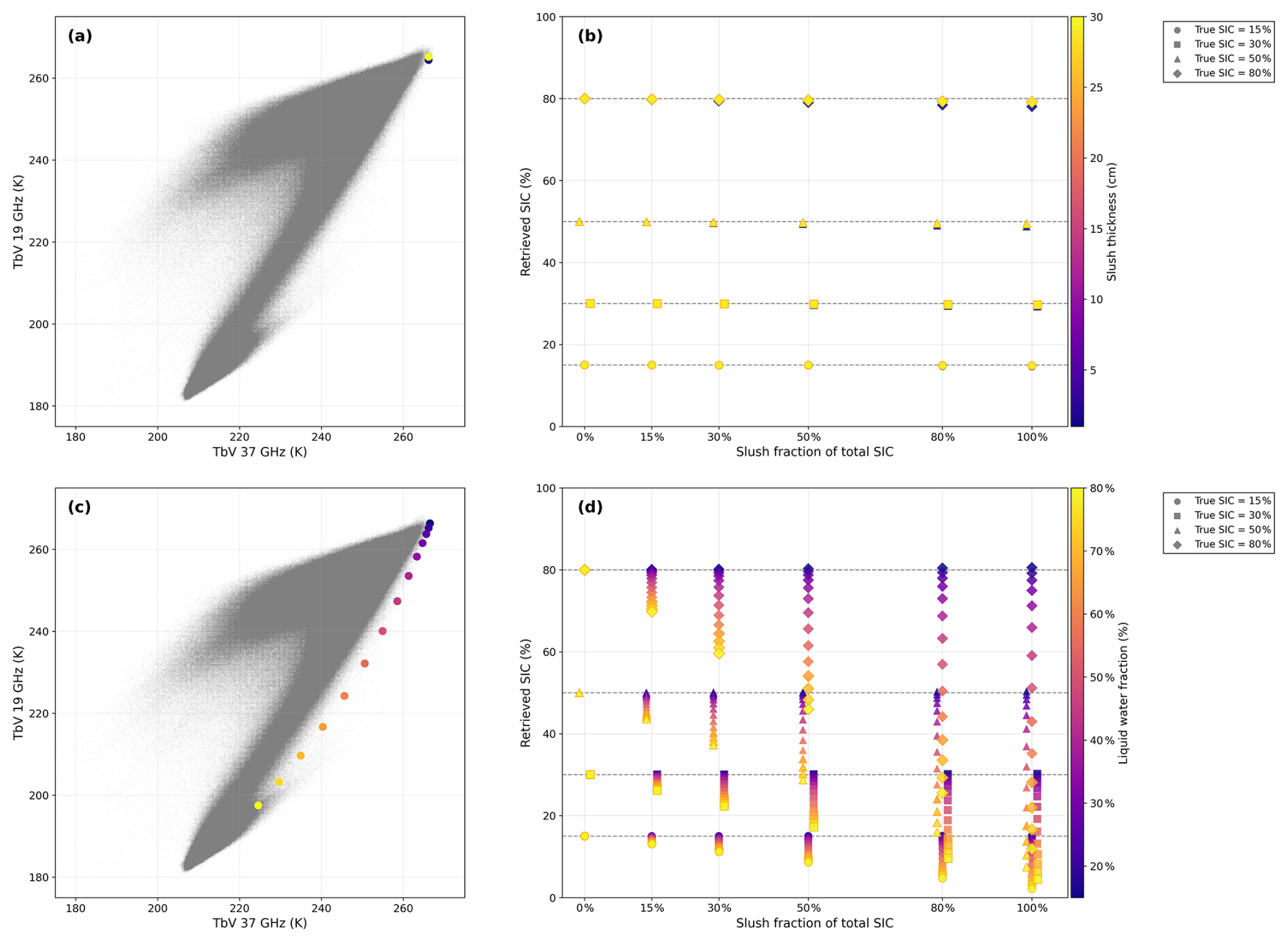
Figure 9 Brightness temperature signature in the 19–37 V space (left column; panels a, c) and retrieved SIC (right column; panels b, d) for varying proportions of slush mixed with thick first-year sea ice. Rows correspond to sensitivity experiments on slush thickness (a, b) and liquid water fraction (c, d). In the left panels, cold season AMSR2 observations (grey dots) serve as a background and each modelled point (100 % slush cover) is colour-coded by the varied parameter value. In the right panels, the true SIC levels (15 %, 30 %, 50 %, 80 %) are marked by horizontal dashed lines, and retrieved SIC values are offset horizontally around each thin ice fraction for visual clarity but computed at the exact fraction values.

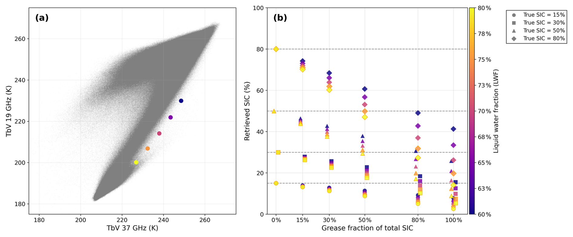
Figure 10 Brightness temperature signature in the 19–37 V space (a) and retrieved SIC (b) for varying proportions of grease ice mixed with thick first-year sea ice. In the left panel, cold season AMSR2 observations (grey dots) serve as a background and each modelled point (100 % grease cover) is colour-coded by LWF value. In the right panel, the true SIC levels (15 %, 30 %, 50 %, 80 %) are marked by horizontal dashed lines, and retrieved SIC values are offset horizontally around each thin ice fraction for visual clarity but computed at the exact fraction values.

4.2 Sea ice concentration uncertainty

In line with the sensitivity analysis (Sect. 4.1), the highest impact on the SIC retrieval uncertainty (in %), in the warm season, is primarily attributed to the thickness, LWF and the snow grain size in the SP and SI layers (Fig. 11a, d and e, blue and purple curves). While for SIC values below 50 %, LWF and snow grain size induce uncertainties smaller than 5 %; when considering SIC up to 80 %, these uncertainties reach up to 10 %. To be noted, the thickness in the snow ice layer induced an uncertainty in the retrieved SIC, mostly when the layer is completely absent (Fig. 11a).

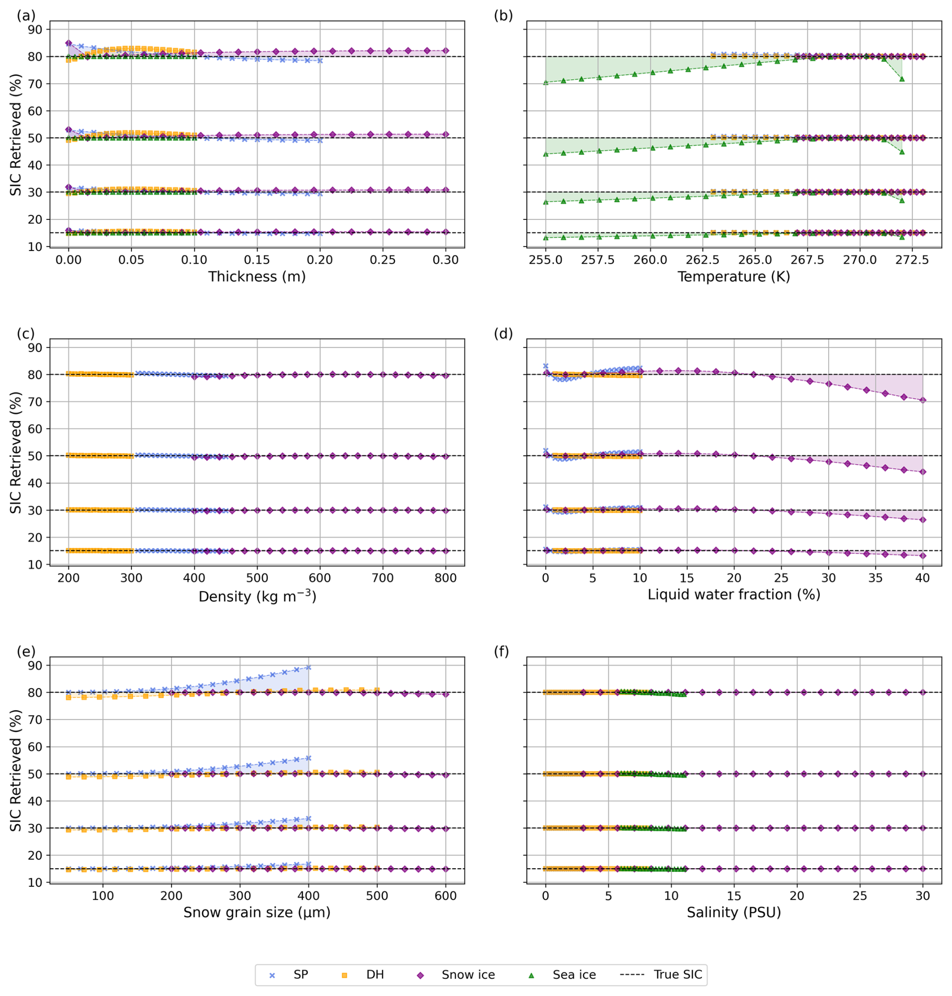
Figure 11 Warm season. SIC retrieved for individual parameter variations from the reference snowpack and sea ice. True SIC values (15 %, 30 %, 50 %, 80 % shown to represent characteristic values across the MIZ range) are represented by horizontal lines. For each layer – windpacked (SP, blue crosses), depth hoar (DH, orange squares), snow ice (SI, purple diamond), top first-year sea ice (SI_1, green triangles) – the retrieved SIC is plotted for regularly spaced values within the range defined in Table 1.

In the depth hoar layer, the thickness, snow grain size, and LWF all contribute similarly, each causing an uncertainty within 3 % (Fig. 11a, d and e, orange curve). All the parameters in the uppermost layer of sea ice show very limited impact on the SIC variability; within 1 % and 2 %, except for the snow–ice interface temperature, which is a dominating source of uncertainty in SIC. It reaches values as large as 10 % over the tested range (Fig. 11, green lines).

Figure 6b illustrates that SIC retrieval is highly sensitive to changes in the ocean surface at low SIC. When the foam is accounted for in the simulations, the uncertainty can reach values close to 10 % under strong wind conditions, up to 30 m s⁻¹ whilst at 80 % SIC it decreases to 2 %. When the foam effect is not included in the simulations, the uncertainty is negligible, indicating the foam is the driver of this uncertainty.

Figure 12a shows that during the warm season, the retrieved SIC under varying atmospheric profiles varies by up to 6 % around the 15 % true SIC value, whilst at the upper MIZ boundary the variation decreases to 1 %.

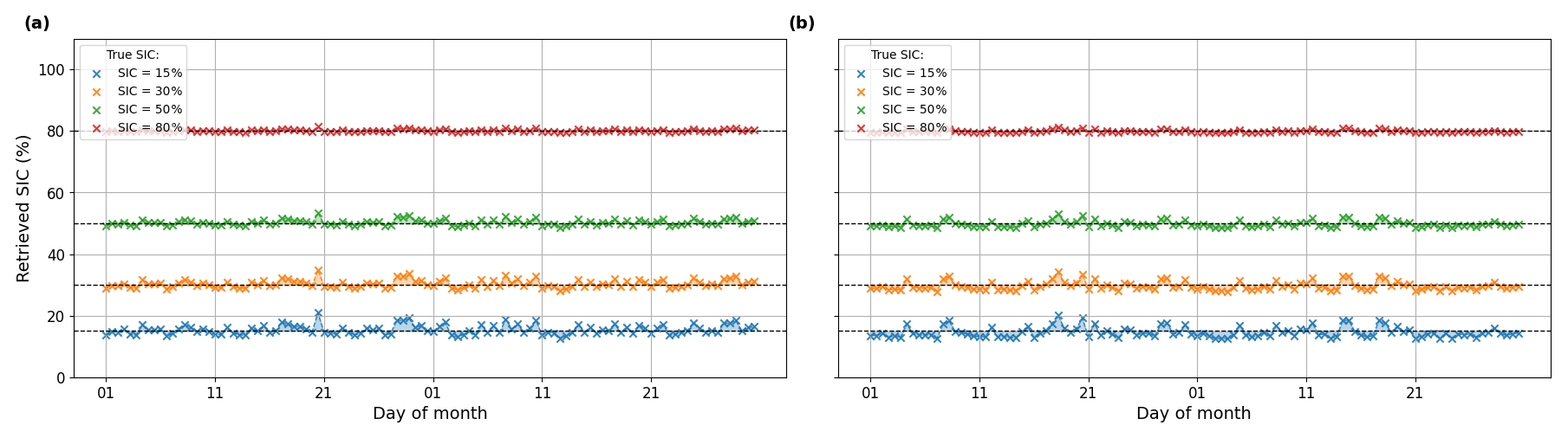
Figure 12 (a) SIC retrieved for different atmospheric profiles selected as in Sect. 3.3 for the warm season. True SIC values (15 %, 30 %, 50 %, 80 % shown to represent characteristic values across the MIZ range) are represented with horizontal lines. Data points are coloured by SIC and sampled for the atmosphere at different times and locations, ordered chronologically on the x-axis. (b) Same as (a) for the cold season.

Figure 13a, d and e show that the thickness, the liquid water fraction and the snow grain size remain the major drivers of the SIC uncertainty in the snowpack layers (SP, DH, SI) in the cold season, as in the warm season. Compared to the warm season, uncertainties in the dry SP layer are more limited; while when LWF exceeds 5 % for wet snow ice, the uncertainty on the higher SIC MIZ boundary (80 % SIC) is higher but still limited to less than 5 % (compared to 10 % in the summer season). Slightly larger is the uncertainty deriving from higher snow grain size in the DH, though this remains well within the 10 %.

Figure 13 Same as Fig. 11 for cold season conditions. The parameter range is defined in Table 1.

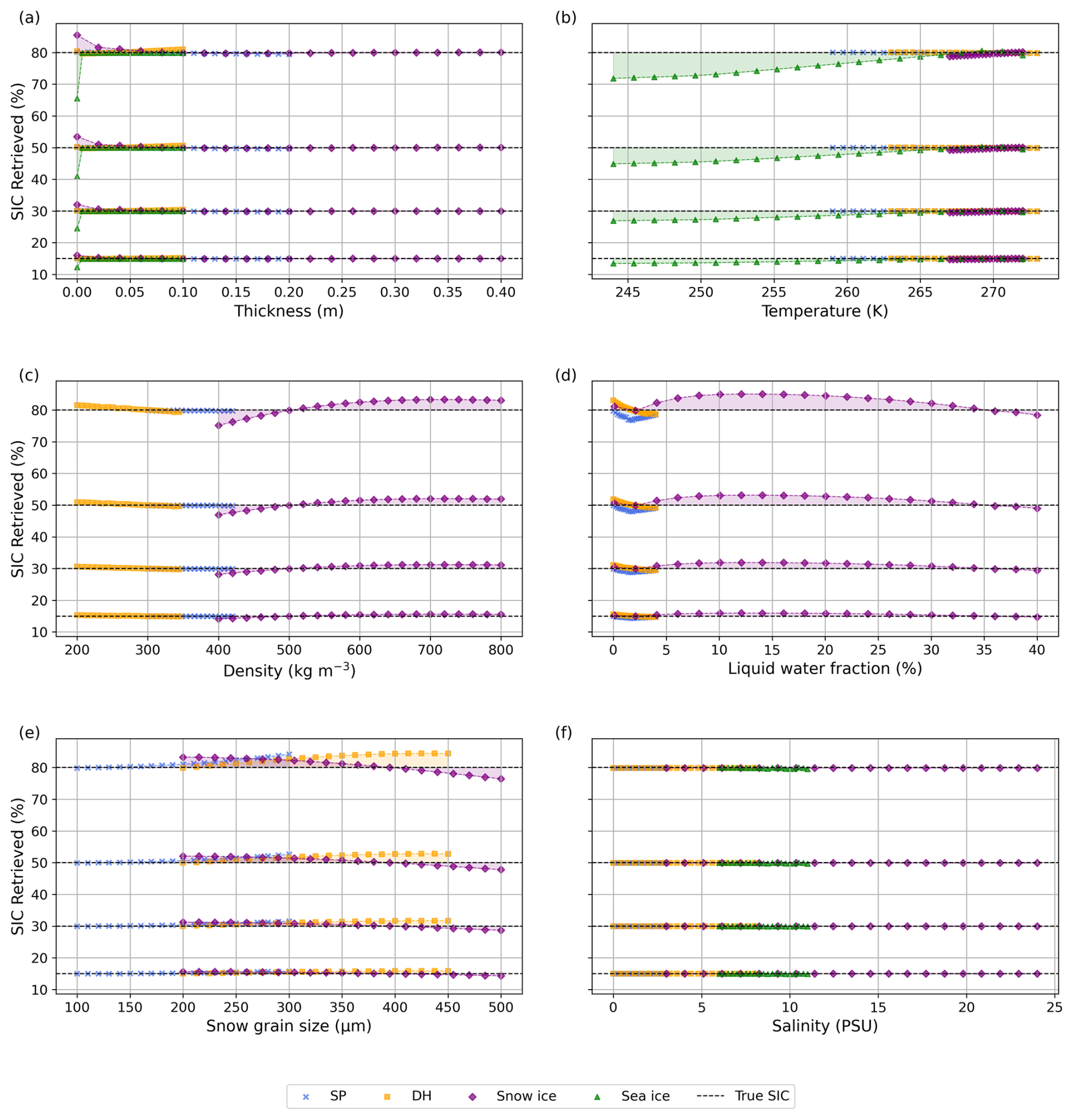
Similarly to the warm season, the thicknesses of the SI and SI_1 layers yield high SIC uncertainties when the layer thickness is null, reaching a magnitude of more than 10 % (Fig. 13a, purple and green line). SIC is insensitive to the thicknesses in the range tested, otherwise. An analogous behaviour between seasons is observed for the snow–ice interface temperature yielding uncertainties up to 10 %.

As shown in Sect. 4.1, in the cold season, T_B variations in thin ice exceed those of the snowpack on first-year ice, causing the presence of thin ice to induce substantial uncertainties in the retrieved SIC. Figure 8b shows that the inclusion of dark nilas with low bulk salinity values (minimum of 5 PSU) results in a SIC overestimation limited to 5 % when the thin ice occupies the full grid cell at 80 % SIC and it is not mixed with first-year ice. However, at the maximum tested salinity values (45 PSU), SIC retrieval underestimations can reach 35 % (Fig. 8b). In the tested range, the brine volume fraction yields to a maximum overestimation of 5 % (Fig. 8d) and the top-layer dark nilas temperature to underestimations within 10 % (Fig. 8f).

Figures 9b and d show that while slush thickness variations have a negligible impact on the retrieved SIC, the LWF can introduce high uncertainties. This means that when a grid cell at 80 % SIC is fully covered by slush, the uncertainty ranges from a small overestimation of less than 1 % at low LWF (15 %) to an underestimation of nearly 70 % at high LWF (80 %). Similarly, for grease ice, which is characterised by inherently higher LWF values, the underestimation reaches at least 40 percentage points when the grid cell is fully covered by grease at 80 % SIC (Fig. 10b).

Figure 12b shows that the uncertainties induced from different atmospheric profiles over the ocean in the cold season are comparable to those of the warm season, and limited to 6 %, at the lower MIZ boundary (15 % SIC).

5 Discussion

In this work, we have considered the variations in physical properties of the ocean surface, the atmosphere, the snowpack and sea ice, to assess their impact on the microwave signature. Our analysis identified key variables to which T_B is more sensitive, namely LWF, snow grain size, thickness and snow–ice interface temperature for the snow-covered sea ice, wind speed for the ocean and salinity and LWF for thin ice (Sect. 4.1), which lead to greater uncertainties in the SIC retrieved through the algorithm employed (Sect. 4.2). These simulations allow to reproduce the T_B changes in the 37–19 V space. The SIC uncertainties described in this work do not account for the corrections or filters applied to obtain operational SIC products. Rather, it provides an estimate of the T_B variability and the associated SIC uncertainty deriving from the microwave signature of individual surface properties prior to their processing and combination. In line with literature, the algorithm performs better when the snow is dry, characteristic of the winter season on first-year ice, compared to the summer season, and the highest uncertainties in SIC in the cold season, especially in times characterised by freezing of the ocean surface is to be attributed to thin ice types (Ivanova et al., 2015). Indeed, in the warm season, the snowpack (SP and SI layers) accounts for the greatest variation in the microwave signature, which is therefore reflected in a greater uncertainty in the retrieved SIC. In the cold season, the dry SP layer is largely transparent to microwaves, so variations in T_B in the underlying DH and SI layers become more visible and lead to higher SIC uncertainties than in the warm season, though these remain smaller than the largest uncertainties observed in summer across layers and parameters (Figs. 11, 13). An important uncertainty source, independent of the season, is the temperature at the snow–ice interface, represented, in this study, by the temperature of the top thin layer of ice (Figs. 11b, 13b, green curve). This uncertainty, in the upper MIZ limit (80 % SIC), reaches about 10 percentage points of underestimation for the lower temperature range tested, results aligned with Tonboe et al. (2022). The underestimation for warmer conditions (Fig. 11b) is due to the temperature considered, highly correlated to the brine volume fraction (Leppäranta and Manninen, 1988) when close to the freezing point.

In the cold season, the uncertainty caused by the cryospheric component is dominated by the thin ice types: dark nilas, grease and slush. The presence of these ice types produces uncertainties in the simulated SIC, significantly more influential than those from any other parameter (Meier et al., 2017), yielding important SIC underestimations (Cavalieri, 1994; Ivanova et al., 2015). A variation in the dark nilas ice fraction included in the first-year sea ice, with salinity values around 20 PSU, for instance, accounts for uncertainties 10 %–20 % larger than those generated by the other snow and sea ice parameters (Fig. 8b). This sensitivity depends on the thin ice development stage (Comiso, 2012, 2013). In this work, the thin ice development is approximated through the variability of the properties of grease ice or the top dark nilas layer, which affects the most the microwave signature at the frequencies used (Naoki et al., 2008). Specifically, the permittivity changes are governed by the LWF for grease ice and by brine for the dark nilas, which in reality vary with increasing ice thickness and age. However, in this work, thickness is varied independently, without being connected to the physical processes that drive changes in the other parameters, for instance through a thermodynamic model. This is reflected in the fact that thickness is not found to be one of the sensitive parameters within the tested range. This is likely due to the low penetration of microwave caused by high salinities and LWF typical of these new ice types, which means reduced ability to obtain true thickness information at these frequencies. As a result, changes in these properties connected to ice age, for instance indirectly through changes in brine volume, are also difficult to detect. By relying solely on the vertical polarization, the BF algorithm is comparatively less sensitive to these properties (Naoki et al., 2008).

Slush in the MIZ can be present year-round and represents a highly wet surface, characterised, in this work as an ice type highly saturated with saline water. This makes it one of the main contributors to the uncertainty near the ice edge, exceeding 20 % (Meier and Notz, 2010; Ivanova et al., 2015). This can be seen at high LWF (80 %), where the uncertainty reaches 20 percentage points at true SIC 30 % and decrease to 10 % at 15 % SIC.

These properties determine whether the T_B is closer to T_OO or T_SI, as observable in Fig. 8. As discussed by Comiso (1995) in the description of the Bootstrap algorithm in frequency mode, the radiometric signature of new and thin ice formed in the marginal ice zone typically falls below the line connecting the tie points (X_OO and X_A), occupying an intermediate region between the open-water and thick-ice signatures as it can be seen in all the thin ice types modelled (Figs. 8, 9, 10). This means that the presence of newly formed thin ice (thickness < 0.3 m) yields lower brightness temperatures associated which cause a lower estimate of SIC through any employed SIC retrieval algorithm (Tonboe et al., 2022), and the presence of thin ice disrupts the linear relationship for the SIC, yielding a nonlinear 100 % SIC line. In general, the observed variability already present in a single ice type, combined with the fact that a field of view includes multiple ice types (Tonboe, 2010) whose T_B scatter does not follow the SIC isolines, makes the BF algorithm particularly sensitive to the non-linear distribution along the ice line of T_B in these frequency channels (Lavergne et al., 2019; Tonboe et al., 2022).

The impact of ocean surface variations on the retrieved SIC is limited when approaching areas of consolidated ice (SIC > 80 %) (Fig. 6b). However, when considering the ice edge (15 %–30 %), the uncertainty in the SIC retrieved can be up to 10 %, which confirms the difficulty in determining the ice edge (spurious positive SIC), and in providing an accurate SIC estimation under rough ocean surface conditions (Oelke, 1997; Meier and Stroeve, 2008; Comiso, 2013), and therefore increased emissivity (Oelke, 1997). In addition, these results are limited by the reliability of the models, especially at high wind speeds. PARMIO achieves higher accuracy with wind speed up to 15 m s⁻¹ where the model has a bias in T_B that corresponds to an underestimation within 5 K with respect to the observations. Nevertheless, Fig. 6 shows consistency between our simulated ocean T_B and the AMSR2 observations. Under clear sky conditions, considering the wind speed effect alone, the inclusion of foam brings this parameter to be among the dominant contributions to the SIC uncertainty in our simulations (Fig. 6b). On the other hand, simulations excluding foam show very limited variations even in conditions close to open water, in line with the trend presented in Andersen et al. (2006). This likely reflects the two different consequences of increasing wind speed: the impact, mostly on the H-polarised channel due to the roughness, to which the BF algorithm is insensitive, and the change of permittivity in the surface layer caused by foam air bubbles (relevant from wind speeds over 8 m s⁻¹), which leads to an increase in the V-polarised channel (Kern, 2004), of interest in the BF algorithm.

The sensitivity analysis of the atmosphere is conducted over the ocean, where atmospheric effects are more pronounced than over consolidated ice (Andersen et al., 2006). The uncertainty due to the atmosphere is just above 5 %, at the lower SIC limit of the MIZ, in agreement with the Oelke (1997) results showing that the combined effect of cloud and vapour pressure yields an overestimation of T_B (Andersen et al., 2006) and therefore to uncertainties within 10 %, which is usually less than the sum of the independent uncertainties.

A first limitation of our analysis is that it treats parameters independently. This conceals potential compensating effects contributing to the SIC uncertainty (Andersen et al., 2006). For example, the LWF sensitivity analysis conducted with clear sky atmospheric conditions can have an opposite effect on T_B, yielding smaller SIC uncertainties, however these sensitivity were tested independently. Furthermore, the parameter ranges simulated are broad, meaning that in some cases, the extreme values do not correspond to physically consistent combinations given that they are not constrained to co-vary with one another. Extensions of this work should consider simultaneous variations and their propagation on the SIC retrieval, providing further accuracy to its estimate in the MIZ. This remains, however, a challenge, given the difficulty in identifying and defining the relevant atmosphere–sea ice–ocean interactions to include in thermodynamic models, and the difficulty of measuring them in the field, especially in the MIZ.

A second limitation of our forward modelling approach is that we assume a single observations background across the entire MIZ, thereby not accounting for regional-scale heterogeneity in the snow, ocean, and sea ice. The tie points are similarly determined circumpolarly, as in the Bootstrap algorithm. This circumpolar aggregation allows us to include a wide range of parameters describing the conditions encountered in the Antarctic MIZ; however, it also means that aggregated conditions do not capture the sector-specific characteristics of Antarctic sea ice (Raphael and Hobbs, 2014). Future development of this work should focus on a finer-scale analysis to capture the changes in the physical properties that could otherwise be concealed or averaged, preventing the actual estimation of SIC. This could include a comparison against true, sector-specific observations.

A remaining challenge concerns the difficulty of modelling the variety of newly formed ice types present in the MIZ, such as pancake ice, for current microwave emission models; therefore, this applies to SMRT.

Another limitation stems from the difficulty of capturing, in the microwave signature interpretation, the strong seasonality of the sea ice characteristics (Comiso et al., 2003). Key processes include snow accumulation and metamorphism leading to intense layering typical of the Antarctic sea ice (Massom et al., 2001; Nicolaus et al., 2009; Toyota et al., 2011), surface flooding or, dynamic emissivity profiles for the thin ice depending on its age and thickness (Comiso and Steffen, 2001; Notz and Worster, 2009). Nevertheless, these processes, exert the largest influence mainly on the polarisation ratio (Cavalieri et al., 1984) which is not used in our method.

Finally, this study is restricted to address only a sensitivity analysis of the geophysical noise, represented by the variability of brightness temperatures around the open-ocean and 100 % SIC tie points and does not address additional sources of uncertainty related to spatial smearing (Lavergne et al., 2019) described in Sect.2.

6 Conclusions

This study investigated the sensitivity of the Bootstrap passive microwave sea-ice concentration retrieval to a set of environmental parameters, including snow, sea-ice, atmosphere and ocean physical properties, in the Antarctic MIZ, with the aim to better understand the sources of retrieval uncertainty.

We show that the dominant sources of uncertainty in the warm season are the liquid water fraction and the snow grain size in the snowpack, for high SIC in the MIZ, while the presence of slush is dominant near the MIZ edge. In this region, another large component in the SIC uncertainty is the ocean surface, and its combined contribution with that of the atmosphere. The largest effect is due to the high wind speed, leading to the presence of foam in grid cells with a high open ocean fraction.

In the cold season, the T_B of the dry snow-covered sea ice, undergoes less variation than in the warm season; however, all the thin ice types represent the most significant source of uncertainty. More specifically, lower SIC retrieval accuracy in this season is due to the high salinity and liquid water fraction present in the new ice types like grease, dark nilas (thickness  < 0.05 m) or flooded new ice (slush, thickness < 0.3 m).

Our results, derived from the application of a novel forward modelling approach to simulate mixed grid cells, provide order-of-magnitude quantification of how variations in physical parameter impact SIC retrievals across different sea ice concentrations in the MIZ.