Data-driven equation discovery of a sea ice albedo parametrisation

In many sea ice models, a single-category, zero layer thermodynamic scheme is employed, in which sea ice albedo is prescribed based on surface types depending on snow cover, surface temperature, or sea ice thickness. The Parkinson and Washington parametrisation (PW79) is a commonly used one, which assigns four constant albedo values corresponding to distinct surface types. This parametrisation is too simple to capture the spatiotemporal variability of observed sea ice albedo. Here, we aim for an improved parametrisation by discovering an interpretable, physically consistent equation for sea ice albedo using symbolic regression, an interpretable machine learning technique, combined with physical constraints. Leveraging daily pan-Arctic satellite and reanalyses data from 2013–2020 – dominated by conditions representative of the Central Arctic – we apply sequential feature selection which identifies snow depth, surface temperature, sea ice thickness and 2 m air temperature as the most informative features for sea ice albedo. As a function of these features, our data-driven equation identifies two critical mechanisms for determining sea ice albedo: the high sensitivity of sea ice albedo to small changes in thin snow and a weighted difference of the sea ice surface and 2 m air temperature, serving as a seasonal proxy that indicates the transition between melting and freezing conditions. To understand how additional model complexity reduces errors, we evaluate our discovered equation against baseline models with different complexities, such as multilayer perceptron neural networks (NNs) and polynomials on an error-complexity plane, showing that the equation excels in balancing error and complexity and reduces the mean squared error by about 51 % compared to PW79. Unlike NNs, our discovered equation allows for further regional and seasonal analyses due to its inherent interpretability. When fine-tuning its coefficients offline on regional or seasonal subsets, we uncover differences in physical conditions that drive sea ice albedo. As a use case, we further assess the Barents Sea as a contrasting sea ice regime compared to the Central Arctic, showing that the functional form of the equation remains transferable across different sea ice regimes. This study demonstrates that learning an equation from observational data can deepen the process-level understanding of the Arctic Ocean’s surface radiative budget and improve climate projections.

1 Introduction

Sea ice, formed from frozen sea water, modulates the transfer of heat, moisture, and momentum between the ocean and the atmosphere (Stroeve and Notz, 2018). During spring and summer, its high albedo allows it to reflect a large amount of incoming solar radiation, whereas during winter, it insulates the colder atmosphere from the relatively warm ocean (Hunke et al., 2010). In recent decades, observations have shown a decrease in the extent and thickness of Arctic sea ice (Kwok, 2018). Most Coupled Model Intercomparison Project Phase 6 (CMIP6) models (Eyring et al., 2016) project the disappearance of multiyear ice, i.e. ice that remains for at least one summer, before 2050 in all CO₂ emission scenarios (Notz and Community, 2020). Neglecting microstructural features such as salinity or atmospheric aerosols, thinner and younger sea ice, prevalent due to these changes, has a lower albedo (Grenfell, 1979), which leads to a higher absorption of the solar radiation by the sea ice surface, thereby promoting sea ice melting and the formation of melt ponds (Perovich et al., 2002; Light et al., 2022; Niehaus et al., 2025). The loss of sea ice exposes the darker ocean, increasing solar absorption and accelerates the melting of remaining ice (Curry et al., 1995; Stroeve and Notz, 2018). This cycle, termed the ice-albedo feedback, is the second leading feedback mechanism for Arctic amplification, following the lapse-rate feedback (Pithan and Mauritsen, 2014).

However, a wide spread remains in the projections of Arctic sea ice extent and volume across all CMIP6 models and little improvement in overall model performance has been achieved along the previous CMIP phases (Selivanova et al., 2024). One of the main sources of uncertainty in projecting Arctic sea ice is the representation of sea ice albedo, which has been oversimplified in Earth System Models (ESMs) (Curry et al., 2001; Pirazzini, 2009). Over the past decades, sea ice albedo parametrisations of various complexities have been developed by incorporating spectral band dependencies (Holland et al., 2012), cloud conditions (Jäkel et al., 2024), and explicitly resolving melt ponds (Flocco et al., 2010; Hunke et al., 2013). More sophisticated models use sea ice radiative transfer schemes that compute an albedo from inherent optical properties, including those of ice, snow, ponds, and included absorbers (black carbon, algae) instead of prescribing an albedo based on surface type (Briegleb and Light, 2007; Holland et al., 2012).

Trading accuracy or more complex physics for simplicity and lower computational cost, many sea ice models employ simplified sea ice albedo parametrisations. As an example, the Finite-Element Sea Ice Model (FESIM; Danilov et al., 2015), part of the Alfred Wegener Institute Climate Model (AWI-CM3; Streffing et al., 2022), employs a very simplified sea ice albedo parametrisation based on Parkinson and Washington (1979, hereafter PW79). In FESIM, PW79 is augmented with an implicit treatment of melt ponds by distinguishing between melting and non-melting conditions. Fixed broadband albedo values (α) are assigned to four surface types: snow-covered ice (α=0.81), bare ice (α=0.7), wet (melting) snow (α=0.77), and wet (melting) ice (α=0.68). Following a zero-layer thermodynamic scheme (Parkinson and Washington, 1979), FESIM uses these four values as tuning parameters to compensate for other biases within the model. Thus, the spatiotemporal variability of sea ice albedo is not captured in its full complexity. We argue that a more realistic formulation of sea ice albedo is needed to disentangle model errors resulting from the thermodynamic scheme.

Machine learning (ML) has become a pivotal tool in Earth system science. The era of big data originating from a diversity of observational products, reanalyses and climate data from CMIP models provides high-dimensional datasets that ML can leverage to reveal hidden patterns and accelerate discoveries beyond conventional approaches (Eyring et al., 2024; Vance et al., 2024; Bracco et al., 2024; Camps-Valls et al., 2023). In particular, data-driven equation discovery, an interpretable ML method, has the potential to bridge the gap between the ML and Earth system science community by providing transparency and reliability in ML predictions. Analytical expressions identified from data allow the user to interpret the ML prediction ad hoc, providing trustworthiness in the decision-making process of the ML algorithm and advancing scientific discoveries (Huntingford et al., 2025; Song et al., 2024). Use cases in Earth system modelling focus on improving the representation of subgrid processes, such as the representation of clouds (Grundner et al., 2024) and ocean eddies (Zanna and Bolton, 2020). Integrating ML with physical modelling aims to create hybrid Earth system models (ESMs) that combine traditional physics-based frameworks with data-driven methods, offering a promising pathway to improve climate projections and deepen our understanding of the Earth system (Rasp et al., 2018; Camps-Valls et al., 2023; Eyring et al., 2024).

This study applies symbolic regression, a data-driven equation discovery approach, to discover an equation for sea ice albedo directly from observational data, targeting sea ice models which employ the zero-layer scheme with an implicit melt pond treatment. Our aim is to derive a simple and physically consistent equation using the PySR library (Cranmer et al., 2020), leveraging satellite and reanalyses data. Following Beucler et al. (2025) and Grundner et al. (2024), we adopt a Pareto-optimal strategy, identifying parsimonious models that perform well using few input features. This approach reduces model complexity while maintaining accuracy and improves comprehensibility and interpretability. We address the following main questions:

1. Do we find a physically consistent equation for sea ice albedo using data-driven equation discovery that performs better than PW79 based on reanalysis data and observations?

2. Do we improve our physical understanding of the surface radiative budget of the Arctic Ocean with our data-driven equation and discover deficiencies in how sea ice thermodynamics are treated when using PW79?

This paper is organised as follows: Section 2 outlines the satellite and reanalysis data and the methodologies used in the Pareto-optimality framework, including data preprocessing, multilayer perceptron neural network (NN) hyperparameter tuning, sequential feature selection (SFS), and model complexity and error evaluation. Section 3 provides a physical interpretation of the best-performing equation, while Sect. 4 compares this equation with PW79 and baseline models, including the trained NN and polynomials, on our observational dataset. Section 5 demonstrates the versatility of the equation through regional and monthly optimisations, and Sect. 6 offers conclusions and future perspectives.

2 Material and methods

2.1 Data

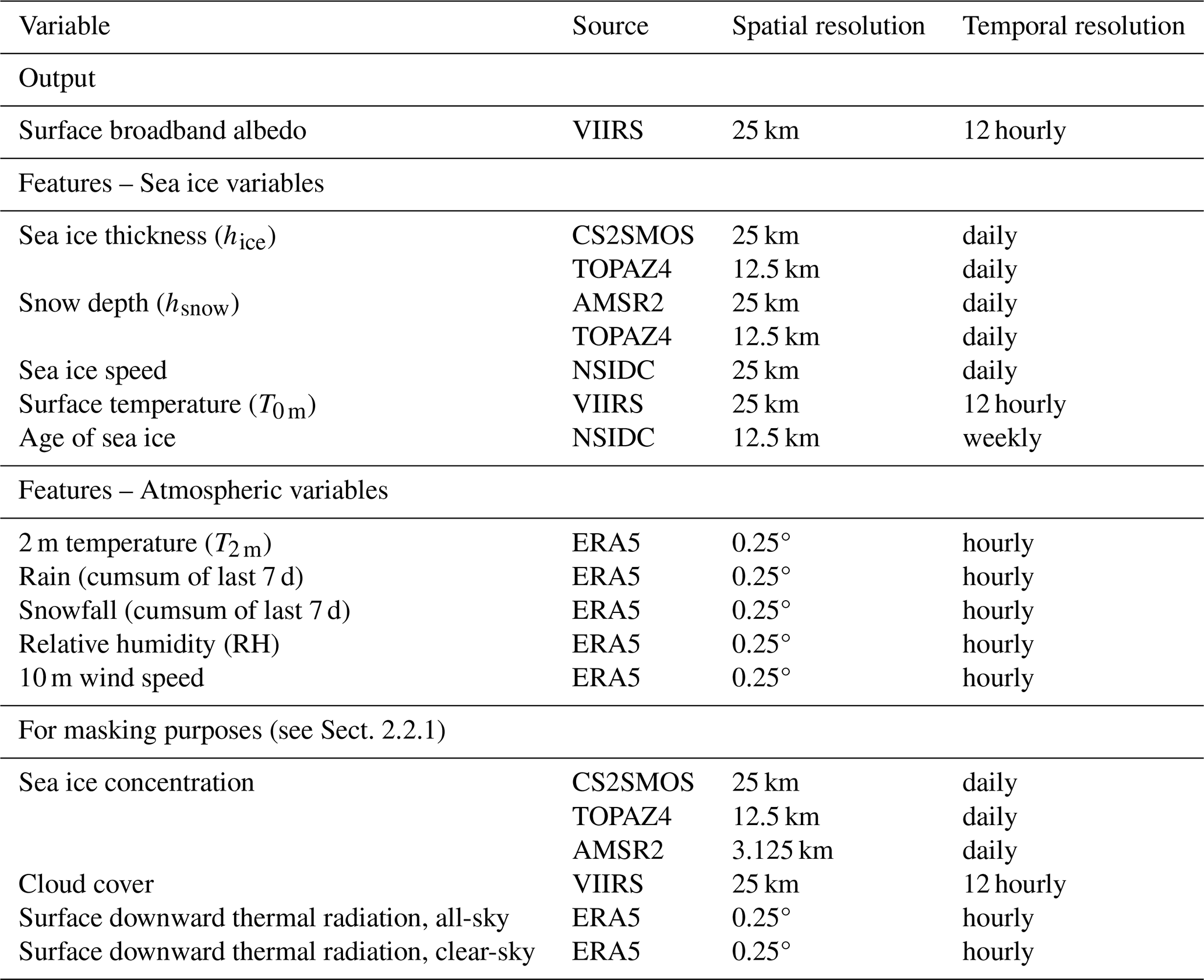
This study integrates multiple data products from satellites and reanalyses listed in Table 1, which we carefully select to ensure high-quality coverage of the entire pan-Arctic region on a daily basis. By intersecting the temporal and spatial domains of the data products, the overlapping period is from 2013–2020, during the months of March to September when sunlight is present in the whole pan-Arctic region. The final dataset consists of five sea ice and five atmospheric input features. For better readability, we refer to input features as features.

Table 1 Description of variables used in this study. Reanalysis data products are italised. The final dataset covers the years 2013–2020 as this is the period where the temporal coverages of all data products coincide.

2.1.1 Satellite data

The Polar Pathfinder – Extended Climate Data Record (CDR) product (Key et al., 2016, 2001) includes broadband albedo, surface temperature (T_0 m), and binary cloud mask (clear-sky/cloudy) with a temporal resolution of 12 h and a spatial resolution of 25 km. From 2013 until 2020, measurements are taken from the Visible Infrared Imaging Radiometer Suite (VIIRS). Compared with the SHEBA data, the albedo shows an uncertainty of about 7 % (Key et al., 2001).

The Level 4 SMOS-CryoSat (CS2SMOS) merged product (Ricker et al., 2017) includes daily sea ice thickness (h_ice) and sea ice concentration on a 25 km grid for March and April. The uncertainty, ranging from 0.1–0.5 m, is due to measurement inaccuracies and merging algorithms compared to airborne electromagnetic measurements.

The Advanced Microwave Scanning Radiometer 2 (AMSR2) satellite instrument provides daily snow depth data (h_snow) for March and April (Rostosky et al., 2018) and sea ice concentration data for the whole year (Spreen et al., 2008). Snow depth has a spatial resolution of 25 km, whereas sea ice concentration has a finer spatial resolution of 3.125 km. The uncertainty of snow depth is larger with increasing thickness, and slightly higher over multiyear ice than first year ice. Moreover, wrongly retrieved negative snow depth can occur over thin ice due to the signal coming from the ocean water. For sea ice concentrations below 65 %, the uncertainty in measurements reaches a maximum of 25 %, whereas at higher sea ice concentrations, the uncertainty is reduced to less than 10 %. These uncertainties stem from instrument-related errors, variability in atmospheric and surface conditions, and sensitivity of the algorithm to independent measurement validation.

The Polar Pathfinder Daily 25 km EASE-Grid Sea Ice Motion Vectors (Version 4) product (Tschudi et al., 2019a), which integrates data from various observations and reanalyses, gives sea ice velocity information. The EASE-Grid Sea Ice Age (Version 4) product (Tschudi et al., 2019b), with a spatial resolution of 12.5 km, provides weekly sea ice age with a temporal resolution of a year, meaning that an age of one indicates that the sea ice is up to one year old.

2.1.2 Reanalyses data

Satellite-based data for sea ice and snow depth are confined to the winter months (October/November–March/April) due to the limitations of satellite retrieval methods arising from the presence of melt ponds in summer (Ricker et al., 2017; Rostosky et al., 2018). To fill the gaps in the summer months (May–September), we use daily data of snow depth, sea ice thickness, and sea ice concentration from the Arctic Ocean Physics Reanalysis TOPAZ4b (European Union-Copernicus Marine Service, 2020). We deem it reasonable to use reanalysis data to fill the gaps as the correlation matrices of the satellite and reanalysis data are comparable for March and April (see Appendix A1). TOPAZ4b operates at a 12.5 km spatial resolution available from 1991–2023, based on the HYCOM ocean model (Bleck, 2002) coupled to a zero-layer scheme (Parkinson and Washington, 1979) with the elastic-viscous-plastic (EVP) rheology (Hunke and Dukowicz, 1997). ERA5 reanalysis data is used as forcing at the ocean surface. Sea ice concentration is assimilated with OSI-SAF (European Union-Copernicus Marine Service, 2015), while sea ice thickness data is assimilated with CS2SMOS. The Quality Information Document (Xie and Bertino, 2023) and the Synthesis Quality Overview (Bertino and Xie, 2023) of TOPAZ4b report that sea ice concentration on the sea ice edges retreats too rapidly in early summer and refreezes too fast in early winter compared to observations, with the thicker sea ice being underestimated. Snow depth is also underestimated, noticeably in June. From the ERA5 reanalysis product (Copernicus Climate Change Service, 2018a, b), we acquire hourly atmospheric surface data on a regular 0.25° longitude/latitude grid: 2 m temperature (T_2 m), rain, snowfall, relative humidity (RH), and 10 m wind speed, and surface downward thermal radiation under all-sky and clear-sky conditions.

2.2 Methods

Building on the principles outlined by Beucler et al. (2025) and Grundner et al. (2024), this study employs a Pareto optimality-based workflow as illustrated in Fig. 1.

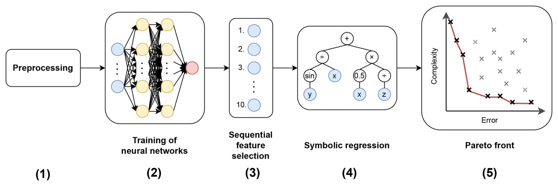
Figure 1 Pareto optimality-based workflow based on Beucler et al. (2025) and Grundner et al. (2024), exemplarily for discovering equations with symbolic regression. The process involves: (1) preprocessing of observational and reanalyses data to ensure consistency for the machine learning workflow, (2) training of multilayer perceptron neural networks (NNs), (3) sequential feature selection (SFS) for dimensionality reduction and identification of key features out of ten features governing sea ice albedo, (4) symbolic regression as data-driven equation discovery approach, and (5) comparison between the best-performing equations and baseline models (polynomials and NNs with reduced feature sets chosen by the SFS algorithm) on an error-complexity plane to evaluate how increasing model complexity reduces error.

2.2.1 Data preparation

This section describes the efforts taken to reconcile the different datasets from Sect. 2.1 and to illustrate the combined regional and temporal coverage. Using xESMF (Zhuang et al., 2024), remapping all data products (Table 1) to a common daily frequency on the albedo grid as reference grid ensures consistency and reliability of the final dataset and little modification of the albedo values as albedo is our target variable.

For albedo, we rely exclusively on daytime data due to its higher accuracy compared to nighttime data. To increase the sampling frequency of the weekly sea ice age data, we address gaps by applying the age value of the week's first day across the subsequent days. For ERA5 data, we calculate daily means for T_2 m, RH, 10 m wind speed, and surface downward thermal radiation under clear-sky and all-sky atmospheric conditions. Additionally, we adjust rain and snowfall data using a cumulative sum from the preceding seven days to consider a weekly memory effect. This cumulative sum is computed using an Eulerian framework and so neglects the potential influence of sea ice advection. This could modify the influence of these fields on the albedo state. We acknowledge that some of our predictor fields could be considered at different time lags and that other variables not considered here could influence surface albedo. However, we have retained the existing set of variables as a reasonable balance between completeness and feasibility. When transitioning from finer to a coarser grid, which is the case for TOPAZ4, NSIDC, ERA5 data, and AMSR2 for sea ice concentration, we employ a conservative regridder that maintains the integral of the source field by computing a weighted area mean over intersecting grids. For h_ice, h_snow, sea ice speed and concentration from CS2SMOS, bilinear regridding is sufficient for smoothly varying variables which match the resolution of the target grid.

Furthermore, we perform two masking operations to ensure equivalent atmospheric conditions and consistent spatial coverage across both observational and reanalyses products: cloud and sea ice pack masking. In terms of cloud masking, we use data samples where cloud conditions match across all data products, discarding the transition zone between clear-sky and cloudy conditions as cloud cover in the VIIRS product is a binary variable, only distinguishing between clear-sky and cloudy conditions. Since the total cloud cover variable in ERA5 is known to be overestimated in the Arctic region, Zampieri et al. (2023) proposed to compute the difference in surface downward thermal radiation between clear-sky and all-sky atmospheric conditions Δ_STRD to determine cloud conditions. Zampieri et al. (2023) defined ${\mathrm{\Delta }}_{\text{STRD}}\le \mathrm{15}\mathrm{W}{\mathrm{m}}^{-\mathrm{2}}$ to be clear-sky, $\mathrm{15}\mathrm{W}{\mathrm{m}}^{-\mathrm{2}}<{\mathrm{\Delta }}_{\text{STRD}}\le \mathrm{40}\mathrm{W}{\mathrm{m}}^{-\mathrm{2}}$ as the transition zone and ${\mathrm{\Delta }}_{\text{STRD}}>\mathrm{40}\mathrm{W}{\mathrm{m}}^{-\mathrm{2}}$ as cloudy. In addition, we only consider data samples where the sea ice concentration exceeds 80 %, defining a sea ice pack, with the aim to isolate the effects of the sea ice surface without the influence of ocean water. To omit adjacency effects such as land contamination, we perform a land mask with a buffer of 50 km. Figure 2 shows the number of data samples per month and Arctic subregion defined by Meier and Stewart (2023). In total, the final dataset consists of 7 903 463 data samples, with the Central Arctic being the most dominant region with 5 060 064 data samples.

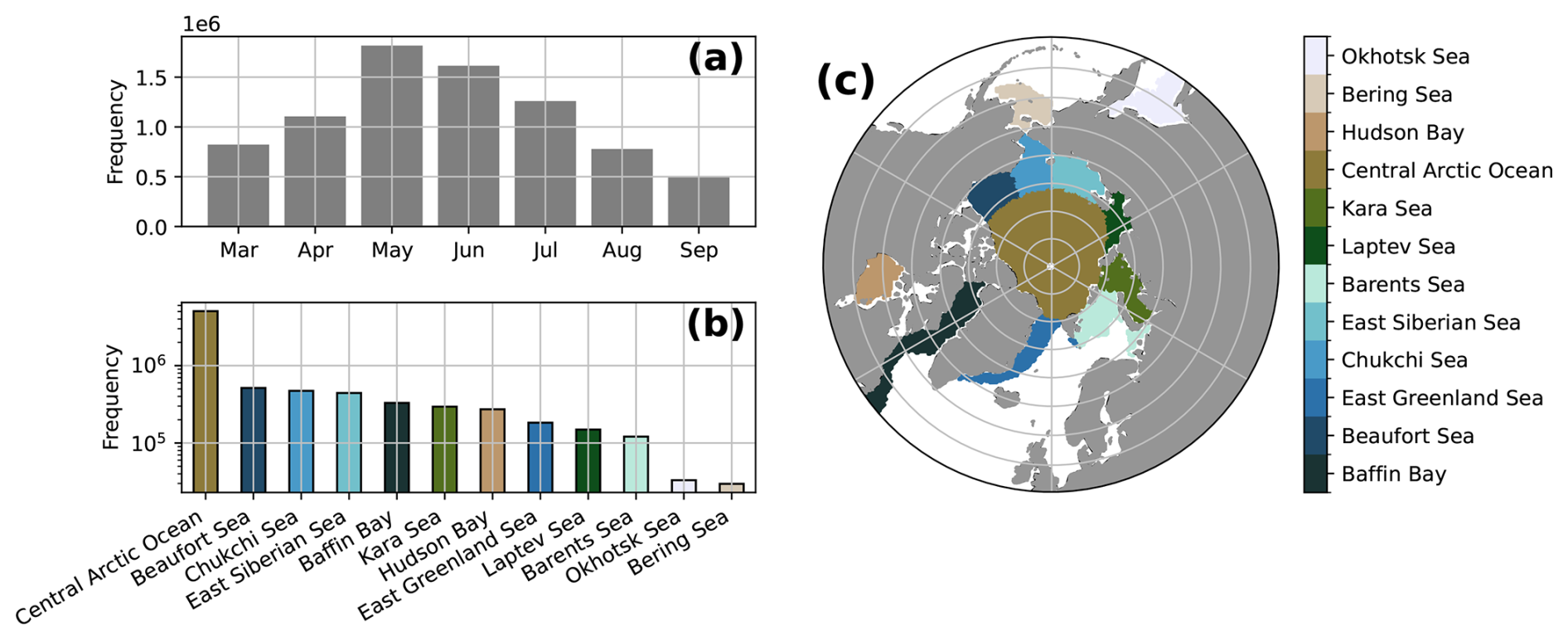
Figure 2 Panel (a) shows the monthly (March–September) and panel (b) the regional distribution of preprocessed dataset on a logarithmic y-axis with panel (c) illustrating the Arcitic subregions defined by Meier and Stewart (2023).

Let X be an m×n matrix representing the dataset, where m is the number of features, n is the number of samples and $\mathit{\sigma }=({\mathit{\sigma }}_{\mathrm{1}},{\mathit{\sigma }}_{\mathrm{2}},\mathrm{\dots },{\mathit{\sigma }}_m)\in {\mathbb{R}}^m$ is the vector of standard deviations for each feature. For our machine learning workflow, we split the dataset temporally into a training (2013–2018) and validation set (2019–2020) and standardise each sample X_j∈ℝ^m by dividing the feature values x_i,j by the corresponding standard deviation σ_i of the training set, yielding

$$\begin{array}{}\text{(1)}& {\mathbf{Z}}_j={\displaystyle \frac{{\mathbf{X}}_j}{\mathit{\sigma }}}=\left({\displaystyle \frac{x_{\mathrm{1},j}}{{\mathit{\sigma }}_{\mathrm{1}}}},{\displaystyle \frac{x_{\mathrm{2},j}}{{\mathit{\sigma }}_{\mathrm{2}}}},\mathrm{\dots },{\displaystyle \frac{x_{m,j}}{{\mathit{\sigma }}_m}}\right).\end{array}$$

Z is the resulting m×n standardised dataset matrix, with standardised samples Z_j∈ℝ^m. By this, we avoid preferential treatment of features that natively assume larger values.

2.2.2 Neural network architecture

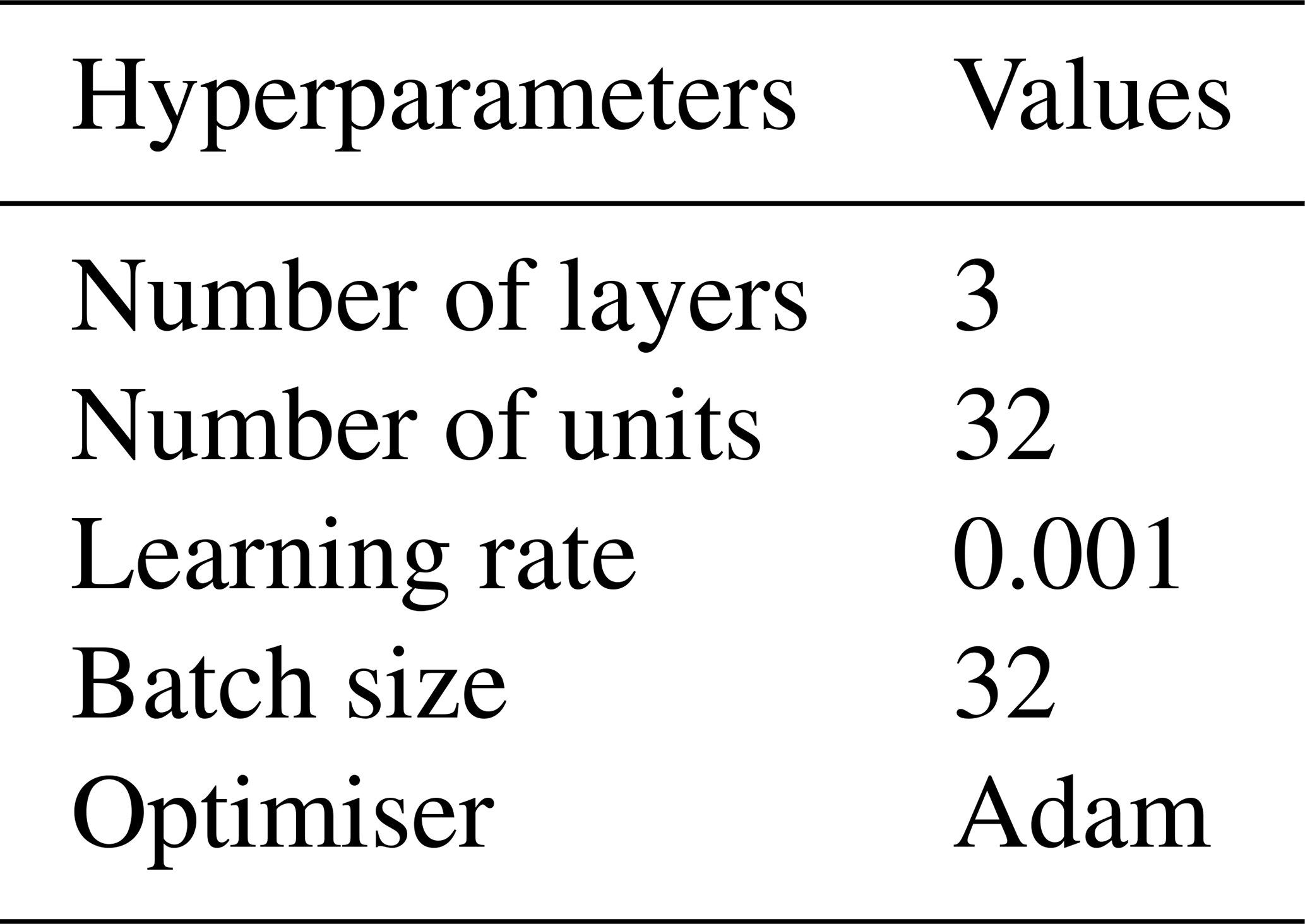
We train a multilayer perceptron NN using PyTorch (Paszke et al., 2019) by setting the hyperparameters to the default values in PyTorch and refining the number of layers, hidden units, learning rate, and batch size manually (Table 2). We fix Adam as the optimiser and the mean squared error (MSE) as the loss function, which measures the mean squared difference between the model prediction α(Z_j)∈ℝ (sea ice albedo) and the respective reference observation value y_j

$$\begin{array}{}\text{(2)}& \text{MSE}\stackrel{\text{def}}{=}{\displaystyle \frac{\mathrm{1}}{n}}\sum _{j=\mathrm{1}}^n\left(\mathit{\alpha }\right({\mathbf{Z}}_j)-y_j{)}^{\mathrm{2}}.\end{array}$$

Table 2 Hyperparameters of multilayer perceptron neural network using PyTorch (Paszke et al., 2019).

2.2.3 Sequential feature selection

Using the same NN architecture as described in Sect. 2.2.2, we use it as an estimator to perform forward SFS with SequentialFeatureSelector from the scikit-learn library (Pedregosa et al., 2011). SFS provides a ranking of feature importance which, in addition to helping us to maximise predictive performance using sparse models, can provide an intuition of the underlying physics. There are two reasons why we strive for reducing dimensionality: Symbolic regression performs best on low-dimensional data (see Sect. 2.2.4), and we seek parsimonious models, i.e. models that depend on few features to lower the model complexity and improve interpretability. Forward SFS begins by training the optimised NN with one feature and evaluating its performance based on the MSE on the validation set. The feature leading to the lowest MSE on the validation set can be considered to be the most informative from the set of features considered. In the following iterations, additional features are incorporated sequentially, retaining those that minimise the MSE. To reduce computational resources while still preserving robust results, we create ten subsets from the whole dataset with 10⁵ data samples each and perform SFS on each subset. To retrieve the overall ranking of the features, we average the ranking of each feature across all subsets.

2.2.4 Symbolic regression

Symbolic regression fits equations to the dataset, searching through the space of mathematical expressions based on predefined mathematical operators $(+,-,\sin ,\mathrm{\dots })$. Following Grundner et al. (2024), we use the PySR library by Cranmer et al. (2020) due to its flexibility and high success rate in benchmarking tests (De Franca et al., 2024). PySR is based on genetic programming and implements tree-based candidate solutions with tournament selection, local leaf search, and multiple populations, which is inherently stochastic. PySR's strength lies in the exploration of a large range of possible solutions, overcoming the potential issue to converge to suboptimal or overfit solutions as opposed to deterministic methods.

We find five features to be the practical upper bound which we retrieve from the ranking of our previous SFS results. Given that PySR is capable of discovering compact and interpretable equations of low complexity, it can operate effectively with a reduced dataset. Consequently, we randomly downsample the training set to 10 000 data samples, ensuring that the training set is representative for the entire dataset and leveraging the efficiency of PySR in handling limited data. We run PySR with varying hyperparameters to explore various symbolic forms that describe the data well, e.g. excluding trigonometric operators, exponents or logarithms. As there is no guarantee that the discovered equations are optimal for their complexity, we perform multiple runs, producing about 800 equations in total. We directly filter out equations with a storage size greater than 1500 bits to neglect long and complex equations.

To ensure physical consistency, the equations should satisfy the following physical constraints (PC): (1) The value of sea ice albedo α should be between 0 and 1; (2) snow depth h_snow significantly increases α (Grenfell and Maykut, 1977; Grenfell and Perovich, 2004); (3) under freezing conditions, thicker ice h_ice has a higher α than thinner ice (Perovich, 1996); (4) with rising surface temperature, sea ice melts, driving melt pond formation, which decreases α significantly (Grenfell and Maykut, 1977; Perovich, 1996); (5) the function should be smooth over the entire domain. The PCs are approximations which we assume for large-scale applications and for simplicity. We do not account for microstructural characteristics such as salinity and atmospheric aerosol deposition. For instance, younger, bare ice typically has higher salinity, which may increase scattering and therefore increase albedo comparable to multiyear ice (Light et al., 2015; Perovich and Grenfell, 1981), while deposition of atmospheric aerosols reduces albedo independent of snow or sea ice thickness (e.g. Warren and Wiscombe, 1980; Hansen and Nazarenko, 2004). We can mathematically formalise these PCs for all samples Z_j

$$\begin{array}{rl}{\displaystyle }\text{PC1}:& {\displaystyle }\mathit{\alpha }\left({\mathbf{X}}_j\right)\in [\mathrm{0},\mathrm{1}]\\ {\displaystyle }\text{PC2}:& {\displaystyle }\partial \mathit{\alpha }\left({\mathbf{X}}_j\right)/\partial h_{\text{snow}}\ge \mathrm{0}\\ {\displaystyle }\text{PC3}:& {\displaystyle }\partial \mathit{\alpha }\left({\mathbf{X}}_j\right)/\partial h_{\text{ice}}\ge \mathrm{0}\\ {\displaystyle }\text{PC4}:& {\displaystyle }\partial \mathit{\alpha }\left({\mathbf{X}}_j\right)/\partial T_{\mathrm{0}\mathrm{m}}\le \mathrm{0}\\ {\displaystyle }\text{PC5}:& {\displaystyle }\mathit{\alpha }\left({\mathbf{X}}_j\right)\text{ is a smooth function.}\end{array}$$

As some equations are too complex to be solved analytically, each equation α(X) is checked for these PCs by approximating the first-order partial derivative with respect to a feature x with the central difference method

$$\begin{array}{}\text{(3)}& {\displaystyle \frac{\partial \mathit{\alpha }}{\partial x}}\approx {\displaystyle \frac{\mathit{\alpha }(x+h)-\mathit{\alpha }(x-h)}{\mathrm{2}h}},\end{array}$$

where $h={\mathrm{10}}^{-\mathrm{5}}$ defines the step size for finite difference.

Keeping the physically consistent equations that satisfy all PCs, we perform a secondary optimisation on a randomly sampled subset of 10⁵ data samples from the training set. This involves introducing an additional coefficient for each feature in the equation, unless PySR has already generated it. The minimize function from the SciPy library (Virtanen et al., 2020) allows a robust framework for minimisation using the Nelder–Mead (Nelder and Mead, 1965) and Broyden–Fletcher–Goldfarb–Shanno (BFGS) methods (Nocedal and Wright, 2006), common choices for general nonlinear optimisation problems.

2.2.5 Pareto-optimal models

Having found the best-performing equations that satisfy the PCs, we compare the equations with baseline models within an error-complexity graph, illustrating the gain of increasing model complexity with respect to the error. The baseline models are polynomials of degree one to four using PolynomialFeatures from the Scikit-learn library (Pedregosa et al., 2011), and the trained NN from Sect. 2.2.2. Furthermore, we also include the parsimonious NN models from Sect. 2.2.3. Likewise, we perform SFS on the polynomials, analogous to how it is described in Sect. 2.2.3, and include them in the error-complexity graph. The measure of error is the MSE, while the model complexity is defined as the number of tunable parameters. Therefore, the model complexity can be increased in two ways: increasing the feature dimensionality and increasing the degree of a polynomial. For the NN architecture used in this study, adding one feature does not substantially increase the model complexity since adding one feature is equivalent to adding a single node in the NN.

3 Analysis of the best-performing equation

3.1 Feature importance in the baseline models

The numbers in brackets indicate the averaged ranking across the ten subsets. When no bracket is indicated, the ranking of a feature remains consistent across all subsets. Let 𝒫_d be a polynomial of degree $d\in \mathit{\{}\mathrm{1},\mathrm{2},\mathrm{3},\mathrm{4}\mathit{\}}$. The SFS algorithm reveals the following feature rankings for 𝒫₁₋₄ and NN:

$$\begin{array}{rl}{\displaystyle }{\mathcal{P}}_{\mathrm{1}}:& {\displaystyle }{h}_{\text{snow}}\to T_{\mathrm{0}\mathrm{m}}\to T_{\mathrm{2}\mathrm{m}}\to \text{rain}\to \text{snowfall}\to h_{\text{ice}}\\ {\displaystyle }& {\displaystyle }\to \text{RH}\to \text{wind speed}\to \text{ice speed}\to \text{age}\\ {\displaystyle }{\mathcal{P}}_{\mathrm{2}}:& {\displaystyle }{h}_{\text{snow}}\to T_{\mathrm{0}\mathrm{m}}\to h_{\text{ice}}\to T_{\mathrm{2}\mathrm{m}}\to \text{snowfall}\\ {\displaystyle }& {\displaystyle }\to \text{RH}\to \text{ice speed}\left(\mathrm{7.5}\right)\to \text{rain}\left(\mathrm{7.9}\right)\\ {\displaystyle }& {\displaystyle }\to \text{wind speed}\left(\mathrm{8.6}\right)\to \text{age}\\ {\displaystyle }{\mathcal{P}}_{\mathrm{3}}:& {\displaystyle }{h}_{\text{snow}}\to T_{\mathrm{0}\mathrm{m}}\to T_{\mathrm{2}\mathrm{m}}\to h_{\text{ice}}\to \text{snowfall}\\ {\displaystyle }& {\displaystyle }\to \text{RH}\to \text{age}\left(\mathrm{7.1}\right)\to \text{wind speed}\left(\mathrm{8.8}\right)\\ {\displaystyle }& {\displaystyle }\to \text{rain}\left(\mathrm{8.9}\right)\to \text{ice speed}\left(\mathrm{9.2}\right)\\ {\displaystyle }{\mathcal{P}}_{\mathrm{4}}:& {\displaystyle }{h}_{\text{snow}}\to T_{\mathrm{0}\mathrm{m}}\to h_{\text{ice}}\left(\mathrm{3.2}\right)\to T_{\mathrm{2}\mathrm{m}}\left(\mathrm{3.9}\right)\to \text{RH}\left(\mathrm{6.6}\right)\\ {\displaystyle }& {\displaystyle }\to \text{age}\left(\mathrm{6.8}\right)\to \text{wind speed}\left(\mathrm{7.4}\right)\to \text{snowfall}\left(\mathrm{7.6}\right)\\ {\displaystyle }& {\displaystyle }\to \text{ice speed}\left(\mathrm{8.2}\right)\to \text{rain}\left(\mathrm{8.4}\right)\\ {\displaystyle }\text{NN}:& {\displaystyle }{h}_{\text{snow}}\to T_{\mathrm{0}\mathrm{m}}\to h_{\text{ice}}\left(\mathrm{3.2}\right)\to T_{\mathrm{2}\mathrm{m}}\left(\mathrm{3.8}\right)\\ {\displaystyle }& {\displaystyle }\to \text{snowfall}\left(\mathrm{5.6}\right)\to \text{RH}\left(\mathrm{7.0}\right)\to \text{rain}\left(\mathrm{7.8}\right)\\ {\displaystyle }& {\displaystyle }\to \text{wind speed}\left(\mathrm{8.0}\right)\to \text{ice speed}\left(\mathrm{8.2}\right)\to \text{age}\left(\mathrm{8.4}\right)\end{array}$$

In all model families, there is a consistent pattern in the ranking of the most informative features. All model types identify h_snow as the most informative predictor and T_0 m as the second most informative predictor. h_snow being the most informative predictor is plausible since snow is among the most reflective medium in natural surfaces, especially when fresh and dry. When present, snow represents the uppermost layer where solar radiation initially impacts. Snow has a low optical depth due to the scattering of incoming solar radiation in diffusive directions, implying that a snow layer of a few centimeters significantly increases surface albedo (Grenfell and Maykut, 1977). Additionally, at the spatial scales of our dataset (25 km), snow depth is likely related to snow fractional coverage which is also impactful for albedo. T_0 m as the second most informative predictor is in agreement with the fact that T_0 m is a proxy of whether the surface is under melting or freezing conditions, as the presence of melting water reduces albedo. For instance, fresh snow exhibits a higher albedo compared to wet snow (Grenfell and Maykut, 1977). Sea ice albedo parametrisations that do not explicitly resolve melt ponds include the radiative effect of melt ponds implicitly with T_0 m (e.g. PW79). Excluding the linear model, the top predictors after h_snow and T_0 m are h_ice and T_2 m. As sea ice has a higher optical depth than snow, h_ice ranked below h_snow seems plausible, implying that h_snow provides larger marginal predictive improvement than h_ice.

The inclusion of T_2 m among the most informative predictors is unexpected given the high correlation (0.92) between T_0 m and T_2 m (see Appendix A2), which would suggest redundancy in T_2 m, ranked below T_0 m. Nevertheless, SFS quickly chooses T_2 m as an additional predictor after T_0 m is accounted for, indicating that α is not only dependent on surface conditions, but is also influenced by atmospheric conditions near the surface, affecting the optical properties of the sea ice surface. Additionally, this may be in part due to the fact that T_2 m can go above the melting point, whereas T_0 m cannot. Another consideration is that ERA5 does not assimilate sea ice or snow thickness, nor near-surface Arctic observations, except for surface pressure from stations and drifting buoys. Previous studies have shown that this leads to warm temperature biases in ERA5 over the Arctic, particularly during polar winter clear-sky events (Batrak and Müller, 2019; Zampieri et al., 2023). Such biases could introduce inconsistencies between the satellite-derived T_0 m and the ERA5-biased T_2 m , which might partly contribute to the predictive skill attributed to T_2 m. The documented warm bias is particularly large during polar winter stable boundary conditions. Our exclusive use of polar-day samples thus helps mitigate the influence of this bias. However, this documented warm bias in ERA5 and data inconsistencies between surface and 2 m air temperatures may play some role in our results, although we believe it is unlikely to fully explain the relationship identified here. To the best of our knowledge, existing sea ice albedo parametrisations in ESMs with an implicit scheme of melt pond representation do not include T_2 m. Sea ice models that explicitly resolve melt ponds, e.g. Flocco et al. (2010) and Hunke et al. (2013), use T_2 m to compute the surface melting rate to calculate the melt water accumulation in the ponds.

In implicit schemes, the transition of T_0 m around the freezing point of sea ice is used as information to implicitly determine melting and freezing conditions, which characterise the wetness of sea ice surface, altering sea ice optical properties. Examining in-situ measurements of T_2 m from the MOSAiC expedition and satellite swath data of melt pond fraction with a resolution of 1.2 km, Niehaus et al. (2025) have reported that T_2 m is one of the main driver of the formation and evolution of melt ponds, explaining short-lived changes in melt pond fractions and thus, decreasing albedo. Although they concluded that ERA5 reanalysis data are not well suited to study local melt pond characteristics due to the coarse spatial resolution, here we show that T_2 m of ERA5 is a valuable predictor to understand the large-scale mechanisms that modulate sea ice albedo in the pan-Arctic region.

The ranking of the remaining features shows some variability across model families, but some patterns can be identified. For instance, snowfall and RH tend to be ranked higher than wind speed, ice speed, and age in most model families. On a large scale, features related to thermodynamics are more relevant to describe sea ice albedo than features related to sea ice motion.

3.2 Physical interpretation of the best-performing equation

PySR selects the four best ranking features chosen by the SFS algorithm for the NN (see Sect. 3.1), namely h_snow, T_0 m, h_ice, and T_2 m, and neglects snowfall. This results in the following physically consistent equation with the lowest MSE

$$\begin{array}{}\text{(4)}& \begin{array}{rl}{\displaystyle }& {\displaystyle }\mathit{\alpha }\left(h_{\text{snow}},h_{\text{ice}},T_{\mathrm{2}\mathrm{m}},T_{\mathrm{0}\mathrm{m}}\right)=\\ {\displaystyle }& {\displaystyle }{\displaystyle \frac{{\tanh }^{\mathrm{2}}({\stackrel{\mathrm{̃}}{p}}_{\text{snow}}{h}_{\text{snow}}^{\mathrm{2}}+{\stackrel{\mathrm{̃}}{p}}_{\text{ice}}{h}_{\text{ice}}+\stackrel{\mathrm{̃}}{a})}{\stackrel{\mathrm{̃}}{b}-\tanh ({\stackrel{\mathrm{̃}}{p}}_{T_{\mathrm{2}\mathrm{m}}}{T}_{\mathrm{2}\mathrm{m}}-{\stackrel{\mathrm{̃}}{p}}_{T_{\mathrm{0}\mathrm{m}}}{T}_{\mathrm{0}\mathrm{m}}+\stackrel{\mathrm{̃}}{c})}}.\end{array}\end{array}$$

Equation (4) contains seven coefficients for which the optimised values are as follows

$$\begin{array}{rl}{\displaystyle }& {\displaystyle }\mathit{\{}{\stackrel{\mathrm{̃}}{p}}_{\text{snow}},{\stackrel{\mathrm{̃}}{p}}_{\text{ice}},{\stackrel{\mathrm{̃}}{p}}_{T_{\mathrm{2}\mathrm{m}}},{\stackrel{\mathrm{̃}}{p}}_{T_{\mathrm{0}\mathrm{m}}},\stackrel{\mathrm{̃}}{a},\stackrel{\mathrm{̃}}{b},\stackrel{\mathrm{̃}}{c}\mathit{\}}=\\ {\displaystyle }& {\displaystyle }\left\{\mathrm{63.13}{\displaystyle \frac{\mathrm{1}}{{\text{m}}^{\mathrm{2}}}},\mathrm{0.11}{\displaystyle \frac{\mathrm{1}}{\text{m}}},\mathrm{0.14}{\displaystyle \frac{\mathrm{1}}{\mathrm{°}\mathrm{C}}},\mathrm{0.30}{\displaystyle \frac{\mathrm{1}}{\mathrm{°}\mathrm{C}}},\mathrm{0.84},\mathrm{2.19},\mathrm{0.95}\right\},\end{array}$$

where ${\stackrel{\mathrm{̃}}{p}}_x$ denotes the weight of a feature x. The following Sections highlight the main physical findings discovered by Eq. (4) and which role the coefficients play.

3.2.1 High sensitivity to small variations in thin snow

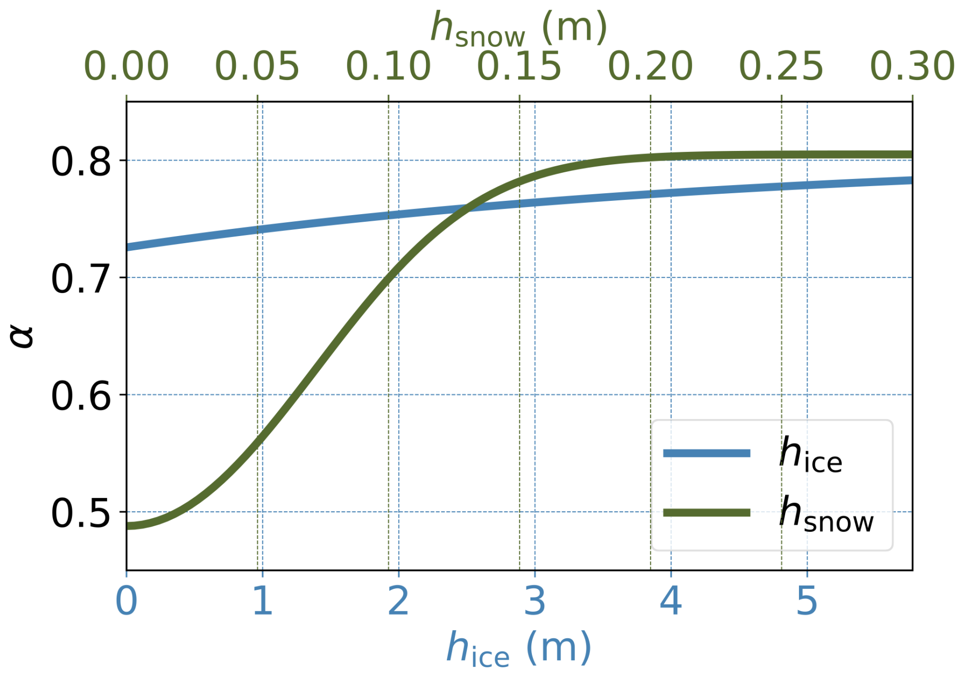
In the numerator of Eq. (4), the squared hyperbolic tangent asymptotically approaches 1, causing changes in h_snow to have a greater impact on α than changes in h_ice for smaller values. For x→0 we have

$$\begin{array}{}\text{(5)}& \tanh \left(x\right)=x+O\left(x^{\mathrm{3}}\right)\end{array}$$

due to Taylor's theorem. Squaring Eq. (5) yields

$$\begin{array}{}\text{(6)}& \begin{array}{rl}{\displaystyle }& {\displaystyle }{\tanh }^{\mathrm{2}}\left({\stackrel{\mathrm{̃}}{p}}_{\text{snow}}{h}_{\text{snow}}^{\mathrm{2}}+{\stackrel{\mathrm{̃}}{p}}_{\text{ice}}{h}_{\text{ice}}+\stackrel{\mathrm{̃}}{a}\right)\approx \\ {\displaystyle }& {\displaystyle }{\left({\stackrel{\mathrm{̃}}{p}}_{\text{snow}}{h}_{\text{snow}}^{\mathrm{2}}+{\stackrel{\mathrm{̃}}{p}}_{\text{ice}}{h}_{\text{ice}}+\stackrel{\mathrm{̃}}{a}\right)}^{\mathrm{2}}\end{array}\end{array}$$

for small values. As h_snow and h_ice increase, their impact on α diminishes due to the asymptotic nature of the hyperbolic tangent. Figure 3 illustrates how α changes rapidly within the first 20 cm of snow and then approaches an upper limit, whereas the relationship with h_ice is approximately linear with a small rate of change. The rapid increase of α within the first centimetres of snow aligns with known sea ice physics, as surface albedo is highly sensitive to small changes in thin snow, but becomes insensitive to differences in thicker snow and sea ice (e.g. Grenfell and Maykut, 1977; Perovich, 1996). Conversely, Perovich (1996) showed in a laboratory experiment that sea ice albedo also behaves asymptotically with increasing sea ice thickness. Here, due to the low weight value of h_ice, there is little difference in α response when increasing h_ice.

Figure 3 The response of Eq. (4) to varying snow depth (h_snow) and sea ice thickness (h_ice). While varying snow depth h_snow or sea ice thickness h_ice, the other features are fixed to their mean values during the validation period (2019–2020), shown in Table B1 (see Appendix B).

3.2.2 The weighted difference between the surface and 2 m air temperature as a seasonal proxy

Let ΔT^* be the weighted temperature difference that incorporates the weights:

$$\begin{array}{}\text{(7)}& \mathrm{\Delta }{T}^{*}={\stackrel{\mathrm{̃}}{p}}_{T_{\mathrm{2}\mathrm{m}}}{T}_{\mathrm{2}\mathrm{m}}-{\stackrel{\mathrm{̃}}{p}}_{T_{\mathrm{0}\mathrm{m}}}{T}_{\mathrm{0}\mathrm{m}}\end{array}$$

PySR highlights that ΔT^* is more critical than the individual temperatures, with T_0 m having double the impact on the denominator's hyperbolic tangent function in Eq. (4) compared to T_2 m, according to their weights. This supports the feature importance ranking (see Sect. 3.1), where T_0 m is ranked higher than T_2 m, while both rank among the top four features despite their strong linear correlation of 0.92 (see Appendix A2). Although T_0 m holds more weight than T_2 m, their importance remains interlinked due to this correlation, making their joint behaviour informative.

The hyperbolic tangent function in the denominator is strictly monotonically increasing, ranging between −1 and 1, approaching −1 as its input tends to negative infinity and 1 as it tends to positive infinity. Up to a constant, the ΔT^* controls both the sign and the magnitude in the argument of tanh. Assuming ${\stackrel{\mathrm{̃}}{p}}_{T_{\mathrm{2}\mathrm{m}}}$ and ${\stackrel{\mathrm{̃}}{p}}_{T_{\mathrm{0}\mathrm{m}}}$ are always positive, if ΔT^* is positive, tanh (ΔT^*) is pushed towards 1 and increases the overall value of $\mathit{\alpha }(h_{\text{snow}},h_{\text{ice}},T_{\mathrm{2}\mathrm{m}},T_{\mathrm{0}\mathrm{m}})$. If ΔT^* is negative, tanh (ΔT^*) is shifted towards -1, decreasing the overall value of $\mathit{\alpha }(h_{\text{snow}},h_{\text{ice}},T_{\mathrm{2}\mathrm{m}},T_{\mathrm{0}\mathrm{m}})$.

Figure 4a and b illustrate how transforming the temperature difference $\mathrm{\Delta }T=T_{\mathrm{2}\mathrm{m}}-T_{\mathrm{0}\mathrm{m}}$ to ΔT^* elucidates its relationship with observed sea ice albedo. At higher ΔT^*, α consistently remains high (α=0.85), unlike ΔT, where high α occurs between −15 and 15°C. Notably, when ΔT^* approaches zero, α decreases rapidly, an aspect which is not obvious with ΔT. Plotting the seasonal cycle in Fig. 4c, ΔT^* decreases steadily from winter, reaching a minimum of -0.19 in mid-July and then increases towards the fall, while ΔT shows two cycles with minima in May and mid-July. Consequently, ΔT^* serves as a seasonal proxy, where high ΔT^* corresponds to winter, early spring, and autumn, implying freezing and freeze-up conditions, whereas low ΔT^* aligns with late spring and summer, indicating melting conditions. The combined information of the sea ice surface and atmospheric conditions in ΔT^* can be interpreted as indicator for the transition between freezing and melting conditions.

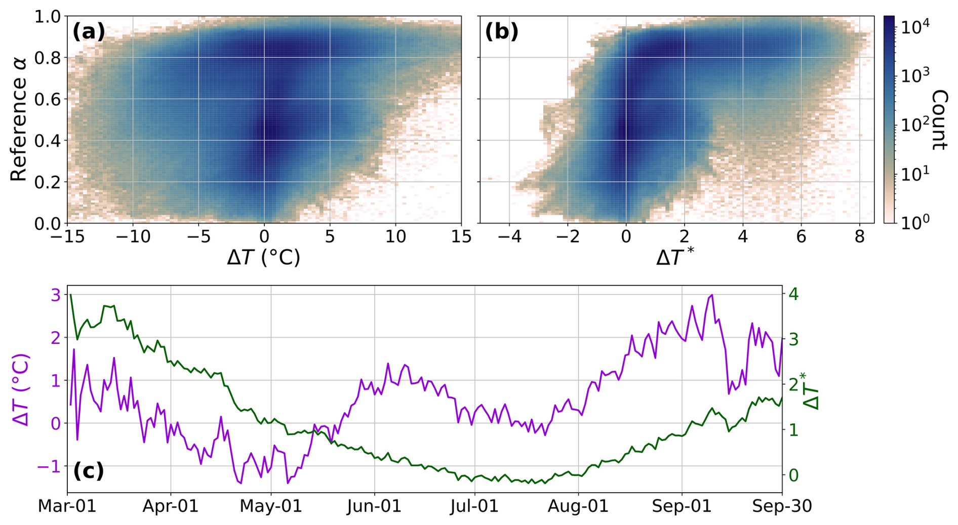
Figure 4 Comparison between the temperature difference $\mathrm{\Delta }T=T_{\mathrm{2}\mathrm{m}}-T_{\mathrm{0}\mathrm{m}}$ and the weighted temperature difference $\mathrm{\Delta }{T}^{*}=\stackrel{\mathrm{̃}}{p_{T_{\mathrm{2}\mathrm{m}}}}{T}_{\mathrm{2}\mathrm{m}}-\stackrel{\mathrm{̃}}{p_{T_{\mathrm{0}\mathrm{m}}}}{T}_{\mathrm{0}\mathrm{m}}$. Panels (a) and (b) show the density heat map for the observed sea ice albedo α and ΔT and ΔT^*, respectively, on a logarithmic scale. Panel (c) illustrates the seasonal cycle of observed ΔT and ΔT^* from 1 March–30 September averaged from 2013 until 2020.

Since tanh (x) asymptotically approaches −1 and 1, the function becomes insensitive to large temperature differences, which is consistent with physical expectations, since extreme temperature differences do not significantly affect albedo once the ice is either fully melted or frozen.

While we expect that ΔT^* is providing meaningful physical information, the seasonal cycle that is reflected in ΔT^* could be influenced by the aforementioned bias in ERA5 T_2 m which is the largest during the cold season and not present during summer months. Nevertheless, it does suggest that information on the seasonal cycle is useful in providing a constraint on the surface albedo. Other possible predictors that encode information on the seasonal cycle, such as solar insolation or the surface energy balance, could also provide useful information and could be explored in future work. Considerations of training data biases and prioritisation of predictors that enable results to be generalised across regions and different climate states are important for possible ML-based parametrisations that could be developed based on this work.

3.2.3 Control of the upper and lower limit of sea ice albedo and the transition between melting and freezing conditions

In the following, we analyse the impact of the coefficients $\stackrel{\mathrm{̃}}{a}$, $\stackrel{\mathrm{̃}}{b}$ and $\stackrel{\mathrm{̃}}{c}$ on the sea ice albedo predictions. Equation (4) approaches its infimum (α_inf) when snow and ice are not present and when the denominator is maximised

$$\begin{array}{}\text{(8)}& {\mathit{\alpha }}_{\text{inf}}={\displaystyle \frac{{\tanh }^{\mathrm{2}}\left(\stackrel{\mathrm{̃}}{a}\right)}{\stackrel{\mathrm{̃}}{b}+\mathrm{1}}}\text{for}\stackrel{\mathrm{̃}}{b}>-\mathrm{1}.\end{array}$$

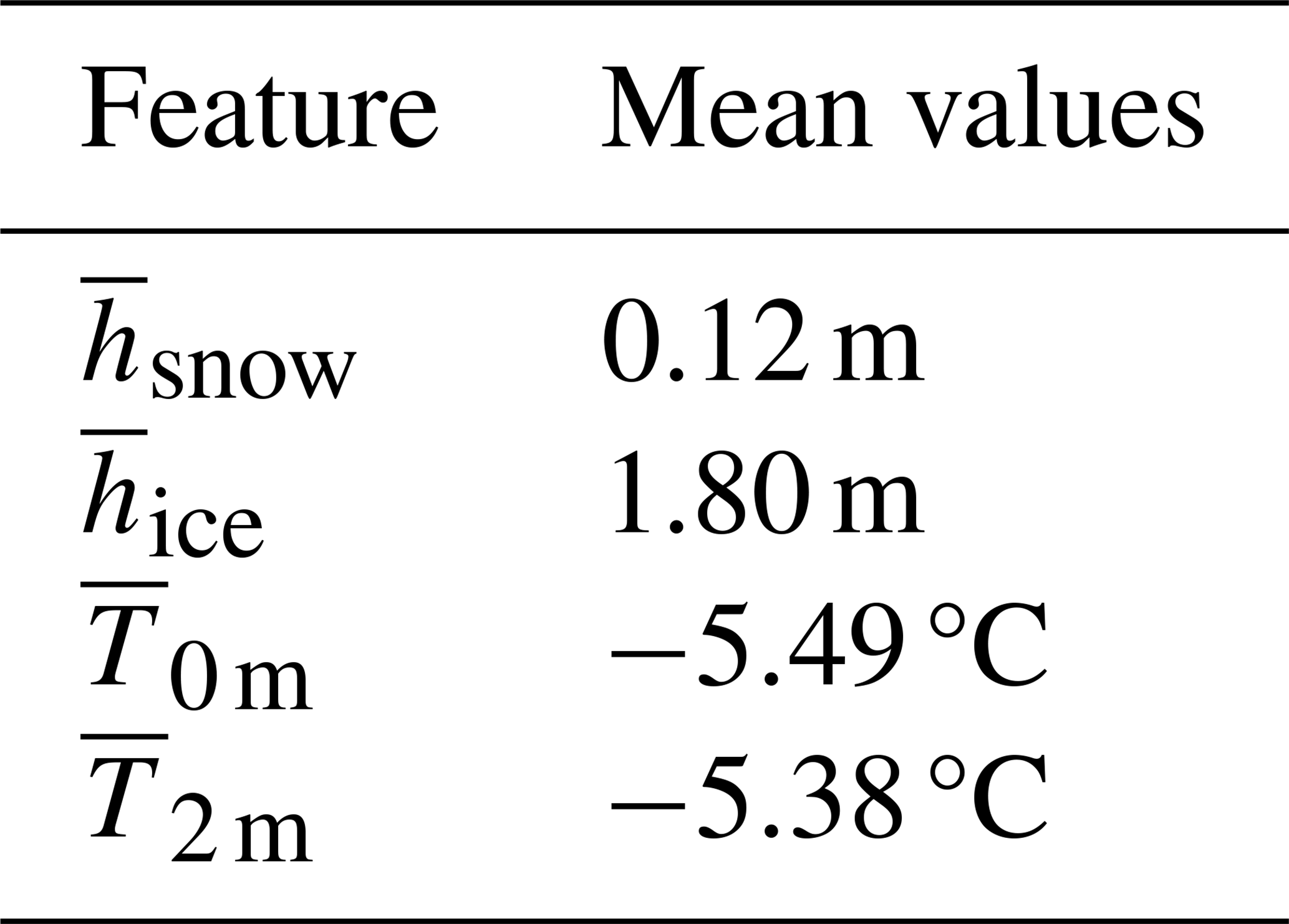
Equation (8) highlights that $\stackrel{\mathrm{̃}}{a}$ controls the lower limit of α, as depicted in Fig. 5a, which examines how α depends on h_snow with different $\stackrel{\mathrm{̃}}{a}$ values, while other features are set to their mean during validation (Table B1 in Appendix B). The analysis focuses solely on h_snow due to its greater influence on α compared to h_ice (see Sect. 3.2.1). The coefficient $\stackrel{\mathrm{̃}}{a}$ controls how quickly ${\tanh }^{\mathrm{2}}(h_{\text{snow}}^{\mathrm{2}}+h_{\text{ice}})$ grows from its lower limit, as increasing $\stackrel{\mathrm{̃}}{a}$ shifts $h_{\text{snow}}^{\mathrm{2}}+h_{\text{ice}}+\stackrel{\mathrm{̃}}{a}$ to the right, making ${\tanh }^{\mathrm{2}}(h_{\text{snow}}^{\mathrm{2}}+h_{\text{ice}}+\stackrel{\mathrm{̃}}{a})$ reach higher values more quickly. So, increasing $\stackrel{\mathrm{̃}}{a}$ raises the lower limit and makes the function grow faster from its minimum.

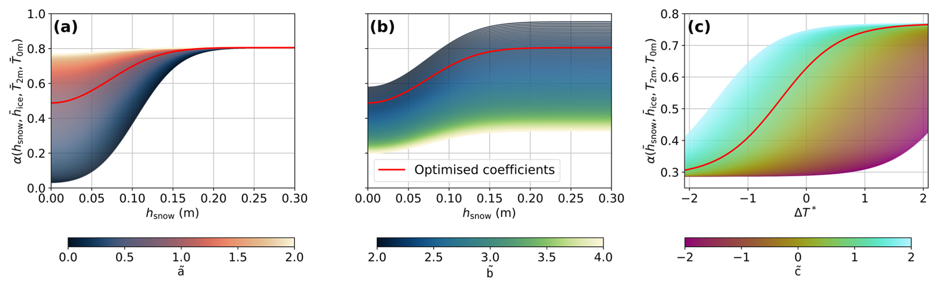
Figure 5 The impact of the coefficients $\stackrel{\mathrm{̃}}{a}$, $\stackrel{\mathrm{̃}}{b}$ and $\stackrel{\mathrm{̃}}{c}$ on the functional behaviour of Eq. (4). Panels (a) and (b) illustrate the dependency of sea ice albedo (α) on snow depth (h_snow) with varying $\stackrel{\mathrm{̃}}{a}$ and $\stackrel{\mathrm{̃}}{b}$, respectively. Panel (c) demonstrates the response on the difference between 2 m temperature (T_2 m) and surface temperature (T_0 m) with varying $\stackrel{\mathrm{̃}}{c}$. The other coefficients are kept fixed at their optimal values and the other features at their mean values during the validation period (2019–2020) denoted with bar overhead (Table B1 in Appendix B). The red line indicates Eq. (4) with the optimised coefficient values (see Sect. 3.2).

Equation (4) approaches its supremum (α_sup) when the numerator is maximised and the denominator is minimised, while $\stackrel{\mathrm{̃}}{b}$ is controlling the upper limit of α

$$\begin{array}{}\text{(9)}& {\mathit{\alpha }}_{\text{sup}}={\displaystyle \frac{\mathrm{1}}{\stackrel{\mathrm{̃}}{b}-\mathrm{1}}}\text{for}\stackrel{\mathrm{̃}}{b}>\mathrm{1}.\end{array}$$

As $\stackrel{\mathrm{̃}}{b}$ increases, the upper limit decreases and vice versa (Fig. 5b). Since the denominator must be greater than 1 to keep α within its physical range (0–1), $\stackrel{\mathrm{̃}}{b}$ should be greater than 2 to ensure physical consistency. Plugging in the optimised coefficients, we get α_inf=0.15 and α_sup=0.84.

The coefficient $\stackrel{\mathrm{̃}}{c}$ shifts the response curve of Eq. (4), thereby modulating the transition between freezing and melting conditions (Fig. 5c). Decreasing $\stackrel{\mathrm{̃}}{c}$ shifts the response curve to the right, meaning that melting conditions already occur at higher ΔT^*, and vice versa, suggesting the presence of other sources (e.g., oceanic heat) influencing sea ice optical properties, which are not accounted for in Eq. (4).

4 Comparison of Eq. (4) with PW79 and baseline models

4.1 Balancing model error and complexity

Figure 6 presents the five best-performing equations in terms of MSE discovered by PySR (see Appendix C for the equations ranked second to fifth with the respective PySR configurations) and baseline models, including polynomials and NNs, on an error-complexity plane (see Sect. 2.2.5). Optimising PW79 using the Nelder–Mead method reduces the MSE from 0.08–0.03. Despite this improvement, all models outperform the tuned PW79.

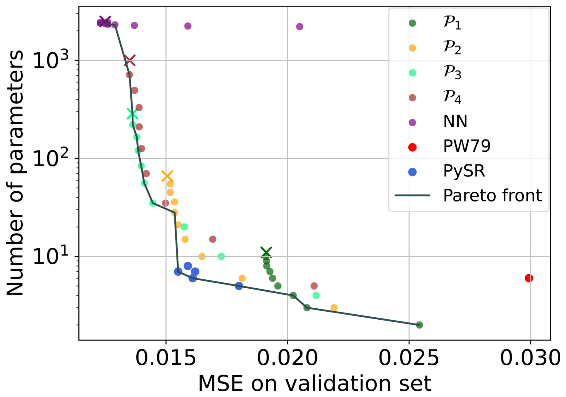
Figure 6 Error-complexity plane. The mean squared error (MSE) on the validation set is on the x-axis, while model complexity, defined as the number of tunable parameters, is plotted on a logarithmic y-axis. We compare the five best-performing physically consistent equations derived with PySR with the tuned Parkinson and Washington (1979, PW79) parametrisation and with baseline models of different types: polynomials of different degrees 𝒫₁₋₄, and neural networks (NNs). For each model type, models with an increasing number of features, chosen by the sequential feature selection (SFS) algorithm, are evaluated. With the exception of the NNs, those can be read from right to left with increasing number of features. Models with all ten features are marked with a cross. The Pareto front traces out the best models for a given maximum complexity.

Notably, increasing the polynomial degree from one to two yields a significant reduction in MSE of approximately 0.005. However, further increasing the degree to three or four does not result in substantial performance gains, indicating that model complexity beyond this point does not lead to significant improvements. Moreover, increasing feature dimensionality leads to a convergence of model performance within each model family, typically after adding the fourth or fifth feature. This suggests that the first four or five features chosen by the SFS algorithm represent the key features that govern albedo, while the remaining features are redundant, contributing less marginal information or introducing noise.

The full-set NN exhibits slight overfitting (MSE=0.0125), since it is less skilful than the 7-feature NN (ΔMSE=0.0002). Thus, we find that sparsity can help the NN to generalise. Interestingly, polynomials and NNs show similar performance, with polynomials requiring additional features to match the accuracy of NNs. For instance, comparable performance is observed in models like 1-feature NN and 3-feature 𝒫₁, and 2-feature NN and 4-feature 𝒫₂. The comparable model performances suggest that simpler polynomial models are sufficient to capture the underlying patterns between the features and albedo, and are as effective as NNs, which may be overly complex for this problem. Furthermore, the need for additional features in polynomials may be beneficial, as it can help to compensate structural uncertainty in the parametrisation.

4.2 Sea ice albedo distribution

Figure 7a compares the sea ice albedo distributions during the validation period between the reference observation and model predictions, all illustrated within the physical range between 0 and 1. The model predictions are: Eq. (4), 4-feature 𝒫₃ (Eq. D1 in Appendix D), and 4-feature NN to compare models with the same number of features. The Hellinger distance measures the similarity between two discrete univariate probability distributions P and Q

$$\begin{array}{}\text{(10)}& H(P,Q)\stackrel{\text{def}}{=}{\displaystyle \frac{\mathrm{1}}{\sqrt{\mathrm{2}}}}\left|\right|\sqrt{P}-\sqrt{Q}|{|}_{\mathrm{2}}.\end{array}$$

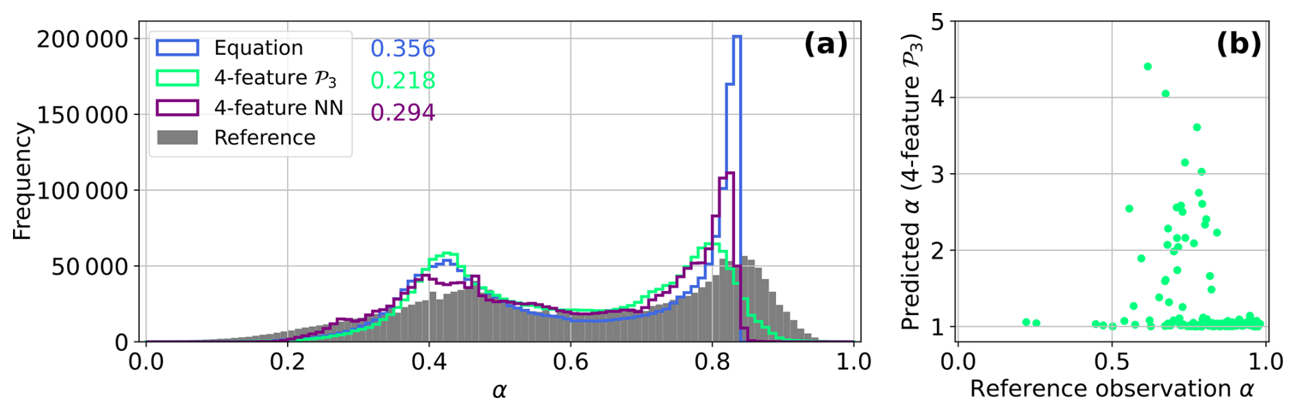
Figure 7 Comparison of the sea ice albedo distributions during the validation period (2019–2020) between the VIIRS product (Key et al., 2001, 2016) as reference observation and the predictions from the best-performing models in each model class in terms of MSE. Panel (a) illustrates the distribution of the reference observation alongside predictions from the best-performing equation (Eq. 4), the 4-feature polynomial of degree three 𝒫₃, and the 4-feature neural network (NN), all within the physical range between 0 and 1. The Hellinger distance for each model is shown next to the legend in their respective colors. Panel (b) shows predicted albedo values falling outside the physical range for the polynomial of degree three with four features, plotted against the observed sea ice albedo.

The three model predictions exhibit a bimodal distribution similar to the reference observation (with peaks at 0.46 and 0.84). Among the models, 4-feature 𝒫₃ shows the greatest similarity to the reference observation, with a Hellinger distance of 0.218 and MSE of 0.0145. This is followed by the 4-feature NN, with a Hellinger distance of 0.294 and MSE of 0.0133, and Eq. (4), with Hellinger distance of 0.356 and MSE of 0.0156. However, some of the predicted sea ice albedo values from 4-feature 𝒫₃ fall outside the physical range of 0 and 1, as illustrated in Fig. 7b, violating the first PC. Additionally, none of the models fully capture the long tail of the reference observation towards higher albedo values. Instead, both 4-feature NN and Eq. (4) demonstrate a notable peak at higher albedo values (0.82 and 0.83, respectively), with Eq. (4) having an upper limit for sea ice albedo at 0.83. The reference observation shows a peak of 0.84. Hence, the models exhibit a slight shift to the left. At the lower end of the albedo scale, the 4-feature NN best captures the long tail, although all model peaks at lower albedo values are more shifted to the left compared to the reference observation with a peak at 0.46: 0.42 for the 4-feature 𝒫₃, 0.39 for the 4-feature NN, and 0.42 for Eq. (4).

During training, we do not account for uncertainties associated with various satellite products. For the VIIRS product, the overall uncertainty for albedo retrieval is 0.1, and for surface temperature, it is 1.98 K, based on RMSE comparisons with in-situ measurements from the SHEBA campaign (Key et al., 2001, 2016). Light et al. (2022) assessed the albedo of eight individual sea ice surface types of sea ice based on field measurements from the MOSAiC expedition, finding that early autumn snow exhibits the highest albedo values between 0.8 and 0.9, while dark ponds have the lowest albedo values between 0.12 and 0.25. Thus, we conclude that the long tails of the albedo in the reference observation, values below 0.12 and above 0.9, are likely due to measurement, data processing, and retrieval errors. Moreover, our dataset has a spatial resolution of 25 km, which covers a variety of sea ice surface types, providing spatially averaged albedo values. In contrast, Light et al. (2022) reports highly localised albedo values for each surface type. Furthermore, as examined in Sect. 3.2.3, the lower and upper limits of Eq. (4) are determined by the coefficients $\stackrel{\mathrm{̃}}{a}=\mathrm{0.84}$ and $\stackrel{\mathrm{̃}}{b}=\mathrm{2.19}$, which have been optimised using the pan-Arctic dataset. With these coefficient values, Eq. (4) is unable to reproduce extreme albedo values. On the basis of these considerations, we infer that the upper albedo limits prescribed by Eq. (4) is physically plausible, given that the reference observation is noisy and reflects average albedo over a large area.

4.3 Spatial maps of sea ice albedo

Figure 8 illustrates the sea ice albedo exemplarily for 23 May 2020, with the reference observation (Fig. 8a), computed with the tuned PW79 (Fig. 8b), and Eq. (4) (Fig. 8c). Figure 8d and e depict deviations from the observed albedo. The tuned PW79 demonstrates two areas distinguishing between high and low albedo zones due to its constant albedo values representing surface types, namely snow-covered ice (α=0.66), and melting snow (α=0.40). As PW79 is not a smooth function, PW79 causes a sharp border between the two surface types. Conversely, the spatial variability of the observed albedo is better captured with Eq. (4), reducing the MSE by about a half (0.0156) compared to the tuned PW79 (0.0300). Biases remain in the Hudson Bay and along the sea ice edges, but are much reduced in the Central Arctic.

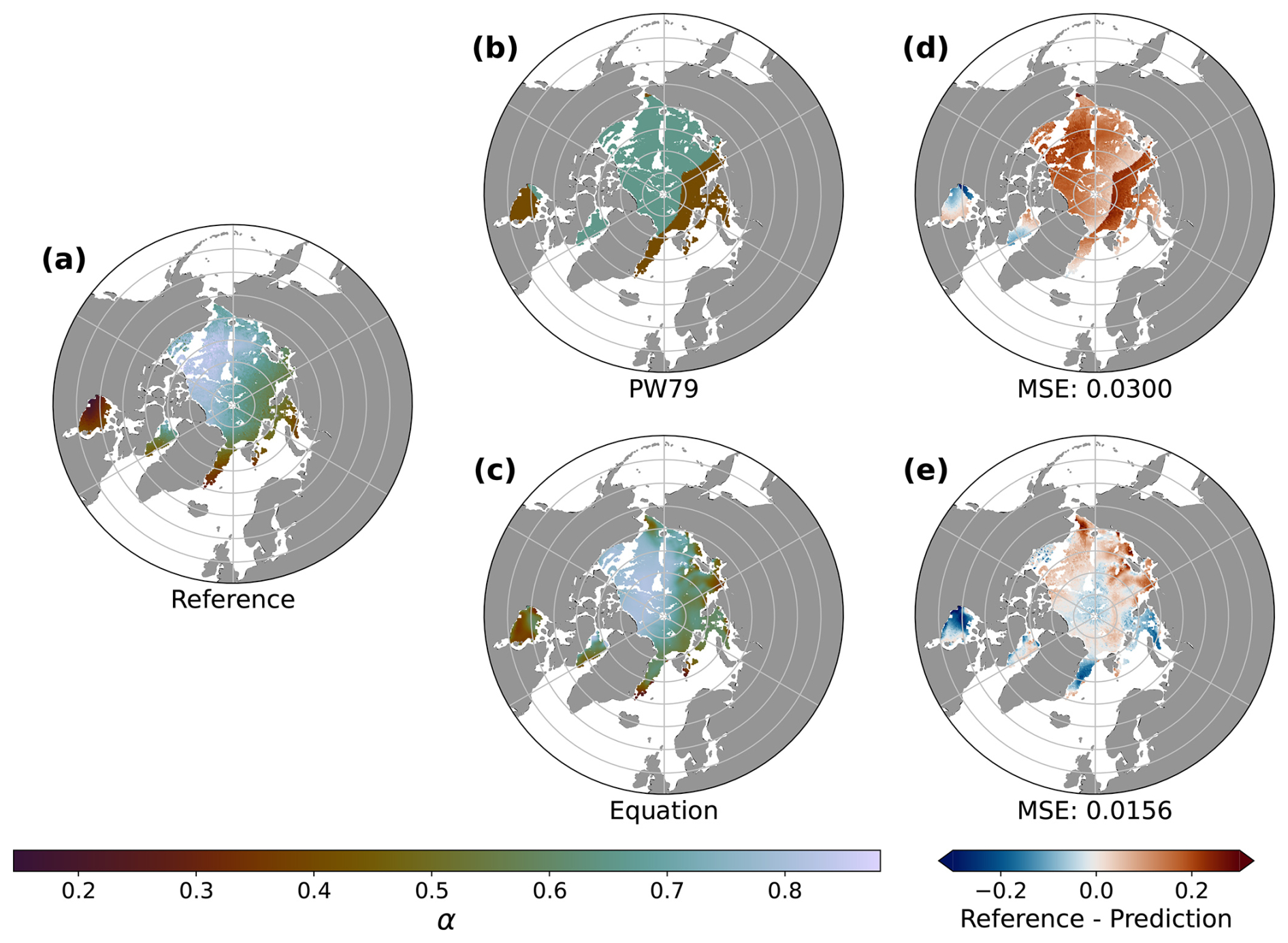
Figure 8 Comparison between (a) the sea ice albedo observed via the VIIRS satellite instrument (Key et al., 2001, 2016) as reference observation, (b) the tuned PW79, and (c) the best-performing equation (Eq. 4) for 23 May 2020. The deviations to the reference observation are illustrated in panel (d) for PW79 and panel (e) for Eq. (4).

4.4 Seasonal cycle of sea ice albedo

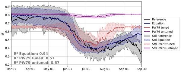
Figure 9 presents the seasonal albedo cycle of the reference observation, Eq. (4), and tuned and untuned PW79 for the period March–September. The data are averaged acrossed the years 2013–2020 to highlight the typical seasonal pattern and reduce interannual variability. For completeness, the seasonal cycles averaged seperately over the training period (2013–2018) and validation period (2019–2020) are provided in Appendix F, where they exhibit similar behaviour, indicating that the following analysis is robust across both training and validation periods.

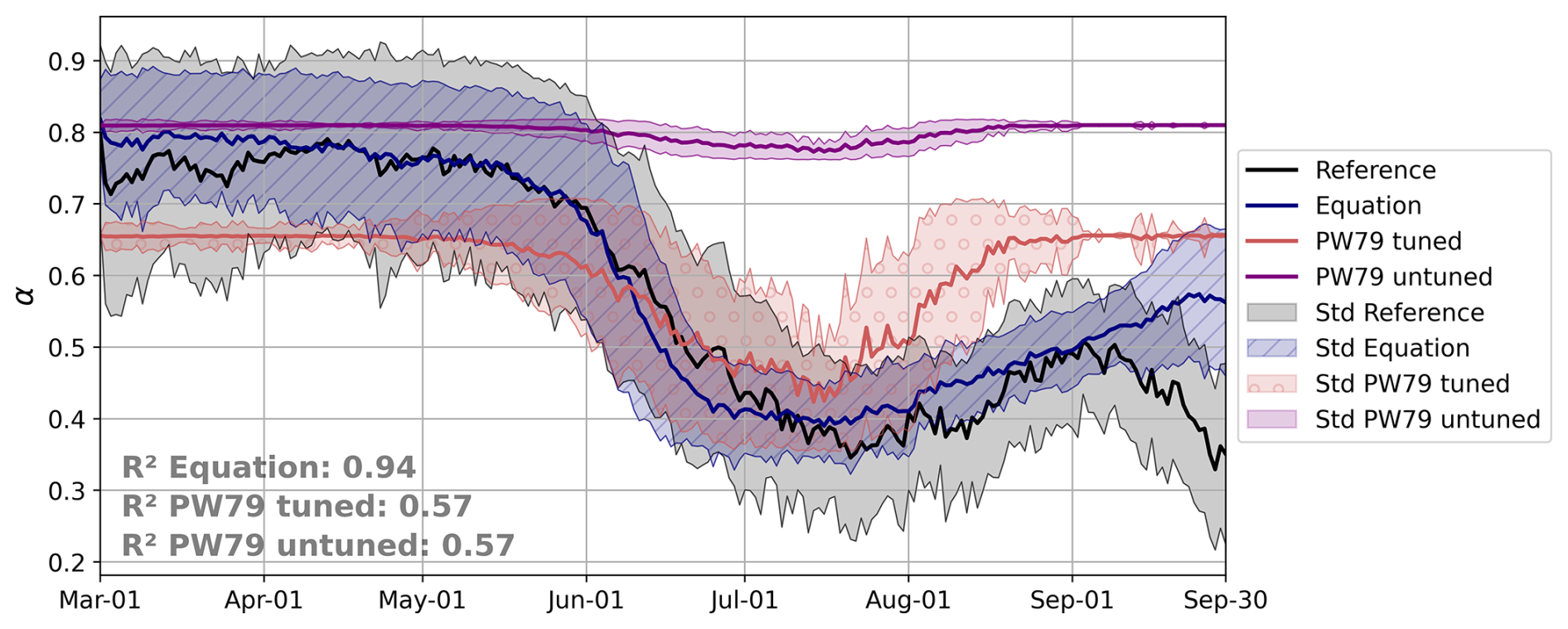
Figure 9 Seasonal sea ice albedo cycle from 1 March–30 September averaged from 2013 until 2020 observed via the VIIRS satellite instrument (Key et al., 2001, 2016) as reference observation, and computed with the best-performing equation (Eq. 4), and the sea ice albedo parametrisation by Parkinson and Washington (1979), here reffered to as PW79. The untuned PW79 corresponds to the standard configuration of the Finite-Element Sea Ice Model (FESIM; Danilov et al., 2015), while for a fair data-driven comparison, PW79 is tuned to the training set, including data from 2013–2018, using the Nelder–Mead method (Nelder and Mead, 1965).

The untuned PW79, unlike the other parametrisations, maintains a constant albedo at about 0.81, showing no seasonality. In contrast, the other three datasets display strong seasonality, with maximum sea ice albedo occurring during the winter period between March and April, followed by a steady decrease during the melting period between May and July, where it reaches its minimum. Equation (4) demonstrates a strong agreement with the reference observation, achieving an R² score of 0.94, whereas both untuned and tuned PW79 reach 0.57. During the winter period, the tuned PW79 starts with much lower albedo values around 0.66 compared to the reference observation and Eq. (4), which display sea ice albedo of similar magnitude of around 0.77. While the tuned PW79 reaches its minimum in July at 0.42, Eq. (4) reveals its minimum at 0.39, which is closer to the reference observation with 0.27. During the freeze-up period in August and September, the tuned PW79 demonstrates a rapid increase in sea ice albedo, similar in magnitude to the winter period. In contrast, the reference observation and Eq. (4) depict a more gradual increase, with sea ice albedo not recovering as rapidly to winter magnitude in August.

While Eq. (4) remains gradually increasing in September, the reference observation shows a decrease of sea ice albedo, which contradicts the expected freeze-up behaviour of Arctic sea ice (Pistone et al., 2014; Light et al., 2022). Peng et al. (2018) showed that the quality and accuracy of the VIIRS albedo product decrease with increasing solar zenith angle in September. Despite being trained on the reference observation, Eq. (4) provides a more physically reasonable prediction for September, likely due to the sparse observational data available for that month, as reduced sunlight over the pole limits September data availability (see Appendix E), resulting in less weight being given to these observations during training. Therefore, PySR relies more heavily on the complete data from March–August (see Fig. 2). As a result, PySR implicitly captures seasonal patterns, particularly temperature-driven trends (see Sect. 3.2.2), which extend naturally into September. In doing so, Eq. (4) effectively corrects for potential measurement artefacts in the September data by leveraging the functional relationships between ΔT^* and α learnt from better sampled months.

Both tuned and untuned PW79 exhibit very low standard deviations during the winter period and September, with higher values around 0.13 during the melting season for the tuned PW79. Conversely, the reference observation shows high standard deviations with a maximum of 0.19, which are attributed to the spatial variability of sea ice albedo and measurement, data processing, and retrieval errors as already discussed in Sect. 4.2. Equation (4) reveals lower standard deviations with a maximum of 0.16, potentially eliminating errors, and are attributed solely to the spatial variability of the albedo. The low standard deviations in the tuned and untuned PW79 stem from its simplistic nature, relying on constant albedo values based on snow cover and surface temperature, where each constant represents a sea ice surface type. This results in PW79 perceiving the sea ice as highly uniform during the winter and September, whereas the tuned PW79 captures more variability during the melting season.

Overall, Eq. (4) presents a clear improvement over PW79, aligning with observed sea ice albedo variations by capturing both the seasonal progression and its magnitude. The untuned PW79 does not capture the observed albedo seasonality, maintaining a high value of 0.81 year-round. It should be noted that the sea ice albedo is calculated for each of these methods with observed melting conditions, which could differ from the conditions in FESIM.

Although the tuned PW79 better captures sea ice albedo seasonality, it significantly deviates in magnitude, inaccurately reflecting albedo changes and showing an earlier, quicker freeze-up than the reference observation. Both the reference observation and Eq. (4) align with previous field campaigns from SHEBA (Perovich et al., 2002) and MOSAiC (Light et al., 2022), identifying five phases of Arctic sea ice: dry snow (March–Aril), melting snow (May), pond formation (June), pond development (July), and freeze-up (August–September). It is noticeable that these studies were based on highly localised measurements, whereas this study investigates spatially averaged data over a 25 km resolution.

5 Regional and monthly optimisation of Eq. (4)

5.1 Comparison between the optimisation strategies

Figure 8e reveals regional differences in model performance for Eq. (4), suggesting that the global optimisation approach on the entire training set is not able to capture the underlying patterns uniformly across all regions. This finding motivates us to explore spatial and temporal variations in model performance by conducting optimisations on regional and monthly subsets. As Eq. (4) provides physically meaningful coefficients, as demonstrated in Sect. 3.2.3, we are able to gain insights into the underlying physical mechanisms governing model performance. In contrast, optimising NNs on subsets would not offer the same level of interpretability due to their inherent black-box nature. To ensure consistency across all subset optimisations, we divide our training set into monthly and regional subsets, utilising 20 000 data samples for each region and 10⁵ data points for each month.

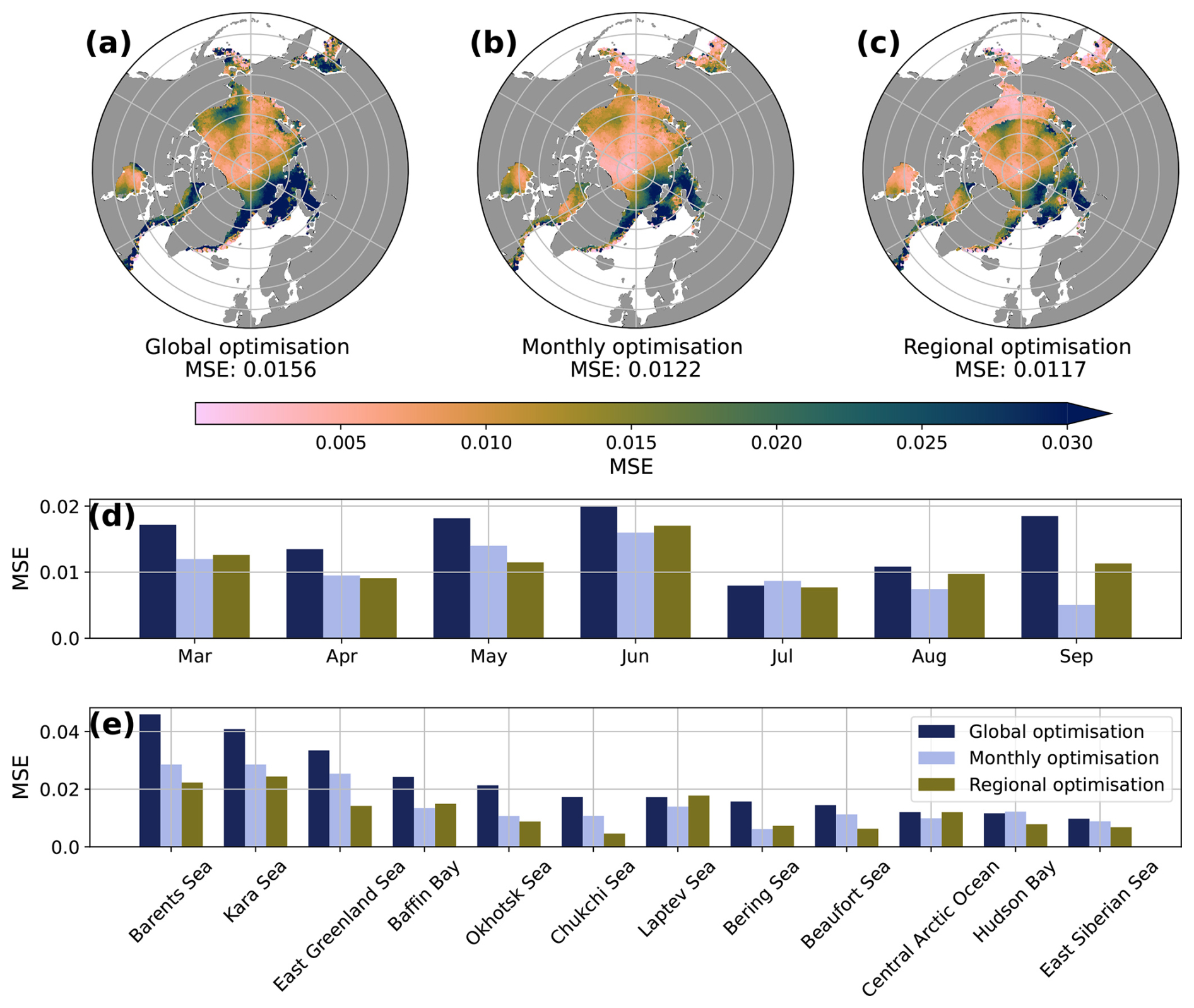
Figure 10 Monthly and regional analysis. Panels (a)–(c) illustrate the mean squared error on the validation set (MSE) for each grid cell for the global, monthly, and regional optimisation, respectively. Panels (d) and (e) show the MSE for each month and region, respectively, when fine-tuning Eq. (4) globally (brown), on each month (green), and on each region (red).

Both monthly (MSE=0.0122) and regional (MSE=0.0117) optimisation strategies outperform global optimisation (MSE=0.0156) in terms of reducing overall MSE (Fig. 10a–c) albeit making the coefficients depend on the region or month greatly increases the complexity of Eq. (4). This improvement is likely due to the ability of Eq. (4) to capture regional and monthly variations in the data. The regional optimisation approach leads to significant reductions in MSE for certain regions, such as the Barents Sea (from 0.0460–0.0220), Kara Sea (from 0.0409–0.0263), and East Greenland Sea (from 0.0335–0.0148) (Fig. 10e). However, these regions, which border the North Atlantic, continue to exhibit high MSEs across all optimisation strategies, suggesting that they may be influenced by physical processes not well-represented by Eq. (4), such as Atlantic Oceanic heat transport or strong winds prevailing in these regions (Screen and Simmonds, 2010; Årthun et al., 2012; Liu et al., 2024). Another potential reason is that the underlying physics operate on a time scale smaller than our data, which are on a daily basis due to the temporal resolution of the satellite data.

In terms of the magnitude of improvement, regional optimisation yields higher proportional improvements compared to monthly optimisation (Fig. 10d and e). The greatest proportional improvements in the reduction of MSE are observed for the Chuckshi Sea with regional optimisation (75 %), September with monthly optimisation (69 %), and the Beaufort Sea (59 %). However, the Central Arctic shows little improvement with regional optimisation, likely due to its dominant representation in the dataset (64 % of the entire dataset). As a result, the global optimisation is already greatly influenced by the Central Arctic data, and the optimal coefficients are likely biased towards this region, leaving little room for improvement with regional optimisation.

One limitation of the regional optimisation approach is that it produces sharp borders in the error map (Fig. 10c), reflecting the regional focus of the optimisation process, which leads to a lack of a smooth error transitions between regions. Additionally, some instances of overfitting are observed, where regional or monthly optimisation results in high MSE values compared to global optimisation. For example, the MSE of July with monthly optimisation (0.0088) is higher than with global optimisation (0.0080), and similar patterns are seen for Hudson Bay with regional optimisation (0.0138 vs. 0.00116), and Laptev Sea with regional optimisation (0.0185 vs. 0.0172).

5.2 Case study: Barents Sea

The optimised coefficients for each region and month resulting in the analysis in Sect. 5.1 are displayed in Appendix G and Appendix H, respectively. Physical interpretation of each region and month goes beyond the scope of this study. Instead, we focus on the Barents Sea as a case study. This region exhibits the highest MSE from global optimisation and significant improvement with regional optimisation. For a direct comparison, the coefficients are standardised to their unitless form (Table 3).

Table 3 Unitless coefficients, divided by the respective standard deviations of the training set (2013–2018), for the whole dataset representing the entire pan-Arctic region and Barents Sea, optimised on the validation period (2019–2020).

In the Barents Sea, the effect of h_snow becomes significantly smaller (${\stackrel{\mathrm{̃}}{p}}_{\text{snow, std}}=\mathrm{0.03}$) compared to the pan-Arctic region (${\stackrel{\mathrm{̃}}{p}}_{\text{snow}}=\mathrm{0.85}$), while h_ice becomes more important (${\stackrel{\mathrm{̃}}{p}}_{\text{ice,std}}=\mathrm{0.64}$) than in the pan-Arctic region (${\stackrel{\mathrm{̃}}{p}}_{\text{ice,std}}=\mathrm{0.09}$). These differences reflect the distinct physical conditions in these regions. The Barents Sea experiences high seasonality, with thin sea ice prevalent and little to no snow present, compared to the whole pan-Arctic region (Smedsrud et al., 2013). Consequently, variations in thin sea ice play a more significant role in α in the Barents Sea, whereas variations in thin snow influence α in the pan-Arctic region.

In both cases, T_0 m has the highest weight (of around 2). However, T_2 m is less significant in the Barents Sea (${\stackrel{\mathrm{̃}}{p}}_{T_{\mathrm{2}\mathrm{m}},\text{std}}=\mathrm{0.34}$) than in the pan-Arctic region (${\stackrel{\mathrm{̃}}{p}}_{T_{\mathrm{2}\mathrm{m}},\text{std}}=\mathrm{0.99}$). In the pan-Arctic region ($\stackrel{\mathrm{̃}}{c}=\mathrm{0.95}$), smaller ΔT^* are required to trigger melting, while in the Barents Sea, the lower value of $\stackrel{\mathrm{̃}}{c}=-\mathrm{0.04}$ triggers melting conditions already at higher ΔT^*. The shift of the transition to higher ΔT^* implies other heat sources affecting sea ice optical properties which are not considered in Eq. (4), as already discussed in 5.1.

Our findings indicate that the pan-Arctic region represents a stable ice regime, in which snow and small ΔT^* modulate α, while the Barents Sea represents a fragile ice regime, where ice properties and temperatures already at higher ΔT^* regulate α sensitivity. The Barents Sea is one of the most rapidly changing regions, becoming ice-free in summer and contributing to approximately one-quarter of the Arctic sea ice loss in winter. This change is associated with surface warming in the Gulf Stream and the increase of the Atlantic oceanic heat transport passing the Barents Sea Opening (Yamagami et al., 2022; Årthun et al., 2012; Smedsrud et al., 2013; Stroeve and Notz, 2018).

This case study gives a first insight on how Eq. (4) can be transferred to different ice regimes, specifically from a stable, pan-Arctic regime dominated by multiyear ice in the Central Arctic to a fragile ice regime characteristic of the Barents Sea. Although we acknowledge that the MSE in the Barents Sea remains relatively high compared to other regions after fine-tuning (see Sect. 5.1), the functional form of Eq. (4) remains physically reasonable. This enables a comparison between the coefficients obtained from global and regional optimisations demonstrating that the optimal coefficients are state-dependent.

6 Conclusions

In this study, we derived an interpretable, physically consistent equation for sea ice albedo through the integration of several multi-year satellite and reanalyses data covering the pan-Arctic region and the application of various machine learning techniques, including NNs, SFS, and symbolic regression with PySR. Our best-performing data-driven equation (Eq. 4) combines two mechanisms that critically impact sea ice albedo, likely optimised for the Central Arctic since this region dominates our dataset (64 %): high sensitivity to small changes in thin snow, and the temperature difference between the sea ice surface and 2 m air, weighted in a way such as to reflect the current season. While the PW79 sea ice albedo parametrisation only uses the surface temperature as a proxy to define freezing and melting conditions, our equation shows that a weighted temperature difference between the surface and the air at 2 m better encodes information on the seasonal cycle. As our physical interpretation could be influenced by the warm 2 m air temperature biases in ERA5, other possible predictors that encode information on the seasonal cylce, such as solar insolation or the surface energy balance, could be explored in future work.

The error-complexity graph demonstrates that NNs are overly complex and that lower-complexity models are sufficient to achieve comparable performance. Equation (4) significantly outperforms PW79, reducing the MSE on the observational validation set by half and improving the representation of the spatial variability and seasonal cycle of sea ice albedo. Moreover, Eq. (4) sets lower and upper limits for sea ice albedo due to the functional behaviour of the hyperbolic tangent that are physically plausible and yield realistic sea ice albedo values. By adapting the coefficients of Eq. (4) to subsets of the dataset, it demonstrates its flexibility in regional and monthly assessments, allowing for a more in-depth analysis of the underlying physics within each subset as the optimised coefficients can be directly interpreted.

One methodological constraint in our approach is the selection of features that are available on a daily basis across the entire pan-Arctic region and are also represented in sea ice models with implicit melt pond treatment. This deliberate feature selection ensures compatibility with our modelling objectives, but overlooks other relevant factors that may substantially impact sea ice albedo. For example, snow grain size (Perovich, 1996; Perovich et al., 2002) or black carbon (Hansen and Nazarenko, 2004) substantially determine sea ice/snow albedo, but there is no data available on a daily, pan-Arctic scale. Furthermore, melt ponds are known to significantly reduce sea ice albedo, as demonstrated in numerous studies (e.g. Perovich et al., 2002; Webster et al., 2022; Niehaus et al., 2025). Yet, accurately representing melt ponds in ESMs remains challenging since melt pond evolution is highly sensitive to environmental conditions and small-scale processes such as ice topography and drainage (Popović et al., 2020; Smith et al., 2025). These processes cannot be explicitly resolved and must be parametrised, potentially introducing biases (Smith et al., 2025). Equation (4) provides a promising alternative for sea ice models that employ an implicit melt pond treatment, while explicit melt pond schemes remain pivotal for robust polar climate projections. Since the objective of this study is to capture large-scale patterns at 25×25 km² resolution, Eq. (4) sufficiently explains the variance in observed sea ice albedo, indicating that small-scale features may have a limited marginal effect at this scale.

Another consideration of our approach is that this study aimed to minimise global MSE on the validation set, with the Central Arctic dominating the dataset spatially and temporally. As this mirrors present-day conditions, other subregions are underrepresented in our dataset where the impact of climate change is more pronounced such as the Barents Sea. Consequently, the ranking resulting from SFS and Eq. (4) is likely optimised for the Central Arctic, as evident from monthly and regional differences in MSE. To balance the data, dominant subregions or months could be downsampled, which results in a more diverse training set, but this would most likely lead to a higher MSE overall.

To test Eq. (4) offline on new datasets such as regional subsets or other observational or reanalysis products, we recommend following our fine-tuning workflow as we did exemplarily in Sect. 5: split the data into training and validation periods, standardise the data, fine-tune the coefficients on the training set, and evaluate the validation MSE. If Eq. (4) does not perform well, this indicates that the underlying functional behaviour of the new dataset differs. In this case, we recommend repeating the entire workflow and identifying alternative symbolic forms that better describe the data.

An important question concerns how well Eq. (4) generalises well beyond Arctic sea ice regimes represented in the training data. Ship-based field measurements in the Antarctic by Brandt et al. (2005) and Tersigni et al. (2025) demonstrate that already a thin snow layer of a few centimetres substantially increases sea ice albedo, emphasising that snow fractional coverage is more impactful than snow thickness. Here, snow redistribution is mainly driven by strong winds, particularly in the marginal ice zones. Since our dataset has a spatial resolution of 25 km, retrieved h_snow likely reflects a combination of snow thickness and fractional coverage. The strong sensitivity of Eq. (4) to small variations in thin snow therefore suggests that the influence of snow on albedo is captured in a physically meaningful way. Nevertheless, Sect. 5 indicates that the optimal coefficients of Eq. (4) are state-dependent. While the functional form remains transferable, as demonstrated by the Barents Sea case study, the relatively high MSE in this region after fine-tuning suggests that additional processes, such as oceanic heat fluxes, may drive sea ice albedo but are not explicitly represented in Eq. (4). Oceanic heat fluxes also drive sea ice melt in the Antarctic (Brandt et al., 2005), which may influence sea ice albedo, implying that further offline investigations are required to assess the robustness of the parametrisation outside the pan-Arctic region. This is presently limited due to the lack of data availability on a daily, Antarctic scale.

In practice, Eq. (4) naturally retains a degree of tunability that facilitates its online implementation in a global model. Integrating Eq. (4) into an ESM or operational sea ice forecast model would not require substantial changes in existing tuning protocols, as the parameter space can simply be expanded by the seven coefficients of Eq. (4) to obtain physically plausible sea ice states. Under different atmospheric forcings, either in an ocean–sea-ice stand-alone configuration driven by an atmospheric reanalysis product or in a fully coupled configuration, we hypothesise that distinct optimal values of these coefficients will emerge, particularly those controlling ΔT^* where the sea ice model receives T_2 m from the atmosphere, since biases in atmospheric temperature fields vary across forcing datasets (Batrak and Müller, 2019). This highlights the potential value of regime-aware parametrisations, as suggested by Nath et al. (2026), in which the parameter space is dynamically adjusted in response to the prevailing climate state, allowing the scheme to remain applicable across Arctic, Antarctic, and potentially future or paleoclimate sea ice regimes.

Overall, our results suggest that the functional form of Eq. (4) provides a physically interpretable representation of sea ice albedo variability, while the globally optimised coefficient set may not remain optimal across different regions or climate states. Yet, the explicit formulation and limited number of coefficients make the parametrisation well suited for online implementation in ESMs or sea ice forecasts, where the coefficients can be tuned to the model’s specific climate regime. Further evaluation, particularly in Antarctic conditions and under future or paleoclimate conditions, will be necessary to assess the broader applicability of the approach.

This study demonstrates the first use of interpretable ML in sea ice modelling to foster trust and transparency in the Earth system community. Bridging a gap between the ML and the Earth system science community, we leveraged interpretable ML techniques to gain a deeper understanding of the physical mechanisms driving sea ice albedo. Our approach contributes to the growing body of research that establishes ML as a valuable tool in Earth system science, with applications in data assimilation, numerical weather predictions, and climate emulators.

Appendix A: Correlation matrices

A1 Comparison between observational and reanalysis data for March and April (2013–2020)

Satellite instruments are not able to reliably retrieve h_snow and h_ice during the summer months (May-September) due to the presence of melt ponds which distort the signal coming from the snow and sea ice (Rostosky et al., 2018; Ricker et al., 2017). To fill the data gaps, reanalysis data seem to be useful as they provide spatio-temporal coverage assimilated with observational data. To assess whether filling data gaps with reanalysis data is appropriate, Fig. A1 compares the correlation matrices of the datasets for the period March until mid April from 2013–2020 with h_snow and h_ice retrieved from satellite observations (Table 1 and Fig. A1a), and from the Arctic Ocean Physics Reanalysis TOPAZ4b (Fig. A1b). The correlation matrices of both datasets look similar as the linear correlations between all features have the same signs of comparable magnitude, which justifies using TOPAZ4b for h_snow and h_ice to fill the gaps during the summer months.

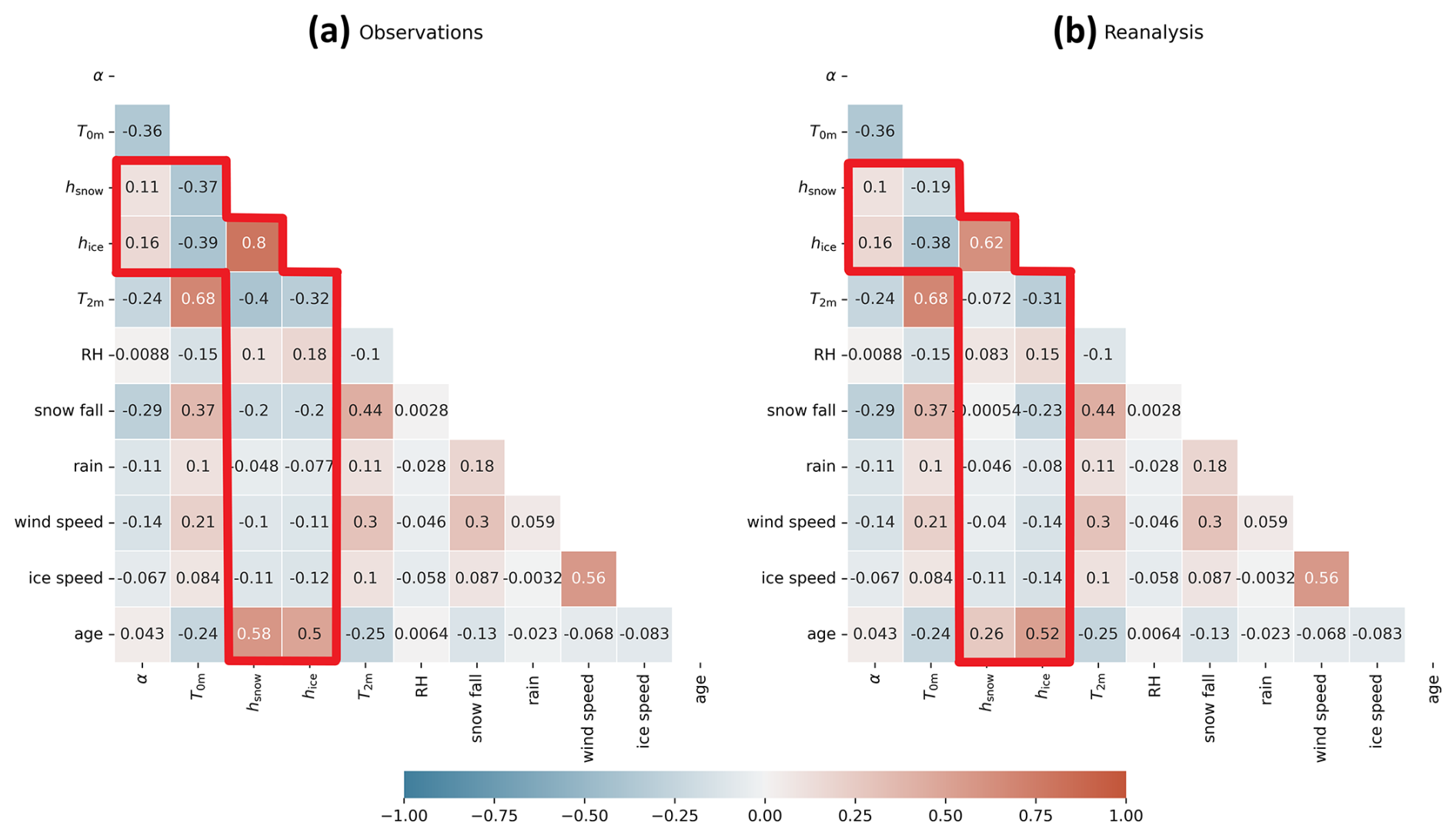
Figure A1 Correlation matrices for comparing snow (h_snow) and sea ice thickness (h_ice) data retrieved from (a) the satellite observations AMSR2 (Rostosky et al., 2018) and CS2SMOS (Ricker et al., 2017), respectively, and (b) Arctic Ocean Physics Reanalysis TOPAZ4b (European Union-Copernicus Marine Service, 2020) from March until mid April (2013–2020). The red marking indicates the comparing linear correlations between satellite observations and reanalysis.

A2 Correlation matrix of final dataset (from March until September 2013–2020)

Figure A2 presents the correlation matrix of the preprocessed dataset from several data products as described in Table 1, consisting of data from March until September from 2013–2020.

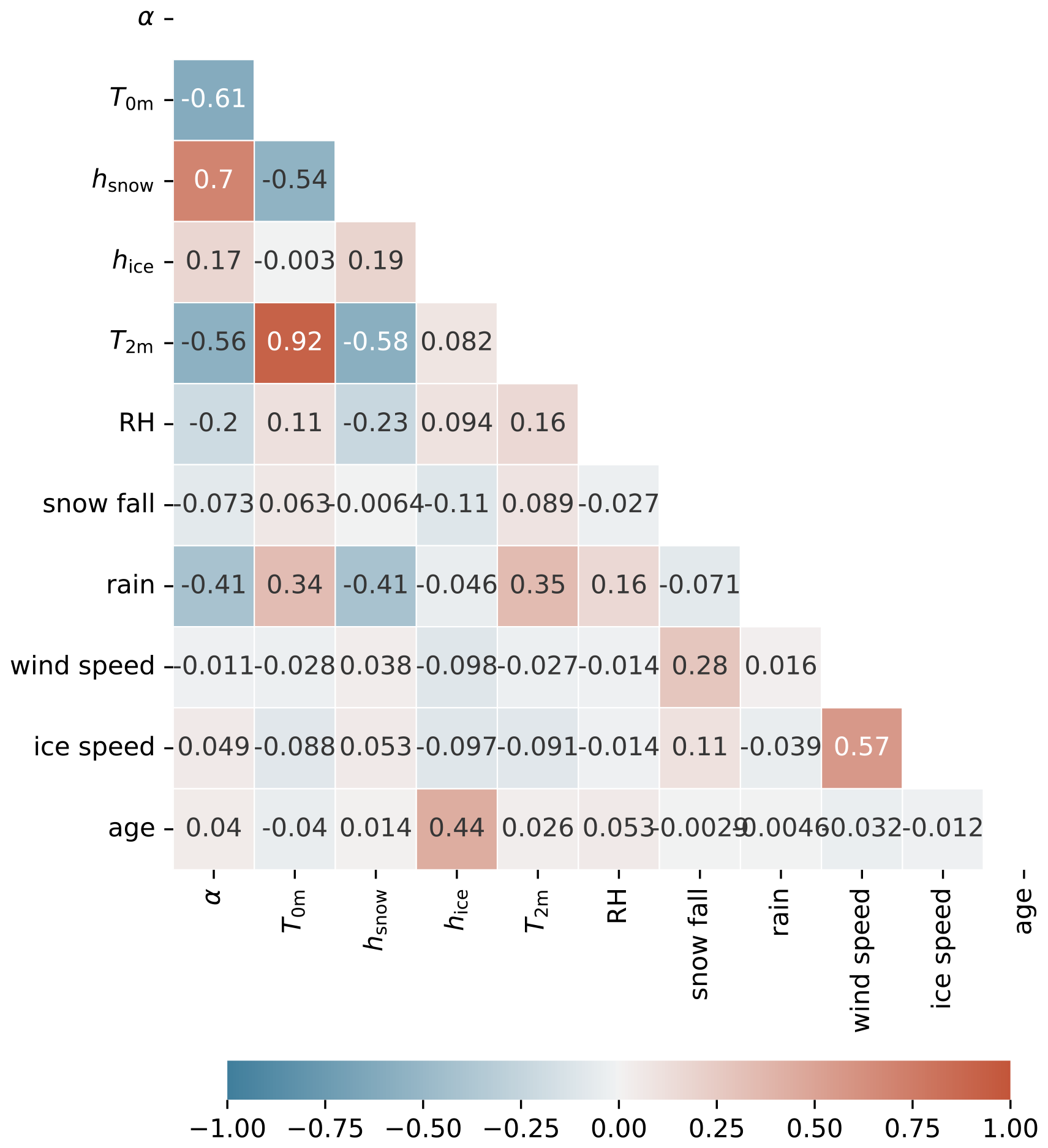
Figure A2 Correlation matrix of preprocessed dataset from several data products (Table 1. From March until mid April, h_snow and h_ice are retrieved from satellite observations (Rostosky et al., 2018; Ricker et al., 2017). The data gaps from mid April until September are filled with the Arctic Ocean Physics Reanalysis TOPAZ4b (European Union-Copernicus Marine Service, 2020) as described in Sect. 2.1.2.

Appendix B: Mean values of the features during the validation period (2019–2020)

Table B1 shows the mean values of the features h_snow, h_ice, T_0 m and T_2 m during the validation period (2019–2020).

Table B1 Mean values of the features during the validation period (2019–2020).

Appendix C: Selected Symbolic Regression Fits

The best-performing equations discovered by PySR are listed that satisfy the PCs (see Sect. 2.2.4) and showcased in Fig. 6, ranked in increasing MSE order with the MSE/number of parameters in brackets. Equations (C1)–(C3) are optimised with the Nelder–Mead solver, and Eqs. (C4) and (C5) with the BFGS-solver. Note that the equations are shown in their standardised form following Eq. (1). Equations (C1), (C3) and (C5) are Pareto-optimal, which are denoted in bold:

1. [0.155/7]:

   $$\begin{array}{}\text{(C1)}& \begin{array}{rl}{\displaystyle }& {\displaystyle }\mathit{\alpha }(h_{\text{ice}},h_{\text{snow}},T_{\mathrm{2}\mathrm{m}},T_{\mathrm{0}\mathrm{m}})=\\ {\displaystyle }& {\displaystyle }{\displaystyle \frac{{\tanh }^{\mathrm{2}}(\mathrm{0.09}{h}_{\text{ice}}+\mathrm{0.85}{h}_{\text{snow}}^{\mathrm{2}}+\mathrm{0.84})}{\mathrm{2.19}-\tanh (\mathrm{0.98}{T}_{\mathrm{2}\mathrm{m}}-\mathrm{2.17}{T}_{\mathrm{0}\mathrm{m}}+\mathrm{0.93})}}\end{array}\end{array}$$

2. [0.0159/8]:

   $$\begin{array}{}\text{(C2)}& \begin{array}{rl}{\displaystyle }& {\displaystyle }\mathit{\alpha }(h_{\text{ice}},h_{\text{snow}},T_{\mathrm{0}\mathrm{m}})=\\ {\displaystyle }& {\displaystyle }{\left(-\mathrm{0.92}+{\displaystyle \frac{\sqrt{\mathrm{0.32}+(\mathrm{0.83}{T}_{\mathrm{0}\mathrm{m}}+\mathrm{0.35}{)}^{\mathrm{2}}}}{\begin{array}{l}\mathrm{1.05}{h}_{\text{ice}}\sqrt{h_{\text{snow}}}\\ +\mathrm{1.52}{\left(\mathrm{1.04}{h}_{\text{snow}}^{\mathrm{2}}{T}_{\mathrm{0}\mathrm{m}}^{\mathrm{2}}+\mathrm{1.18}\right)}^{\mathrm{2}}\end{array}}}\right)}^{\mathrm{2}}\end{array}\end{array}$$

3. [0.0161/6]:

   $$\begin{array}{}\text{(C3)}& \begin{array}{rl}{\displaystyle }& {\displaystyle }\mathit{\alpha }(h_{\text{ice}},h_{\text{snow}},T_{\mathrm{0}\mathrm{m}})=\mathrm{0.83}\\ {\displaystyle }& {\displaystyle }\times {\left(\mathrm{1}+{\displaystyle \frac{-\mathrm{0.43}}{\begin{array}{l}\mathrm{1.74}{h}_{\text{snow}}^{\mathrm{4}}{T}_{\mathrm{0}\mathrm{m}}^{\mathrm{4}}\\ +\sqrt{\mathrm{2.01}{h}_{\text{ice}}^{\mathrm{2}}{h}_{\text{snow}}+|-\mathrm{0.95}{T}_{\mathrm{0}\mathrm{m}}+\mathrm{1.70}|}\end{array}}}\right)}^{\mathrm{2}}\end{array}\end{array}$$

4. [0.0162/7]:

   $$\begin{array}{}\text{(C4)}& \begin{array}{rl}{\displaystyle }& {\displaystyle }\mathit{\alpha }(h_{\text{ice}},h_{\text{snow}},T_{\mathrm{0}\mathrm{m}})=\mathrm{0.84}\\ {\displaystyle }& {\displaystyle }\times {\left(\mathrm{1}+{\displaystyle \frac{-\mathrm{0.66}}{\begin{array}{l}\mathrm{0.83}{h}_{\text{ice}}\sqrt{h_{\text{snow}}}+{\left(\mathrm{1.18}{h}_{\text{snow}}^{\mathrm{2}}{T}_{\mathrm{0}\mathrm{m}}-\mathrm{1}\right)}^{\mathrm{2}}\\ +{\left(-\mathrm{0.71}{T}_{\mathrm{0}\mathrm{m}}^{\mathrm{2}}-\mathrm{0.68}{T}_{\mathrm{0}\mathrm{m}}+\mathrm{0.97}\right)}^{\mathrm{2}}\end{array}}}\right)}^{\mathrm{2}}\end{array}\end{array}$$

5. [0.0180/5]:

   $$\begin{array}{}\text{(C5)}& \begin{array}{rl}{\displaystyle }& {\displaystyle }\mathit{\alpha }(h_{\text{snow}},T_{\mathrm{0}\mathrm{m}})=\\ {\displaystyle }& {\displaystyle }\mathrm{0.84}{\left(\mathrm{1}+{\displaystyle \frac{-\mathrm{0.79}}{\mathrm{2.04}\sqrt{h_{\text{snow}}}+(\mathrm{1.24}{h}_{\text{snow}}^{\mathrm{2}}{T}_{\mathrm{0}\mathrm{m}}-\mathrm{1.55}{)}^{\mathrm{2}}}}\right)}^{\mathrm{2}}\end{array}\end{array}$$

Equations (C1)–(C5) are retrieved using different PySR configurations, which are shown in Table C1. Note that here, Eq. (C1) equals Eq. (4) in the main text. The hypothesis space refers to the symbolic operators that PySR has access to within a run.

Exploring the dependency of α on h_snow and h_ice in Fig. C1, all PySR equations without a hyperbolic tangent function approximate a saturating behaviour, therefore the physical interpretation demonstrated in Sect. 3.2.1 also holds for the other PySR equations.

Table C1 Configurations of PySR runs.

Figure C1 Comparison of the responses of the candidate equations to varying snow depth (h_snow) and sea ice thickness (h_ice), complementary to Fig. 3. Equation (C1) equals Eq. (4) in the main text.

Appendix D: 4-feature polynomial of degree three 𝒫₃

Equation (D1) represents the 4-feature polynomial of degree three 𝒫₃ for which the distribution of predicted sea ice albedo during the validation period (2019–2020) is shown in Fig. 7. 𝒫₃ consists of the features $h_{\text{snow}},T_{\mathrm{0}\mathrm{m}},T_{\mathrm{2}\mathrm{m}},h_{\text{ice}}$. Note that Eq. (D1) is shown in its standardised form following 1.

$$\begin{array}{}\text{(D1)}& \begin{array}{rl}{\displaystyle }& {\displaystyle }\mathit{\alpha }(h_{\text{snow}},T_{\mathrm{0}\mathrm{m}},T_{\mathrm{2}\mathrm{m}},h_{\text{ice}})=\\ {\displaystyle }& {\displaystyle }\mathrm{0.2266}+\mathrm{0.3046}{h}_{\text{snow}}-\mathrm{0.1694}{T}_{\mathrm{0}\mathrm{m}}+\mathrm{0.0129}{T}_{\mathrm{2}\mathrm{m}}\\ {\displaystyle }& {\displaystyle }+\mathrm{0.1331}{h}_{\text{ice}}-\mathrm{0.1385}{h}_{\text{snow}}^{\mathrm{2}}-\mathrm{0.1267}{h}_{\text{snow}}{T}_{\mathrm{0}\mathrm{m}}\\ {\displaystyle }& {\displaystyle }-\mathrm{0.0212}{h}_{\text{snow}}{T}_{\mathrm{2}\mathrm{m}}+\mathrm{0.0159}{h}_{\text{snow}}{h}_{\text{ice}}-\mathrm{0.0928}{T}_{\mathrm{0}\mathrm{m}}^{\mathrm{2}}\\ {\displaystyle }& {\displaystyle }+\mathrm{0.0081}{T}_{\mathrm{0}\mathrm{m}}{T}_{\mathrm{2}\mathrm{m}}+\mathrm{0.0116}{T}_{\mathrm{0}\mathrm{m}}{h}_{\text{ice}}+\mathrm{0.0254}{T}_{\mathrm{2}\mathrm{m}}^{\mathrm{2}}\\ {\displaystyle }& {\displaystyle }+\mathrm{0.0687}{T}_{\mathrm{2}\mathrm{m}}{h}_{\text{ice}}-\mathrm{0.0313}{h}_{\text{ice}}^{\mathrm{2}}+\mathrm{0.0087}{h}_{\text{snow}}^{\mathrm{3}}\\ {\displaystyle }& {\displaystyle }+\mathrm{0.0055}{h}_{\text{snow}}^{\mathrm{2}}{T}_{\mathrm{0}\mathrm{m}}-\mathrm{0.0062}{h}_{\text{snow}}^{\mathrm{2}}{T}_{\mathrm{2}\mathrm{m}}\\ {\displaystyle }& {\displaystyle }+\mathrm{0.0097}{h}_{\text{snow}}^{\mathrm{2}}{h}_{\text{ice}}-\mathrm{0.0180}{h}_{\text{snow}}{T}_{\mathrm{0}\mathrm{m}}^{\mathrm{2}}\\ {\displaystyle }& {\displaystyle }+\mathrm{0.0287}{h}_{\text{snow}}{T}_{\mathrm{0}\mathrm{m}}{T}_{\mathrm{2}\mathrm{m}}+\mathrm{0.0210}{h}_{\text{snow}}{T}_{\mathrm{0}\mathrm{m}}{h}_{\text{ice}}\\ {\displaystyle }& {\displaystyle }-\mathrm{0.0469}{h}_{\text{snow}}{T}_{\mathrm{2}\mathrm{m}}^{\mathrm{2}}-\mathrm{0.0132}{h}_{\text{snow}}{T}_{\mathrm{2}\mathrm{m}}{h}_{\text{ice}}\\ {\displaystyle }& {\displaystyle }-\mathrm{0.0050}{h}_{\text{snow}}{h}_{\text{ice}}^{\mathrm{2}}-\mathrm{0.0193}{T}_{\mathrm{0}\mathrm{m}}^{\mathrm{3}}+\mathrm{0.0125}{T}_{\mathrm{0}\mathrm{m}}^{\mathrm{2}}{T}_{\mathrm{2}\mathrm{m}}\\ {\displaystyle }& {\displaystyle }-\mathrm{0.0144}{T}_{\mathrm{0}\mathrm{m}}^{\mathrm{2}}{h}_{\text{ice}}-\mathrm{0.0047}{T}_{\mathrm{0}\mathrm{m}}{T}_{\mathrm{2}\mathrm{m}}^{\mathrm{2}}\\ {\displaystyle }& {\displaystyle }+\mathrm{0.0218}{T}_{\mathrm{0}\mathrm{m}}{T}_{\mathrm{2}\mathrm{m}}{h}_{\text{ice}}-\mathrm{0.0093}{T}_{\mathrm{0}\mathrm{m}}{h}_{\text{ice}}^{\mathrm{2}}+\mathrm{0.0011}{T}_{\mathrm{2}\mathrm{m}}^{\mathrm{3}}\\ {\displaystyle }& {\displaystyle }+\mathrm{0.0070}{T}_{\mathrm{2}\mathrm{m}}^{\mathrm{2}}{h}_{\text{ice}}+\mathrm{0.0028}{T}_{\mathrm{0}\mathrm{m}}{h}_{\text{ice}}^{\mathrm{2}}+\mathrm{0.0026}{h}_{\text{ice}}^{\mathrm{3}}\end{array}\end{array}$$

Appendix E: Comparison of spatial maps between the VIIRS product and Eq. (4)

Figure E1 shows the differences in spatial maps between the VIIRS product (reference observation) and Eq. (4) exemplarily for 1, 15 and 30 September 2018.

Figure E1 Comparison of sea ice albedo maps between the VIIRS product (reference observation) and Eq. (4) on 1, 15 and 30, September 2018.

Appendix F: Seasonal albedo cycle averaged over training and validation period

Figure F1 shows the seasonal albedo cycle averaged over the training period (2013–2018) and validation period (2019–2020), complementary to Fig. 9, exhibiting similar behaviours. Therefore, to include more years, we aggregated both periods in the main analysis (see Sect. 4.4).

Figure F1 Seasonal cycle of albedo α from 1 March–30 September averaged (a) from 2013 until 2018 (training period) and (b) from 2019 until 2020 (validation period), complementary to Fig. 9.

Appendix G: Regional optimisation

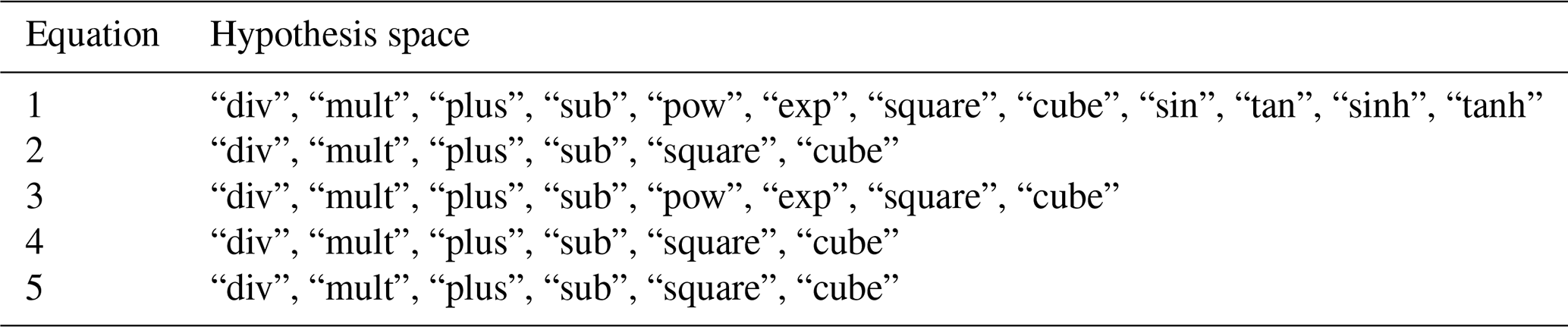
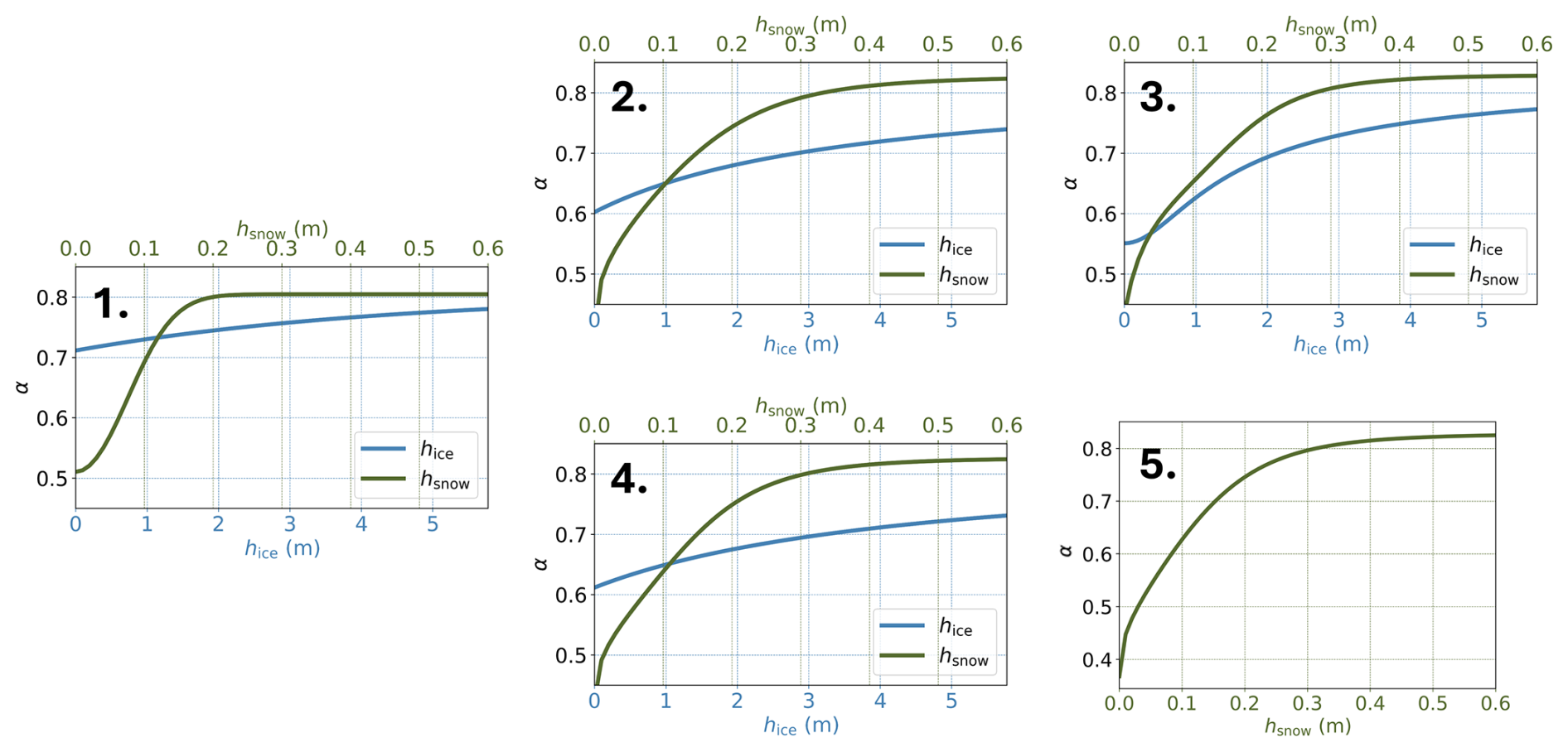
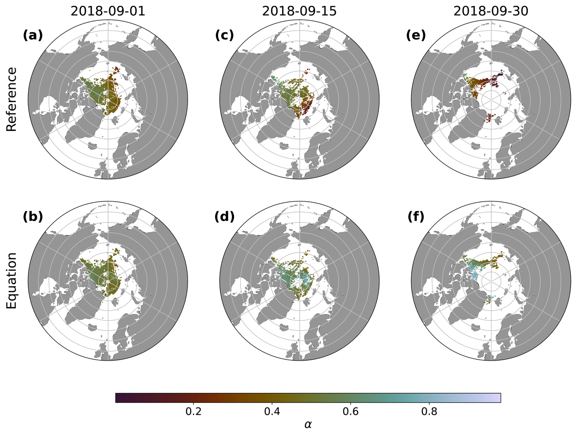
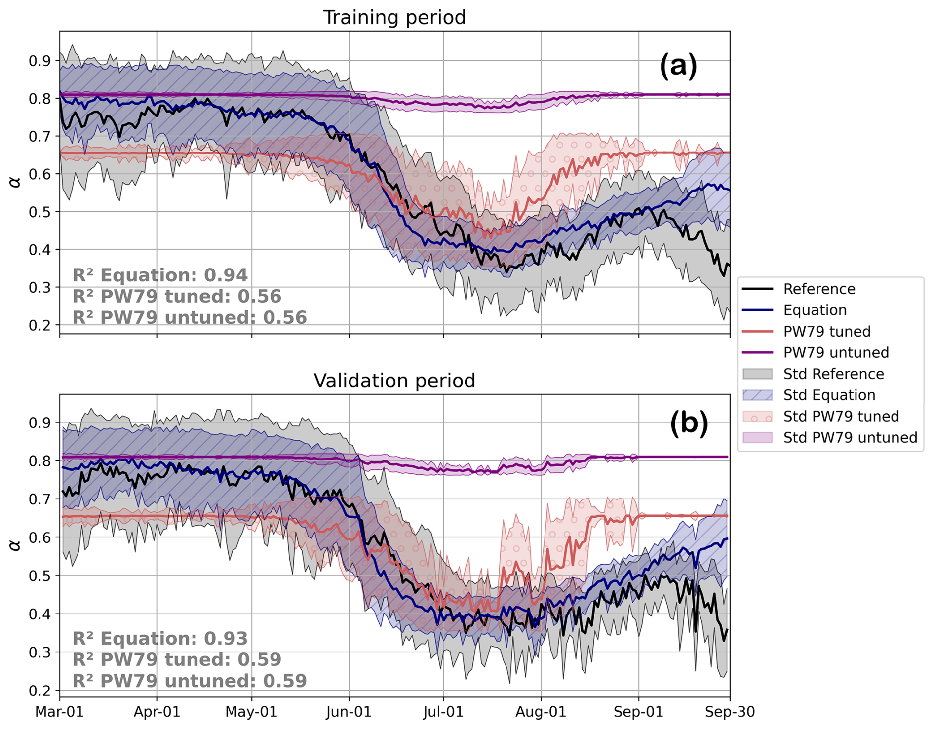
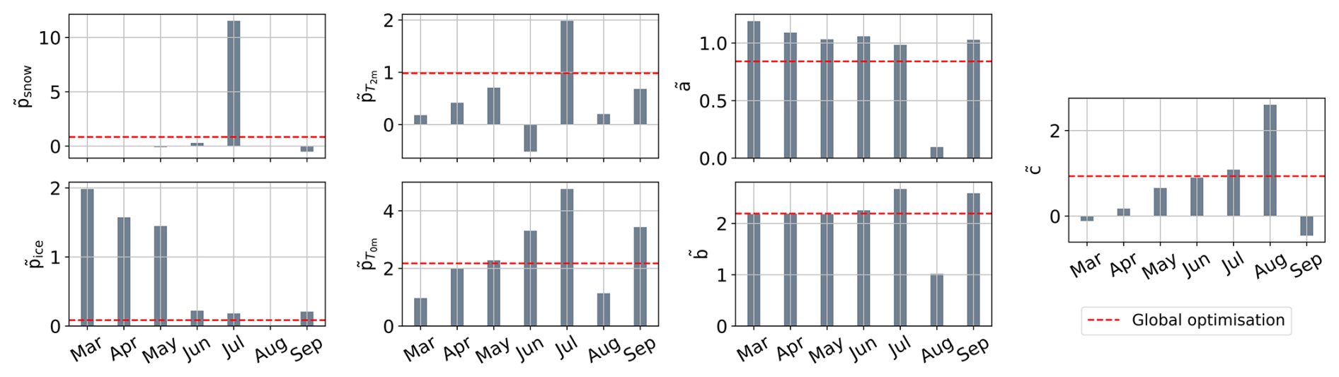
Figure G1 displays the regionally optimised coefficients in their unitless form using the BFGS-optimiser which we plug in to Eq. (4) to compute the MSE on the validation set shown in Sect. 5, Fig. 10.

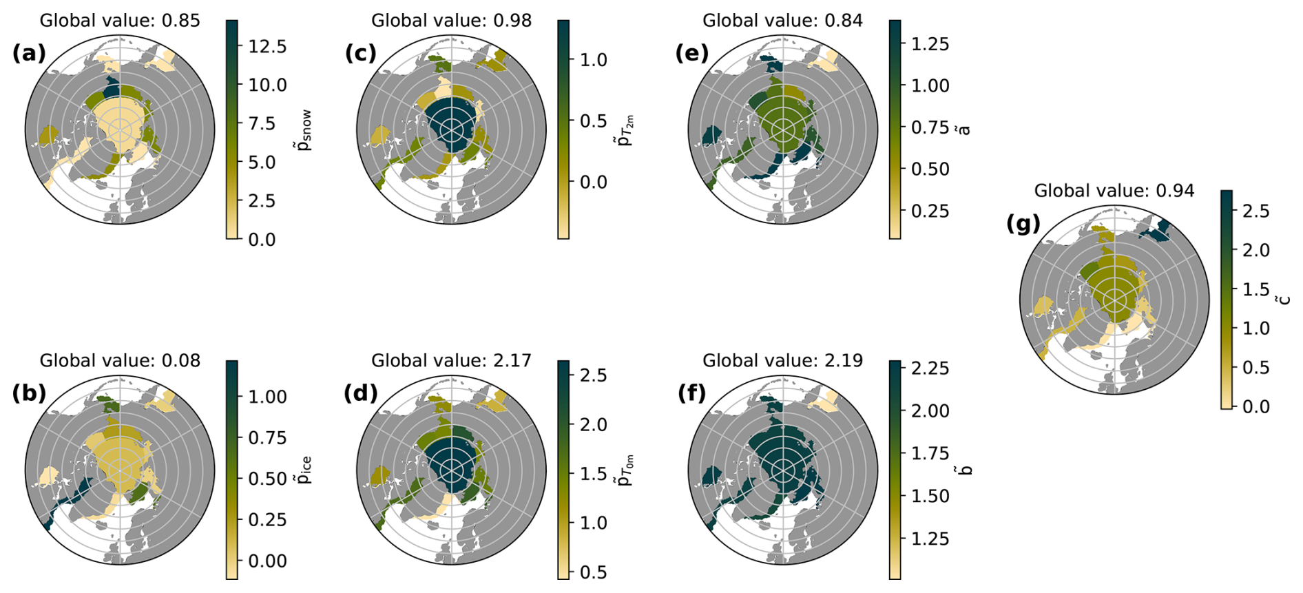
Figure G1 Regionally optimised coefficients of Eq. (4). The coefficients are unitless, meaning that they are rescaled by dividing by their standard deviations of the training set (2013–2018).

Appendix H: Monthly optimisation

Figure H1 displays the regionally optimised coefficients using the BFGS-optimiser which we plug in to Eq. (4) to compute the MSE on the validation set shown in Sect. 5, Fig. 10.

Figure H1 Monthly optimised coefficients of Eq. (4). The coefficients are unitless, meaning that they are rescaled by dividing by their standard deviations of the training set (2013–2018).