Uncertainty of the satellite-retrieved sea-ice area record and its trend

This study quantifies uncertainties of the observed Arctic and Antarctic Sea-Ice Area (SIA). Uncertainties in SIA estimates are derived from a single product, using a refined method to propagate local sea-ice concentration (SIC) uncertainties to hemispheric SIA estimates. The method accounts for spatial and temporal error correlations. The SIA uncertainty time-series based on the EUMETSAT Ocean and Sea Ice Satellite Application Facility (OSI SAF) SIC record is relatively stable over time, even though SIA itself shows notable seasonal and long-term variability. The seasonal cycle of the uncertainty is instead linked largely to the distribution of the ice. In the growing season, the SIC fields are more compact with a shorter sea-ice edge separating high and low sea ice concentrations. In the melting season the sea-ice edge is in comparison more diffuse. This seasonal evolution of the sea-ice edge leads to a relatively large SIA uncertainty in the melting season and a smaller uncertainty in the growing season.

The new single-product time series is compared with the spread across several SIA satellite products. The spread in the latter is characterized by seasonally varying biases. After accounting for these biases, the remaining differences are consistent with our new single-product SIA uncertainty. The two approaches are complementary: The inter-product approach provides insights into the influence of the product development while the new single-product SIA uncertainty allows for dynamic daily and monthly estimates which do not rely on the selection and availability of other products. It represents the non-systematic (bias-free) component of the uncertainties, which, among other things, determines the significance of new SIA extremes.

The single-product, non-systematic uncertainties in SIA trends from 1979 to 2025 are estimated to be 11⋅10³ km² per decade (Arctic) and 14⋅10³ km² per decade (Antarctic). Our analysis shows that systematic uncertainties are present in the SIA trend estimates. This indicates that a longer time-series will not be sufficient to remove trend uncertainties. For an extensive uncertainty quantification, systematic uncertainties should be represented explicitly. These uncertainties are related to methodological choices in the SIC product development, such as the homogenization across passive microwave sensors, applied masks, corrections and interpolations. The respective influence of these choices on SIA trend observations requires further research.

1 Introduction

Uncertainties in observations of Sea-Ice Area (SIA; the sum of all grid cell surface areas multiplied by their Sea-Ice Concentrations, SIC, per hemisphere) are critical because they directly impact the accuracy of assessing the state and long-term trends in the polar climate system. Reliable data are essential for evaluating and improving climate models, which depend on precise measurements and robust observational uncertainty estimates. Uncertainty estimates of the sea-ice indicators create reliability and confidence in climate assessments, which support informed policy decisions (von Schuckmann et al., 2026). Overall, quantifying uncertainties enhances our confidence in scientific conclusions, which makes it surprising that relatively little is known about the uncertainties in satellite-derived estimates of SIA and SIA-trends. To overcome this, this study quantifies the uncertainty of SIA, retrieved for the whole passive microwave satellite record, and furthers our understanding of the types and sources of SIA and SIA-trend uncertainties.

Uncertainties of the SIA observations are much smaller than the observed changes, but the uncertainties have the potential to mask links to the climate system, disguising our view on factors driving SIA variability and potential changes in the system. Another line of investigation of the polar system are modelling studies. Those models, including climate models, are often evaluated against their ability to reproduce the observed changes in sea ice cover (SIMIP Community, 2020; Roach et al., 2020). It is essential to consider observational uncertainties in these evaluations to avoid unjustifiably harsh penalties.

The required uncertainty estimates of passive microwave SIA and Sea-Ice Extent (SIE, the sum of the area of all grid cells with SIC > 15 %, per hemisphere) time series are so far either based on individual case studies (Meier and Stewart, 2019) or the spread between different SIC products (SIMIP Community, 2020; Roach et al., 2020; Kern et al., 2019; Ivanova et al., 2014; Meier et al., 2022). Those comparisons show clear biases between the products which cannot be fully explained by the use of different land masks or resolution (Kern et al., 2019). Another limitation of this approach is that many products use at least in parts the same underlying measurements and methodologies, so that the number of independent SIA and SIE products is even smaller than the number of published products. Estimates from products with common approaches tend to behave more similar (Kern et al., 2019, 2020).

For the correct handling of uncertainties it is essential to separate their systematic components, such as biases, from their random, stochastic components. If knowledge of the absolute SIA is required, biases are relevant and primarily the large systematic uncertainties must be considered. In many cases relative SIA estimates are used, such as for correlation analysis or the ranking of sea ice minima. In these cases uncertainties from inter-product comparisons, including systematic uncertainties, would lead to a strong overestimation of uncertainty.

We address the problem of separating systematic and stochastic uncertainties with the help of a new approach to quantify stochastic SIA uncertainty from Wernecke et al. (2024). This approach relies on the local SIC uncertainty estimates in the OSI SAF SIC product, which are one of the most mature uncertainty estimates for passive microwave SIC products. These SIC uncertainties are propagated to the aggregated measure of SIA, following Wernecke et al. (2024). This approach, in its refined version described in Sect. 2.1, has been developed to support the OSI SAF Sea-Ice Index (SII) with uncertainty estimates. Here we give a first overview of these uncertainty estimates over the full time series and across the seasons. We investigate the origin of the uncertainty seasonality in Sect. 2.2. The consistency of the single-product uncertainty with the SIA from other Sea Ice Concentration data-sets is investigated in Sect. 3 and the role of systematic SIC uncertainties on trends in SIA is addressed in Sect. 4. Section 5 discusses amongst other things which uncertainty components are represented by each of the approaches.

2 The Uncertainty Record

In the following we first give a general overview of our methodology, followed by processing details specific to the new uncertainty time series. In doing so, we focus on the SIA as our main metric of interest, and thus do not cover issues arising from the non-linearity and the grid-dependence of the alternative metric Sea-Ice Extent (Notz, 2014).

2.1 Processing

Overall, our processing closely follows the one described by Wernecke et al. (2024). We first briefly outline its basis, before highlighting some refinements introduced for the present work.

In Wernecke et al. (2024), SIA uncertainties are propagated from local uncertainty estimates of the OSI SAF SIC product under consideration of spatial and temporal SIC error correlations. We use the Climate Data Record (CDR) OSI-450-a1 (EUMETSAT OSI SAF, 2022a) extended by the interim CDR OSI-430-a (EUMETSAT OSI SAF, 2022b). The approach is fully reliant on the SIC uncertainty component which we do not attempt to verify or improve here. A comprehensive validation of the CDR has been performed in Kreiner et al. (2022).

The OSI SAF SIC uncertainty variable total_uncertainty used here is the quadratic sum of two components: (1) the algorithm_uncertainty, which accounts for sensor noise and residual geophysical variability derived from the algorithm performance over open-water and consolidated-ice training data. And (2) the smearing_uncertainty, which represents mismatches between sensor footprints and the target grid as well as differing channel fields of view. Smearing uncertainty is strongest in regions with sharp SIC gradients and is parametrized as a function of the local SIC range within a 3 × 3 neighbourhood, with the proportionality factor calibrated using MODIS-based (optical) footprint simulations (Lavergne et al., 2019). The total_uncertainty field, along with its algorithmic and smearing components, is provided with the OSI SAF SIC product.

The uncertainty propagation makes use of a Monte-Carlo (MC) approach which relies on a stochastic representation of the SIC uncertainties to generate an ensemble of daily SIC maps. The spread between SIC ensemble members represents the SIC uncertainty which translates into the SIA uncertainty when we derive the corresponding ensemble of SIA time series and analyse its spread. The processing is performed on daily data from a given month at a time and involves the following steps: (1) create a spatio-temporal field of noise with radially declining autocorrelation in space and time, (2) normalize the amplitude of that field to a standard deviation of one and multiply with the OSI SAF total_uncertainty variable, (3) add the scaled noise to daily SIC fields, (4) derive the daily and monthly mean SIA for this ensemble member and (5) repeat from step (1) until the desired number of ensemble members is reached (here: 50 members).

The SIC error correlation characteristics used in step (1) are crucial to link SIC uncertainties to SIA uncertainties. Yet, they are not well known. Wernecke et al. (2024) and Kern (2021) derive estimates by selecting areas and times where it is assumed that the real SIC is close to 100 % so that the corresponding fluctuations around 100 % of the SIC product are understood as errors from which the temporal and spatial correlation length scales can be derived. These length scales are used to set up a Gauss-filter which is applied to fields of random independent noise to create radially correlated noise for step (1). This noise is scaled by the total_uncertainty variable in step (2) and added to the smoothed OSI SAF SIC field. The smoothing is performed with the same Gauss-filter as before on the un-truncated (not restricted to values between 0 % and 100 %) OSI SAF SIC to remove high frequency fluctuations. This is an attempt to replace the errors inherent in the SIC dataset by synthetic realizations in step (3). These sample can then be used (step (4)) to calculate the SIA (or SIE). The spread in the SIA ensemble (created by repeating steps (1) to (4)) represents the corresponding uncertainties. The SIC ensemble members generated in step (3) are tested to reproduce the initial estimates of SIC error correlations.

Since we focus on uncertainty estimates of daily and monthly-mean SIA observations (no yearly-means) we can process each month separately. In general the MC ensemble is used for estimating the uncertainty (ensemble spread) but where we show absolute SIA values we use the original OSI SAF SIC for calculation instead of (e.g.) the mean of the ensemble to ensure consistency.

For the scope of our study, we introduce three modifications to the general workflow from Wernecke et al. (2024). These are (a) the interpolation of SIC uncertainties for missing data, (b) the consideration of land-spill over corrections, and (c) our handling of SIC values filtered by the weather filter:

SIC uncertainty interpolation

The CDR SIC processing (OSI-450-a1 and OSI-430-a) includes temporal and spatial interpolation of SIC to fill data gaps and provide a more complete data record. No local SIC uncertainties are provided for these interpolated locations which we now fill in to avoid providing an incomplete picture of the SIA uncertainties. To first order, the SIC uncertainty can be expressed as a function of the SIC value itself, accounting for the fact that OSI SAF SIC uncertainties are mostly small at concentrations near 100 % and near 0 % and largest in the intermediate range (including the Marginal Ice Zone). This inspired the following gap filling approach: For each daily SIC file we bin all the SIC values in ranges below 0  %, above 100 % and each interval of 10  % in between. The uncertainty in each interpolated SIC location is set to be the median uncertainty of the corresponding SIC bin. In this way each location with an interpolated SIC value is assigned an uncertainty value typical for its range. This approach is not accounting for uncertainties from interpolation itself.

Handling of land spillover

In general, we start the processing with the “raw” OSI SAF SIC product. Its values are un-truncated to make sure that no additional bias is introduced. This is important especially at 100 % SIC, where truncation is removing positive errors but retaining negative errors. The difference to Wernecke et al. (2024) is that here we apply the land spill-over correction to the “raw” SIC product. The land spill-over correction is designed to reduce a known positive bias in coastal SIC caused by land contamination of coastal passive microwave measurements (Lavergne et al., 2019). There is no reason not to apply this correction in our processing, which is also more consistent with the current Sea-Ice Index processing.

The weather filter

Weather affects the ocean surface, in particular in regions without sea ice, which can cause the SIC algorithm to produce values above 0 %. The weather filter (also referred to as open water filter) removes this spurious SIC values (setting SIC to 0 %) where the Brightness Temperature signature indicates the influence of weather on the SIC algorithm (Lavergne et al., 2019). Here the filter is applied to the background SIC (after the Gauss-filter is applied, see above) before the error realizations are added. This makes our uncertainty processing more consistent to the Sea-Ice Index processing where the weather filter is also applied, but introduces potentially new errors if weather effects are erroneously flagged. To account for these new errors, we keep the local SIC uncertainty values for regions where the weather filter has removed potential sea ice. For the same reasons as stated before, SIC realizations are not truncated and can also become negative. Therefore changes to the background field have no impact on the SIA uncertainty, but would have an impact on the SIE uncertainty.

2.2 Evolution of the SIA uncertainty

We create a synthetic Monte-Carlo ensemble of SIC fields with 50 members, and then calculate the monthly SIA for each of these fields. The observational uncertainty is represented by the spread in the SIA ensemble for which we often use the standard deviation as measure. When deriving SIA standard deviations we can expect the estimate to be within 10 % ($\frac{\mathrm{1}}{\sqrt{\mathrm{2}N}}$ with N=50 being the sample size) of the population standard deviation. The population standard deviation is the analytical value of a distribution to which estimates converge with increasing sample size. This estimation uncertainty is reduced further for averages over the record or if running means are applied (Fig. 1).

There is a seasonal cycle in the SIA uncertainty (Fig. 1a) which shows smaller uncertainties around, or a few months past, the respective SIA minima in February for the Antarctic and in September for the Arctic (Fig. 1b). While the amplitude of the uncertainty seasonal cycle is relatively weak compared to that of the SIA (Fig. 1b), it explains more than half of the total variability over time of our uncertainty time series (Fig. 1a, c, d).

The monthly ensemble uncertainty (one standard deviation) in Arctic SIA is between 0.09⋅10⁶ km² (October) and 0.12⋅10⁶ km² (June) (average: 0.10⋅10⁶ km²). The monthly Antarctic SIA ensemble uncertainty is between 0.10⋅10⁶ km² (March) and 0.15⋅10⁶ km² (December) (average: 0.13⋅10⁶ km²) (Fig. 1a).

Overall, there is little change over time in the SIA uncertainty record (Fig. 1c,d) with slightly larger, and more variable uncertainties in the south than in the north (Fig. 1a). In particular, there is no noticeable increase in monthly SIA uncertainties before 1987, where SIC data exists only for every other day. This is consistent with the temporal error auto-correlation of about 5 d (Wernecke et al., 2024), which means that there is hardly any additional cancellation of errors when calculating the monthly mean SIA from the SIC sampled at a daily frequency, instead of at alternating days. In other words, the added value of daily SIC fields for monthly mean SIA estimates is very limited. There is no clear trend in the monthly SIA uncertainty over the record which indicates that the sensor performance (which improved over time) is not a critical factor for the SIA uncertainty and that the inter-sensor calibration of the passive microwave fundamental climate data record (Fennig et al., 2020) might have minimized spurious variability in the SIC record. A major component of the SIC uncertainty is the so called smearing uncertainty, which is caused by variability in the SIC and can primarily be improved by higher resolution. This is also why the Monte-Carlo SIA uncertainties based on the 25 km SIC product are smaller than for the companion product with 50 km resolution (not shown).

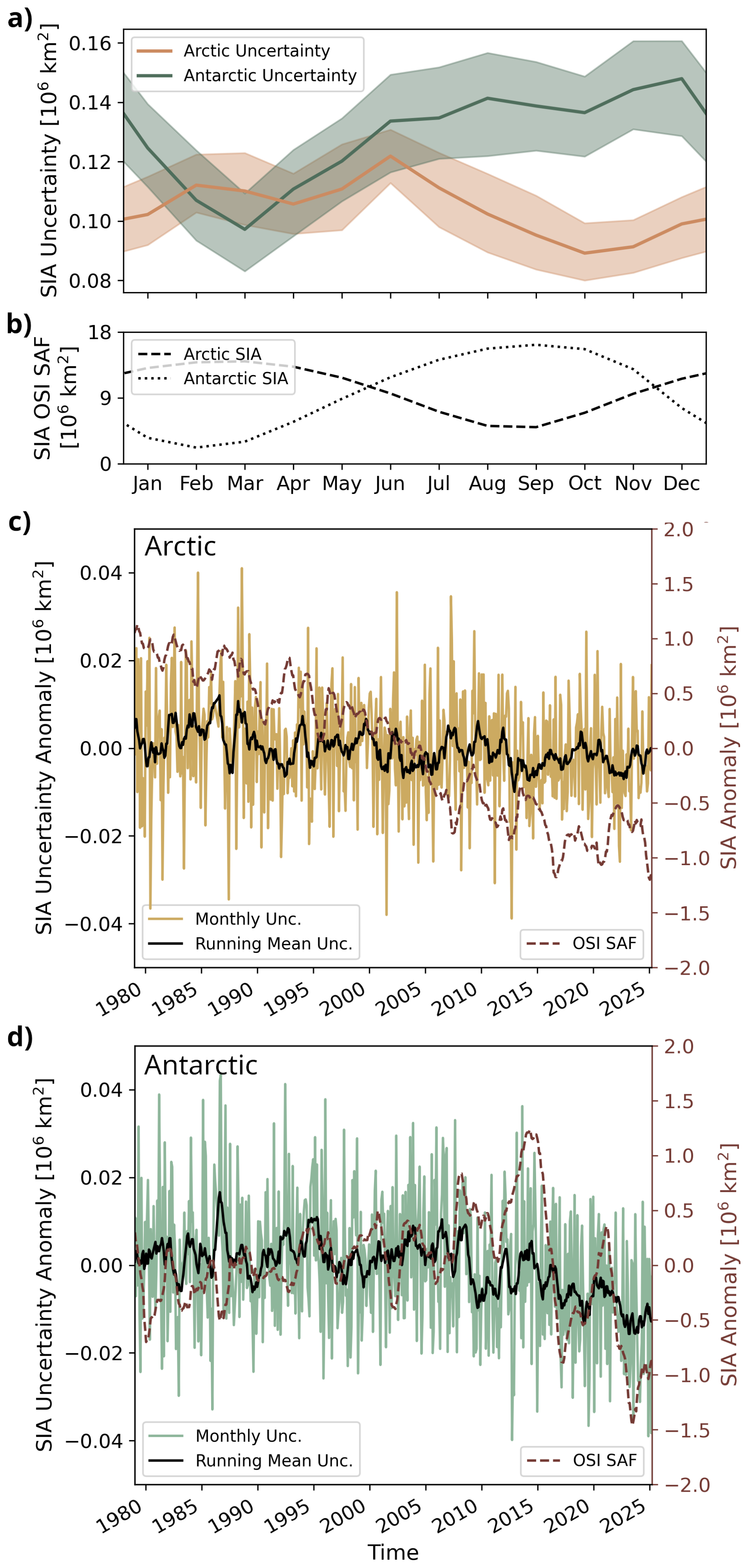
Figure 1 Evolution of our SIA uncertainty (one standard deviation of the ensemble). (a) Seasonal cycle of the ensemble uncertainty with 68 % frequency interval over the record (shades), (b) OSI SAF SIA seasonal cycle for comparison, (c) Arctic, and (d) Antarctic monthly ensemble uncertainty anomaly (seasonal cycle removed) with 12 month running mean on the monthly uncertainties (black line) and OSI SAF SIA anomaly for comparison (dashed line). Only months with at least 10 daily estimates are included.

We also derive the regional SIA uncertainties for which we use the predefined regions from Meier and Stewart (2023). Following our expectations, regions with small SIA tend to have relatively large uncertainties (a poor signal to noise ratio). More on regional uncertainties can be found in Sect. S1 of the Supplement.

Generally one would expect the SIA uncertainty to be larger for larger SIA values since more non-zero SIC grid cells are summed up. More specifically the uncertainty of a sum increases with the square-root of the number of independent summands. While there is a small decrease in Antarctic SIA uncertainty past the 2015/2016 SIA decline, generally the changes in SIA uncertainty and its seasonal cycle (Fig. 1a, c, d) are much smaller than the changes in SIA itself and its seasonal cycle (Fig. 1b and dashed lines in Fig. 1c, d). This poses the question as to why periods with larger SIA often do not show larger SIA uncertainties (Fig. 2a, b).

Figure 2c,d show that the SIA uncertainty is clearly related to the square-root of the length of the sea-ice edge which we derive here as a 50 % contour of the 25 km resolution SIC product. We sum the total length of this contour without constraining the water side to be connected to the open ocean (ocean to land or ice to land interfaces are not included). The important role of the sea-ice edge for the SIA uncertainty can be explained by the fact that the OSI SAF SIC uncertainties are much larger in regions with high SIC gradients (driving the smearing uncertainty) and those gradients are much higher at the sea-ice edge, which behaves very different to the SIA over the year (Horvat, 2021, Sect. S2 in the Supplement).

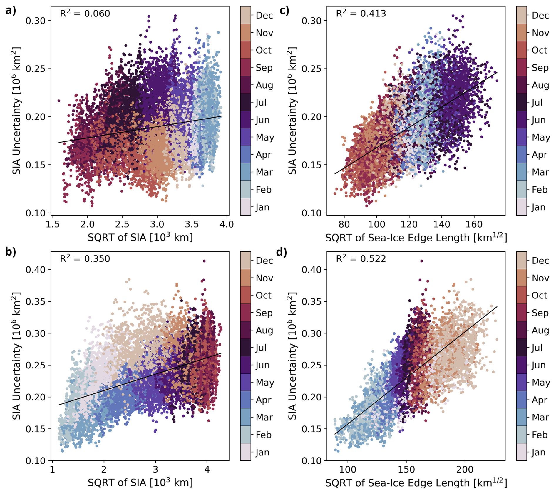
Figure 2 Relation of the SIA uncertainty to the square root of the SIA (left) and square root of the length of the sea-ice edge (right) defined here as the length of a 50 % SIC contour line for the northern (top) and southern (bottom) hemisphere. Each dot represents one month of the full time series (1979–2025), with squared correlation coefficients, R², in each panel.

3 Consistency with inter-product estimates: SIA

Uncertainties in observational SIA are traditionally estimated by calculating the differences across different satellite products (e.g. Roach et al., 2020; SIMIP Community, 2020). Meier and Stewart (2019) find SIE uncertainties from algorithm parameters and input source data around 30 000 and 70 000 km² which is smaller than the difference between near-real-time and final product processing at the National Snow and Ice Data Center (NSIDC) (around 100 000 km²). But how do our new estimates compare to inter-product SIA uncertainties? For this comparison we use SIA time series, processed consistently at the University of Hamburg (Rauschenbach et al., 2024), extended to the end of 2024 by Thomae et al. (2025) (hereafter called UHH product). The UHH SIA product is based on six SIC products, namely the HadISST SIC products in original and NSIDC configuration (ending mid 2020), the OSI SAF SIC product, the Bootstrap and NASA Team products (CDR version 4.0) and the Climate Change Initiative (CCI) product (starting in 1991). Note that some of these estimates are relatively similar in nature, in particular the two HadISST products as well as the OSI SAF and CCI products. As a compromise in length of time series and number of products we include the HadISST products in this chapter but exclude the CCI product, resulting in five products from 1979 to 2020.

Figure 3 Arctic (a, c) and Antarctic (b, d) SIA time series (top) and year to year SIA distributions (bottom) based on six SIC products, for the period from 1979–2020 where five products are available from Thomae et al. (2025). For the distributions (b, d) the product mean SIA time series is subtracted but inter-product biases included (dark purple) or with individual product means removed (light purple). The white bar is purely based on the SIA uncertainty ensemble distribution introduced here showing the average ensemble spread of each month. Whiskers enclose the 5 to 95 percentile range, horizontal lines show the median.

As can be seen in Fig. 3, the products differ in SIA in the order of one million km², depending on the hemisphere and time of the year. The inter-product spread is about as large, or even larger, as the temporal variability visible in Fig. 3a, c. The well-known systematic biases between the time series (e.g. Ivanova et al., 2014; Kern et al., 2019) clearly show up by their largely parallel, but distinct temporal evolution.

By construction the single-product uncertainty that we estimate in the previous section, cannot represent systematic uncertainties, so that a meaningful comparison must focus on the consistency of our uncertainty estimate with the spread across different SIA products after their systematic biases have been removed. To remove the systematic biases, we separate the time series by month of the year (removing the impact of the seasonal cycle) and subtract the multi product mean SIA (removing the impact from climate variability). The resulting distribution for all years and products is shown in Fig. 3b, d as dark purple boxes. As mentioned before, most of this spread is caused by biases between the products, which are removed as a next step by subtracting the mean of each product's distribution before combining them (light purple boxes in Fig. 3b, d). For comparison the distribution of the ensemble presented here is illustrated with the ensemble mean removed in white in Fig. 3b, d. The effect of the large inter-product bias is clearly visible in the large difference between the light and dark purple bars of Fig. 3b, d. The agreement in width of the bias-free inter-product distribution and the single product MC ensemble (white boxes in Fig. 3b, d) is remarkable with the inter-product spread being about the same as the single product estimate throughout the year.

We want to highlight the very different origins of the two uncertainty estimates: The sample uncertainty originates on the OSI SAF SIC uncertainty product alone which is not directly linked to any decisions in the processing. The inter-product uncertainties shown in Fig. 3b, d represent a combination of effects from algorithms and sensors/frequencies used. A more detailed discussion of the represented uncertainties is given in Sect. 5. The general agreement between the estimates supports our confidence in the proposed uncertainty estimates.

4 Consistency with inter-product estimates: SIA Trends

We further compare the uncertainties in trends between our single-product ensemble approach and the UHH SIA multi-product comparison. The spread in trends is represented in Fig. 4 by the width of gray distributions and compared with the trends in the UHH product for March and September estimates. For the trend analysis it is much more important, that the time-series are up-to-date and at maximal length, which is why the HadISST products are excluded. This leaves the OSI SAF, NASA Bootstrap and NASA Team products for the period of 1979 to the end of 2024. However, the conclusions remain the same for the shorter time-period including HadISST (not shown).

Figure 4 SIA trend estimates for 1979 to 2024 (inclusive) based on Thomae et al. (2025) (coloured lines) and probability distributions of our ensemble estimate (gray), centred on the OSI SAF estimate. Shown are the March and September trend estimates for the Arctic (a) and Antarctic (b). Other months are shown in Sect. S3 of the Supplement.

It is striking that the trends across different products vary widely, often considerably more than the ensemble uncertainty (Fig. 4). This indicates that also the trends are affected by systematic uncertainties from the processing, that are not represented in the ensemble uncertainty. The fact that the ensemble distribution in Fig. 4 is (by construction) centred on the OSI SAF estimate does not indicate that it is closer to reality. Instead Fig. 4 simply shows that the differences in trend estimates of different products cannot be explained by stochastic OSI SAF uncertainties.

The ensemble Arctic SIA trend uncertainty (one standard deviation) is between 9⋅10³ and 13⋅10³ km² per decade (average: 11⋅10³ km² per decade). Antarctic ensemble SIA trend uncertainty is between 10⋅10³ and 18⋅10³ km² per decade (average: 14⋅10³ km² per decade). The trend uncertainty for September in Antarctica is larger than for March or the Arctic trends shown in Fig. 4, which is consistent the average Antarctic September SIA uncertainty being the largest of the four month/hemisphere combinations shown here (Fig. 1a). While the small sample size of the inter-product approach does not allow for robust estimates of an inter-product standard deviation, it is clear, that the inter-product spread is substantially larger than the ensemble spread (see also Sect. S3 of the Supplement).

5 Discussion

We introduce an uncertainty estimate for the Arctic and Antarctic SIA over the full passive microwave SIC period and analyze its variability, origin and the consistency with other uncertainty estimates. The SIA uncertainty estimate itself relies on the uncertainty estimate of the foundational OSI SAF SIC product together with the refined method of Wernecke et al. (2024). If the OSI SAF SIC uncertainties are overestimated or underestimated, this will also manifest in the SIA uncertainties presented here. We carried out a related sensitivity analysis and found that SIA uncertainty is linearly related to the absolute amount of SIC uncertainty (Supplement Sect. S4). This approach is complementing traditional inter-product uncertainty estimates and hence provides new insights into the crucial SIA uncertainty.

5.1 Systematic and stochastic uncertainties

The SIA products are known to have substantial biases (e.g. Fig. 3) indicating systematic uncertainties, which are discussed in much more detail in the literature (e.g. Ivanova et al., 2014; Kern et al., 2019; Meier et al., 2022). These biases can be explained by a combination of resolution, projection, land masks, the signal contamination from nearby landmasses, filling of the polar hole in observations, dynamic tuning of the algorithms, filters applied, but also how the algorithms handle surface and atmospheric emissivity variations (Kern et al., 2019, 2020; Ivanova et al., 2014; Meier et al., 2022). Another source of systematic uncertainties in SIA during summer months are the challenges for passive microwave SIC algorithms posed by snow melt, refreeze processes, and the presence of melt ponds (Kern et al., 2020; Alekseeva et al., 2019). These challenges are only partially represented by the OSI SAF SIC uncertainty estimate (Kern et al., 2020).

Stochastic uncertainties include independent errors and errors correlated locally in space and time (on the order of hundreds of km and weeks, or smaller). This includes sensor noise, but also undesired effects of varying snow, ice, ocean and atmospheric properties as well as gridding effects, which are discussed below.

Whether the stochastic component or the systematic component (including biases) is more relevant for an application depends on the subject. If knowledge of the absolute SIA is required, biases are relevant and the large uncertainties as e.g. shown in Fig. 3b, d in dark purple have to be considered. The assessment of climate models would fall into this category, even though we would recommend to derive the SIA from SIC on the model grid, to avoid the influence of the e.g. different land masks. In other words, a climate model should be judged by its ability to produce realistic amounts of sea ice in its own domain, not in parts of the reality which it does not resolve. For other applications relative changes in SIA are more relevant such that stochastic uncertainties become decisive. Examples would be investigations of the correlation of (regional) sea ice cover variability with climate indices or the identification of a new sea ice minimum. In both cases biases are not relevant and using the full inter-product spread in SIA products would be a strong overestimation of uncertainty.

5.2 Uncertainty components represented by each approach

In this section we discuss which aspects of the SIA estimation are represented by the uncertainty estimates. This provides context for the presented values, guidance on the application of these uncertainties and motivates further research on SIC/SIA uncertainties.

The new MC single-product approach represents errors caused by gridding and the combination of measurements with different footprints. The OSI SAF SIC uncertainty includes the smearing_uncertainty variable which is based on the local gradients in SIC because measurements within fields of large gradients are more sensitive to the exact location of the measurements (Lavergne et al., 2019). In contrast, the inter-product approach covers these uncertainties only in cases where the products use different grids for the final SIC maps, or internally for the pre-processing and processing steps. This indicates that gridding uncertainties are under-sampled in the inter-product estimates, in particular where products are processed in a similar way (ESA-CCI and OSI SAF, NASA-Team and Bootstrap, or the two HadISST product versions).

The OSI SAF SIC uncertainty also includes a variable called algorithmic_uncertainty which is based on the variability of measurements within the tie-points. Tie-points are measurements corresponding to 0 % and 100 % SIC, which are used to calibrate all other measurements. OSI SAF uses dynamic tie-points based on a first guess SIC estimate together with geographic masks, numerical weather predictions and radiative transfer correction to cluster open-water and sea-ice reference measurements (Lavergne et al., 2019). The algorithmic_uncertainty can be interpreted as a measure of two effects: (a) uncertainties in how well the tie-point signature is known (which is a spatially correlated error effecting all SIC measurements with the respective ice type), and (b) the noise-level in this groups of measurements which have, by design, a very homogeneous sea ice cover (either close to 0 % or close to 100 %). Therefore the algorithmic_uncertainty also represents the noise of repeated measurements of 0 % and 100 % sea ice, including the effects of sensor noise, atmospheric interference and local surface emissivities. The surface emissivity is in turn defined by snow and ice surface properties such as density, grain-size, grain-type and wetness variations for the ice tie-points, and ocean waves/ripples, foam and temperature for the ocean tie-points. Imperfections in the atmospheric correction of the OSI SAF SIC product further adds variability within the tie-points. Inter-product differences can be argued to represent some of such factors as well, though not in the same way: The products do often have different tie-point definitions with resulting variations in the reference values for deriving the SIC (comparable to component (a) above). Sensor noise or the effects of locally varying surface emissivity (component (b) from above) would only be represented in rare cases where the SIC products do not use the same measurements, such as products based on 89GHz channels (e.g. Spreen et al., 2008) (not used here). Ultimately some products are more conservative in the tie-point definition than others, which can cause a shift in the calibration and create systematic differences in SIC. Different atmospheric corrections schemes are applied between the products, leading to a representation of the corresponding effects in the inter-product uncertainty estimates.

Overall the MC SIA uncertainties are based on OSI SAF SIC uncertainties which have a much clearer definition of what they represent: Errors in tie-point estimates, noise in measurements near 0 % and 100 % SIC, and effects from measurement mismatches and gridding. The inter-product approach covers some of the same aspects, but gives a much more fractured estimate which also depends on which products are used. The advantage of the inter-product approach is, that some uncertainties from the SIC product development are currently not, or only partly included in SIC uncertainties, such as uncertainties from applied corrections, masks, interpolation or melt ponds.

5.3 Seasonality and trend uncertainties

We have found that the SIA uncertainty is to a good extent driven by the sea-ice edge, which is also consistent with the finding that the SIA uncertainty is largest in December (Antarctica) and June (Arctic) (Fig. 1a), i.e. later in the year than the corresponding yearly peaks in SIA. This is because the sea-ice cover is more diffuse when retreating, compared to a more compact distribution when advancing leading typically to a longer sea-ice edge in spring than in autumn (Sect. S2 in the Supplement).

The evolution of Sea Ice Area over time is not necessarily well represented by a linear trend. This is particular true for the Southern Ocean where sudden and drastic changes in SIA are observed around 2015/2016 (Fig. 1d). Nevertheless, linear trends find considerable attention in literature for both hemispheres (e.g. Roach et al., 2020; Shen et al., 2021; Meier et al., 2022). While we recognise, that the SIA trend is not the only measure of the sea ice cover change, we use it here for consistency.

Antarctic SIA trends are much smaller than Arctic trends, and while the inter-product spread of the trends might be consistent with the ensemble spread in March, the two estimates do not agree for most other months of the year, including September (Fig. 4b, Sect. S3 in the Supplement). As mentioned, there are only three SIA products which cover the whole period and it is possible that in March they fall unusually close to each other simply by chance. In fact the inter-product spread increases substantially if HadISST is included (for 1979–2020) (not shown).

Trends in SIA and SIE are compared in Meier et al. (2022) based on the NOAA/NSIDC Climate Data Record (CDR) Version 4 with the NASA Team (NT) and Bootstrap (BT) products. Despite the fact that the CDR is a combination of the other two products and in particular very similar to the BT product, Meier et al. (2022) calculate the differences between the products and these differences have statistically significant trends, supporting the presence of systematic uncertainties. Differences between trend estimates are typically 10 % of the trend estimates themselves for the SIE and can reach more than 20 % for the SIA (NT – CDR in March) (Meier et al., 2022). Comiso et al. (2017) derive SIA and SIE trends for four SIC products and report a spread in SIA trend estimates of about 50⋅10³ km² per decade for trends just above 500⋅10³ km² per decade which is a ratio consistent with Meier et al. (2022).

Ivanova et al. (2014) harmonize the processing of SIA estimates from different SIC algorithms by applying the same weather filter, surface temperature estimates (where required by the algorithms), open-ocean and land-ocean spillover masks to focus on the effects of the algorithms themselves. The very good agreement between trends for the 1979–2012 period in Ivanova et al. (2014) is therefore not contradicting the importance of systematic uncertainties in trends. Note also the large range in trend estimates for the shorter period 1992–2012, which includes six additional higher frequency products (annual mean trends of 0.766–0.978 million km² per decade; Table VI in Ivanova et al., 2014). Therefore the good agreement in 1979–2012 trends in Ivanova et al. (2014) cannot be interpreted in a way that the real trend in Arctic SIA since 1979 is known well enough for every application (e.g. Chevallier et al., 2017). That being said, our results do not question in any way that the Arctic SIA has been significantly declining since 1979 thought the year (Fig. 4a, Supplement Fig. S4a).

The spread in SIA (and SIE, not shown) trend estimates from different SIC products is concerning. Note that all SIA products observe the same realization of the climate system over the same period, based largely on the same measurements and approaches. This is why we consider a 10 % spread relative to the Arctic trend signal as substantial. We have shown that this inter-product spread is likely driven by systematic uncertainties, meaning that more measurements do not necessarily reduce the spread in estimates. Systematic uncertainties can create errors with the same structure as the quantity of interest (here: linear trend) and can therefore perfectly mimic the signal in a time-series analysis. This is a general problem and motivates research into the measurement stability (Gobron et al., 2026). The length of the time series is often referenced as limitation for a precise estimate of the trend, however, methodological choices in the processing of the SIC and conversion to SIA appear to be at least an equally important factor.

6 Conclusions

In this study we have described developments in the methodology for the OSI SAF SIC to SIA uncertainty propagation, which is aimed at supporting the development for an uncertainty estimate delivered with the OSI SAF Sea-Ice Index. While the overall variability of SIA is notable, the associated uncertainties have remained relatively stable over time. Seasonal variations are tied to the ice distribution rather than the SIA seasonal cycle, where the sea-ice edge poses the largest challenges to passive-microwave based satellite estimates of the the Sea-Ice Area. The differences between SIA products can be explained by our new uncertainty estimates if the known inter-product biases are removed. We provide an overview of the sources of uncertainty which are represented by the estimate and contrast those between the more traditional inter-product approach and our single product time series. The comparison of our stochastic uncertainty estimates with those from the inter-product approach reveals systematic uncertainties in SIA trend estimates. These systematic trend uncertainties are crucial to consider since they do not necessarily reduce with length of the record. Systematic components, such as uncorrected long-therm drifts, are further inherently challenging to separate from trends in a time-series analysis. By quantification of the stochastic component, we are able to provide a well defined, dynamic and more nuanced picture of observed SIA and SIA-trend uncertainties.