PIXAL: a physics-inspired explainable machine learning architecture for Greenland ice albedo modeling

The Greenland ice sheet (GrIS) is a major contributor to global sea level rise. A significant portion of the GrIS' contribution can be attributed to increased ice surface melting, which is strongly controlled by ice albedo, a property that regulates the amount of absorbed solar radiation that leads to surface melting. Yet, we lack a comprehensive understanding of the complex and nonlinear relationships ice albedo has with its environment and is, therefore, often simplified or crudely parameterized in climate models. However, an accurate representation of future ice albedo evolution is essential for reducing uncertainties in sea level rise projections. This study presents PIXAL, a physics-inspired explainable machine learning architecture that significantly outperforms the Modèle Atmosphérique Régional (MAR), a state-of-the-art regional climate model, in modeling ice albedo on the southwestern GrIS. PIXAL is based on an Extreme Gradient Boosting (XGBoost) model and is trained on a suite of modeled topographic, atmospheric, radiative, and glaciologic variables from MAR to capture the complex and nonlinear relationships with ice albedo observations obtained from the Moderate Resolution Imaging Spectroradiometer (MODIS). Performance metrics show that PIXAL achieves an R² of 0.563, a structural similarity index measure (SSIM) of 0.620, a mean squared error (MSE) of 0.005, and a mean absolute percentage error (MAPE) of 14.699 %, compared to MAR's R² of 0.062, SSIM of 0.112, MSE of 0.032, and MAPE of 46.202 %. Explainable artificial intelligence analysis reveals that topographic features, specifically ice sheet surface height and slope, are important drivers of ice albedo variability due to their relationships with ice exposure duration and the effectiveness in accumulating meltwater and light-absorbing constituents (LACs) on flat ice surfaces. Near-surface air temperature and runoff further significantly impact ice albedo variability by affecting the ice metamorphic state and accumulation of meltwater and LACs. These findings highlight that understanding the complex physical processes underlying ice albedo variability is essential for accurate climate modeling and sea level rise predictions. PIXAL represents a crucial advancement in ice albedo modeling and paves the way for improved representation of ice sheets in Earth system models.

1 Introduction

A significant portion of the acceleration of the global mean sea level rise over the last few decades has been attributed to increased surface melting from the Greenland ice sheet (GrIS) (Aschwanden et al., 2019). Climate models project a contribution to global mean sea level rise of 9 to 18 cm from the GrIS by 2100 for the Shared Socioeconomic Pathway SSP5-8.5 (Fox-Kemper et al., 2021; Riahi et al., 2017). The large uncertainty in this projection contributes to the hindrance to accurate and effective mitigation of the implications of sea level change on coastal communities. A large portion of the uncertainty stems from an incomplete understanding of the physical processes that control ice surface melting on the GrIS and their linkages to atmospheric and oceanic processes (van den Broeke et al., 2017). Specifically, we lack an understanding of the spatiotemporal variability of ice albedo, which plays a crucial role in modulating ice surface melt processes (Antwerpen et al., 2022).

Ice is exposed on the GrIS during the summer melting season (June–August) when increased insolation and increased atmospheric temperature induce melting of the winter snowpack overlying the ice. Snow melt generally occurs in the ablation zone at lower elevations near the ice sheet margin. Here, the surface mass balance is negative, with the ablation of snow and ice (melting, evaporation, and sublimation) being larger than the accumulation (snowfall, rainfall, and refreezing), resulting in a net surface mass loss and potential exposure of the bare ice surface. Ice melt is strongly controlled by the broadband ice surface albedo, which represents the ratio of reflected (upward) solar radiation flux to incoming (downward) solar radiation flux, weighted by wavelength (visible to near-infrared). For ice, the broadband albedo ranges from ∼0.1 to ∼0.7 (Klein and Stroeve, 2002; Liang, 2001; Tedstone et al., 2020; Warren and Wiscombe, 1980; Wiscombe and Warren, 1980) while the typical albedo of snow is ∼0.7–0.8. The incoming solar radiation that is not reflected by the ice is, instead, absorbed. Because of its lower albedo, a considerably higher amount of incoming solar radiation can be absorbed by ice than by snow. The absorbed radiation heats the surface and shallow subsurface ice and snow layers and induces melting. Meltwater from snow and ice has a low albedo of ∼0.1 and when mixed with ice and snow therefore further decreases the albedo, promoting additional melting. This is referred to as the meltwater-albedo feedback (Stroeve, 2001). Under future, warmer atmospheric conditions, snowmelt over the GrIS is expected to increase (Yue et al., 2021). Therefore, the snowline is expected to retreat earlier and further inland, increasing the low-albedo ice areas and accelerating surface melting and sea level rise (Ryan et al., 2019).

Ice albedo on the GrIS is a highly complex property that is controlled by many factors. The metamorphic state of the surface and shallow subsurface of the ice, determined by ice grain size, density, porosity, specific surface area, and the size and shape of englacial air bubbles, plays a key role in the scattering, absorption, and reflectance of incoming solar radiation (Flanner and Zender, 2006). Moreover, meltwater and rainwater can pond on the ice surface and infiltrate shallow subsurface cavities in the ice, promoting absorption of incoming solar radiation during low cloud-cover days (Tedstone et al., 2020). Solar radiation heats the meltwater and promotes ice melting at the water-ice interface, increasing the presence of meltwater and further darkening the ice sheet. The presence of light-absorbing constituents (LACs), including black carbon, mineral dust, and algae can significantly lower ice albedo (Goelles and Bøggild, 2017; Hofer et al., 2017; MacGregor et al., 2020; McCutcheon et al., 2021; Williamson et al., 2020). A considerable fraction of LACs that affect GrIS ice albedo are aerosols from distant and local sources (Flanner et al., 2021; Goelles and Bøggild, 2017). Natural sources, including North American, Siberian, and Greenlandic wildfires, emit black carbon particles that have been found on the GrIS (Calì Quaglia et al., 2022; Keegan et al., 2014). Greenlandic wildfires can deposit up to 30 % of their emissions onto the ice sheet (Evangeliou et al., 2019). Asian and African deserts (Újvári et al., 2022), Icelandic volcanoes (Meinander et al., 2016; Moroni et al., 2018), and Greenlandic ice-free areas (Amino et al., 2021; Nagatsuka et al., 2021) also release dust particles that have been found on the ice sheet. Further, anthropogenic sources, including transportation, industrial, and residential, emit aerosols (Bond et al., 2013), which can be transported across large distances by atmospheric circulations and deposited on the GrIS (Khan et al., 2023; Thomas et al., 2017; Ward et al., 2018). LACs accumulate on the GrIS surface throughout the year and as the snowpack melts during the melting season, LACs can be left behind on the ice and cause darkening while the melted snowpack is flushed out. Additionally, dust accumulated on the GrIS during the last ∼15 000 years is melted at the ice surface in the ablation zone, increasing the dust concentration (MacGregor et al., 2020; Wientjes et al., 2012). Moreover, mineral dust provides nutrients for ice algae (McCutcheon et al., 2021). Algal blooms cause a considerable lowering of ice albedo and accelerate surface melting (Cook et al., 2020; Stibal et al., 2017; Wang et al., 2020; Williamson et al., 2020). In areas with heterogeneous ice surfaces, ice roughness and crevasses are also known to significantly influence ice albedo (Cathles et al., 2011). Lastly, a broad swath of environmental and radiative conditions, including temperature, atmospheric composition and circulation, and solar zenith angle, affect the metamorphic state of the ice and the accumulation of LACs and thus play an essential role in controlling ice albedo (Flanner et al., 2021; Hofer et al., 2017; Tedesco et al., 2016).

The development of a comprehensive and predictive ice albedo model is hindered by a lack of understanding of the drivers of ice albedo, which can lead to an underestimation of surface melting and thus sea level rise (Antwerpen et al., 2022). Typically, Earth system models (ESMs) prescribe constant and uniform values for ice albedo in the visible and near-infrared wavelength regions (van Kampenhout et al., 2020). Recent ice albedo modeling efforts show improved capabilities in representing ice albedo in ESMs and regional climate models (RCMs). For example, through recent improvements, the Snow, Ice, and Aerosol Radiative model (SNICAR), a multi-layer heterogeneous snow albedo radiative transfer model, can now account for the influence of LACs on snow and ice albedo (Flanner et al., 2021; Whicker et al., 2022). SNICAR is currently used in the Energy Exascale Earth System Model (E3SM) and has improved ice albedo and surface melt estimates (Whicker-Clarke et al., 2024). However, due to limitations in quantifying concentrations of individual LACs on the GrIS, the use of SNICAR poses limitations in predicting ice albedo beyond the observational period. The RCM Regional Atmospheric Climate Model (RACMO) approaches this limitation by estimating ice albedo on the GrIS with the 2000–2015 mean broadband ice albedo observations from the Moderate Resolution Imaging Spectroradiometer (MODIS) (van Dalum et al., 2020). While these estimates provide a high ice albedo accuracy during the observation and evaluation period, future changes in environmental and surface conditions on the GrIS may decrease the accuracy of the albedo estimates. Therefore, RACMO may not necessarily employ an accurate representation of ice albedo for end-of-century surface melt projections. The RCM Modèle Atmosphérique Régional (MAR) prescribes ice albedo as a function of accumulated runoff and ice sheet slope, which leads to an overestimation of ice albedo and potential underestimation of meltwater production (Antwerpen et al., 2022). While this model configuration can account for some future changes in environmental and surface conditions, it does not incorporate essential dependencies of ice albedo to environmental variables and, therefore, does not accurately capture the physical processes that underlie ice albedo variability.

These considerable efforts played important roles in advancing our understanding of ice albedo modeling. Yet, a comprehensive, accurate, and predictive ice albedo model has not yet been developed. Here, we present PIXAL, a Physics-Inspired eXplainable machine learning architecture for ice ALbedo modeling. PIXAL is based on an eXtreme Gradient Boosting (XGBoost) model (Chen and Guestrin, 2016) and accurately models and predicts ice albedo on the southwestern GrIS. We extract essential information from the suite of environmental variables modeled by MAR that have previously not been used for ice albedo modeling and train PIXAL to capture the complex and nonlinear relationships between the environment modeled by MAR and the MODIS-derived ice albedo observations. Additionally, we elucidate important environmental drivers of ice albedo by employing SHapley Additive exPlanations (SHAP) (Lundberg and Lee, 2017), an explainable artificial intelligence method. Through this work, we address limitations of ESMs and RCMs in modeling ice albedo on the southwestern GrIS. This includes the dark ice zone, where LACs have a dominant role in controlling ice albedo (Ryan et al., 2019). However, we show that ice albedo modeling improvements can be made even without directly accounting for LACs. Moreover, an improved understanding of the environmental and physical processes underlying ice albedo variability is vital for robust model developments and ice albedo predictions that are stable against uncertain changes in future environmental conditions.

2 Data

2.1 MAR

We use the Modèle Atmosphérique Régional (MAR) v3.12, an RCM developed to simulate the coupled surface-atmosphere system over polar regions (Fettweis et al., 2017; Gallée, 1997; Lefebre et al., 2003; Ridder and Schayes, 1997). We run MAR over the GrIS and force the lateral boundaries and ocean surface with 6 h ERA5 reanalysis output (Hersbach et al., 2020), from the European Centre for Medium-Range Weather Forecasts (ECMWF). The atmosphere component of MAR is described by (Gallée and Schayes, 1994) and the surface component is represented by the Soil Ice Snow Vegetation Atmosphere Transfer (SISVAT) scheme (Ridder and Schayes, 1997). The SISVAT scheme includes the Crocus snow model (Brun et al., 1992), which simulates a predefined number of snow, ice, or firn layers with variable thickness and allows energy and mass transport between each layer. Ice albedo (α) is calculated as a function of the model-predicted runoff from melt and rainwater accumulated over the preceding day as:

$$\begin{array}{}\text{(1)}& \mathit{\alpha }=\mathrm{0.5}+\mathrm{0.05}\cdot {\displaystyle \frac{\mathrm{1}}{e^{\sqrt{\frac{\text{runoff}}{\mathrm{50}}}}}},\end{array}$$

In MAR, the ice albedo varies exponentially between a maximum of 0.55 when no surface water is present on the ice surface and a minimum of 0.5 when large amounts of runoff (≫50 mmWE) are present (Zuo and Oerlemans, 1996). The cumulative runoff is negatively corrected for the ice slope, with steeper ice slopes holding less runoff. MARv3.5.2 is validated over the GrIS (Fettweis et al., 2017) with updates to MARv.311 (Fettweis et al., 2021). Updates to MARv3.12 regarding the base of the snowpack temperature and rainfall to snowfall conversion are provided in Antwerpen et al. (2022).

We use MAR to produce daily output of topographic, atmospheric, radiative, and glaciologic variables at its native spatial resolution of 6.5 km: albedo (–), near-surface air temperature (°C; average height is 2 m), runoff of melt and rain water (mmWE d⁻¹), shortwave upward radiation (W m⁻²), shortwave downward radiation (W m⁻²), longwave upward radiation (W m⁻²), longwave downward radiation (W m⁻²), sensible heat flux (W m⁻²), latent heat flux (W m⁻²), cloud cover (down) (–), cloud cover (middle) (–), cloud cover (up) (–), cloud optical depth (–), average ice density of the top 1 m (kg m⁻³), zonal wind (m s⁻¹), meridional wind (m s⁻¹), sublimation (mmWE d⁻¹), average liquid water content of the top 1 m (kg kg⁻¹), snowfall (mmWE d⁻¹), rainfall (mmWE d⁻¹), surface height (m), surface slope (degrees), surface aspect (azimuth degrees). While surface melt is available as an output variable of MAR, we did not include this variable in this list because it strongly correlates with runoff of melt and rainwater. We chose to include runoff over surface melt because we want to capture the potential redistribution processes of LACs through runoff and the consequent impacts on ice albedo.

We select a subset of the MAR output that covers the exposed ice in southwest GrIS during June, July, and August (JJA) in 2000–2021. This period encompasses the GrIS melt season when surface albedo has the largest impact on surface melting (Alexander et al., 2014). Following Antwerpen et al. (2022), we distinguish exposed bare ice from snow in MAR as cells where (1) snow is absent and (2) the average ice density of the top 1 m is higher than 907 kg m⁻³. While ice in MAR has a density of 920 kg m⁻³, a thin layer of fresh snowfall with a density of 300 kg m⁻³ can lower the average density of the top 1 m to slightly below that of ice without significantly affecting its albedo (Warren et al., 2006). Moreover, using the average ice density ensures ice lenses are not erroneously detected as bare ice. We further constrain ice in MAR to be located below the long-term average equilibrium line altitude (ELA) of 1679 m a.s.l., which represents the 95th percentile value of all sorted elevation values with a negative SMB during JJA of 2000–2021, which denotes the ablation zone.

2.2 MODIS

We collect daily MOD10A1 broadband albedo images (Hall et al., 2016) over the GrIS from the Moderate Resolution Imaging Spectroradiometer (MODIS) for JJA in 2000–2021 at 500 m spatial resolution with Google Earth Engine (Gorelick et al., 2017). We also collect daily MOD09GA v6 band 2 (841–876 nm) surface reflectance images (Vermote and Wolfe, 2015). This product has been corrected for atmospheric conditions, including aerosols, gasses, and Rayleigh scattering. We remove cloud-obstructed pixels using daily MOD10A1 v6 cloud mask images. We average and co-locate the MODIS data to the MAR projection and resolution to allow for a pixel-by-pixel analysis.

We distinguish exposed bare ice from snow in the MODIS imagery by applying an upper threshold of 0.6 to band 2 of the MOD09GA product (Shimada et al., 2016). We further constrain ice exposure below the long-term average ELA of 1679 m a.s.l. using the static ice mask and digital elevation model (DEM) from the Greenland Ice Mapping Project (GIMP) (Howat et al., 2014). While this may yield a conservative estimate of the ELA during warm high-melt years, we ensure no anomalously high-elevation ablation or cloudy cells erroneously detected as ice are included. The upper threshold of 0.6 may cause some firn to be erroneously detected as ice. Moreover, a thin layer of fresh snowfall over ice may not result in a reflectance value over 0.6 in band 2 of the MOD09GA product and will, therefore, be identified as ice. However, the broadband albedo may increase due to the thin snow layer. Further, low-albedo outcrops, cloud shadows, and meltwater ponding may decrease the apparent ice albedo within one pixel.

3 Methods

First, we use two linear regression approaches to show baseline improvements to the ice albedo originally modeled by MAR. Next, we use XGBoost to develop PIXAL, an optimized ice albedo model, and SHAP to elucidate the drivers of ice albedo. The methods are described in more detail in Sect. 3.1 to 3.3. We train the ice albedo models on cloud-free MODIS-derived ice albedo observations since MODIS is not able to detect ice albedo conditions through clouds. For a fair comparison, we limit our analysis to the co-located data points where cloud-free ice conditions are simultaneously modeled by MAR and observed by MODIS. We evaluate the performance of the ice albedo models through a comparison with the test data set (the last 2 years of the 2000–2021 period) of MODIS-derived ice albedo observations. We calculate the coefficient of determination (R²) to measure how well the models predict ice albedo compared to the MODIS observations. We also determine the mean squared error (MSE) and mean absolute percentage error (MAPE) to measure the amount of error in the ice albedo models. The MAPE provides a relative measure in percentages of the error of a prediction (de Myttenaere et al., 2016). Lastly, we calculate the structural similarity index measure (SSIM). The SSIM is a performance metric from the field of computer vision developed to determine the similarity between two images (Wang et al., 2004). The SSIM value we report in Sect. 4 is the mean of the SSIM values between the daily images of the modeled and predicted ice albedo values from the test data set. The SSIM ranges between −1 and 1, where 1 denotes a perfect similarity, −1 denotes perfect anti-similarity, and 0 indicates no similarity between the two images. While we show in Sect. 4 that the XGBoost model shows optimal performance in modeling ice albedo, we also tested a random forest (RF) and a high-performance symbolic regression (PySR), i.e. equation discovery. The RF is described in Sect. 3.2. The PySR is a supervised ML model that aims to find an interpretable symbolic expression that optimizes the simulation of a target variable (Cranmer, 2023). PySR uses a multi-population evolutionary algorithm, consisting of a unique evolve-simplify-optimize loop designed to optimize unknown scalar constants in new empirical expressions. The configurations for the RF and PySR are described in Appendix A.

3.1 Linear regression

The first baseline ice albedo model consists of updating the slope (0.05) and intercept (0.5) coefficients used in MAR by training the original ice albedo equation (Eq. 1) on the MODIS-derived ice albedo using linear regression. For the second baseline ice albedo model, we create a linear regression of the form:

$$\begin{array}{}\text{(2)}& \mathit{\alpha }(x_{\mathrm{1}},\mathrm{\dots },x_n)={\mathit{\beta }}_{\mathrm{0}}+{\mathit{\beta }}_{\mathrm{1}}{x}_{\mathrm{1}}+\mathrm{\dots }+{\mathit{\beta }}_n{x}_n,\end{array}$$

where $x_{\mathrm{1}},\mathrm{\dots },x_n$ denote the MAR-based variables (or features) and ${\mathit{\beta }}_{\mathrm{0}},\mathrm{\dots },{\mathit{\beta }}_n$ denote the coefficients. Again, we train the linear regression on the MODIS-derived ice albedo. We use the seven MAR features that have the most impact on ice albedo: near-surface temperature, runoff, shortwave downward radiation, meridional wind, surface height, surface slope, surface aspect. The features are determined from the XGBoost and SHapley Additive exPlanations (SHAP) analyses, described in Sects. 3.2, 3.3, and 5.

3.2 XGBoost

Classic linear regression tools generally do not fully capture complex relationships between real-world properties, which are often dynamic and nonlinear. We, therefore, employ the machine learning method XGBoost (Chen and Guestrin, 2016) to learn the nonlinear relationships between observed ice albedo and the environmental drivers of ice albedo modeled by MAR. XGBoost is an extension of the basic decision tree, a learning algorithm for classification and regression tasks. Decision trees are supervised models that predict a target variable through simple threshold decisions on every variable in the input dataset. Threshold decisions are made at each tree node, splitting the input data and the prediction of the target variable into two branches that each connect to a threshold decision at the next node. Through each sequence of nodes and branches, a target prediction can be made from a new set of input data. However, individual decision trees do not generalize to data well and are prone to overfitting. Averaging the target predictions of an ensemble of trees, such as in an RF architecture, can mitigate this instability.

XGBoost is a scalable tree-boosting algorithm that uses a gradient descent algorithm to build an ensemble of parallel decision trees based on subsets of the dataset (Chen and Guestrin, 2016). To minimize the prediction error, each decision tree in the ensemble is built iteratively using targeted outcomes based on the gradient of the previous prediction error residuals. The final prediction is the weighted average of the individual trees. XGBoost has seen successful applications in Earth and climate-related studies in prediction (Fan et al., 2018; Huang et al., 2021; Ibrahem Ahmed Osman et al., 2021; Ma et al., 2020), image classification (Colkesen and Ozturk, 2022; Nkiruka et al., 2021), reconstruction of remote sensing data gaps (Tan et al., 2021), and risk assessment (Ma et al., 2021).

The predictor dataset consists of the MAR features (Sect. 2.1). We standardize the data to ensure no feature bias is present due to different feature value ranges. We exclude albedo (AL2), cloud cover (CD, CM, and CU), and cloud optical depth (COD) as input features because we include only cloud-free data points in both MAR and MODIS. To ensure snow, meltwater ponding, cloud shadows, and outcrops erroneously identified as ice are not included in training the XGBoost, we constrain the predictand albedo values from MODIS to be within the 2σ standard deviation range (0.165–0.671). We apply an 80–10–10 training-validation-testing split on our data stack, consisting of 5 384 250 data points spread over 22 years with 92 d in each year and with 14 environmental features from MAR (described in Sect. 2.1). The test data set consists of the last two years (2020 and 2021) of the data to avoid data leakage in the first years. We construct a regression tree ensemble with a Pseudo-Huber loss function, which is less sensitive to outliers than the commonly used squared error loss (Huber, 1964). We use an exact greedy tree construction algorithm for split finding to minimize the loss and a gbtree booster, which, each iteration, builds the next tree and gives higher weights to misclassified points in the previous tree. We perform the hyper-parameter search using Optuna (Akiba et al., 2019) and find the XGBoost configuration that yields optimal performance using an MSE evaluation against the validation dataset. The configuration includes a maximum tree depth (21), learning rate (0.07), number of boosted trees (500), gamma ($\mathrm{2.38}\times {\mathrm{10}}^{-\mathrm{8}}$), minimum child weight (10), subsample ratio (0.92), column subsample ratio (0.79), alpha (L1 regularization; 0.74), and lambda (L2 regularization; 0.33).

3.3 Shapley additive explanations

Machine learning models and their outcomes often lack interpretability, leading to complexities in their reliability assessment. This challenge is addressed by a set of explainable AI tools and algorithms developed for understanding and interpreting ML models that are regarded as inherently uninterpretable. We use SHAP (Lundberg and Lee, 2017), an explainable AI tool rooted in the field of cooperative game theory, to explain and interpret our XGBoost model output and understand the roles of the environmental properties, or features, in the input dataset in driving variability in ice albedo. The importance value of each feature in the dataset, the SHAP value, is determined by iteratively training the XGBoost model on subsets of features. In each iteration, a feature is systematically added or removed from the training dataset. The SHAP value of each feature is calculated based on the difference in the predicted value between the model variations before and after adding or removing a feature. To fully capture the additive SHAP value of all features, the model is trained on all possible feature subsets and a weighted average of SHAP values for all model variations is determined. Positive SHAP values drive a positive change to the model prediction with respect to the mean prediction and vice versa. Missing values have a zero SHAP value and, therefore, do not affect the model prediction, making SHAP insensitive to data sparsity.

Significant successes have been made with SHAP in explaining machine learning models developed for the Earth and climate studies related to classification (Descals et al., 2023; Temenos et al., 2023), predictions (Batunacun et al., 2021; Dikshit and Pradhan, 2021; Ghafarian et al., 2022; Silva et al., 2022; Tang et al., 2022), and process understanding (Ishfaque et al., 2022). Moreover, SHAP has seen uses in classifying Antarctic sea ice imagery (Koo et al., 2023), interpreting sea-level projections (Rohmer et al., 2022), and studying the freeze-thaw cycle on the Tibetan plateau (Li et al., 2024). However, SHAP applications in the cryosphere sciences are still limited. To our knowledge, this work is the first application of SHAP to ice albedo.

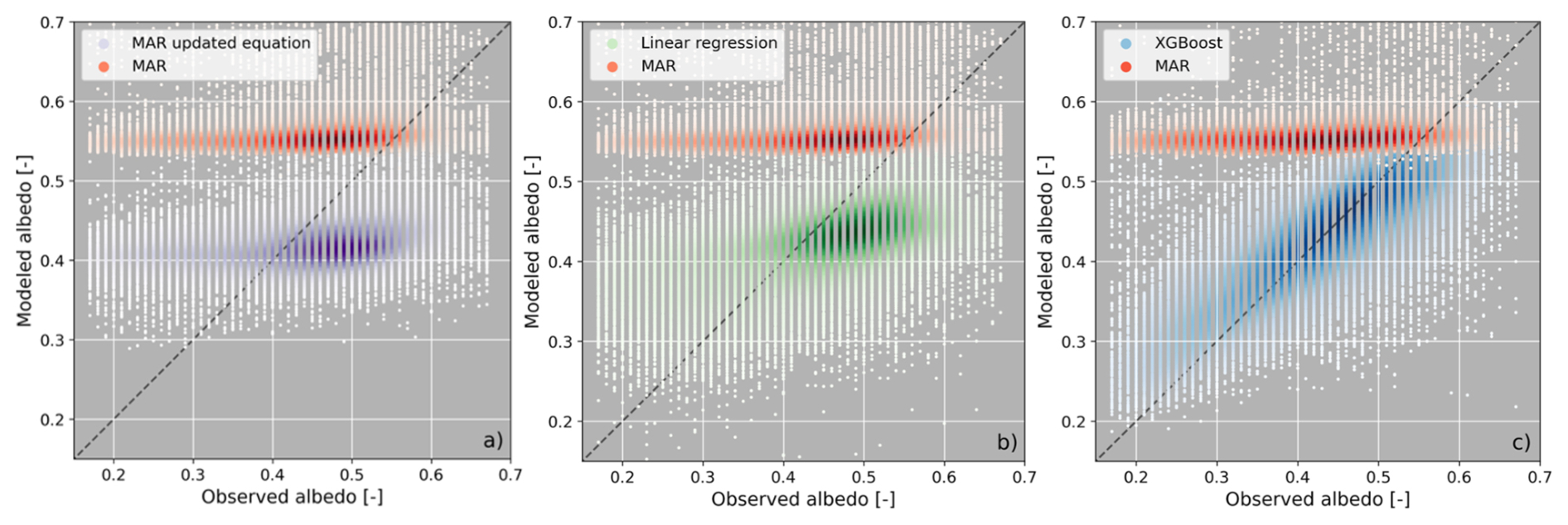
Figure 1 Scatter plot for JJA in 2020–2021 between MODIS-derived ice albedo (x axis) and ice albedo modeled with MAR (a–c; red) and ice albedo modeled with (a) the updated slope and intercept coefficients of the MAR ice albedo equation (Eq. 1) (purple), (b) linear regression with additional features (green), (c) and XGBoost (blue). The dashed line represents the 1:1 line.

4 Results

MAR tends to have low performance in predicting ice albedo when evaluated against MODIS (Fig. 1; reds) with a low coefficient of determination (R²=0.062), mean squared error (MSE = 0.032), mean absolute percentage error (MAPE = 46.202 %), and structural similarity index measure (SSIM = 0.112). The MAR albedo shows little variability with a mean of 0.56±0.04, an overestimation compared to the MODIS-derived ice albedo observations, which have a mean of 0.42±0.11.

4.1 Linear regression

The two baseline linear regression approaches, described in Sect. 3.1, show an improvement over the ice albedo modeled with MAR, with slightly better performance metrics when evaluated against the MODIS-derived ice albedo. The improved slope (0.35) and intercept (0.20) compared to the MAR ice albedo equation (Eq. 1 and Sect. 2.1) result in a factor 2–3 improvement of the R²=0.092, MSE = 0.009 and MAPE = 22.385 % (Fig. 1a; purples). However, a slight reduction is seen for the SSIM = 0.103. While the updated MAR equation provides a mean ice albedo of 0.42±0.03, similar to the mean MODIS-derived ice albedo, it shows insufficient variability and generally underestimates the MODIS-observed ice albedo.

The ice albedo derived from the linear regression with runoff, surface slope, and the additional features mentioned in Sect. 3.1 shows a moderate improvement on the test set with regard to MAR, with R²=0.202, MSE = 0.008, MAPE = 20.309 %, and SSIM = 0.285 (Fig. 1b; greens). Adding additional features beyond the seven most important ones did not achieve better performance. The additional features we tested are: meltwater production (ME, mmWE d⁻¹), longwave downward radiation (LWD, W m⁻²), surface atmospheric pressure (SP, hPa), ice density (RO1, kg m⁻³), liquid water content (WA1, kg kg⁻¹), snowfall (SF, mmWE d⁻¹), and rainfall (RF, mmWE d⁻¹). The linear regression-derived ice albedo has a mean of 0.42±0.05 but still generally underestimates the MODIS-derived ice albedo. The spread in the linear regression-derived albedo values is larger than for MAR and the updated MAR equation. However, the large variability seen in the MODIS-derived ice albedo is not achieved with the linear regression.

4.2 XGBoost

The ice albedo modeled with XGBoost shows major improvements on the test set in all performance metrics with R²=0.568, MSE = 0.005, MAPE = 14.646 %, and SSIM = 0.624. The XGBoost-modeled ice albedo has a mean of 0.42±0.08, and exhibits a variability similar to the MODIS-derived ice albedo. XGBoost represents ice albedo values between 0.4 and 0.6 well but slightly overestimates low-albedo values (Fig. 1c; blues).

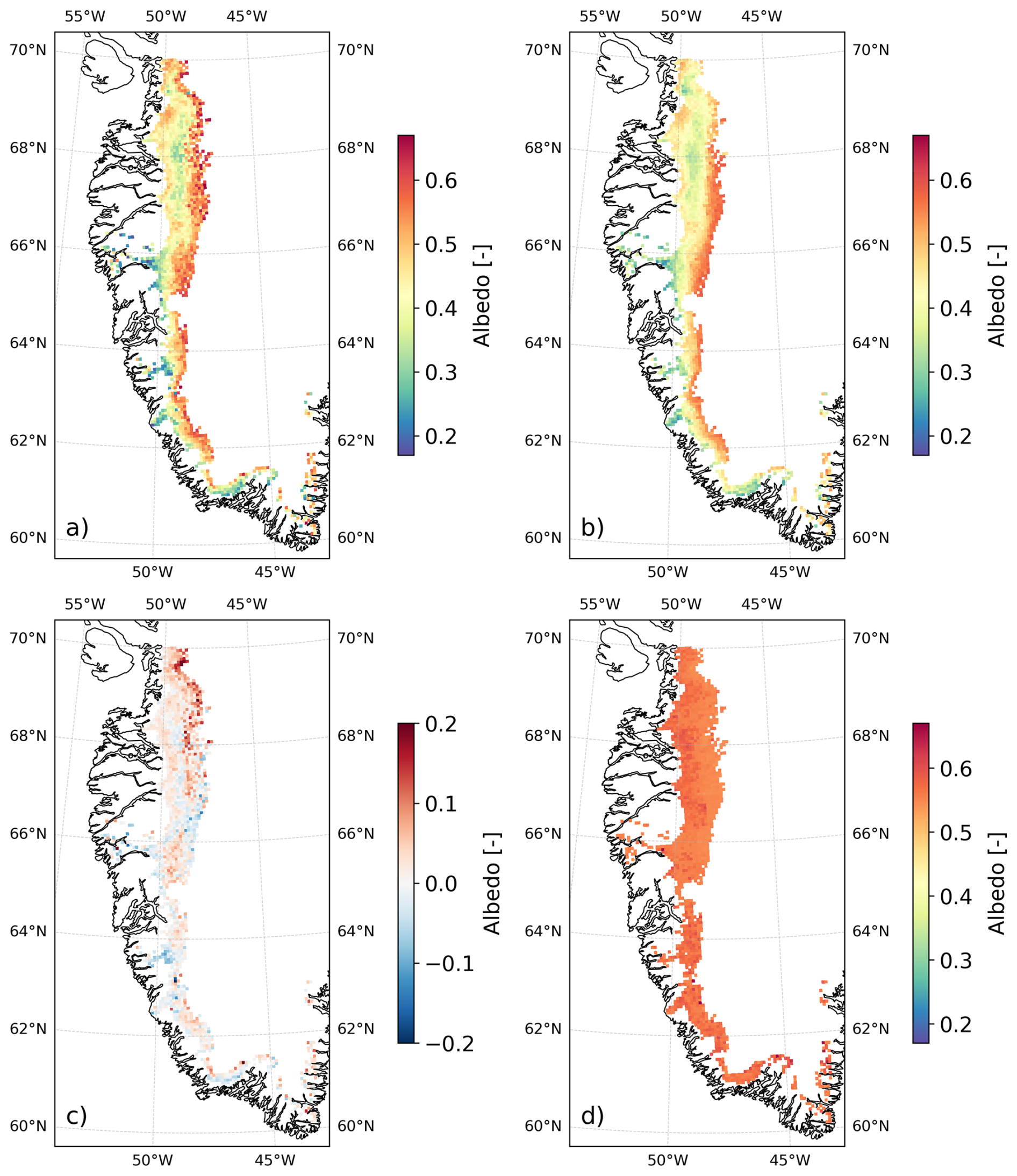
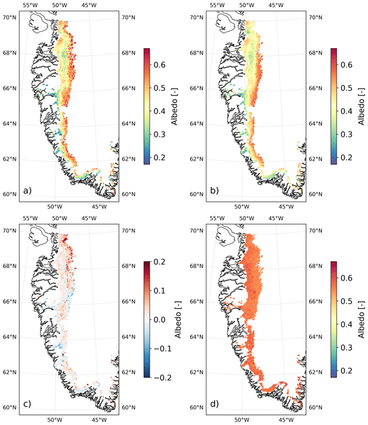
Figure 2 Mean ice albedo for JJA in 2020–2021 for (a) MODIS, (b) XGBoost, (c) difference MODIS-XGBoost, and (d) MAR.

Figure 2a shows the mean MODIS-derived ice albedo for JJA in 2020–2021. The ice albedo modeled by XGBoost (Fig. 2b) below 66° N shows a similar decreasing pattern in ice albedo from the snowline to the ice sheet margin as observed with MODIS. Above 66° N, the XGBoost-modeled ice albedo exhibits a bimodal distribution, similar to MODIS, with high values near the ice margin and near the snow line. Low albedo values are found in between the margin and snow line, which represent the dark ice zone. Compared to the MODIS-derived ice albedo, the XGBoost slightly underestimates albedo at the snowline near Jakobshavn Glacier at 69–70° N and slightly overestimates albedo in some areas near the ice margin in the central and southern regions (Fig. 2c). Generally, the XGBoost provides a higher spatial ice albedo variability across the study area than MAR (Fig. 2d).

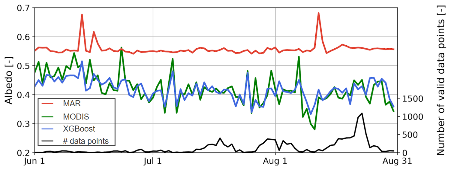
Figure 3 Daily mean ice albedo across the southwestern GrIS for JJA averaged over 2020 and 2021 (test set) for MAR (red), MODIS (green), and XGBoost (blue). The black line indicates the mean number of ice albedo data points per day.

Additionally, XGBoost provides considerable improvements in temporal ice albedo modeling compared to the ice albedo from MAR. Figure 3 shows the ice albedo during JJA averaged over 2020 and 2021. XGBoost (blue line) shows close daily alignment with the MODIS-derived ice albedos (Fig. 3: green line) throughout the melting season. Especially in July and August, when larger ice areas are exposed compared to earlier in the melting season (Fig. 3; black line) (Antwerpen et al., 2022; Noël et al., 2019). In the first half of June, when ice exposure is low, XGBoost slightly underestimates the MODIS-derived ice albedo while still outperforming MAR (Fig. 3; red line). Generally, XGBoost slightly underestimates high-albedo values and slightly overestimates low-albedo values. The peak albedo values (>0.6) from MAR represent data points with fresh snow or firn cover that have been misidentified as ice. Anomalously high albedo values can occur, especially during low ice exposure days, due to a skewed average when only a few data points are available.

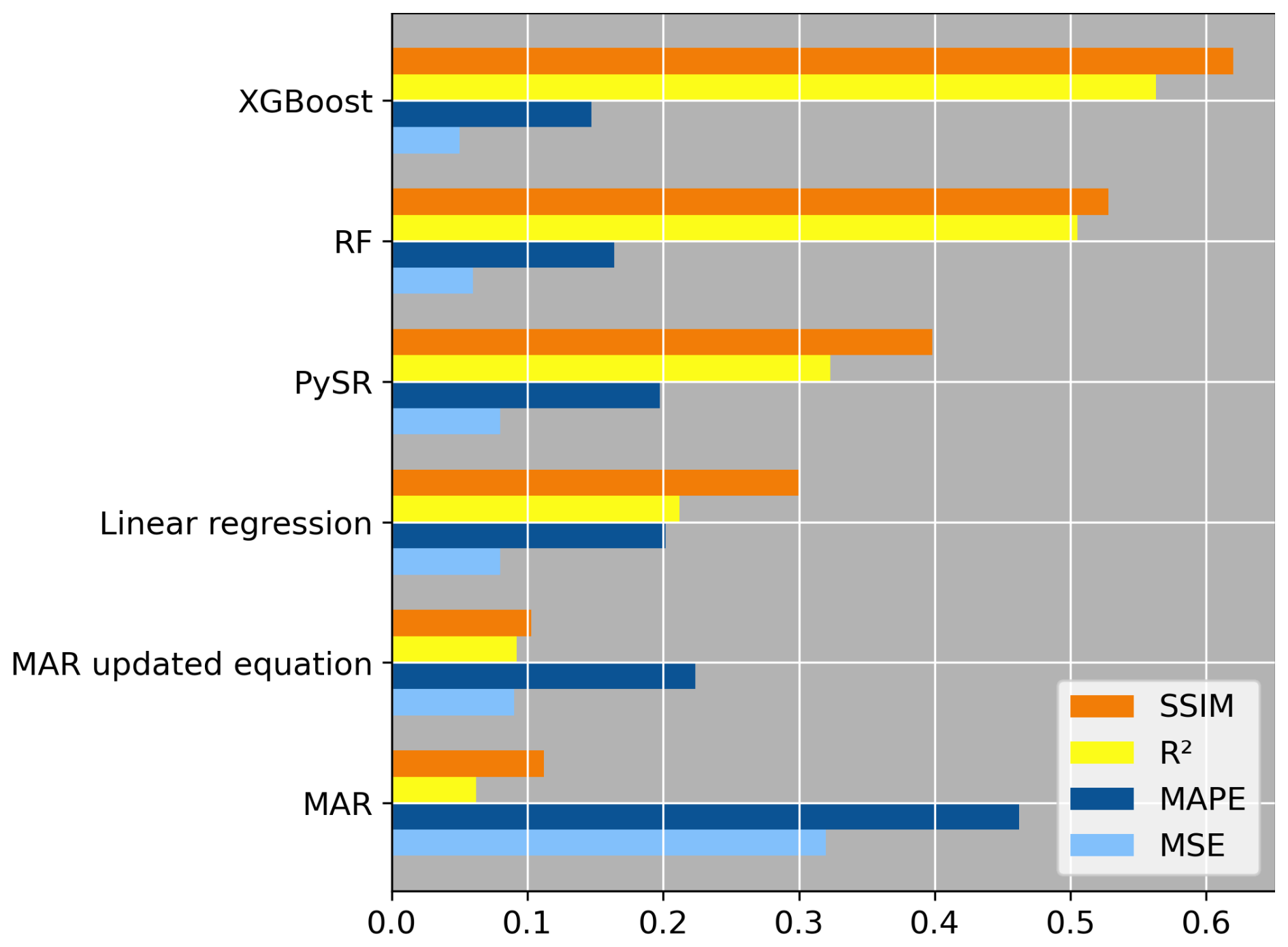
Figure 4 Performance metrics of ice albedo models vs MODIS-derived albedo. For visualization purposes, MSE is multiplied by 10 and MAPE is divided by 100. For MSE and MAPE, lower scores represent a better performance. For R² and SSIM, higher scores represent a better performance.

4.3 Model performance evaluation

The performance metrics of all our ice albedo model configurations evaluated against the MODIS-derived ice albedo observations are shown in Fig. 4. The correlations between the ice albedo modeled with RF and with PySR and the ice albedo observed with MODIS are shown in Figs. A1 and A2. The ML architectures (XGBoost, RF, and PySR) perform considerably better than the non-ML architectures (MAR, updated MAR equation, and linear regression), showcasing the superiority of ML in modeling ice albedo. While the symbolic regression method used in the PySR architecture can provide explicit insights into the developed ice albedo model, it shows a considerably lower performance than the XGBoost. We, therefore, do not use the symbolic regression insights from PySR in this study as they still have low predictive power. The RF architecture shows considerable improvement over MAR. However, the XGBoost model shows optimal performance with the highest R² and SSIM scores and the lowest MSE and MAPE scores.

4.4 SHAP analysis

Our PIXAL algorithm includes two parts: a predictive model, based on XGBoost, and an explainable AI component to reveal the drivers of ice albedo that can be used to gain insights into potential MAR model improvement. The SHAP values of the seven most important MAR-based features are listed in Fig. 5. The importance of each feature in controlling ice albedo is determined by the magnitude of its impact on the final ice albedo prediction from XGBoost (SHAP value), with respect to the mean ice albedo prediction of 0.42. In other words, a feature's SHAP value represents the extent to which that variable pushes the prediction above or below that mean. The features in Fig. 5 are ordered by the mean absolute SHAP values, which emphasizes the average impact and gives less weight to high-magnitude SHAP values. The topographic features of surface height and slope, as well as temperature, are the key drivers of ice albedo. Radiative and atmospheric features are important additional drivers. The significance and impact of each variable listed in Fig. 5 is described in more detail in Sect. 5.1.

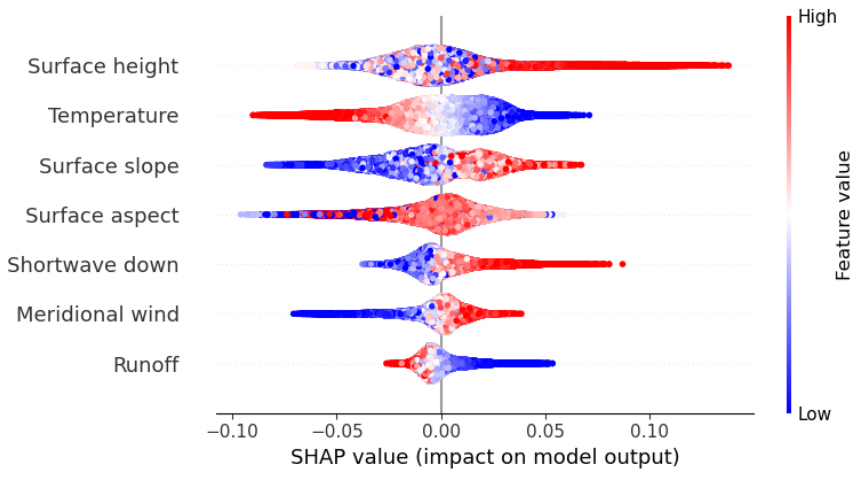
Figure 5 SHAP values for the seven most important MAR features. The SHAP value represents the impact a feature has on the ice albedo prediction, relative to the mean ice albedo prediction. A feature with a positive SHAP value indicates that the feature increases the ice albedo prediction and vice versa. The features are sorted by their mean absolute SHAP values in ascending order. Red indicates high feature values and blue indicates low feature values.

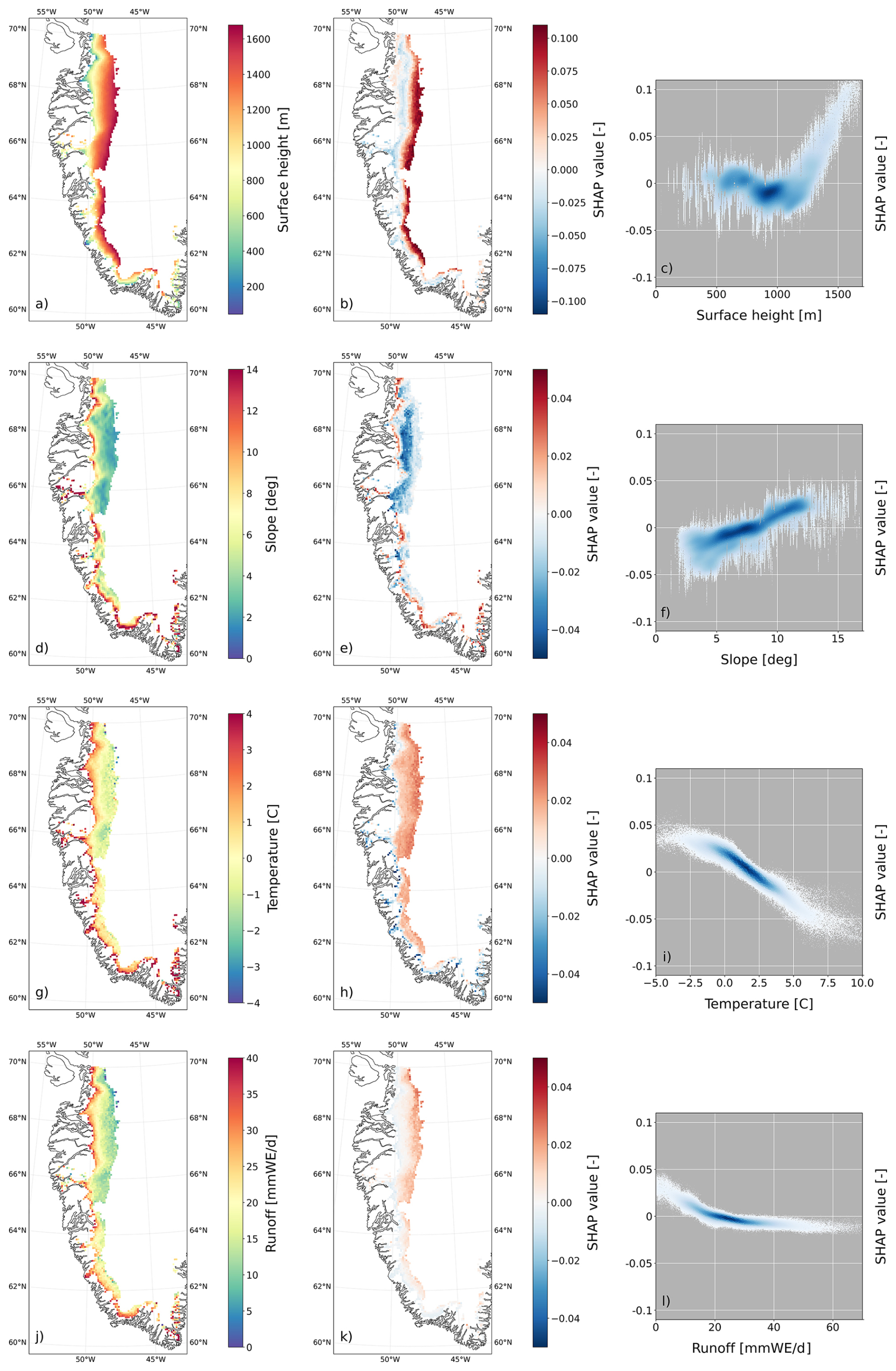
Figure 6 Feature values, SHAP values (impact of feature values on ice albedo), and the feature and SHAP value correlation for surface height (a–c), slope (d–f), near-surface air temperature (g–i), and runoff (j–l). The maps show the average over JJA in 2020–2021. Note the larger range of SHAP values for surface height in (b), compared to the SHAP value range used in (e), (h), and (k).

5 Discussion

5.1 Drivers of ice albedo

Surface height exhibits a nonlinear relationship with its SHAP values (Fig. 6a–c). The SHAP values show the strong impact of surface height on albedo, ranging from −0.05 to 0.1, with the lowest albedo values present at low elevations near the ice margin and high albedo values present at high elevations near the snow line. These findings are in line with previous studies on ice albedo drivers (Feng et al., 2024; Moustafa et al., 2015). As the melting season commences and temperatures rise, snowmelt first occurs at the ice margin, exposing the underlying ice. The snowline then retreats to higher elevations, resulting in lower-elevation ice experiencing longer exposure. Longer ice exposure can result in a lower albedo as it allows for more accumulation of LACs from local and distant sources. Algal blooms are also given more time to grow and spread if uninterrupted by snowfall events. Snowmelt events at higher elevations may add to the LAC concentrations at lower elevations when meltwater is transported toward the ice margin and LACs may remain behind on the ice surface. Higher ice sheet elevations are generally further from local LAC sources, such as moraines, dunes, dry proglacial floodplains, ground transport, and industry, reducing the potential for LAC deposition. Furthermore, englacial Holocene dust mostly melts out at lower elevations due to the flow configuration of the GrIS, adding to the LAC concentration and albedo darkening at low elevations (MacGregor et al., 2020; Wientjes et al., 2012). A large low-albedo region is present at ∼800–1100 m a.s.l. above 66° N, representing the dark ice zone where the highest concentrations of LACs are found (Shimada et al., 2016; Wang et al., 2020). Moreover, at low elevations, older, denser ice is exposed, which has fewer and smaller englacial air bubbles, reducing the albedo.

Conversely, longer ice exposure can cause an increase in albedo. Ice erodes as it is exposed to the environment in strong incoming shortwave radiation conditions, affecting the metamorphic state and creating a porous weathering crust with a low density (Munro, 1990). During conditions with low amounts of meltwater, a weathering crust has many interfaces between the ice and air, allowing for light scattering with a high angle, which increases albedo (Jonsell et al., 2003). The relationship between albedo and surface height will likely change in the future with increasing temperatures, expanding the melting season and causing earlier ice exposure, as well as later snow-covering. Therefore, ice is exposed for longer periods, potentially exacerbating the processes related to ice metamorphism and LAC accumulation, lowering the albedo. These processes will also occur more frequently and for longer periods at higher elevations as the snowline rises with increasing temperature. The impact of these effects on the performance of PIXAL is further discussed in Sect. 5.2.

The surface slope and its SHAP values have a linear and positive relationship, with SHAP values ranging between −0.05 and 0.05 (Fig. 6d–f). A flat ice surface, typically found at higher elevations and the dark ice zone, correlates to low albedo values. Higher albedo values are found on steeper ice surface slopes at the ice margin. This relationship likely represents the potential for meltwater and LACs to accumulate more efficiently on flat ice surfaces (Wientjes and Oerlemans, 2010; Zuo and Oerlemans, 1996). The positive relationship between surface slope and albedo is at odds with the results from Feng et al. (2024), who find that darker ice is found on steeper ice slopes. However, this relationship mostly holds for the southeastern GrIS while the link between slope and albedo is less strong for the southwestern GrIS. Note that the MODIS-derived albedo may be affected by high solar zenith angles (SZA) >55° (Wang and Zender, 2010; Alexander et al., 2014). This may introduce a negative albedo bias, especially in areas with a high ice surface slope.

While surface aspect is shown as an important driver of ice albedo in Fig. 5, this is due to the large impact of a few extreme feature values on ice albedo (Fig. A3). The common west-facing aspect angle (250–300°) does not affect ice albedo much on the southwestern GrIS (Fig. A3c). Some of the southwest-facing ice surfaces (300–360°) show a lower albedo, potentially due to increased algal bloom activity in response to increased solar radiation. However, we find no significant relationship between shortwave downward radiation and ice albedo or aspect (Fig. A4). Additionally, the 6.5 km resolution is likely not sufficient to represent the spatial variability of the aspect and its effects on ice albedo.

The topographic features in MAR do not change with time. Potential changes in the relationships between topographic features and ice albedo may, therefore, not be fully captured by MAR. Nonetheless, during the early Holocene (∼12–7 ka), the most recent period with warmer-than-present temperatures in Greenland (Badgeley et al., 2020), maximum ice margin retreat rates of the southwestern GrIS were ∼35 m yr⁻¹ (Briner et al., 2020). Assuming similar present-day retreat rates, the estimate of ice margin retreat at the end of this century would be ∼2660 m, which only constitutes ∼40 % of one 6.5 km grid cell in MAR. We, therefore, assume that the physical configuration of the GrIS will not change significantly by 2100 and that the static topographic features in MAR are sufficiently accurate for the purposes of this study.

There is a strong negative linear relationship (−0.009 °C⁻¹; R²=0.884) between near-surface air temperature and its SHAP values (Fig. 6g–i). High temperatures are generally found at the ice sheet margin, while low temperatures are found at higher elevations. Temperatures below 0 °C can cause refreezing of meltwater in the shallow subsurface ice layers and superficial meltwater ponds and streams, increasing the albedo. Conversely, temperatures above 0 °C can cause thin, freshly fallen snow layers to melt and expose the lower-albedo ice underneath. High temperatures generally promote biological growth of algal blooms (Uetake et al., 2010), decreasing the albedo. Moreover, high temperatures are mostly found near the ice margin, where there is closer proximity to local LAC sources and, thus, a higher likelihood of LAC deposition, including bioavailable nutrients, which further promotes algae growth.

Runoff has a strong negative near-linear relationship with ice albedo, for SHAP values for runoff below ∼25 mmWE d⁻¹, which can be partly explained by the dependence of runoff on near-surface temperature. In this range, runoff promotes ice albedo decrease through the accumulation of meltwater in ponds and streams and by filling up shallow microcavities in the upper ice layers. Runoff and decreasing ice albedo are further enhanced by the positive meltwater-albedo feedback. At runoff values of ∼25 mmWE d⁻¹, maximum albedo reduction is achieved and almost no further ice albedo decrease is observed (Fig. 6l). The cutoff of 25 mmWE d⁻¹ may signify a saturated ice surface and sub-surface where no more meltwater can be retained, causing any additional meltwater to run off to lower elevations. Moreover, increased runoff and meltwater production on the upper ice layers can cause increased melt-out of englacial Holocene dust and the development of cryoconite holes, further lowering the albedo.

The additional features listed in Fig. 5 are shown as important features because they are ordered by their absolute mean SHAP values, which gives more weight to the average impact of the feature and de-emphasizes high-impact SHAP values. However, these features do not show a high impact on ice albedo and are, therefore, not discussed here.

5.2 Limitations

Some MAR features can be biased due to potential dependencies on the inaccurately modeled ice albedo in MAR. This bias could be propagated to the PIXAL output. A solution to reduce this bias would be an iterative approach of embedding PIXAL in MAR, rerunning MAR, and updating PIXAL with the updated MAR output. This process can be repeated until a desired accuracy and error reduction is achieved. While this iterate-update approach is likely required before permanent embedding of PIXAL in MAR or other models can be considered, this is unfortunately outside of the scope of this study. We therefore cannot confidently comment on the impact of this approach, nor on the number of iterations required to reach a desired accuracy. We look forward to applying this method in a future publication.

Our results reveal relationships between ice albedo and environmental ice sheet conditions. Several of these drivers may account for some processes related to LAC-driven ice sheet darkening. However, PIXAL is trained on the available topographic, atmospheric, radiative, and glaciologic features in MAR and can, thus, only learn physical processes that can be inferred from these features. Additionally, other physical processes may not be fully captured by PIXAL, including the biological activity of algae, deposition of black carbon, dust, and ash released by deserts, local dried-up flood plains, forest fires, volcanic eruptions, anthropogenic emissions, and the melt-out of englacial Holocene dust. Positive feedback systems related to LACs, which could accelerate ice albedo darkening, may, therefore, also be missed. Some datasets are available that could represent these LAC-driven darkening processes, e.g. annual algal bloom data (Wang et al., 2020). However, this data is currently not available with the same spatiotemporal range and resolution as the MAR and MODIS datasets used in this study. Initial experiments showed that this 2-year annual algal bloom dataset created uneven input data availability resulting in biases and unwanted artefacts in the XGBoost output. We therefore omitted this data from our input data collection. We are unaware of other, more comprehensive datasets that are able to add sufficient information to improve the performance of the XGBoost model. Beyond adding direct observational inputs, alternative approaches to representing LAC-driven darkening processes could include proxy variables that co-vary with LAC concentration, or explicitly accounting for the contribution of unknown processes through uncertainty quantification. However, identifying reliable proxies at the required spatiotemporal resolution is an open challenge. We consider both directions valuable for future development of PIXAL.

Moreover, we use modeled estimates of the environmental features which poses limitations to the trustworthiness of the derived results. While MAR is a state-of-the-art regional climate model that has been validated over the GrIS (Fettweis et al., 2017), it still exhibits some biases, especially on albedo. Similarly, while MODIS has outstanding capabilities in measuring albedo, it has limitations related to atmospheric corrections, a fundamental reflectance data processing step. To account for radiance, reflectance, and transmittance effects due to atmospheric aerosol loading, a radiative transfer model is applied (Vermote et al., 2002). However, a per-pixel analysis of MODIS observations is infeasible due to computational costs (Vermote et al., 1997). Therefore, a simplified approach is applied using a look-up table for different aerosol loadings and sun-view geometries, potentially leading to inaccurate corrections. Further, NASA's Terra 10:30 a.m. local overpass time could incur a bias towards higher albedo measurements because the darkening effect of meltwater production will occur mostly in strong incoming radiation and high-temperature conditions during the afternoon. Moreover, some spatial variability is present in the performance of XGBoost compared to MODIS (Fig. 2c). This discrepancy may be partly due to spatial variability in the number of valid MODIS data points, which can lead to a bias in the mean observed ice albedo in areas with fewer valid data points (Fig. 2a). Lastly, MODIS exhibits a positive albedo bias above 70° N due to sun and satellite viewing angles at high latitudes (Alexander et al., 2014). The largest differences between XGBoost and MODIS albedo are found near this latitude, potentially explaining the XGBoost-MODIS discrepancy as a positive bias from MODIS rather than an underestimate from XGBoost.The relationships we find between the MAR features and the MODIS-derived ice albedo might, therefore, in part arise from model imperfections and measurement biases.

While we train PIXAL only on the southwestern GrIS ice albedo, many physical processes are generalizable and hold in other glaciated areas, e.g., the relationship between temperature, ice melting, and ice albedo change. However, some processes may be specific to the southwestern GrIS, such as the dependency of ice albedo on surface height, slope, and aspect. Moreover, processes relating to LAC deposition are likely specific to the southwestern GrIS as these are dependent on the LAC source location, atmospheric circulation patterns for transport, and topographical characteristics of the ice.

PIXAL is intended for both hindcasting and forecasting purposes. Because of the unknown effects of climate change on the environmental conditions on and near Greenland, a changing distribution of environmental feature values is expected for the rest of the century, e.g. more frequent high temperatures. Out-of-distribution values for input features generally pose a problem for the stability of tree-based models. However, the current spread of values in our large dataset (∼6σ) accounts for most of the expected extreme values. While these extreme values may become more common toward the end of the century, PIXAL is trained on and familiar with these values. We, therefore, do not expect significant issues relating to out-of-distribution values in forecasts. Except for surface height, with ice exposure likely occurring at higher and unprecedented elevations with continued atmospheric warming during the rest of the century.

Beyond these distributional considerations, we make two architectural trade-offs by opting for XGBoost as the basis of PIXAL. First, neural networks can in principle generalize outside of the training distribution, whereas tree-based models will assign out-of-distribution inputs the same prediction that is associated with the nearest boundary of the training data, effectively limiting extrapolation. However, as described above, the ∼6σ spread of our training dataset partially mitigates this limitation. Moreover, preliminary experiments showed a lower performance for NNs than tree-based approaches in modeling ice albedo. Second, tree-based models treat each grid cell as an independent data point and do not encode spatial relationships between neighboring pixels. This may limit their ability to capture spatial gradients such as those in the dark ice zone. Convolutional neural networks (CNNs) are theoretically better suited to leverage the information surrounding each pixel due to the spatially-aware nature of their convolutional kernels. However, our preliminary tests showed a superior performance of tree-based models over a CNN and a CNN-long short-term memory (CNN-LSTM) model in modeling ice albedo. Lastly, while SHAP can be applied to NNs and CNNs, these implementations rely on approximations of the SHAP values, whereas the SHAP implementation for tree-based models computes the exact SHAP values. Given the importance of model explainability to identify drivers of ice albedo variability, we opted for XGBoost as the basis for PIXAL.

6 Conclusions

We explored a suite of linear and nonlinear regression architectures to develop PIXAL and improve ice albedo estimates on the southwestern Greenland ice sheet. Our findings highlight XGBoost as the best-performing architecture, which outperforms a state-of-the-art regional climate model, MAR, in modeling ice albedo. The performance metrics as evaluated against the MODIS-derived ice albedo observations improved substantially compared to MAR with an increased R² from 0.062 to 0.563, an increased SSIM from 0.112 to 0.620, a decreased MSE from 0.032 to 0.005, and a decreased MAPE from 46.202 % to 14.699 %. We find that the most important drivers of ice albedo are the topographic features, specifically the ice sheet surface height and slope, and near-surface air temperature. Surface height has a nonlinear impact on albedo, but low albedo values are generally found at lower elevations, likely due to the longer ice exposure which induces increased accumulation of LACs, melting out of englacial Holocene dust, and algal bloom activity. The ice at lower elevations is generally older and denser and has fewer and smaller englacial air bubbles, further reducing the albedo. We find low ice albedo values on flat ice surfaces where meltwater and LACs are more likely to accumulate. A steep ice surface less efficiently retains meltwater and LACs and, therefore, has a higher potential for increased albedo. Temperatures below 0 °C can increase ice albedo by refreezing meltwater, while temperatures above 0 °C can decrease ice albedo by melting thin snow layers and promoting algal bloom activity. Additionally, we find that runoff is an important additional driver. Runoff can cause a decrease in ice albedo up to runoff values of ∼25 mmWE d⁻¹. Above this threshold, the upper ice layers are likely saturated with meltwater and the albedo does not decrease further. An explicit understanding of the emission, transport, and deposition of LACs onto the GrIS and other glaciated areas is essential for further improvements to PIXAL and general ice albedo modeling. PIXAL paves the way for a new generation of climate models that are more adept at modeling ice albedo and ice sheet melting. This work provides a significant step forward in ice sheet modeling for Earth system models and provides new insights on ice albedo and its drivers, the short and long-term future of the GrIS, and global and local sea level change.

Appendix A

A1 Model parameters for Random Forest

We perform a hyper-parameter search and find the Random Forest configuration with the best performance using a mean squared error loss function and bootstrap sampling. The configuration includes number of trees in the forest (75), minimum number of samples needed to split a node (15), minimum number of samples needed at each leaf node (8), method to determine the number of considered features for the best split (square root of number of features), maximum tree depth (25).

A2 Model parameters for PySR

The PySR architecture uses a Random Forest model for feature selection to build the symbolic expression. We set the maximum number of features to seven, which yields the following set: near-surface temperature, runoff, shortwave downward radiation, meridional wind, surface height, surface slope, surface aspect. We choose a range of potential operators $O_n^{(x,y)}$ with varying complexity n applied to (xy)∈ R²:

$$\begin{array}{c}{\displaystyle }{O}_{\mathrm{3}}^{(x,y)}=[x+yx-y,-xx\cdot y{x}^{\mathrm{2}}]\\ {\displaystyle }{O}_{\mathrm{6}}^{(x,y)}=[x/y,\mathrm{|}x\mathrm{|},\sqrt{x}{x}^{\mathrm{3}}]\\ {\displaystyle }\begin{array}{rl}{O}_{\mathrm{9}}^{(x,y)}& =\left[e^x\ln \right(x),{\log }_{\mathrm{2}}(x),{\log }_{\mathrm{10}}(x),\sin (x),\cos (x),\\ & \tan \left(x\right),\sinh \left(x\right),\cosh \left(x\right),\tanh \left(x\right)]\end{array}\\ {\displaystyle }{O}_{\mathrm{27}}^{(x,y)}=\left[x^y\tan \right(x),a\sinh (x),a\cosh (x),a\tanh (x\left)\right]\end{array}$$

Operators with low complexity are preferred by the PySR algorithm in building the symbolic expression and we set the maximum complexity to 70. The best results are obtained when we use 10 000 random samples from the training data set (JJA in 2000–2019) and restrict the model to run for 400 iterations or 18 h, whichever occurs first. Other parameters include a population size of 400, each with 100 samples, and 400 mutations to run, per 10 samples, per iteration.

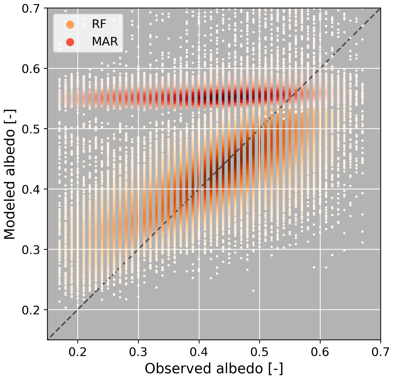
Figure A1 Correlation between MODIS-derived ice albedo (x axis) and ice albedo modeled with MAR (reds) and ice albedo modeled with Random Forest (oranges). The dashed line represents the 1:1 line.

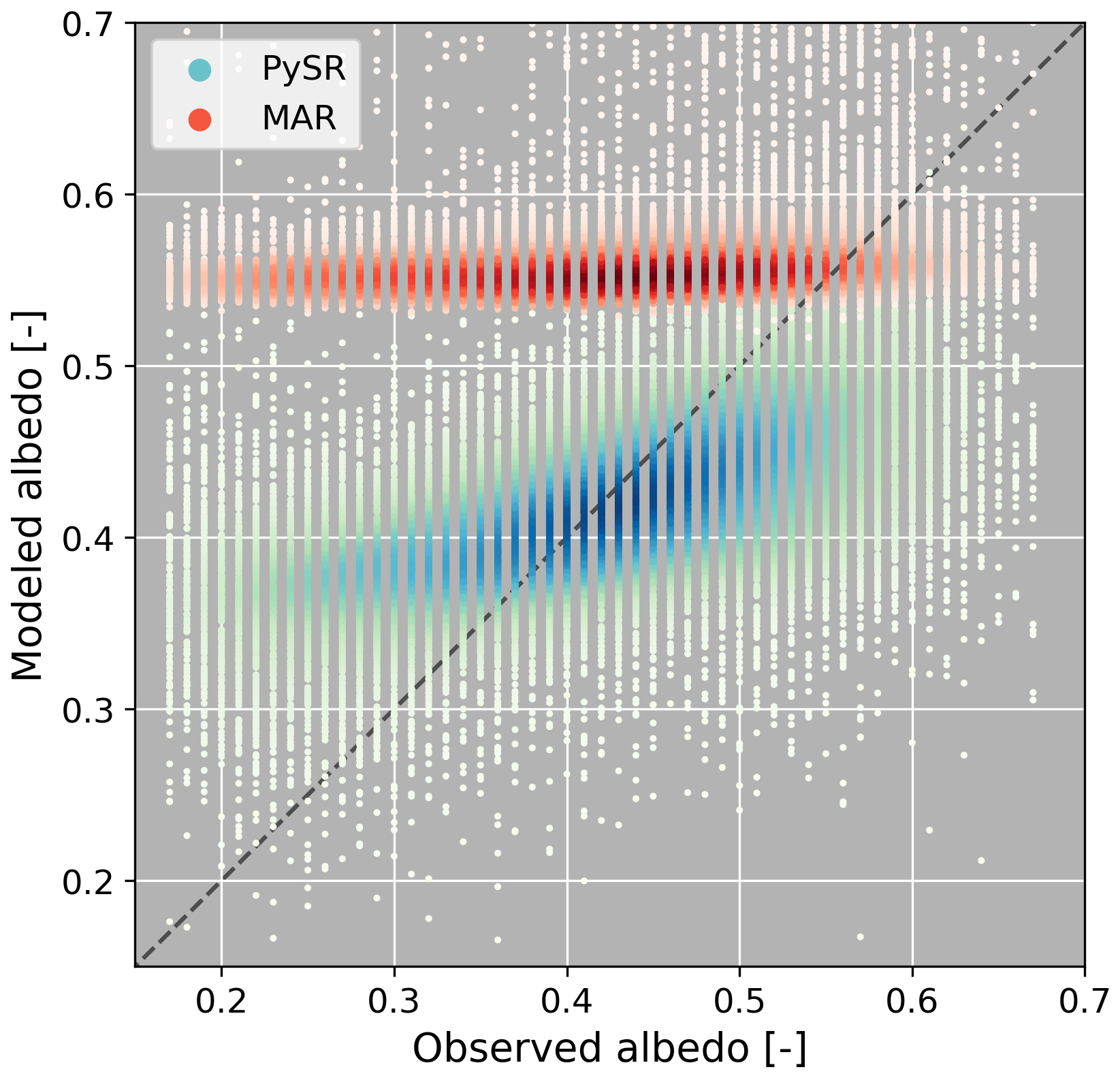
Figure A2 Correlation between MODIS-derived ice albedo (x axis) and ice albedo modeled with MAR (reds) and ice albedo modeled with PySR (green-blues). The dashed line represents the 1:1 line.

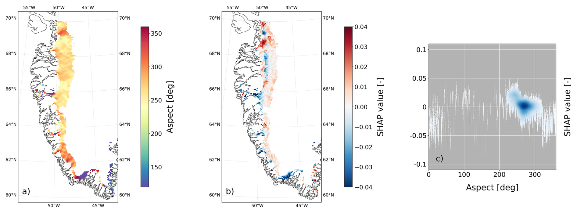
Figure A3 (a) Aspect, (b) SHAP values for aspect, and (c) their correlation. The maps show the average over JJA in 2020–2021.

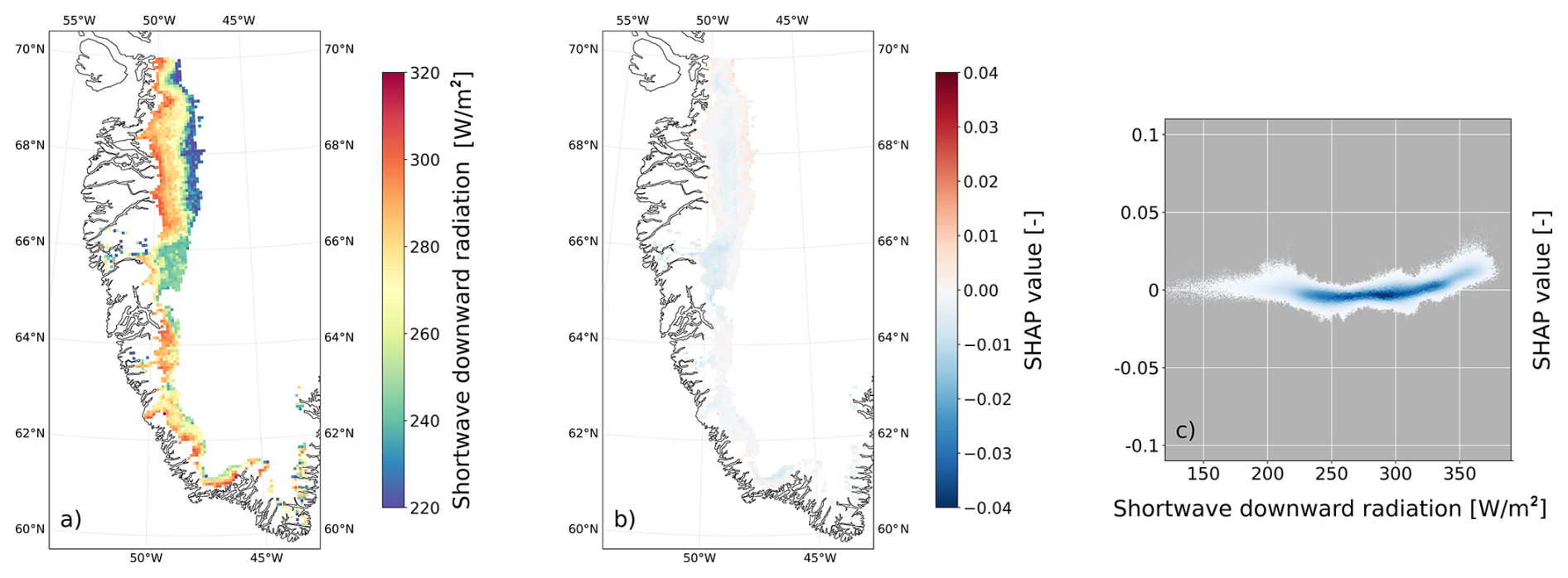
Figure A4 (a) Shortwave downward radiation, (b) SHAP values for shortwave downward radiation, and (c) their correlation. The maps show the average over JJA in 2020–2021.