Seasonal mass balance drivers for Swiss glaciers over 2010–2024 inferred from remote-sensing observations and modelling

Reliable estimates of glacier mass balance for an entire mountain range provide valuable insights into the impact of glacier melt on regional water resources. Here, we derive daily mass balance estimates for every glacier in the Swiss Alps over the period 2010–2024. To do so, we leverage two simplified surface energy-balance models and remote sensing observations, i.e. geodetic volume changes and observations of the snow-covered area fraction (SCAF) of glaciers during summer, together with machine-learning techniques for extrapolation purposes. This allows reproducing the seasonal variability of glacier mass balance for glaciers without in situ observations and determining daily glacier mass balance across Switzerland. Over the study period, the Swiss glaciers lost almost 25 % of their 2010 ice volume, which corresponds to a wastage of −15.2 ± 1.6 km³ of ice. The highest winter snow accumulation is inferred to occur in central and western Switzerland, with up to 1.5–1.9 $\mathrm{m}\mathrm{w}.\mathrm{e}.$ by the end of April, whereas the lowest winter accumulation is detected in Valais and ranges between 0.9 and 1.2 $\mathrm{m}\mathrm{w}.\mathrm{e}.$ Furthermore, winter balances are found to show better correlation in space compared to long-term annual balances, which range between −0.6 and −1.5 $\mathrm{m}\mathrm{w}.\mathrm{e}.$, indicating different dominating mechanisms. Finally, we assessed the spatio-temporal variability of seasonal mass balance to gain in-depth insights into the relation between glacier mass balance and the driving climatic factors in the Swiss Alps.

1 Introduction

Glaciers are rapidly retreating due to global warming (Hugonnet et al., 2021; The GLAMBIE Team, 2025), and monitoring the evolution of these components of the cryosphere is important to understand the driving processes involved, to assess their impact on natural hazards (Stoffel and Huggel, 2012) and water resources (Immerzeel et al., 2020), and to address the growing public interest in their changes. In the Swiss Alps, glaciers play a key role in the hydrological cycle, storing water over the winter and supplying it in the summer (Hock et al., 2005). Therefore, the availability of fresh water in Switzerland is strongly impacted by glaciers (Pellicciotti et al., 2014; Radić and Hock, 2014; Schaefli et al., 2019), but the water supplied by glaciers is expected to decrease in the future due to climate change and shrinking glaciers (Salzmann et al., 2012; Farinotti et al., 2016; Huss and Hock, 2018; Dumont et al., 2025). This leads to increasing interest in accurate monitoring of glacier mass balance and runoff on the regional scale (Anghileri et al., 2018; Patro et al., 2018; Dussaillant et al., 2025).

A widely used technique for evaluating regional mass balances is the geodetic method, which relies on differencing Digital Elevation Models (DEMs) to derive changes in the elevation of the glacier surface and thus derive changes in ice volume (Dussaillant et al., 2018; Denzinger et al., 2021; Hugonnet et al., 2021; Piermattei et al., 2024; The GLAMBIE Team, 2025). The use of this technique over short periods is linked to several challenges due to snow and firn densification processes (Huss, 2013), although recent studies proved the application potential over short periods relying on very high-resolution images (Klug et al., 2018; Vincent et al., 2021; Zeller et al., 2022; Beraud et al., 2023). Geodetic mass balance calculations are, however, still mostly performed over longer time spans, i.e. usually more than 5 years, allowing for the limitation of uncertainties. A well-suited approach for bridging this temporal gap and, thus, deriving glacier mass balance over shorter time scales is to employ modelling approaches relying on geodetic mass balance estimates for calibration (Huss et al., 2008; Compagno et al., 2021; Rounce et al., 2023). This was done extensively in the past to reconstruct glacier mass balance time series or to model the future evolution of glaciers based on calibrated models (Hock et al., 2019; Zekollari et al., 2019; Rounce et al., 2020). Despite the proven reliability of these examples for estimating annual balances, capturing the seasonal variations of mass balance remains a significant challenge (Barandun et al., 2021; Schuster et al., 2023; Cremona et al., 2025). This is a consequence of the limited observations available to constrain models, which leads to parameter equifinality and thus to inaccurately constrained seasonal variability (Finger et al., 2011; Gabbi et al., 2014). For that reason, current estimates of the seasonal glacier mass balance at the scale of the Swiss Alps are calculated based on statistical upscaling of the seasonal variability inferred from a set of about 20 glaciers with seasonal in situ observations (GLAMOS, 2024c; van Tiel et al., 2026). However, a comprehensive quantitative analysis with high spatio-temporal resolution at the regional scale relying on glacier-specific modelling and remote sensing observations is still lacking.

Several studies suggested different strategies to incorporate remote-sensing observations at high temporal resolution, which are often available at the scale of entire regions, to better constrain glacier mass balance (Hock et al., 2007; Huss et al., 2013; Hulth et al., 2013; Barandun et al., 2018, 2021). One of the most recent approaches, presented by Cremona et al. (2025), constrains the seasonal variability of glacier mass balance by relying on observed mean mass balances and observation of the snow-covered area fraction (SCAF), derived from weekly to monthly satellite imagery, together with a glaciological model. In this study, we employ this approach to derive daily mass balance estimates for each of the 1400 glaciers in the Swiss Alps over the period 2010–2024. In contrast to Cremona et al. (2025), here we additionally account for the effect of supraglacial debris cover and changing glacier area, which is relevant for regional-scale assessments (Elsberg et al., 2001; Rounce et al., 2021). Some Swiss glaciers are strongly debris-covered and small glaciers experienced significant changes in area over the 15-year study period (Linsbauer et al., 2021). Therefore, these effects cannot be neglected.

Regional mass balance estimates are strongly dependent on the geodetic mass balance (Zemp et al., 2019; The GLAMBIE Team, 2025). The last complete assessment of geodetic mass balance covering all glaciers of the Swiss Alps spans the period 1980–2010 (Fischer et al., 2015). Note that there are additional recent regional to global-scale assessments of the geodetic change of glacier mass on the scale of the European Alps (e.g. Sommer et al., 2020; Hugonnet et al., 2021), but these datasets are not comparable in terms of spatial resolution or the baseline inventory data used. Therefore, considering the extreme changes the Swiss glaciers experienced in the last decade (Cremona et al., 2023; GLAMOS, 2024a), we calculate changes in ice volume by differentiating a large set of DEMs from different sources for the Swiss glaciers between 2006 and 2023. These ice volume changes are then combined with SCAF observations derived from Sentinel-2 (available from 2015 to 2021) to constrain model parameters during calibration. This procedure is applied to 87 mostly large glaciers with available SCAF observations, which are distributed across all regions of Switzerland. Then, the model parameters are extrapolated using machine learning to the rest of the glaciers, and the daily mass balance for every glacier in the Swiss Alps over 2010–2024 is extracted. We derive changes in ice volume for the Swiss Alps over the study period. We assess regional differences in mass balance and its daily to annual temporal variability, identifying and discussing the main climatic drivers for glacier mass balance in Switzerland. Finally, we compare our results with existing estimates from upscaling approaches, e.g. (GLAMOS, 2024c), and discuss the strengths and limitations of the individual methodologies.

2 Study Site and Data

According to the last Swiss Glacier Inventory (SGI Linsbauer et al., 2021), the Swiss Alps comprised 1400 glaciers, resulting in a total glacierized area of 961 km² in 2016 (Fig. 1). For 1344 glaciers (98 % of the total glacier area) a set of multiple DEMs is available over the study period, allowing us to derive geodetic ice volume changes (see Sect. 3.1, Fig. 2). The DEMs used in this study are derived from aerial images acquired by the Swiss Federal Office of Topography (swisstopo) over the period 2006–2023. Swisstopo acquires a first set of aerial images within the standard program covering all of Switzerland following a 3-year cycle (swisstopo, 2022). Furthermore, a second set of images is acquired annually by swisstopo within the so-called “cryospheric monitoring flights” (swisstopo, 2024), aiming at detailed monitoring of selected glaciers in the frame of the Glacier Monitoring Switzerland (GLAMOS) programme. The high-resolution (0.10–0.25 m) aerial images from both image sets are then processed following two separate pipelines to derive DEMs on glaciers. The first pipeline was developed by the Swiss National Forest Inventory (SNFI) and processes images from the standard 3-year-cycle program to deliver DEMs that were primarily designed for lowland applications (Ginzler and Hobi, 2015; Marty et al., 2025), thus partially resulting in lower quality over high-mountain regions and glaciers. Due to this, two additional processing steps are necessary for these DEMs. In the first step, each DEM is decomposed into the original DEM stripes resulting from different flight lines. These DEM stripes are then realigned, enhancing the relative orientation between adjacent flight lines. This is done with the OPALS Least Square Matching algorithm in overlapping areas (Pfeifer et al., 2014). In the second step, the resulting, now corrected DEM, is aligned to a common, Swiss-wide stable terrain DEM. The latter is chosen to be the swissAlti3D DEM of 2018. This two-step procedure allows for increasing the internal consistency of the SNFI DEMs over glaciers, thus enabling accurate ice volume change calculations. The second pipeline follows the standard processing chain of swisstopo and is based on an automated procedure relying on stereo correlation and photogrammetric methods, which sometimes includes information from stereoscopic 3D measurements and available laser measurements manually. More detailed information is provided by swisstopo (2022). This pipeline processes aerial images from both image sets mentioned above. All available DEMs (with a resolution of 0.5–2.0 m), resulting from both pipelines, are used to derive multiple estimates of the ice volume change over the study period (see Sect. 3.1).

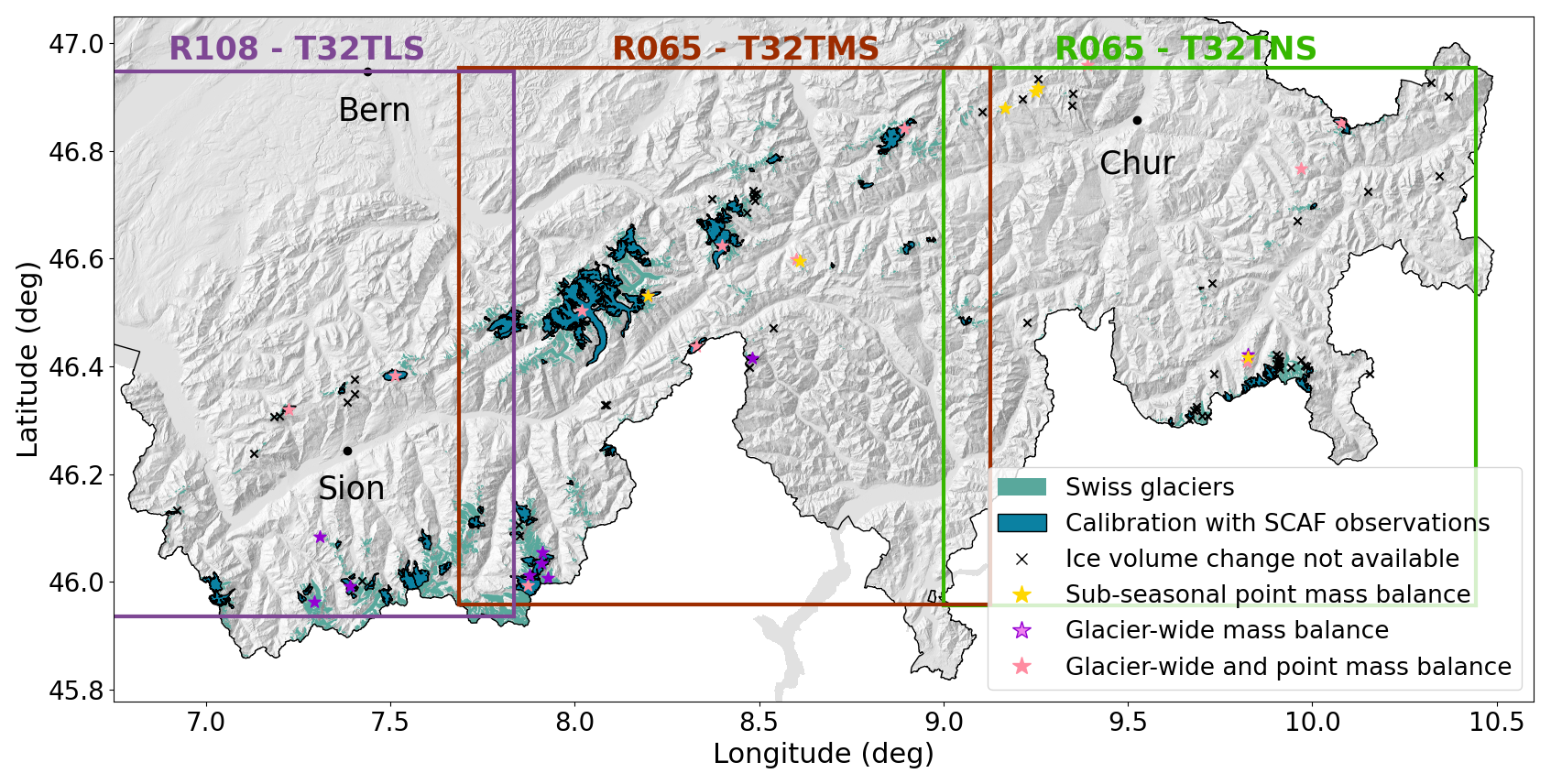
Figure 1 Overview of the study region. Glaciers are shown in teal. The 87 glaciers for which we apply the calibration with SCAF observations (see Sect. 3.2.3) are highlighted in dark teal. For the remaining glaciers, the model parameters are extrapolated relying on a machine learning approach (Sect. 3.2.4). Ice volume changes are available for 1344 glaciers. Glaciers without ice-volume change information (black crosses) and glaciers used for evaluation (coloured stars) are shown separately. For the latter, glaciers with sub-seasonal point mass balance observations (yellow stars), glaciers with seasonal glacier-wide mass balance observations (violet stars), and glaciers with both types of observations (pink stars) are distinguished. The footprints of the Sentinel-2 tiles R108-T32TLS, R065-T32TMS, and R065-T32TNS for extracting SCAF are shown in purple, red, and green, respectively.

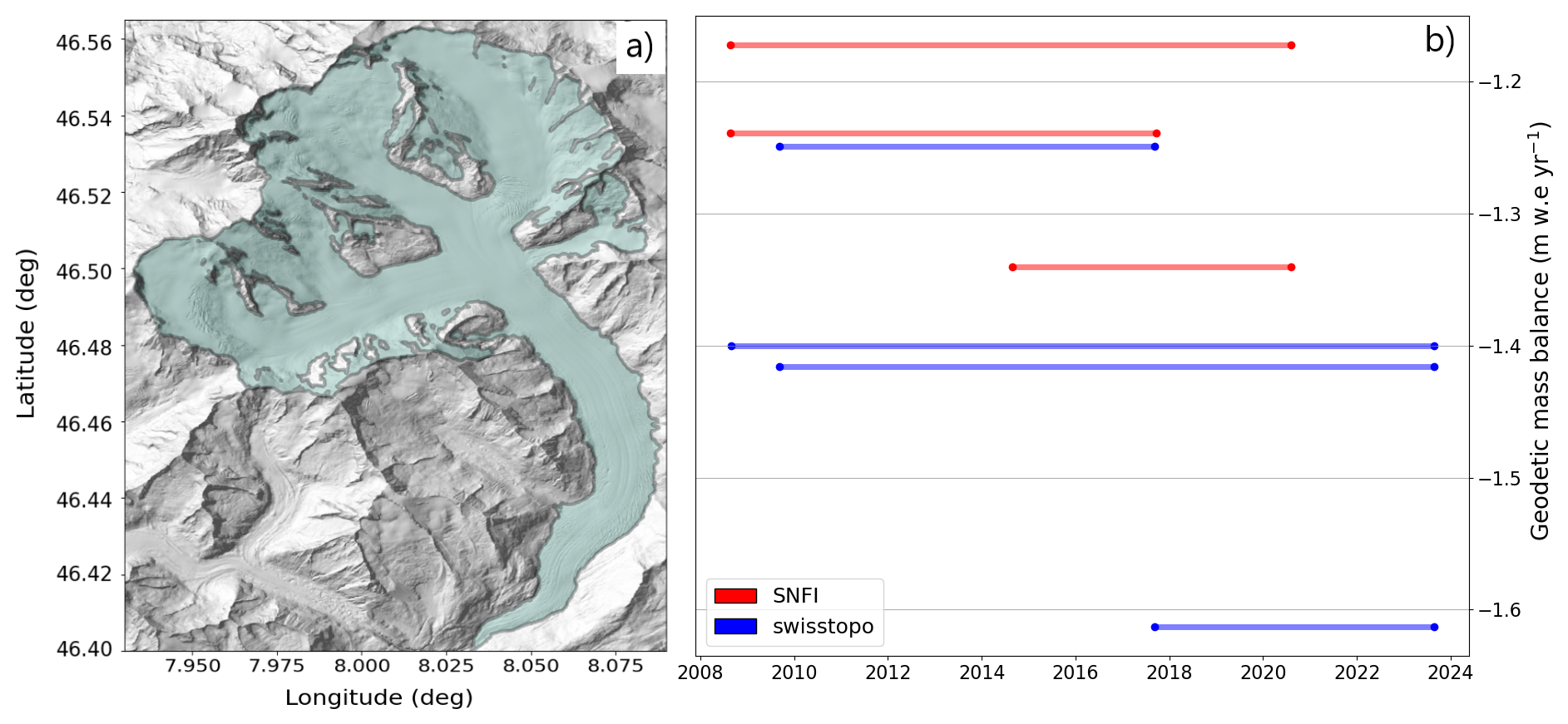
Figure 2 Temporal coverage of the geodetic ice volume changes available for Grosser Aletschgletscher. (a) Overview of Grosser Aletschgletscher with glacier outline from the SGI2016. (b) Geodetic mass balance based on the SNFI DEMs (red) and swisstopo DEMs (blue).

For 87 glaciers (highlighted in dark blue in Fig. 1), we apply a calibration relying on SCAF observations over the melt season and geodetic ice volume changes (see Sect. 3.2.3). For the remaining ∼1300 glaciers, the model parameters are extrapolated relying on a machine-learning approach and information on geodetic ice volume changes (see Sect. 3.2.4). The SCAF observations were derived by Schwaizer et al. (2023), Cremona et al. (2025) from Sentinel-2 multi-spectral L1C data during the melt seasons (June–September) over the period 2015–2021, at 10 m resolution. The derivation relied on the tiles R108-T32TLS, R065-T32TMS, and R065-T32TNS (Fig. 1), yielding an average of 21 SCAF observations per glacier in total over the period 2015–2021.

To model glacier mass balance, we force our model (cf. Sect. 3.2) with daily, gridded products provided by MeteoSwiss at a resolution of ca. 2 km. More specifically, we use daily mean temperature (T), precipitation sum (P), and daily mean incoming shortwave radiation (G) over our domain of interest (MeteoSwiss, 2018, 2021a, b).

The glacier geometry is defined using the glacier outlines provided by the SGI2016 (Linsbauer et al., 2021) and the swissALTI3D DEM (swisstopo, 2020). To account for temporal changes in glacier area, we apply a simple volume-area scaling relation, validated using area-change observations (see Sect. 3.2.2). The SGI2016 also provides information about the debris-covered area for each glacier, which is used with the sub-debris melt enhancement factors provided by Rounce et al. (2021) to account for the effect of supraglacial debris cover on mass balance (see Sect. 3.2.1).

For evaluation, the model outputs are compared against (i) seasonal glacier-specific mass balance inferred from direct measurements for 23 glaciers, included in the GLAMOS long-term monitoring programme (Huss et al., 2015; GLAMOS, 2024a), and (ii) daily to monthly point mass balance measurements available for 19 glaciers from repeated field measurements during the summer spanning periods of 7–90 d (GLAMOS, 2024b).

3 Methods

To provide daily mass balance estimates for every glacier in the Swiss Alps from 2010 to 2024, we follow the concept proposed by Cremona et al. (2025). The approach separates the accumulation and ablation components of the modelled mass balance by relying on geodetic ice volume changes and SCAF observations.

3.1 Ice volume changes

Changes in ice volume are derived using the geodetic method, which relies on differentiating DEMs of a glacier captured at different points in time to measure changes in surface elevation. The procedure for determining ice volume changes, while based on the same underlying concept for both SNFI and swisstopo DEMs, exhibits some variations to account for DEM-specific characteristics derived from the respective processing chain during DEM generation.

For the SNFI DEMs, we differentiate pairs of DEMs and derive the change in surface elevation over the glacier area by masking the glacier extent with the outlines provided by the Swiss Glacier Inventory 2016 (SGI2016, Linsbauer et al., 2021). Note that we derive ice volume changes only for pairs of DEMs that are more than 5 years apart to reduce uncertainties due to firn densification processes (Huss, 2013). After differentiating two DEMs, the difference of DEMs (DoD) is derived. However, the DoD from these DEMs contains data gaps and outliers resulting from cloud cover in the stereo images or correlation issues during DEM generation. To filter outliers, we divide the DoD into 20 m elevation bands according to a reference DEM, and for each band, we filter values that are more than one standard deviation apart from the mean elevation change of the band. The data gaps are then filled following a local hypsometric approach as implemented in the Python package xDEM (xdem contributors, 2021; Mannerfelt et al., 2022). This approach relies on the correlation between elevation and elevation change to capture the hypsometric signal of each glacier. Note that for elevation bands without any available data, an interpolation based on the elevation-dependent signal derived from the remaining elevation bands is performed (see xdem contributors, 2021 for more details). To minimise uncertainties introduced by the interpolation method, DoDs with voids exceeding 50 % of the glacier area are excluded. From the interpolated and filtered DoDs, the ice volume change is calculated by summing the values in the DoD.

Ice volume changes from the swisstopo DEMs (see GLAMOS, 2024d) were computed following a similar procedure, but with two main differences. (1) The temporally closest glacier outline to each of the two DEMs to be compared used to define glacier area and the perimeter used for evaluating surface elevation change. In addition to the SGI2016, outlines are available for most glaciers at 3- to 6-year intervals, for some glaciers even at 1-year intervals. (2) Unlike the SNFI DEMs, the swisstopo DEMs are delivered free of voids, and outliers have already been filtered during DEM generation. Therefore, the outlier filtering step and the gap filling step described above were not necessary. However, for some of these DEMs the actual acquisition dates were not traceable and only the year the DEM was known (see also Piermattei et al., 2024), thus the exact period of the corresponding ice volume change observations could not be resolved. To address this drawback, we used the consistently reported dates of the SNFI DEMs to assign the missing dates to the swisstopo DEMs, since both datasets are based on the same aerial image acquisition flights (see Sect. 2). Therefore, when only one DEM is available for a given year, the date of the SNFI DEM is also assigned to the swisstopo DEM. In years with multiple DEMs with different acquisition dates, the mean acquisition date of the SNFI DEMs for that year is taken and assigned to all swisstopo DEMs in the respective year. The standard deviation in the acquisition date indicates the temporal spread of the DEMs within that year. Ice volume changes with lower standard deviations in acquisition dates are favoured to reduce uncertainties and improve the temporal constraint on the time period of ice volume changes based on swisstopo DEMs (GLAMOS, 2024d).

As a result, for each glacier, we obtain multiple estimates of the ice volume change over the study period, which are used during model calibration. For Grosser Aletschgletscher (Fig. 2), taken here as an explanatory example, seven estimates of the ice volume change are available within the period 2006–2023, covering different years. Three of these estimates are derived from SNFI DEMs and four from swisstopo DEMs. Each of the seven geodetic ice volume changes is used during calibration in an ensemble approach, meaning that for Grosser Aletschgletscher, the ensemble consists of seven parameter sets (see Sect. 3.2.3). Across the 1400 Swiss glaciers, the number of geodetic ice volume change estimates per glacier ranges from 0–38, with an average of eight evaluated periods per glacier.

3.2 Mass balance modelling

We model the altitudinal distribution of glacier surface mass balance using CRAMPON (Cryospheric Monitoring and Prediction Online, Landmann et al., 2021), with a very similar setup as presented in Cremona et al. (2025). CRAMPON is an operational mass balance model for calculating glacier-specific mass balance on a daily scale. The model discretises a glacier into elevation bands of 20 m and for each elevation band snow accumulation and ice/snow melt is computed. Accumulation is modelled according to the concept proposed by Huss et al. (2008):

$$\begin{array}{}\text{(1)}& c_{\text{sfc}}\left(z\right)=c_{\text{prec}}\cdot P\cdot \left[\mathrm{1}+(z-z_{\text{ref}})\cdot {\displaystyle \frac{\partial P}{\partial z}}\right],\end{array}$$

where c_sfc(z) is the snow accumulation ($\mathrm{m}\mathrm{w}.\mathrm{e}.{\mathrm{d}}^{-\mathrm{1}}$) at elevation z, c_prec is the precipitation correction factor, P is the sum of solid precipitation at the reference elevation z_ref, and $\frac{\partial P}{\partial z}$ is a precipitation gradient.

To model ablation, two different melt model formulations by Hock (1999) and Pellicciotti et al. (2005) are employed. Melt in the Hock model is determined as follows:

$$\begin{array}{}\text{(2)}& a_{\text{sfc}}\left(z\right)=(\text{MF}+a_{\text{snow}/\text{ice}}\cdot I_{\text{pot}}(z\left)\right)\cdot max\left(T\right(z)-T_{\text{melt}},\mathrm{0}),\end{array}$$

where MF is the temperature melt factor ($\mathrm{m}\mathrm{w}.\mathrm{e}.{\mathrm{K}}^{-\mathrm{1}}{\mathrm{d}}^{-\mathrm{1}}$), $a_{\text{snow}/\text{ice}}$ are two radiation factors for snow and ice ($\mathrm{m}\mathrm{w}.\mathrm{e}.{\mathrm{m}}^{-\mathrm{2}}{\mathrm{d}}^{-\mathrm{1}}{\mathrm{W}}^{-\mathrm{1}}{\mathrm{K}}^{-\mathrm{1}}$), and I_pot(z) is the potential clear-sky direct solar radiation (W m⁻²). We assume T_melt=0 °C, and a ratio $a_{\text{snow}}/a_{\text{ice}}$ of 0.75 (Hock, 1999; Farinotti et al., 2012). Melt in the Pellicciotti model is determined as follows:

$$\begin{array}{}\text{(3)}& \begin{array}{rl}& a_{\text{sfc}}\left(z\right)=\\ & \left\{\begin{array}{l}\mathrm{\text{TF}}\cdot T\left(z\right)+\text{SRF}\cdot (\mathrm{1}-\mathit{\alpha }(z\left)\right)\cdot G\left(z\right)\text{if}T\left(z\right)>T_{\text{melt}}\\ \mathrm{0}\text{if}T\left(z\right)\le T_{\text{melt}},\end{array}\right.\end{array}\end{array}$$

where TF is the temperature factor ($\mathrm{m}\mathrm{w}.\mathrm{e}.{\mathrm{K}}^{-\mathrm{1}}{\mathrm{d}}^{-\mathrm{1}}$), SRF is the shortwave radiation factor (${\mathrm{m}}^{\mathrm{3}}{\mathrm{d}}^{-\mathrm{1}}{\mathrm{W}}^{-\mathrm{1}}$), α(z) is the albedo (–) parametrized following Brock et al. (2000), and G(z) is the incoming shortwave radiation (W m⁻²). Note that for this model, T_melt=1 °C (Pellicciotti et al., 2005). We then combine the outputs of the two melt models by taking the average of the computed daily melt, promoting stability in the model outputs by reducing uncertainties that may derive from the limitations of the individual melt models. The temperature at each elevation band (T(z)) in Eqs. (2) and (3) is derived as follows:

$$\begin{array}{}\text{(4)}& T\left(z\right)=T+(z-z_{\text{ref}})\cdot {\displaystyle \frac{\partial T}{\partial z}},\end{array}$$

where T is the temperature at the reference elevation z_ref of the grid cell in the meteorological product closest to the glacier centroid, and $\frac{\partial T}{\partial z}$ is the temperature lapse rate derived with linear regression from temperature values of the five surrounding cells.

To model the evolution of snow cover on top of the glacier ice, we assume an initial snow depth of zero across the entire glacier at the start of the study period. The snow water equivalent of each elevation band is subsequently updated according to the modelled climatic mass balance, i.e. the daily accumulation and melt. At each time step, the modelled snow-covered area fraction is derived by summing the area of all elevation bands with a snow depth greater than zero with respect to the beginning of each hydrological year, and dividing this total by the glacier area.

3.2.1 Debris cover

Supraglacial debris cover has a significant effect on melt enhancement or reduction for the ice underneath (Nicholson and Benn, 2012; Rounce et al., 2021). To account for this effect, the modelled melt resulting from Eqs. (2) and (3), corresponding to those of clean ice, is scaled with a sub-debris melt enhancement factor. A sub-debris melt enhancement factor below 1 indicates that the debris protects the ice, leading to reduced melt compared to clean ice. This is often the case for a thick layer of debris with a significant isolation effect on the underlying ice. Vice versa, a sub-debris melt enhancement factor above 1 indicates enhanced melt compared to clean ice, which is typical for a thin layer of debris that offers virtually no isolation effect but decreases the surface albedo. For glaciers larger than 2 km², we use the distributed sub-debris melt enhancement factor provided by Rounce et al. (2021), which is derived by relying on Landsat-8 images spanning 2013–2018 combined with modelling. At each elevation band, the average sub-debris melt enhancement factor from Rounce et al. (2021) (${\stackrel{\mathrm{‾}}{E}}_d$) is multiplied with the modelled melt from Eqs. (2) and (3) as follows:

$$\begin{array}{}\text{(5)}& a_{\text{sfc, deb}}=a_{\text{sfc}}\cdot {\stackrel{\mathrm{‾}}{E}}_d\end{array}$$

Note that this occurs only for snow-free elevation bands, i.e. bands with a modelled snow depth larger than zero (see also Sect. 3.2). For glaciers smaller than 2 km², Rounce et al. (2021) did not calculate the sub-debris melt enhancement factor. For these glaciers, we derive the sub-debris melt enhancement factor for each elevation band by using the debris-covered area provided by the SGI2016 and assuming a sub-debris melt enhancement factor of 0.63 over this area, i.e. the mean value found by Rounce et al. (2021). In this approach, the sub-debris melt enhancement factor remains constant over time for each elevation band, i.e. debris thickness and characteristics are assumed to remain unchanged over the study period, under consideration of the geometry corresponding to the year of the SGI2016.

3.2.2 Glacier area evolution

To model the evolution of the glacier area over the study period, we employ the approach proposed by Möller and Schneider (2010). The approach relies on the volume-area scaling law (Bahr et al., 1997), which relates the volume and the area of a glacier with a power law as:

$$\begin{array}{}\text{(6)}& V=c\cdot A^{\mathit{\gamma }},\end{array}$$

where V is the glacier volume, A the glacier area, γ a dimensionless scaling exponent, and c a scaling coefficient. Möller and Schneider (2010) apply the volume-area scaling law to relate changes in glacier volume and area. Following this concept, the glacier area at the end of every year is updated as follows:

$$\begin{array}{}\text{(7)}& A_{y+\mathrm{1}}={\left({\displaystyle \frac{V_y+\mathrm{\Delta }{V}_y}{c}}\right)}^{\frac{\mathrm{1}}{\mathit{\gamma }}},\end{array}$$

where V_y is glacier volume at the end of the previous year, ΔV_y is the volume change over the current year, and γ and c are the scaling exponent and coefficient as in Eq. (6). We use Eq. (7) to infer evolving glacier area with γ=1.36 according to the literature (Bahr et al., 2015), and directly calculating c with the glacier-specific area and volume known for the year of the SGI2016 (Linsbauer et al., 2021; Grab et al., 2021). Since the area and volume for the inventory date are given, this year serves as our starting point for the glacier area updating forward (up to 2024) and backwards in time (to 2010). This is achieved by first calculating the cumulative yearly mass balance with Eqs. (1)–(3), which allows deriving the ΔV_y, and subsequently calculating the glacier area with Eq. (7) for the next time step (see also van Tiel et al., 2026). To update the area-elevation distribution of our model domain, it is assumed that all changes in glacier area occur in the ablation zone, i.e. below the median glacier elevation according to the geometry of the SGI 2016. We attribute computed relative annual area changes equally to all bands below this mean equilibrium line altitude, corresponding to the center of the study period. This means that each elevation band in the lower part of the glacier shows the same annual area changes in relative terms. Since this is a considerable simplification of actual retreat dynamics, the associated limitations are discussed in Sect. 4.4.

3.2.3 Model calibration

The mass balance model is calibrated relying on the concept described in Cremona et al. (2025), i.e. by combining information from SCAF observations and geodetic ice volume changes with a three-step optimisation procedure (Fig. 3). In the first step, the parameters of the melt models (MF and $a_{\text{snow}/\text{ice}}$ in Eq. 2, and TF and SRF in Eq. 3) are adjusted to reproduce the observed geodetic ice volume change. Here, a density of volume change of 900 kg m⁻³ is assumed to convert mass change to ice volume change. This assumption is motivated by the almost complete disappearance of firn areas observed since the beginning of the 21st century in the Swiss Alps, resulting in a rapid decline in the importance of firn processes in the investigated region (Menounos et al., 2025). In the second step, the accumulation parameter, i.e. c_prec in Eq. (1), is optimised in order to minimise the difference between modelled and observed SCAFs over the melt seasons 2015–2021, i.e. the value of c_prec that provides the lowest Root Mean Square Error (RMSE) between observed and modelled SCAFs is selected (for more details refer to Cremona et al., 2025). In the third step, the temperature lapse rate is adjusted to further optimise the model's reproduction of the observed SCAF. This step is new with respect to the procedure presented in Cremona et al. (2025), and it addresses the significant impact of the temperature lapse rate on the altitudinal distribution of mass balance and, hence, on the modelled course of the SCAF during the melt season. The initial estimate of the temperature lapse rate is based on the gridded temperature data, deriving the gradient from the temperature and elevation of the cells next to the glacier. This provides insight into the lapse rate for a wider area, but neglects local patterns. We then refine this estimate by adjusting the temperature gradient in 5 % increments, selecting the value that minimises the difference between modelled and observed SCAFs.

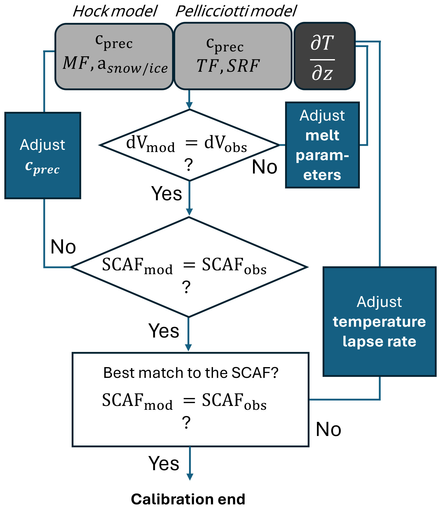
Figure 3 Three-step model calibration scheme. In the first step, the melt parameters (MF, $a_{\text{snow}/\text{ice}}$, TF, and SRF) are adjusted to match the observed ice volume change. In the second step, the precipitation correction factor (c_prec) is adjusted to optimise the reproduction of the observed SCAF over the melt seasons. In the third step, the temperature lapse rate is adjusted to further minimise differences between modelled and observed SCAF.

This procedure is applied for every value of the ice volume change available from the swisstopo DEMs (GLAMOS, 2024d) and the ones derived in this study from the SNFI DEMs, resulting in one parameter set for each value of a geodetic ice volume change inferred over various periods of at least 5 years between 2010 and 2024, whereby parameters remain constant over the study period. This calibration is applied to 87 glaciers with available SCAF observations, and across these 87 glaciers the number of parameter sets ranges from 1–20, with an average of 5 parameter sets per glacier. For each parameter set, the daily mass balance over 2010–2024 is calculated, i.e. in an ensemble approach, and the final estimate for the daily mass balance corresponds to the resulting mean of this ensemble. The ensemble spread is used to derive the uncertainty of our mass balance estimates (see Sect. 3.4). It is important to note that this calibration approach does not rely on direct field observations, which is a substantial advantage for regional-scale assessments.

3.2.4 Extrapolation of the precipitation correction factor

A comprehensive quantitative assessment of regional mass balance requires reliable estimates of model parameters for all glaciers in the region. Therefore, the parameters derived for the 87 glaciers must be extrapolated to the remaining Swiss glaciers that lack SCAF observations. This extrapolation is done using machine learning, which is widely applied across earth sciences (Zhang et al., 2022), including several examples in glaciology (Bolibar et al., 2020; de Roda Husman et al., 2024; van der Meer et al., 2025), to capture spatio-temporal relations of environmental variables. In this study, we use eXtreme Gradient Boosting (XGBoost, Chen and Guestrin, 2016), a supervised-learning model consisting of an ensemble of decision trees that are built sequentially during training, and we aim to extrapolate the accumulation parameter c_prec across all Swiss glaciers. The attributes used for the extrapolation are the geographic coordinates, i.e. the longitude and latitude of the glacier centroid, the median glacier elevation, the median glacier slope, the median glacier aspect, and the glacier area. These attributes are given in the SGI2016. We also tested including additional predictors, namely the average mean summer temperature, the average total winter precipitation, and the average temperature range, which are related to the climatological conditions of each glacier and could thus potentially improve model performance. However, since these variables did not lead to a significant improvement of the results, we chose not to include them in order to maintain a parsimonious set of predictors for the machine-learning approach.

The hyperparameter space of the XGBoost model is constrained by the maximum tree depth $\in [\mathrm{2},\mathrm{8}]$, the number of estimators $\in [\mathrm{10},\mathrm{700}]$, and the learning rate $\in [\mathrm{0.01},\mathrm{0.3}]$. To identify the best model, a randomised grid search with five-fold cross-validation over the hyperparameter space was performed. In each fold, approximately 70 glaciers are used for training and about 20 glaciers for testing. This results in a model that reproduces c_prec with a mean cross-validation RMSE over the five folds of 0.37 (–) and a mean absolute percentage error (MAPE) of 13 %. The model performance to predict seasonal and annual mass balance for glaciers relying on extrapolated c_prec is evaluated in Sect. 3.3. This model is employed to extrapolate the precipitation correction factor c_prec to approximately 1300 glaciers. The resulting c_prec values range from 1.1 to 3.5, with a Swiss-wide area-weighted average of 1.8. Afterwards, for each glacier, the melt parameters are tuned to match the ice volume changes. As before, because there are multiple ice volume changes available for every glacier (see Sect. 3.1), multiple parameter sets are available for every glacier. For each of these parameter sets, the daily mass balance is calculated, i.e. in an ensemble approach, whereby the size of the ensemble depends on the number of geodetic estimates used during calibration. The extrapolation enables us to provide daily mass balance estimates over 2010–2024 for 1344 glaciers (98 % of the glacier area). For the remaining glaciers, for which no change in ice volume is available, the mass balance is assumed to be equivalent to the average daily Swiss-wide mass balance. Across Swiss glaciers, MF ranges from 0 to 9 $\mathrm{m}\mathrm{w}.\mathrm{e}.{\mathrm{K}}^{-\mathrm{1}}{\mathrm{d}}^{-\mathrm{1}}$, with a median of 1.79 $\mathrm{m}\mathrm{w}.\mathrm{e}.{\mathrm{K}}^{-\mathrm{1}}{\mathrm{d}}^{-\mathrm{1}}$, $a_{\text{snow}/\text{ice}}$ ranges from 0 to 0.6 $\mathrm{m}\mathrm{w}.\mathrm{e}.{\mathrm{m}}^{-\mathrm{2}}{\mathrm{d}}^{-\mathrm{1}}{\mathrm{W}}^{-\mathrm{1}}{\mathrm{K}}^{-\mathrm{1}}$, with a median of 0.016 $\mathrm{m}\mathrm{w}.\mathrm{e}.{\mathrm{m}}^{-\mathrm{2}}{\mathrm{d}}^{-\mathrm{1}}{\mathrm{W}}^{-\mathrm{1}}{\mathrm{K}}^{-\mathrm{1}}$ for the temperature-index model. For the simplified energy-balance models, TF ranges from 0.4 to 8 $\mathrm{m}\mathrm{w}.\mathrm{e}.{\mathrm{K}}^{-\mathrm{1}}{\mathrm{d}}^{-\mathrm{1}}$, with a median of 2.90 $\mathrm{m}\mathrm{w}.\mathrm{e}.{\mathrm{K}}^{-\mathrm{1}}{\mathrm{d}}^{-\mathrm{1}}$, and SRF ranges from 0 to 2.4 ${\mathrm{m}}^{\mathrm{3}}{\mathrm{d}}^{-\mathrm{1}}{\mathrm{W}}^{-\mathrm{1}}$, with a median of 0.06 ${\mathrm{m}}^{\mathrm{3}}{\mathrm{d}}^{-\mathrm{1}}{\mathrm{W}}^{-\mathrm{1}}$.

3.3 Evaluation

To evaluate our approach, the model outputs are compared against (i) seasonal glacier-wide mass balance for individual glaciers inferred from direct measurements (GLAMOS, 2024a) and (ii) weekly to monthly point mass balance measurements during the summer season available spanning a period of 7–90 d (GLAMOS, 2024b). Seasonal glacier-wide mass balance is evaluated on a subset of ten glaciers (Fig. 4) to assess the performance of the calibration relying on geodetic ice volume changes and SCAF observations (see Sect. 3.2.3). These ten glaciers were selected as they are part of the GLAMOS long-term monitoring programme and have SCAF observations available for calibration. Note that for model evaluation, the effect of supraglacial debris and changes in glacier area were included as described in the respective sections.

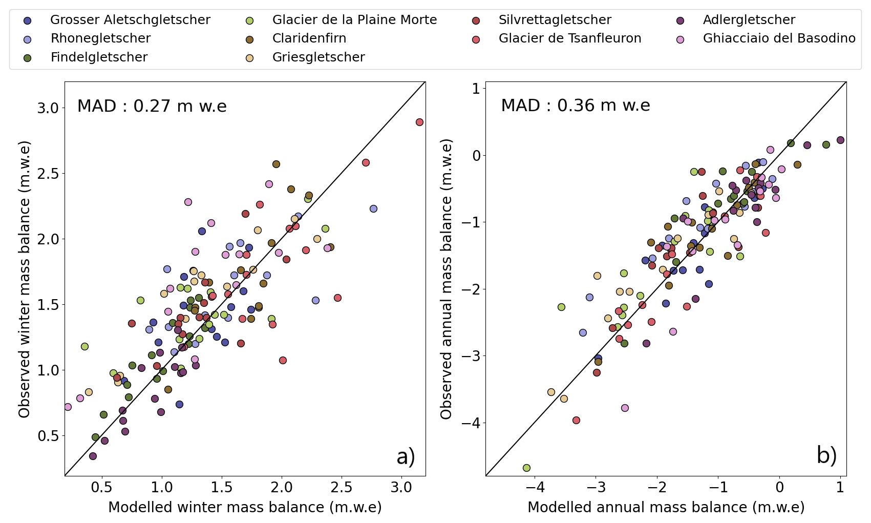
Figure 4 Evaluation of seasonal glacier-wide mass balance. (a) Comparison between modelled and observed winter mass balance. (b) Comparison between modelled and observed annual mass balance.

With a mean absolute deviation (MAD) of 0.27 $\mathrm{m}\mathrm{w}.\mathrm{e}.$ and a bias of −0.08 $\mathrm{m}\mathrm{w}.\mathrm{e}.$ the model slightly underestimates winter mass balance, and with a MAD of 0.36 $\mathrm{m}\mathrm{w}.\mathrm{e}.$ and a bias of −0.05 $\mathrm{m}\mathrm{w}.\mathrm{e}.$ the model provides slightly more negative annual mass balance. These values, together with the data points clustering along the 1:1 line in both cases (Fig. 4), demonstrate a good agreement with observed seasonal mass balances for glaciers calibrated on SCAF observations. Additionally, seasonal glacier-wide mass balance is validated against a second set of 13 glaciers, for which no SCAF observations are available and to which precipitation correction factors have been extrapolated (see Sect. 3.2.4). For these glaciers, the MAD for winter balance is 0.31 $\mathrm{m}\mathrm{w}.\mathrm{e}.$ (bias of −0.02 $\mathrm{m}\mathrm{w}.\mathrm{e}.$), and the MAD for annual mass balance is 0.38 $\mathrm{m}\mathrm{w}.\mathrm{e}.$ (bias of 0.16 $\mathrm{m}\mathrm{w}.\mathrm{e}.$). Despite a small bias towards less negative mass balances than observed, these values confirm the reliability of the extrapolation approach with machine learning. The evaluation against sub-seasonal point mass balance measurements included 19 glaciers, of which 10 relied on extrapolated precipitation correction factors. Evaluation against point measurements is conducted for shorter periods, i.e. up to the weekly scale, providing valuable insights into the accuracy of the model outputs on short time scales and thus the temporal course of modelled mass balance over the summer season. Although daily point measurements are available for some glaciers (Landmann et al., 2021; Cremona et al., 2023), we aggregated such measurements at the weekly scale to reduce measurement uncertainties. Because CRAMPON is an elevation-band type of model, we compare the observed mass balance acquired at the elevation z with the modelled mass balance resulting for the elevation band that includes the elevation z. The standardized mean absolute deviation, calculated as the MAD between modelled and observed values divided by the observed values, is 33 %, confirming the model reliability in providing daily point mass balances (Fig. 5).

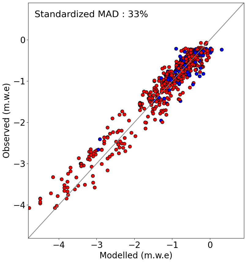
Figure 5 Evaluation of cumulated modelled daily mass balance against point mass balance measurements for periods spanning 7–90 d. Blue dots correspond to locations above the median glacier elevation, and red ones below it.

By binning the individual data points of Fig. 5 into classes of observed mass balance, it becomes clear that the model matches the observations well over the full range of the measurments (Figs. S3 and S4 in the Supplement). A locally increased bias, for example, in the bin with the most negative observed mass balance, may be related to specific conditions at the considered data points but is not sufficiently pronounced to be interpreted in a general sense.

3.4 Uncertainty assessment

To estimate the uncertainty in the modelled mass balance, we account for uncertainties stemming from (a) the geodetic volume change used during calibration, (b) the modelled evolution of the glacier area, (c) the extrapolation of the precipitation correction factor with machine learning, and (d) the presence and effect of supraglacial debris. Uncertainties introduced by different geodetic volume change estimates during calibration are derived by changing the input geodetic volume change used across the available options. Uncertainties arising from the modelled evolution of the glacier area are derived by conservatively varying modelled area change rates by ±50 %. This value covers a broad range of glacier area responses and, hence, considers that our parametrization is rather simple. Uncertainties originating from the extrapolation of the precipitation correction factor with machine learning are derived by varying c_prec by ±0.37, which corresponds to the RMSE found by cross-validation (see Sect. 3.2.4). Uncertainties associated with the presence of supraglacial debris cover are derived by running the model as if there were no debris. The deviation of the mass balance resulting from the different new model runs (a)–(d) from the reference run was statistically evaluated, providing the resulting uncertainties σ_geodetic, σ_area, σ_{extrapolation}, and σ_debris. These uncertainties are considered independent and are combined into an overall uncertainty in daily glacier-wide mass balance for every day as:

$$\begin{array}{}\text{(8)}& {\mathit{\sigma }}_{\dot{b}}=\sqrt{{\mathit{\sigma }}_{\text{geodetic}}^{\mathrm{2}}+{\mathit{\sigma }}_{\text{area}}^{\mathrm{2}}+{\mathit{\sigma }}_{\text{extrapolation}}^{\mathrm{2}}+{\mathit{\sigma }}_{\text{debris}}^{\mathrm{2}}}\end{array}$$

resulting in an average uncertainty in daily mass balance that ranges up to 0.037 $\mathrm{m}\mathrm{w}.\mathrm{e}.{\mathrm{d}}^{-\mathrm{1}}$ with a mean of 0.0026 $\mathrm{m}\mathrm{w}.\mathrm{e}.{\mathrm{d}}^{-\mathrm{1}}$. Uncertainties in inferred Swiss-wide winter and annual mass balance are 0.27 and 0.20 $\mathrm{m}\mathrm{w}.\mathrm{e}.$, respectively. The average uncertainty in the mass balance cumulated over the entire study period is 2.5 $\mathrm{m}\mathrm{w}.\mathrm{e}.$

To test the sensitivity to the modelled glacier surface albedo, we tested two additional scenarios, i.e. by systematically varying the albedo by +25 % and by −25 %. The sensitivity of the resulting mass balance is low, i.e. with a standard deviation between the two scenarios of just 2 % for both winter and annual mass balance. This is not surprising given that the model is tightly constrained with various observational data, thus leaving little room for the albedo parameterization to strongly affect trends in our results.

We compute the mass balance uncertainty at the Swiss-wide scale ${\mathit{\sigma }}_{B_{\text{CH}}}$ as:

$$\begin{array}{}\text{(9)}& {\mathit{\sigma }}_{B_{\text{CH}}}=\sqrt{\sum _i\left({\mathit{\sigma }}_{{\dot{b}}_i}^{\mathrm{2}}\cdot {\displaystyle \frac{A_i}{A_{\text{tot}}}}\right)},\end{array}$$

where ${\mathit{\sigma }}_{{\dot{b}}_i}$ is the mass balance uncertainty for the ith glacier, with its area A_i, and A_tot the total glacier area in Switzerland. Subsequently, we combine the uncertainties in Swiss-wide mass balance (see Eq. 9) and the uncertainties in glacier area as follows to obtain an estimate of the uncertainty in computed ice volume change σ_dV:

$$\begin{array}{}\text{(10)}& {\mathit{\sigma }}_{\mathrm{d}V}=\mathrm{d}V\cdot \sqrt{{\left({\displaystyle \frac{{\mathit{\sigma }}_A}{A_{\text{tot}}}}\right)}^{\mathrm{2}}+{\left({\displaystyle \frac{{\mathit{\sigma }}_{B_{\text{CH}}}}{B_{\text{CH}}}}\right)}^{\mathrm{2}}},\end{array}$$

where σ_A is the estimated uncertainty in glacier area, A_tot the overall glacier area, and B_CH the average mass balance of all Swiss glaciers. This approach provides a first-order uncertainty estimate. However, there remains potential for conducting more rigorous uncertainty assessments.

4 Results and Discussion

4.1 Ice volume change over 2010–2024

According to our results, glaciers in the Swiss Alps lost 15.2 ± 1.6 km³ of ice over the period 2010–2024, i.e. almost 25 % of their volume in 2010 (Fig. 6). This corresponds to an average yearly ice volume loss of 1 km³ of ice. Yearly volume changes range from −2.4 ± 0.16 km³ of ice (in 2022) to a slight volume gain of +0.13 ± 0.09 km³ in 2014 (Fig. 6b). Other years with particularly large losses are 2011, 2017, and 2023, whereas years with only slightly negative mass balance are 2013 and 2021. The region with the largest volume losses over the study period is the Aletsch region, which contributed to almost 30 % of the total ice volume loss in Switzerland. Such high losses for this region are a consequence of below-average annual mass balance (Fig. 7b) combined with the large glacierized area in the region.

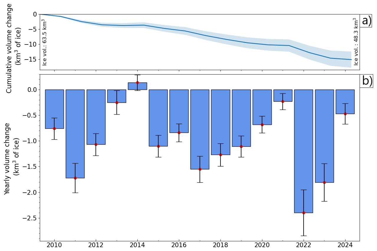
Figure 6 Swiss-wide ice volume change over 2010–2024. (a) The cumulative ice volume change (blue line) over the study period is shown with the respective uncertainty (shaded area). (b) Yearly volume changes (blue bars) with respective uncertainty ranges are shown.

4.2 Seasonal mass balance and climatic drivers

The area-weighted average winter mass balance for the Swiss Alps during the period 2010–2024, taken as the cumulative mass balance between 1 October and 30 April, is 1.27 $\mathrm{m}\mathrm{w}.\mathrm{e}.$ Regional differences in the average winter mass balances are shown in Fig. 7a, where glacier-wide estimates are aggregated on a 20 km × 20 km grid. The largest winter snow accumulation can be observed in central and western Switzerland, with values ranging between 1.5 and 1.9 $\mathrm{m}\mathrm{w}.\mathrm{e}.$ The Aletsch region and the Engadin align with the Swiss-wide average with values around 1.3 $\mathrm{m}\mathrm{w}.\mathrm{e}.$, and the lowest winter mass balances are observed in Valais with values of 0.9–1.2 $\mathrm{m}\mathrm{w}.\mathrm{e}.$

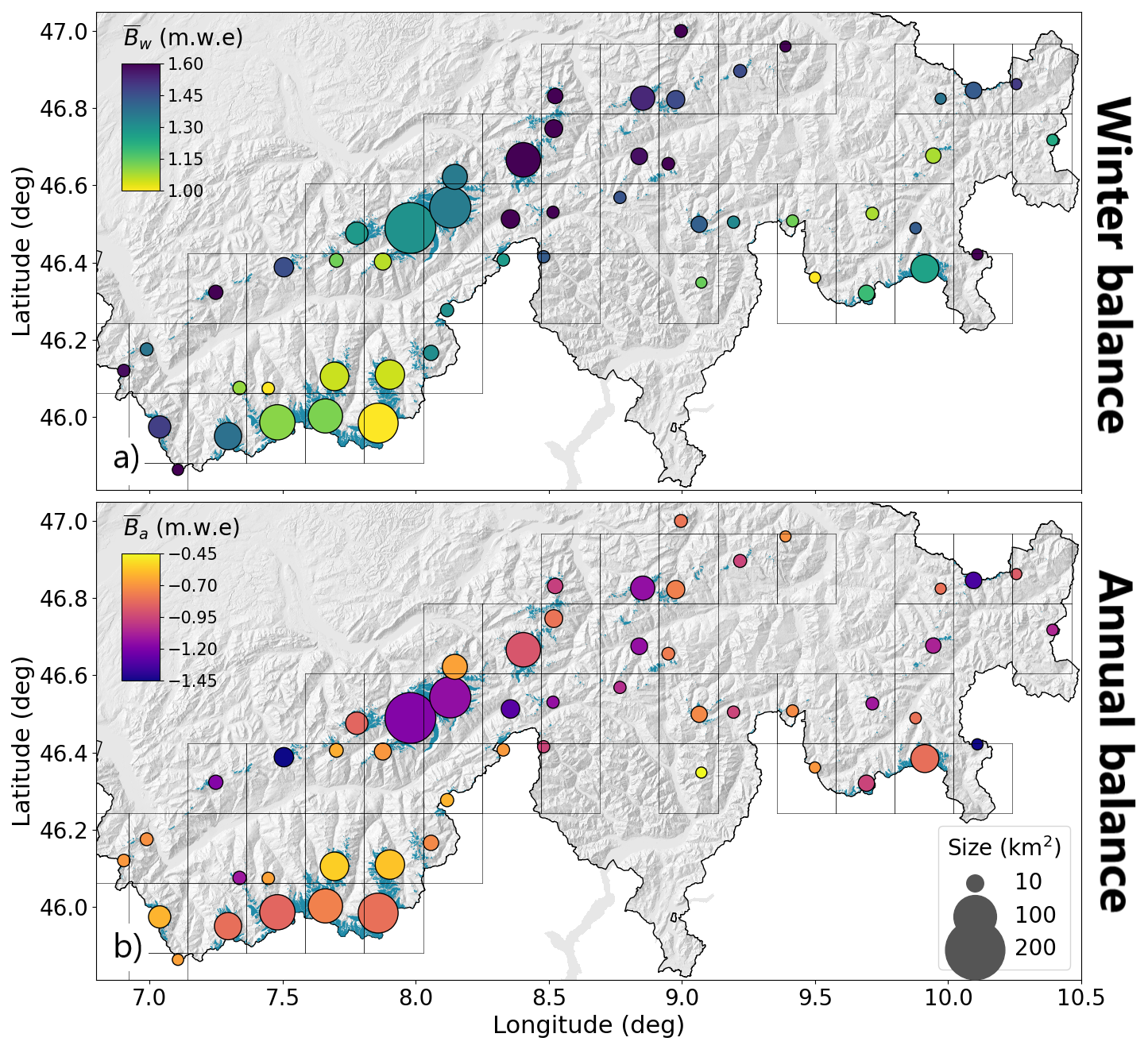
Figure 7 Average seasonal mass balance for the Swiss Alps over 2010–2024. (a) Average winter balance (30 April), and (b) average annual balance (30 September). Glacier-wide values are aggregated over a 20 km×20 km grid with area-weighted averaging, whereby the size of the circles shows the glacierized area within each grid cell.

The area-weighted Swiss-wide average annual mass balance over the study period is −0.95 $\mathrm{m}\mathrm{w}.\mathrm{e}.$, and the aggregated values for the 20 km × 20 km grid range between −0.6 and −1.5 $\mathrm{m}\mathrm{w}.\mathrm{e}.$ (Fig. 7b). Although winter balances correlate well in space, no clear pattern is revealed for the spatial variability of average annual mass balances, whereby neighbouring glaciers and regions present very different values. The only region with a clear signal is the Southern Valais, showing less negative values compared to the Swiss-wide average. This fact has previously been documented by several studies that showed the predominant effect of topographical characteristics on annual balance variations in space, such as the glaciers' mean elevation, as well as the slope, area, and aspect (Kuhn et al., 1985; Hoelzle et al., 2003; Huss et al., 2012; Fischer et al., 2015). Thus, several neighbouring regions in Fig. 7b, which may include glaciers with different topographical characteristics, present diverging average annual mass balances. In contrast, the high spatial correlation for winter balances in Fig. 7a indicates that this variable shows a clear dependence on regional precipitation patterns, while strong topographical controls (e.g. snow redistribution by wind and avalanches) are relevant at the local to glacier scale.

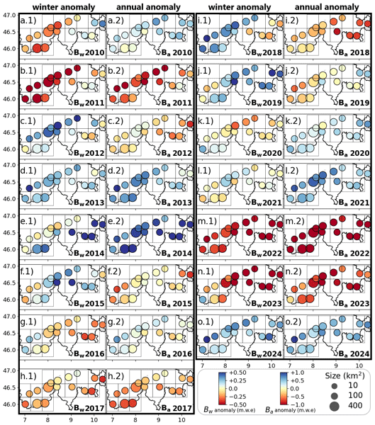
Seasonal mass balances for individual years in the study period are investigated in more detail (Fig. 8), and are compared against temperature and precipitation patterns to further assess the importance of climatic drivers for determining spatio-temporal glacier mass balance variability across Switzerland (Fig. 9). This is achieved by computing seasonal mass balance anomalies for each year with respect to the average seasonal mass balance over the study period, and comparing them to the anomaly of (i) the total precipitation sum over the winter season (October–April) and (ii) the average temperature over summer (May–September). Seasonal mass balance anomalies exhibit different regional signals over the years (Fig. 8), and notably, spatial differences in the anomalies across regions happen to be more accentuated for years with more heterogeneous precipitation distribution (Fig. 9). Furthermore, it can be observed that the spatial pattern in the mass balance variability remains consistent between winter and annual balance in most cases. This consideration is supported by the fact that precipitation anomalies are spatially much more heterogeneous than temperature anomalies and thus have a larger influence on spatial variations of mass balance (Fig. 9). These factors together indicate that the year-to-year spatial variability of mass balance is strongly controlled by regional winter accumulation anomalies.

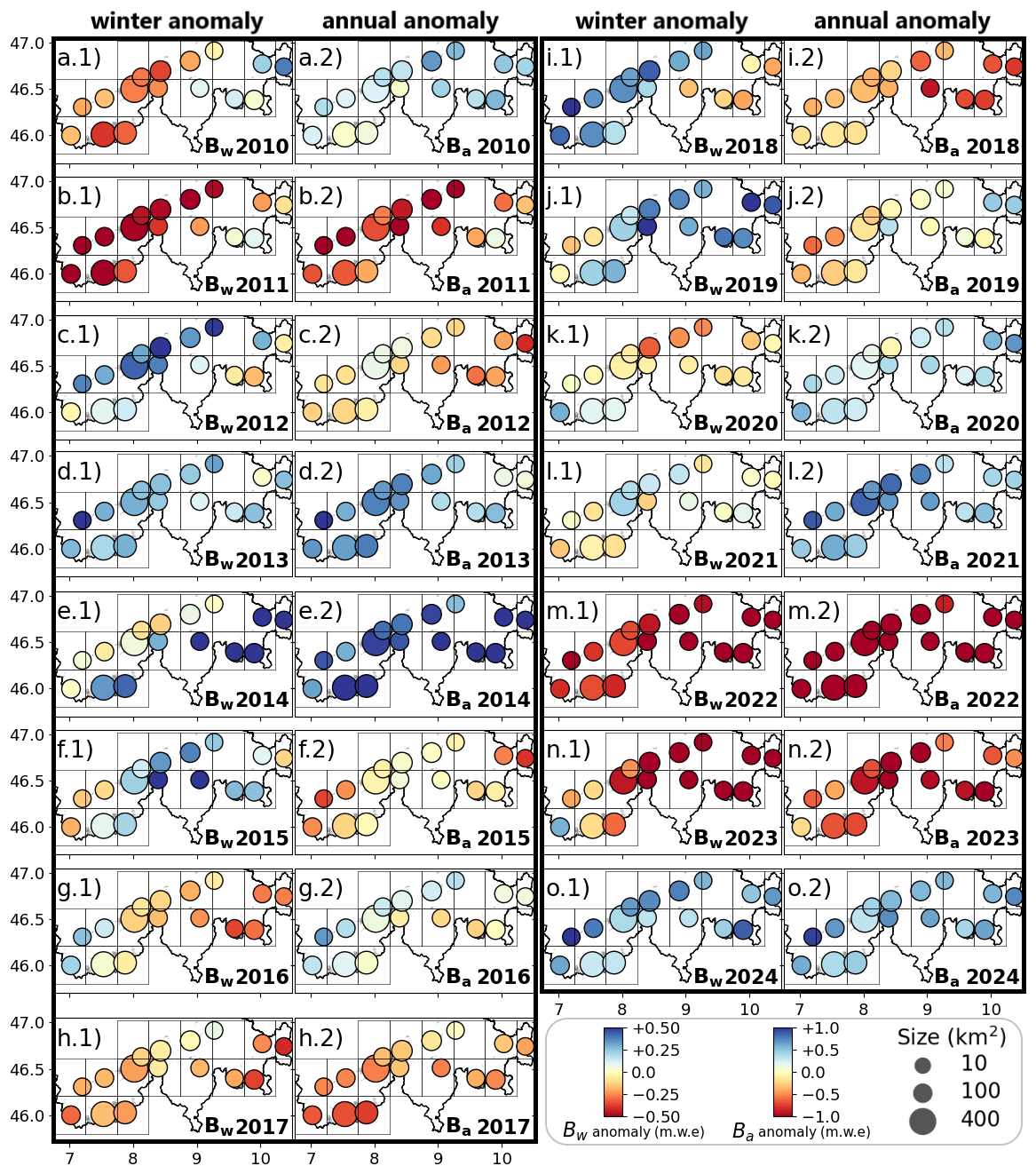
Figure 8 Anomaly of the winter (B_w) and annual (B_a) mass balance with respect to the average winter and annual mass balance over the study period for the years 2010–2024.

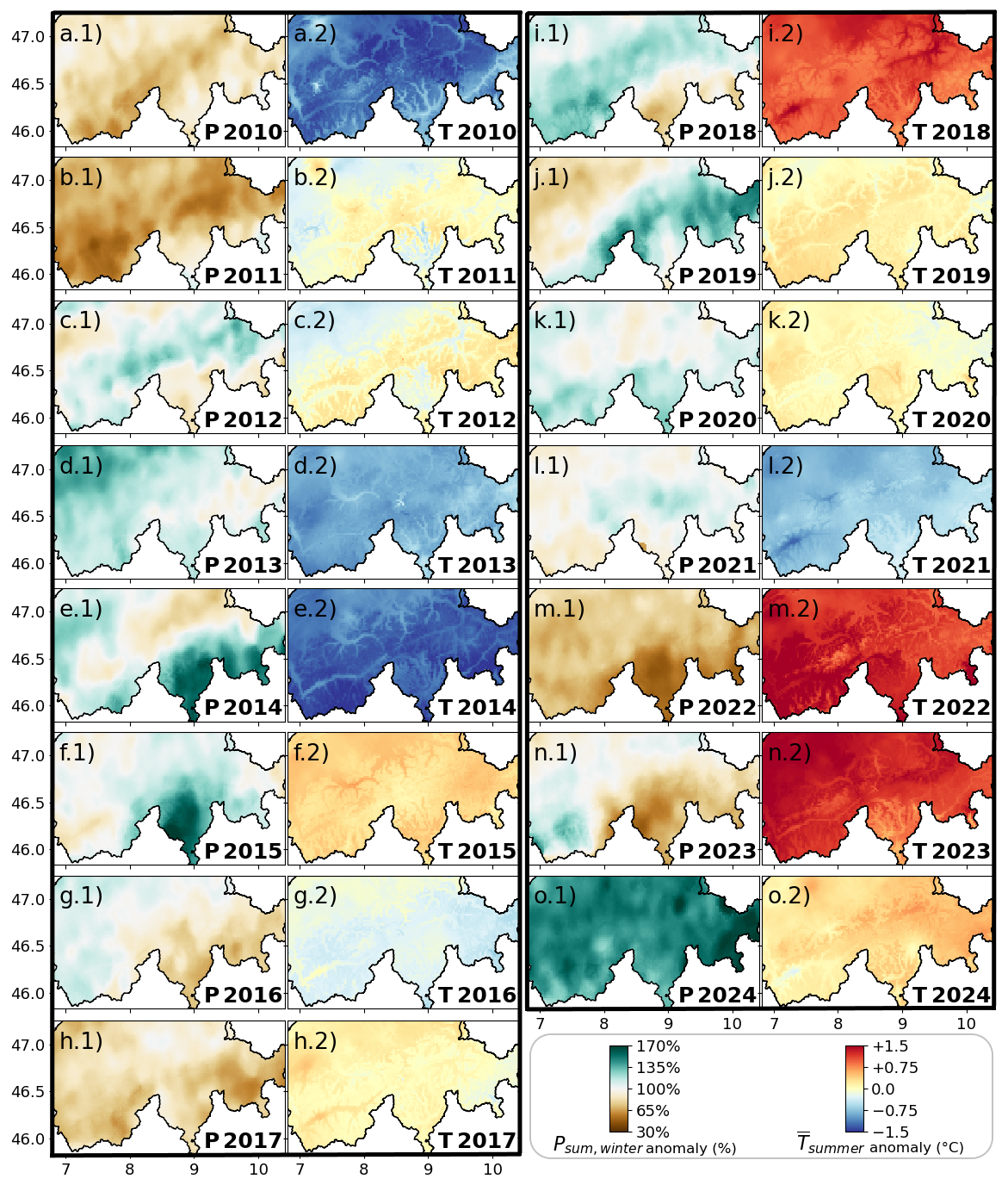
Figure 9 Anomaly of winter precipitation sum (October–April) and mean summer temperature (May–September) with respect to the average values over 2010–2024.

A quantitative comparison between mass balance anomalies and anomalies of the meteorological variables over the study period is shown in Fig. 10. The anomaly of the winter precipitation sum correlates well with the winter mass balance anomaly (r = 0.86), and the anomaly of the mean summer temperature correlates well with the summer mass balance (r = −0.77). The high correlations confirm the predominant influence of temperature and precipitation on determining seasonal mass balance variations. Nevertheless, the spread demonstrates the involvement of other processes, such as the effect of cloudiness and wind-driven turbulent heat exchange, or more localised snow redistribution by wind or avalanches and the influence of Saharan dust on snow albedo. These factors are known to have a significant influence on the balance of glacier mass (Gabbi et al., 2015; Freudiger et al., 2017; Rounce et al., 2021). An interesting aspect is the limited dependence of annual mass balance on the temperature anomaly in the case of mass gain (Fig. 10b). For example, annual mass balances of between 0 and +1 $\mathrm{m}\mathrm{w}.\mathrm{e}.$ can occur with the same air temperature offset. This can be attributed to the pivotal role of the precipitation regime in a given year that does not need to be correlated with the temperature anomaly.

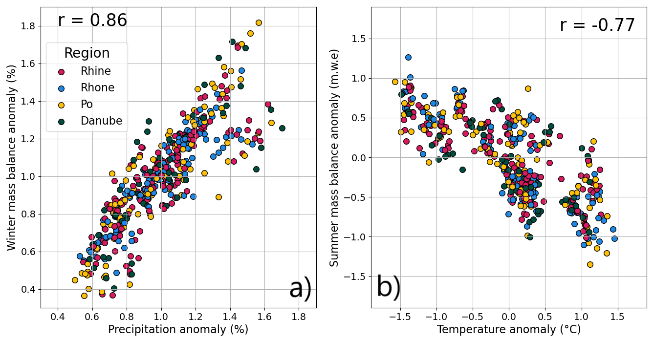
Figure 10 Correlation between mass balance anomalies and the anomalies in meteorological variables for all Swiss glaciers (aggregated on the 20 km × 20 km grid). (a) Winter precipitation anomaly vs. winter mass balance anomaly. (b) Summer temperature anomaly vs. summer mass balance. The colours distinguish the different hydrological basins where the glaciers are located.

4.3 Short-term mass balance variability

Our approach has the advantage of providing mass balance estimates with a high spatio-temporal resolution for all glaciers of the Swiss Alps, enabling us to derive and compare daily mass balances across regions (Fig. 11). In Fig. 11, the daily mass balance is aggregated over the four main hydrological basins in Switzerland (Rhine, Rhone, Po, and Danube), and it is compared for three years, i.e. a year with slightly positive mass balance (2014), an average year (2016), and a highly negative year (2022). In 2014, the mass balance at the end of the year is close to zero for the Rhine and Rhone basins, whereas it is more positive for the Po and Danube basins (Fig. 11a). The lower summer temperatures recorded in 2014 across Switzerland, i.e. by −1 to −1.5 °C with respect to the 2010–2024 average (Fig. 9e.2), reflect the smaller melt rates observed across the four basins in 2014 compared to 2016 and 2022 (Fig. 11). Winter accumulation for 2014, instead, presents larger variations, which closely match the spatial variability of the winter precipitation (Fig. 9e.1). While the Rhine and Rhone basins experienced average winter accumulation, the Po and Danube basins exhibited above-average accumulation, with winter mass balances of more than 2 $\mathrm{m}\mathrm{w}.\mathrm{e}.$ by the end of April. This difference is a key factor leading to slightly positive annual mass balances for the Po and Danube basins in 2014. By comparing the course of the mass balance between 2014 and 2016, it can be observed that for the Rhine and Rhone basins the winter accumulation is similar between the 2 years, and the higher melt rates in 2016 caused by higher summer temperatures are mainly responsible for the more negative mass balance at the end of the year (−0.8 to −0.9 $\mathrm{m}\mathrm{w}.\mathrm{e}.$). This highlights the importance of summer temperatures for driving annual mass losses. The comparison for the Po and Danube basins between 2014 and 2016, instead, shows the impact of favourable conditions both during the winter and the summer season on mass balance. With about twice the accumulation in 2014 and lower summer temperatures, the difference in annual balance between 2014 and 2016 is of more than 1 $\mathrm{m}\mathrm{w}.\mathrm{e}.$ for both basins. In contrast, the year 2022 shows the drastic effect of a year with extremely unfavorable conditions (Berthier et al., 2024; Menounos et al., 2025). This year was characterized by (i) among the lowest winter precipitation sums recorded over most of Switzerland during the study period, (ii) one of the warmest summers (Fig. 9) with the presence of several heatwaves (Cremona et al., 2023), and (iii) a very early start of the melt season (e.g. Voordendag et al., 2023). The combination of these factors led to a fast depletion of the snow cover, leaving large fractions of glacier ice exposed very early in the season, and led to unprecedented ice losses recorded in one year, i.e. with a mass balance of below −2 $\mathrm{m}\mathrm{w}.\mathrm{e}.{\mathrm{yr}}^{-\mathrm{1}}$ for all four basins (Fig. 11) and almost −2.5 km³ of ice wastage in the Swiss Alps (Fig. 6b).

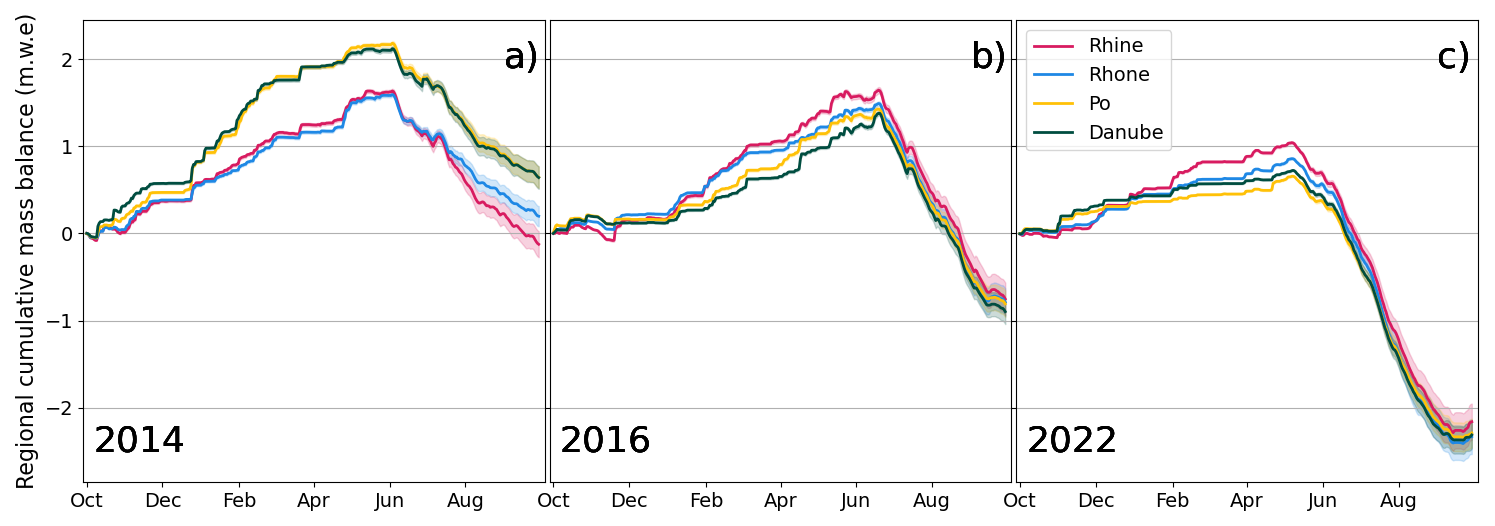
Figure 11 Comparison of daily regional mass balance aggregated over the four main hydrological basins in Switzerland, i.e. Rhine (in pink), Rhone (in blue), Po (in yellow), and Danube (in green), for three years, i.e. a positive year (2014, a), an average year (2016, b), and a negative year (2022, c).

Our daily mass balance time series provides the basis for further assessments related, for example, to changing characteristics of the melt seasons over the years. Here, we assess (i) changes in the length of the melt season, and (ii) changes in the melt rates during summer over the study period. We define the length of the melt season as the number of days between the date with the maximum cumulative mass balance and the date with the lowest cumulative mass balance (both expressed relative to 1 October). No significant trend indicating a lengthening of the melt season can be observed. We also compared the melt rates during the summer months (June, July, and August) to detect the potential intensification of the melt rates. However, also here no significant trend was found. Strong year-to-year fluctuations are present in the inferred variables. These variations override a potentially significant trend over the relatively short time period considered here.

4.4 Comparison to existing approaches and limitations

The comparison between the results of this study based on distributed mass balance modelling constrained with SCAF observations and and those obtained from statistically upscaling the seasonal variability (GLAMOS, 2024c; van Tiel et al., 2026) generally reveals a high agreement, but also points out some differences (Fig. 12a). The Swiss-wide volume change over the study period agrees well for both approaches, with a difference in total volume change of approximately 10 %, which is within the respective uncertainty ranges (see Sect. 3.4 for the derivation of uncertainties). The volume losses found in the present study are slightly less negative. Despite the temporal variations of annual volume changes agreeing well, the systematic difference between the two approaches can be observed in most years, whereby larger differences are present in specific years (Fig. 12a). The most prominent example is 2022 where our results point to less important mass losses compared to extrapolating observed mass balances of that year. Large differences are present also in 2014, 2023, and 2024. The differences between the two approaches in terms of total ice volume loss range between 0.4 and 0.7 km³. Notably, all these years were characterised by non-average conditions, and in some cases, extreme conditions. 2014 and 2024 experienced wet winter seasons, leading to large accumulation amounts, whereas 2022 and 2023 were among the warmest and driest years on record in Switzerland.

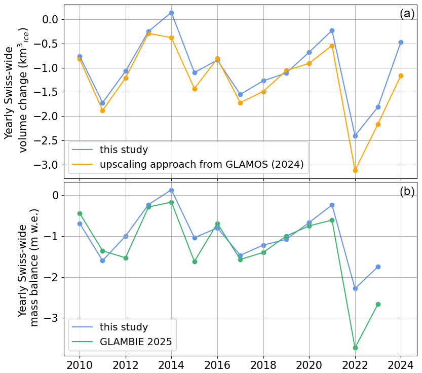
Figure 12 Comparison with existing approaches. (a) Comparison of the yearly Swiss-wide ice volume change between this study (blue) and the upscaling of local mass balance measurements (GLAMOS, 2024c; van Tiel et al., 2026) (orange). (b) Comparison of the yearly Swiss-wide mass balance from this study (blue) and the yearly mass balance for the European Alps from The GLAMBIE Team (2025) (green).

These differences are likely explained by three main factors. The first factor is linked with the methodological differences between the two approaches. Here, we rely on glacier-specific modelling driven by daily meteorological data, in contrast with the more data-driven approach relying on statistical upscaling of seasonal variability inferred from measurements for a subset of about 20 glaciers (see also Dussaillant et al., 2025). Therefore, seasonal and annual mass balance variations are directly determined by meteorological forcing and the optimally constrained model parameters in the present approach, while statistical methods for inferring regional mass change extrapolate measured mass balance anomalies from a small set of observations.

The second factor is associated with data availability. In the present study, we include newly-derived ice volume changes from a large set of digital elevation models covering the study period, while the statistical upscaling data product considered here (GLAMOS, 2024c; van Tiel et al., 2026) relied on longer-term and older geodetic mass balances (Fischer et al., 2015) for inferring glacier-specific mass change trends. This may be responsible for the systematic differences between the data sets as long-term glacier mass changes are given by different data. Additionally, the geodetic estimates from the two approaches cover different periods during which the conditions for glaciers changed considerably with potential consequences on the outputs of the respective approach.

The third factor is linked with the limitations and uncertainties of the respective approaches (see also Sect. 3.4). A limitation of this study is that we assume a constant parameter set over the entire study period, neglecting temporal variations in the parameters that may be driven by processes not accounted for in the model. This, for example, pertains to the albedo effect of Saharan dust, or the influence of other components of the energy balance (e.g. turbulent heat fluxes, long-wave radiation variations). This can especially impact the temporal variability of mass balance and volume change, explaining some of the differences observed in individual years with non-average and even extreme conditions, i.e. in 2014, 2022, 2023, and 2024.

Another limitation is associated with the machine-learning extrapolation approach. In fact, the training data set for the machine-learning model is (i) relatively small, and (ii) biased towards large glaciers. This may lead to a bias in inferred mass balances, especially for small glaciers. Despite these limitations, the evaluation, which also includes small glaciers (about 40 % of considered glaciers are smaller than 1 km²) indicated that the extrapolation approach is also reliable for that size class (see Sect. 3.3). No bias in the resulting mass balance for small glaciers was detected. This confirms the method's reliability, but we suggest keeping in mind such limitations if the presented method is to be applied elsewhere.

The calculation of the initial temperature lapse rate, based on the grid cells around the glacier's centroid (see Sect. 3.2), does not consider the surface type of the cells, which may lead to inaccurate estimates. Our temperature lapse rates range from −6.5 to −4.4 K km⁻¹ with an average value of – 6 K km⁻¹, i.e. slightly lower than the value commonly used in global glacier modelling studies of −6.5 K km⁻¹ (Schuster et al., 2023). While for the large glaciers, the surface type of most grid cells around the glacier centroid corresponds to ice, for small glaciers the surface type may be different, i.e. mostly rock. Thus, the different microclimate could affect the resulting temperature lapse rate. To overcome this challenge, other studies calculated lapse rates directly from pressure levels of gridded climate re-analysis datasets (e.g. Marzeion et al., 2012; Draeger et al., 2024). However, the high-resolution meteorological dataset for Switzerland does not provide the respective information. Also, gridded air temperature in the available data set is not derived from physically-informed modelling that distinguishes between glacier and non-glacier grid cells but is based solely on terrain elevation and interpolation of surrounding weather station data (MeteoSwiss, 2021a). As a result, since most meteorological stations are located below 2500 $\mathrm{m}\mathrm{a}.\mathrm{s}.\mathrm{l}.$, air temperature lapse rates in high mountain areas are inherently poorly constrained. We thus adjust lapse rates during calibration, and we argue that applying a more sophisticated method to estimate their initial values would only have a minor impact.

Another limitation is associated with the rather simplistic parameterizations employed to account for changes in glacier area and the effect of supraglacial debris. Both parameterizations are first-order approximations to account for these effects for the presented regional-scale assessment. We thus do not expect these approaches to exactly match actual processes everywhere, but assume them to be reliable on average. As a consequence, for example, elevation bands near the terminus are likely to lose mass and area with a somewhat lower rate than it is modelled. Nevertheless, since the study focuses on the regional scale, and bearing in mind the relatively short study period considered, we consider these first-order approximations to be reasonable assumptions.

Despite these limitations, our approach has the advantage of relying on the most recent geodetic estimates. In addition, the high resolution of the results presented here, both in time and space, provides an elevation-specified distribution of daily mass balance, which is not available from direct upscaling of glacier mass balance observations. Furthermore, this study models mass balance for every glacier individually, relying on regional remote sensing products and machine learning for extrapolation; thus, estimates for glaciers without direct measurements are likely more reliable.

Additionally, we compared our mass balance estimates with the one from The GLAMBIE Team (2025), derived for the European Alps. Despite the fact that the two datasets do not compare the exact same region, the results are consistent (Fig. 12b). The findings agree with the comparison with local data sets based on upscaling (GLAMOS, 2024c; van Tiel et al., 2026), indicating that the mass balances generally compare well, with the main discrepancies observed in individual years, especially the extreme ones such as 2022 and 2023.

5 Conclusions

In this study, we provide the daily mass balance for the ∼ 1400 glaciers in the Swiss Alps over the period 2010–2024. Relying on a modelling framework and exploiting machine learning techniques for spatial extrapolation, remote sensing observations of the snow-covered area fraction are combined with geodetic volume changes to separate the accumulation and ablation components, and thus better reproduce the seasonal variability of mass balance.

We estimate a total ice volume change over 2010–2024 of −15.2 ± 1.6 km³, i.e. almost 25 % of the ice volume in 2010 was lost in 15 years. Swiss-wide seasonal average mass balances over the study period amount to 1.27 $\mathrm{m}\mathrm{w}.\mathrm{e}.$ for winter and to −0.95 $\mathrm{m}\mathrm{w}.\mathrm{e}.$ for the annual scale, respectively. The spatial variability of seasonal mass balance is further evaluated to capture regional differences, showing a clear pattern for winter accumulation with the highest amounts in central and western Switzerland ranging between 1.5 and 1.9 $\mathrm{m}\mathrm{w}.\mathrm{e}.$ and lowest values are recorded in Valais with values of 0.9–1.2 $\mathrm{m}\mathrm{w}.\mathrm{e}.$ Winter accumulation exhibits high spatial correlation, revealing a strong dependence on precipitation patterns, whereas annual balances ranging between −0.6 and −1.5 $\mathrm{m}\mathrm{w}.\mathrm{e}.$ are less spatially correlated, confirming the predominant effect of local topographical factors on annual balance as already documented in the literature.

The high spatio-temporal resolution of our approach enabled us to better understand the relation between seasonal mass balance and the climatic drivers in the Swiss Alps, underlining the relevance of winter accumulation on the year-to-year spatial variability of mass balance. Furthermore, this study does not rely on direct field measurements for calibration and thus highlights the importance of remote sensing observations to provide reliable estimates of short-term mass balance of unmeasured glaciers at the scale of entire regions. The approach holds substantial potential, and its applicability to other regions worldwide mainly depends on the availability of the input data, i.e. SCAF observations, DEMs, and daily meteorological products. Overall, this suggests that observations of the snow-covered area fraction on glaciers may improve glacier-specific modelling at the large scale.