Mass changes of the Antarctic Peninsula ice sheet and peripheral glaciers, 2007–2021

The Antarctic Peninsula (AP), encompassing the ice sheet and its peripheral glaciers, is a highly dynamic component of the cryosphere that disproportionately contributes to sea-level rise relative to its size. However, a large spread remains between the mass changes estimated using gravimetry, altimetry and the mass budget method. Among these techniques, the satellite (radar or laser) altimetry method has a resolution of, at best, 1 km, which is too coarse to resolve the mountainous landscape of the Peninsula. Therefore, we use digital elevation models (DEMs; 30 × 30 m) to provide an estimate of mass changes across the AP between 2007 and 2021. We combine 476 DEMs derived from SPOT5-HRS satellite images (2006–2008) and 2525 DEMs of the Reference Elevation Model of Antarctica (2020–2022) to map elevation changes for the entire Peninsula. We vertically adjusted each DEM using near-coincident ICESat/-2 laser altimetry measurements. Our observations cover 70 % of the AP Ice Sheet and 60 % of its peripheral glaciers, including regions of the Peninsula poorly studied to date, and reveal a spatially complex pattern of elevation changes. After correction with different models of firn air content and solid-earth response, we find that between 2007 and 2021, the AP Ice Sheet lost 28 ± 6 Gt a⁻¹ while its peripheral glaciers lost 14 ± 3 Gt a⁻¹. For the AP Ice Sheet, our new estimate is 4 to 5 times more negative than the one obtained in IMBIE using altimetry data (−5.2 ± 1.8 Gt a⁻¹ from 2007 to 2019) and in better agreement with gravimetry and the mass budget method. Our study highlights the importance of resolving fine scale elevation changes of glaciers and ice sheets in complex, dynamic coastal areas.

1 Introduction

The Antarctic Peninsula, covering an area of 335 000 km² (Silva et al., 2020), is a mostly narrow and mountainous region, characterized by a high altitude plateau that predominantly feeds marine terminating glaciers (Fig. 1a). The Antarctic Peninsula Ice Sheet (APIS) is surrounded by numerous islands partly covered by ice that are independent from the mainland, referred herein as the peripheral glaciers (Pfeffer et al., 2014). Climate conditions vary greatly across the AP, with mild weather and high snowfall in the west, and drier and colder conditions in the east, where most ice shelves are found (Orr et al., 2008). In the context of climate change, the AP ice masses are responding dynamically. The region encompasses many of Antarctica's rapidly changing glaciers; these changes are often linked to the thinning or breakup of their ice shelves, e.g. Drygalski, Hektoria, and Crane Glaciers (Rott et al., 2002; Rignot et al., 2004; Scambos et al., 2004). Although the APIS constitutes only 4 % of the total area of the whole continent and 0.5 % of the total ice volume (extracted from Pritchard et al., 2025), it represented ∼ 15 % of Antarctica's total glacier mass loss between 1992 and 2020 (Otosaka et al., 2023). Both tidewater and ice shelf tributary glaciers of the AP are projected to significantly contribute to sea-level rise, caused by complex dynamic responses to climate change (Schannwell et al., 2016).

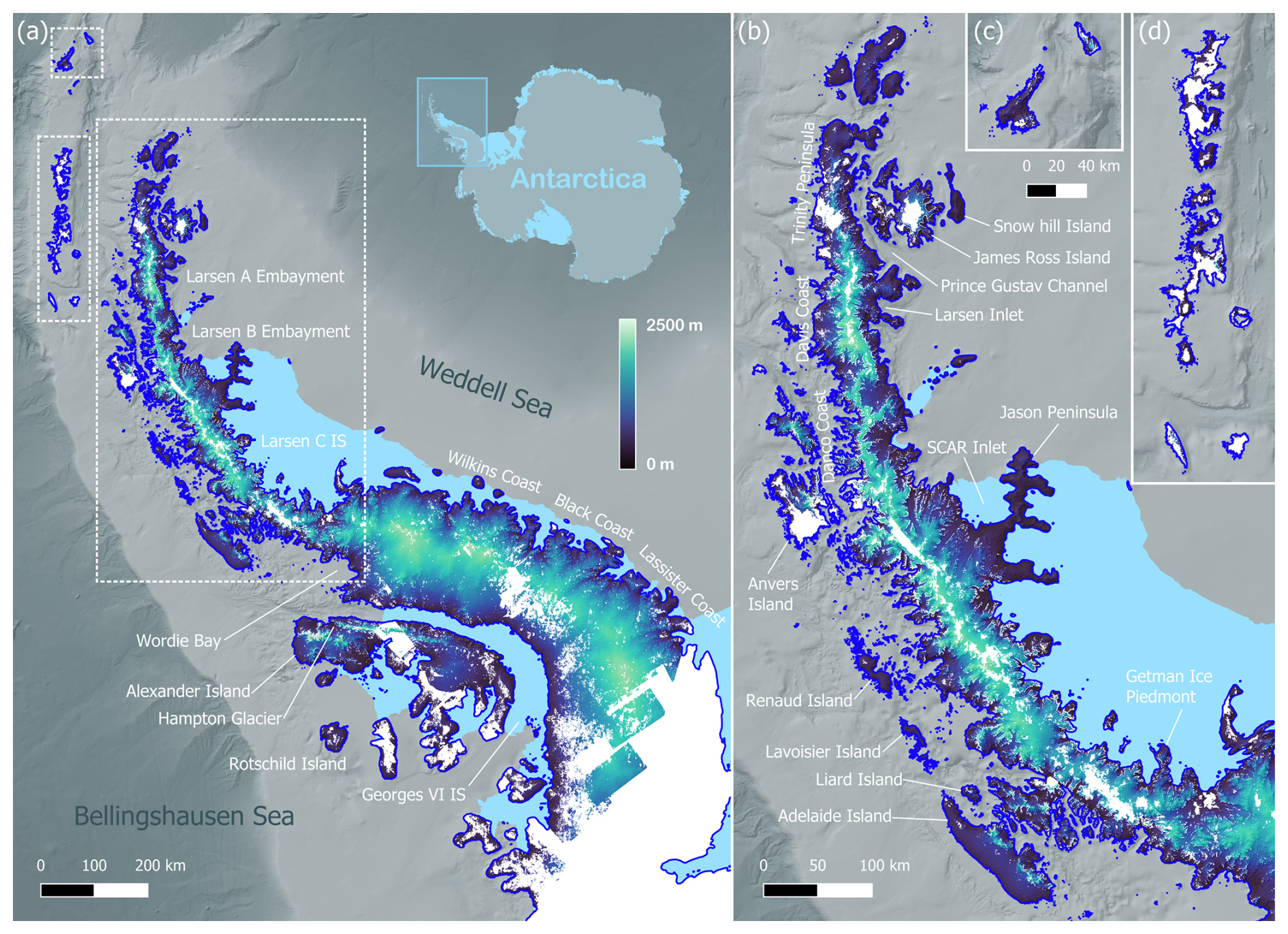
Figure 1 Spatial coverage obtained from SPOT5-HRS archive over the Antarctic Peninsula (2006–2008). Terrain with SPOT5-HRS data coverage colored, while gaps are shown in white. Grounded ice and ice shelves (IS) outlines are plotted as thick blue line and light blue respectively, while the bathymetry is shown as a colored hillshade (Pritchard et al., 2025). (a) shows the SPOT5-HRS DEMs coverage on the entire AP. (b), (c) and (d) correspond to the insets indicated as white boxes on (a), zooming on the northern part of the APIS (b) and the South Shetland Islands (c) and (d). We included the names of the main geographical features cited in the text.

Previous studies have estimated the mass evolution of the APIS at various timescales, from multidecadal (e.g. Nilsson et al., 2022; Rignot et al., 2019) to short-term changes (e.g. Seehaus et al., 2023; Wouters et al., 2015). Three main methods are used to study the mass changes of the polar ice sheets, including the APIS: gravimetry, the mass-budget method (also called the input-output method) and the elevation-differencing method, based on laser or radar altimetry. Estimates have been calculated regularly (e.g. Otosaka et al., 2023; Shepherd et al., 2018) and show a large spread in inferred mass loss, especially for the APIS. For example, over the period 2007–2019, mass changes ranging from −5.2 ± 1.8 Gt a⁻¹ (altimetry) to −41.7 ± 9.5 Gt a⁻¹ (mass budget method) were estimated for this region (adapted from Otosaka et al., 2023). All these methods, providing APIS-wide estimates, do not resolve fine-scale processes.

Elevation differencing has been extensively applied to the AP using sparse satellite altimetry measurements but rarely from digital elevation models (DEMs). The DEM-differencing method has been used to study very localized sites (e.g. Zhao et al., 2017), occasionally providing multidecadal time series (e.g. Kunz et al., 2012). When applied to larger subregions of the AP, it was limited to short time periods (≤ 5 years, e.g. Seehaus et al., 2023; Scambos et al., 2014; Rott et al., 2018). Here, we investigate the mass changes of all AP glaciers using the DEM-differencing method. DEMs can provide elevation information at high spatial resolution (2–100 m) across areas of hundreds to thousands of square kilometers. However, openly available DEM datasets, derived either from optical or radar sensors, are not available at annual resolutions for the entire AP. This is due to frequent and persistent cloud-cover hindering optical acquisitions, and the difficulty of unwrapping the phase of radar images due to the region's steep topography. Depending on the acquisition technique, DEMs have different limitations: radar-based DEMs often have firn penetration biases (Bannwart et al., 2024; Rott et al., 2021), while DEMs from optical stereoscopic imagery are affected by lack of contrast in very dark (e.g. shadows) and very bright (e.g. fresh snow) areas (Noh and Howat, 2015). Furthermore, any elevation differencing method requires the use of external models to correct first-order elevation changes for physical processes that affect surface height but not ice mass. These include firn densification, glacial isostatic adjustment (GIA) and elastic rebound (ELR). The inclusion of these models can introduce large uncertainties into this method.

In this study, we provide a new estimate of the mass changes of the entire AP between 2007 and 2021, covering the APIS and its peripheral glaciers (Hock et al., 2023). We used only optical imagery and laser altimetry to avoid signal penetration effects. We generated nearly complete topography for 2006–2008 from the SPOT5-HRS archive (fifth Satellite pour l'Observation de la Terre, High Resolution Stereoscopic) that we compared to REMA DEMs (Reference Elevation Model of Antarctica, Howat et al., 2022) from 2020–2022. Both stereoscopic datasets were vertically adjusted on near-coincident laser altimetry data (ICESat and ICESat-2–Ice, Cloud, and land Elevation Satellite), resulting in a vertical precision for the elevation difference maps of typically half a meter per year per pixel. We calculated maps of elevation difference rates over the 14-year period 2007–2021 that we corrected with different models of firn air content (FAC), GIA and ELR to obtain mass changes for the entire AP.

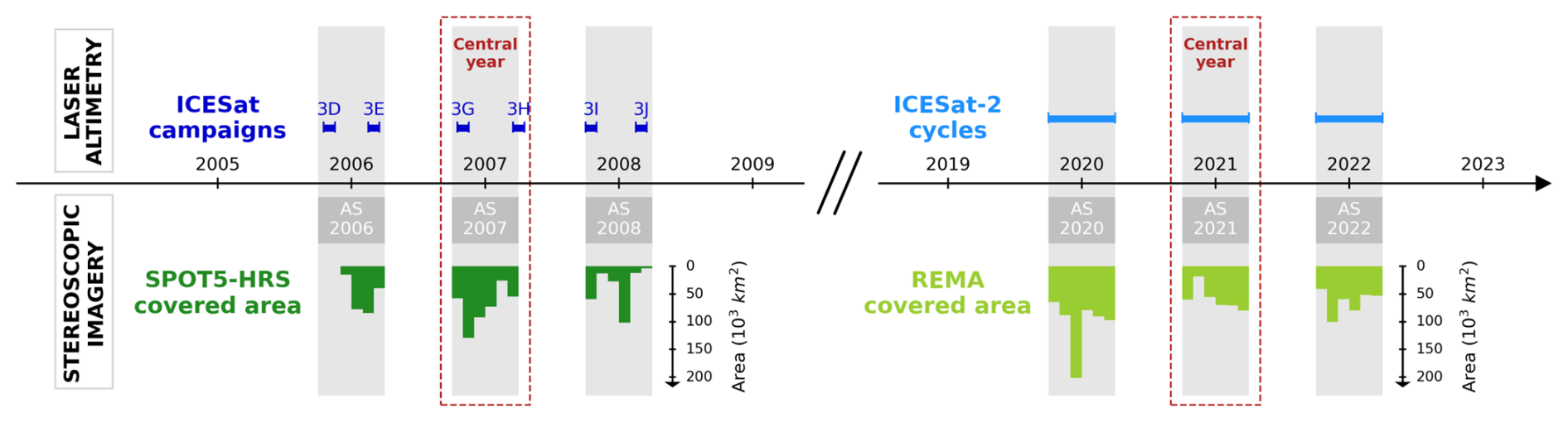
Figure 2 Timeline of the elevation datasets. For the first epoch (2006–2008), monthly SPOT5-HRS covered area is indicated in dark green and ICESat campaigns duration in dark blue. For the second epoch (2020–2022), monthly REMA covered area is indicated in light green and the ICESat-2 extracted periods in light blue. AS stands for austral summer.

2 Data

This study focuses on the elevation and mass changes between two epochs. Each epoch corresponds to three consecutive austral summers, defined as the period from October of the previous year to March of the given year. The first epoch is centered on 2007, including austral summers of 2006, 2007 and 2008, and the second one is centered on 2021, including austral summers of 2020, 2021 and 2022. We used elevation data from two types of measurements, stereoscopic imagery and laser altimetry, defined in the polar stereographic coordinate system (EPSG 3031). Data sources differ between the two epochs: for the first, we used ICESat for laser altimetry and SPOT5-HRS for the DEMs, and for the latter we used ICESat-2 and REMA. The temporal distribution of the elevation datasets is shown in Fig. 2.

2.1 Stereoscopic imagery

2.1.1 SPOT5-HRS archive

SPOT5 is an optical satellite that was operated between May 2002 and March 2015. It was equipped with the HRS sensor that acquired image pairs in panchromatic mode (0.48–0.71 µm). Stereoscopic pairs were acquired in a single pass of the satellite, 90 s apart. The sensor was also characterized by a large 120 km swath and rectangular 5 m × 10 m pixels (along-track x cross-track, Bouillon et al., 2006). As part of the SPIRIT program (SPOT5 stereoscopic survey of Polar Ice: Reference Images and Topographies, Korona et al., 2009), the Antarctic Peninsula was surveyed during the austral summers of 2006, 2007 and 2008 (Fig. 2). The data recorded by HRS used 8-bit encoding, which only allows for 256 different gray-levels. This is one of the main limitations of this sensor in glaciological studies where ice and snow surfaces, that are highly reflective, can produce saturated pixels (Berthier et al., 2023). To help mitigate this effect, during the SPIRIT program, the sensor gains were adapted every week to ensure good contrast over ice sheets surfaces relative to the time of year and latitude. In 2021, all the SPOT5-HRS data archive was made publicly accessible through the CNES Spot World Heritage Program.

2.1.2 Reference Elevation Model of Antarctica

The REMA project was created to produce the first gapless DEM of Antarctica at high spatial resolution (Howat et al., 2019). Sub-meter stereoimages were acquired by four commercially operated satellites: GeoEye-1 (from 2008, 15.2 km swath), WorldView-1 (from 2007, 17.6 km swath), WorldView-2 (from 2009, 16.4 km swath) and WorldView-3 (from 2014, 13 km swath). For each available stereopair, a DEM was generated (Noh and Howat, 2017) at 2 m pixel resolution. Due to the high spatial and radiometric resolution of the stereoscopic images, even areas with low contrast terrains, like snow, ice and shadows, could be measured. Time-stamped DEMs and their associated binary masks (pixel validity) are publicly available at a 2 m pixel resolution (Howat et al., 2022). We used REMA DEMs acquired during the austral summers of 2020, 2021 and 2022. These years were selected because they had the most acquisitions over the AP compared to later years.

2.2 Laser altimetry

2.2.1 ICESat

ICESat was launched by NASA in 2003, primarily to monitor the mass change of the ice sheets (Zwally et al., 2002). Until 2009, elevation data was collected from the GLAS (Geoscience Laser Altimeter System) instrument over Greenland and Antarctica, with a polar orbit up to 88° north and south. Laser pulses of 1064 nm wavelength (infrared) were used to measure surface heights with an along-track sampling interval of 172 m and a footprint diameter of 60 m. Due to unexpected laser malfunctions, the initially continuous operation mode was converted into 9 campaigns of 8 to 37 d every three to six months (Schutz et al., 2005). To match the SPOT5-HRS temporal coverage (2006–2008), we selected the high energy campaigns 3D, 3E, 3G, 3H, 3I and 3J (Fig. 2). We used the GLA12 Records Release 34 ice sheets elevation product (Zwally et al., 2014).

2.2.2 ICESat-2

Building on the legacy of ICESat, the ICESat-2 mission was designed to extend and improve the elevation measurements from space-borne laser altimetry (Markus et al., 2017). The satellite began operations in September 2018 on the same orbit as its predecessor (88° north and south) and is still operational in 2026, with a repeat cycle of 91 d. The Advanced Topographic Laser Altimeter System (ATLAS) carries three pairs of laser beams that measure the surface height, enabling slope effect correction and increasing spatial coverage. The photon counting detectors also improved the along-track spatial sampling to 0.7 m with a footprint diameter of 17 m. For glaciological purposes, we used the ATL06 product Land Ice Elevation at 40 m along track resolution. In line with the epoch of REMA DEMs, we retrieved ICESat-2 data for the austral summers of 2020, 2021 and 2022 (Fig. 2).

2.3 Glacial catchment outlines

We selected four distinct glacier outline datasets for different purposes. Firstly, we used the outlines of glacial catchments and rock outcrops from Silva et al. (2020). We refer to these outlines as SIL20. This dataset includes peripheral glaciers disconnected from the ice sheet and the glacial catchments of the APIS, resulting in a total of 1855 glaciers. Secondly, to ensure that our results are comparable with other studies, we also used three standard outline datasets: the glacial regions from Zwally et al. (2012), hereafter ZWA12, and the Ice Sheet Mass Balance Intercomparison Exercise (IMBIE) glacial regions (Rignot et al., 2013), which both cover only the APIS, and the Randolph Glacier Inventory version 7 (RGI Consortium, 2023), covering the peripheral glaciers.

2.4 Grounding line and bed elevations

We used the BedMap3 (Pritchard et al., 2025) vector product of reconciled grounding lines (Hamish Pritchard personal communication, June 2025). Seafloor and subglacial bed elevations were also extracted from this dataset.

2.5 Firn densification models outputs

To estimate the evolution of the firn air content during the period of study and correct the elevation changes obtained from the DEM-differencing method, we used outputs from four different firn densification models (FDMs) based on various climate and compaction frameworks.

• The first model, referred to as GSFC-FDM, corresponds to the GSFC-FDMv1.2.1 developed by Medley et al. (2022b). It is based on the Community Firn Model (Stevens et al., 2020) and was forced with Modern-Era Retrospective analysis for Research and Applications, Version 2 (MERRA-2, Gelaro et al., 2017).

• The second model, herafter GEMB-FDM, is the Glacier Energy and Mass Balance (GEMB v1.0, Gardner et al., 2023). It was provided by the NASA Jet Propulsion Laboratory and was forced with ERA5 atmospheric re-analysis model (Soci et al., 2024).

• The third model, IMAU-FDM, was developed at the Institute for Marine and Atmospheric Research Utrecht by Veldhuijsen et al. (2023). It was forced by the Regional Atmospheric Climate MOdel (RACMO2.3p2, van Wessem et al., 2018), which was in turn forced with the ERA5 atmospheric re-analysis model (Soci et al., 2024).

• The fourth model, called MAR-FDM, corresponds to the Modèle Atmosphérique Régional version 3.14 (MAR, Fettweis and Grailet, 2024). It was developed by the Liège University and the Grenoble-Alpes University and was also forced with ERA5 atmospheric re-analysis model (Soci et al., 2024).

2.6 Glacial isostatic adjustment models

We selected three paleoclimatic models to correct the changes related to glacial isostatic adjustment. The term GIA is hereafter used to describe the long term crustal viscoelastic response, i.e. related to the deglaciation, and does not include medium and short term evolutions such as since the Little Ice Age. We use one regional model of Antarctic GIA from Whitehouse et al. (2012) and two global models, ICE-6G_D (VM5a) from Peltier et al. (2015) and Caron et al. (2018). We chose to consider GIA models at both regional and global scale to quantify the uncertainty introduced by differences in solid earth models.

3 Methods

The complete analysis workflow of this study is summarized in Fig. 3. First, we prepare the DEMs from SPOT5-HRS and REMA and vertically adjust these with laser altimetry data. Then, we compute elevation difference maps. Finally, we convert volume to mass change, taking into account corrections from GIA, firn densification, and ELR models. The detailed steps are described below.

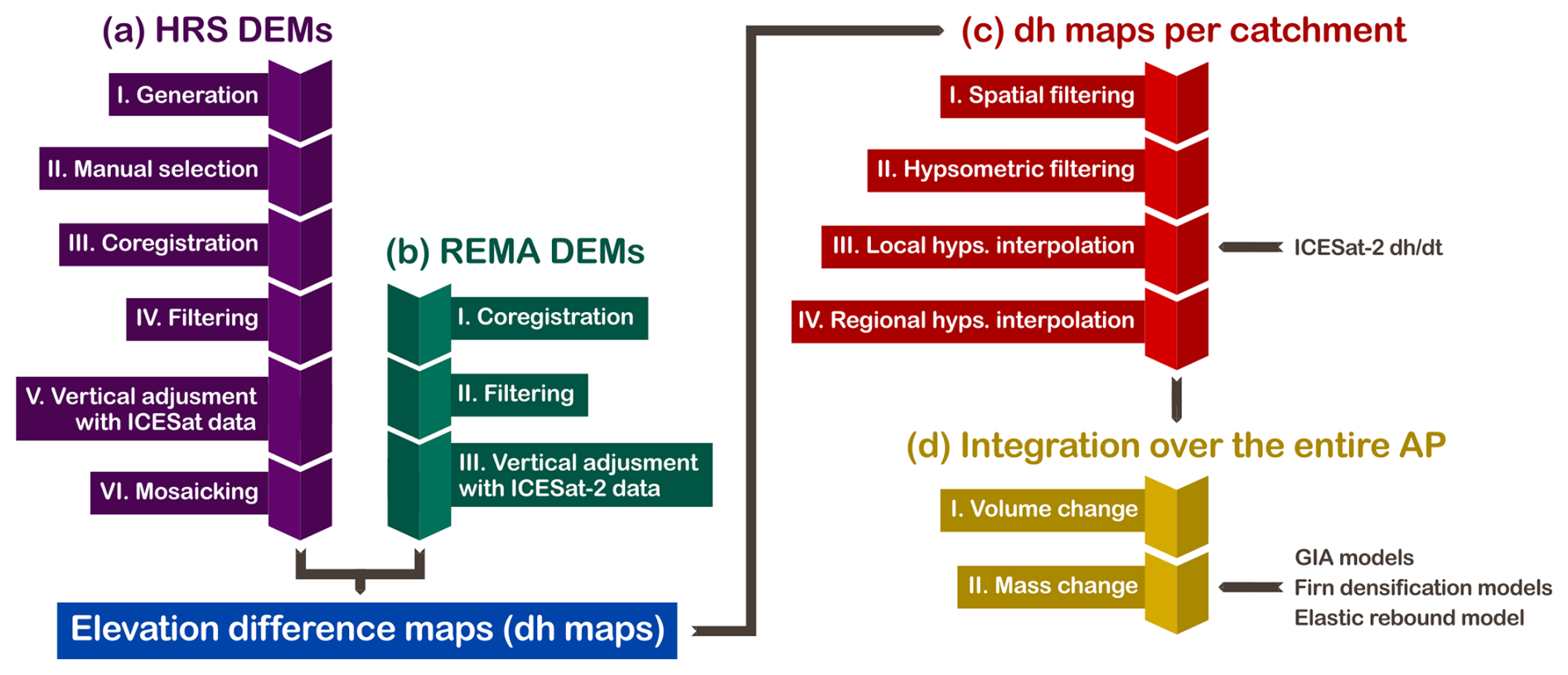
Figure 3 Workflow of the analysis. (a) Processing of the SPOT5-HRS DEMs. (b) Processing of the REMA DEMs. (c) Processing of the elevation difference maps per catchment. (d) Calculations on the entire AP.

3.1 SPOT5-HRS DEM processing

3.1.1 Generation

We used the Ames Stereo Pipeline (ASP, version 3.3.0, Beyer et al., 2018) software developed by NASA to produce DEMs from the optical stereoscopic image pairs. As outlines of the AP vary depending on the dataset considered (up to a few tens of kilometers at the southern limit with west Antarctica), we used the largest dataset extent, SIL20, to identify the image pairs included in the AP. RPC models were attached to the imagery using add_spot_rpc pre-processing routine. We applied the Semi Global Matching algorithm (Hirschmuller, 2008) to correlate the image pairs. We changed the following parameters from the default settings, inspired by Deschamps-Berger et al. (2020): –stereo-algorithm 1 –xcorr-threshold 1 –corr-kernel 7 7 –corr-tile-size 4096 –ip-per-tile 800 –subpixel-mode 9. We generated DEMs with a pixel size of 20 × 20 m using point2dem. Before any further processing, we manually removed the DEMs presenting too few data (less than 20 km²) or too much noise (from visual inspection). The austral summers of 2006, 2007 and 2008 were selected as they contain the majority of the HRS acquisitions of the AP. We obtained a total of 481 HRS DEMs acquired on 110 different dates between 21 December 2005 and 22 March 2008, which we grouped per austral summer. The temporal coverage is shown in Fig. 2 and spatial coverage in Fig. 1, which contains all geographic information hereafter mentioned. The coverage of each austral summer is available separately in Fig. S1 in the Supplement.

3.1.2 Coregistration

All DEMs were coregistered horizontally and vertically to a common reference DEM following Nuth and Kääb (2011) using the Python package xdem (https://doi.org/10.5281/zenodo.19636034, xDEM contributors, 2024). We created the reference DEM by mosaicking the improved TanDEM-X DEM in the northern AP (Dong et al., 2021) with the Copernicus GLO-30 DEM (German Aerospace Center, 2018) edited version of the TanDEM-X DEM in the southern AP. Usually, ice-free terrain of intermediate slope (from 2 to 20°), considered stable, is used to apply the coregistration. However, in the AP, glaciers occupy the vast majority of the surface (> 99 % of the area) and the remaining areas not covered by ice are often small and very steep (Silva et al., 2020). Rock outcrops also become even scarcer in the south of the AP. Therefore, we considered all available elevation data with intermediate slope, including the ice and snow, to perform the coregistration. We identified 20 DEMs with unrealistic horizontal shifts (x- or y-shift larger than median ±3 ⋅ NMAD; normalized median absolute deviation). Three-quarters of these DEMs were successfully re-coregistered with an overlapping HRS DEM, and the remaining ones were kept despite the extreme horizontal shifts, as they provided unique data on flat areas less impacted by a potential coregistration error. We obtained the following mean (μ) and standard deviation (σ) for the x-, y- and z-shifts: μ_x = −0.67 and σ_x = 12.20 m, μ_y = −24.13 m and σ_y = 12.33 and μ_z = −3.60 and σ_z = 5.40 m (Fig. S2).

3.1.3 Filtering

We removed pixels with steep slopes (≥ 50°) that were likely to have large errors (Toutin et al., 2011). We then computed the elevation difference to the TanDEM-X reference DEM as a first coarse estimate to filter out outliers (threshold of 200 m). Then, an asymmetric filter was added to remove very high positive elevation change values (threshold of +20 m). To remove remaining aberrant pixels, we applied a custom percentile-based radial outlier filter. For each pixel, we calculated the 20th (h₂₀) and 80th (h₈₀) percentile within a disk of a radius (r). Defining a threshold (α), pixels with an elevation h such that $|h-h_{\mathrm{20}}|>\mathit{\alpha }$ or $|h-h_{\mathrm{80}}|>\mathit{\alpha }$ were removed. We applied three filters with the following parameters: r = 2 pixels and α = 20 m, r = 5 pixels and α = 50 m, r = 10 pixels and α = 100 m. Details on the effects of each filter can be found on Fig. S4. In total, 16 % of the initial data were removed.

3.1.4 Vertical adjustment on near-coincident ICESat data

The high vertical accuracy and precision of laser altimetry measurements make them a useful tool for correcting the vertical biases of less accurate DEMs. ICESat elevation measurements have already been used to estimate the accuracy of DEMs (e.g. Howat et al., 2019). Thus, we harnessed the temporal overlap of ICESat and HRS DEMs (Fig. 2) to vertically adjust the latter. The spatial sampling was too sparse to use ICESat elevations for horizontal coregistration, but sufficient for a vertical adjustment.

We preprocessed the GLA12 ICESat data identically to Smith et al. (2020). Then, for each HRS DEM, we selected the closest ICESat campaign in time. This resulted in a 52 d maximum time difference between HRS acquisition dates and the central date of ICESat campaigns. We extracted all intersecting points from the chosen campaign. To compute the elevation difference, we bilinearly interpolated the HRS DEM at the coordinates of the ICESat points. We also extracted the slope from the TanDEM-X reference DEM and removed points with a value ≥ 20° to mitigate the effect of slope-induced errors. We imposed a minimum of 20 valid points to compute the mean elevation difference and vertically shift the HRS DEMs by the obtained value. 388 of the 481 initial DEMs were corrected. The mean vertical adjustment, added to the z-shift obtained from the coregistration, was 1.30 m with a standard deviation of 3.05 m (Fig. S2).

Due to the wide spacing of the ICESat tracks (∼ 20 to 30 km) and the brief duration of the acquisition campaigns, 93 DEMs had no simultaneous intersecting ICESat points. Two alternative corrections were considered to vertically adjust the DEMs. First, DEMs that overlapped with an ICESat-adjusted neighbor were coregistered to that neighbor (44 DEMs). Then, DEMs with no ICESat-corrected neighbors were coregistered to the REMA DEM mosaic (see Sect. 3.2), but only using only ice-free terrain with slopes from 2 to 20° (37 DEMs). Any remaining DEMs were removed from the dataset (12 DEMs) with the exception of two DEMs covering the Clarence and Elephant islands (South Shetland Islands archipelago), which were kept uncorrected as they provide unique information on these isolated areas.

Eventually, for each acquisition date, all intersecting HRS DEMs were mosaicked into a single continuous DEM, taking the mean value of overlapping areas. We thus produced 162 mosaics, called HRS segments, covering 76 % of the AP surface. The distribution of time differences between the HRS segments acquisition date and the ICESat campaign center date weighted by area has a mean of −4.8 d and a standard deviation of 37.8 d. Given the negligible mean time difference, we infer that potential seasonal errors introduced by this correction are mitigated when analyzing the whole dataset.

3.2 REMA DEMs processing

3.2.1 Selection, masking and coregistration

For each HRS segment, we identified the overlapping REMA DEMs, acquired in the austral summers 2020, 2021 and 2022 (Fig. 2). We limited the day-of-year difference to ±62 d (2 months) to avoid seasonal errors. For example, a 12 October 2007 SPOT5-HRS DEM would not be compared to a 12 January 2021 REMA DEM as the seasonal difference (3 months) is out of the 2-month maximum interval. We made an exception for the particular case of Drygalski and Hektoria-Green-Evans (HGE) glacier system (Fig. 4c and e). Acknowledging that the extreme elevation changes observed in those areas exceed seasonal effects, we extended the day difference to ±150 and ±125 d respectively in order to get a more complete coverage.

We used the binary mask associated to each REMA DEM to keep only valid pixels i.e. pixels with a 0-flag (no water, nor cloud, nor edge). Then, we coregistered REMA DEMs to the same TanDEM-X reference DEM as the HRS segments (Sect. 3.1.2). REMA DEMs with a x- or y-shift outside of the interval median ± 3 ⋅ NMAD were removed. In total, 3941 DEMs were downloaded, of which 2796 were successfully coregistered. The x-, y- and z-shifts means (μ) and standard deviations (σ) are the following respectively: μ_x = 25.64 m and σ_x = 15.66 m, μ_y = 6.31 m and σ_y = 15.44 m, μ_z = −0.43 m and σ_z = 5.04 m (Fig. S3).

3.2.2 Vertical adjustment with near-coincident ICESat-2 data

Similarly to the SPOT5-HRS DEMs processing, we vertically adjusted the REMA DEMs using near-coincident laser altimetry data, this time from ICESat-2. For 2298 REMA DEMs, we extracted intersecting ICESat-2 data acquired ±31 d apart. We extended the time window to ±62 d for 227 additional DEMs. All ICESat-2 points with a quality flag equal to 0 and a slope value ≤ 20° extracted from the TanDEM-X reference DEM were selected. We set the same threshold of 20 points at minimum as for the SPOT5-HRS DEMs adjustment on ICESat. Then, we bilinearly interpolated the DEMs at each ICESat-2 point and computed the mean elevation difference that was used as a vertical correction. We removed REMA DEMs with a vertical shift larger than 3 NMAD from the median. The mean vertical shift is 0.69 m and the standard deviation is 13.24 m (Fig. S3). We combined all the processed REMA DEMs into a mean mosaic that was used as a stable terrain reference DEM (Sect. 3.1.2), covering 90 % of the AP surface.

3.3 Elevation difference maps processing

3.3.1 Differencing and filtering

We derived all pairwise elevation difference maps (dh maps) possible between the two elevation datasets SPOT5-HRS and REMA, respecting the maximum 62 day-of-year difference, and obtained 8381 dh maps. We converted the elevation differences to rates of elevation change (dh $/$ dt maps) by dividing the dh map by the time difference between the two austral summers considered (between 12 to 16 years). To remove remaining aberrant values, we first applied a spatial filter to all the dh $/$ dt maps, inspired by Hugonnet et al. (2021). For each pixel, the 20th (dh $/$ dt₂₀) and 80th (dh $/$ dt₈₀) percentile were calculated within a disk of a radius (r). We set the radius to 5 pixels and the threshold (β) to 0.5 m a⁻¹. Pixels with a dh $/$ dt value larger than dh $/$ dt₈₀+β or lower than dh $/$ dt₂₀−β were excluded. Then, we implemented a filter based on the binning of dh $/$ dt values against elevations extracted from the TanDEM-X reference DEM, independently for each catchment from the SIL20 outlines. The latter is called hypsometric signal and represents the relationship between elevation change rates and elevations at catchment scale. To extract a clear hypsometric signal, we duplicated the dh $/$ dt maps dataset on which we applied a more restrictive spatial filter (radius of 20 pixels and threshold of 1 m a⁻¹). For each catchment, we collected all this strictly spatially filtered dh $/$ dt data and distributed it according to 50 m elevation bins. We computed the mean and standard deviation of each bin and retained values within mean ± 7 ⋅ std. Non-robust statistics were used to account for the effect of valid but outlying values on the metrics, which is essential for further volume calculations. Then, we applied this hypsometric filter on the less strictly spatially filtered dh $/$ dt maps cropped to the catchment outlines. Figure S5 illustrates the effects of the spatial and hypsometric filters on an example catchment. Eventually, we merged all the dh $/$ dt data available for each catchment. In areas with different dh $/$ dt estimations, we used the median value, less sensitive to potentially remaining outliers. The obtained dataset covers 66,7 % of the total area of the AP and is shown on Fig. 4.

3.3.2 Glacier outlines editing

Based on the observation of the elevation difference rates maps here produced and on the BedMap3 grounding line vector product, we manually edited the grounding line (marine terminating glaciers) or terminus (land-terminating glaciers) of 61 catchments from SIL20 outlines. This enabled to more accurately delineate grounded ice before further calculations. We also separated the SIL20 catchments into the peripheral glaciers and the APIS. The two domains defined are very similar to the RGI 7 (peripheral glaciers) and to the IMBIE and ZWA12 outlines (APIS). This, and the fact that the outlines of SIL20 were manually corrected, consolidated our choice of using them as primary outlines.

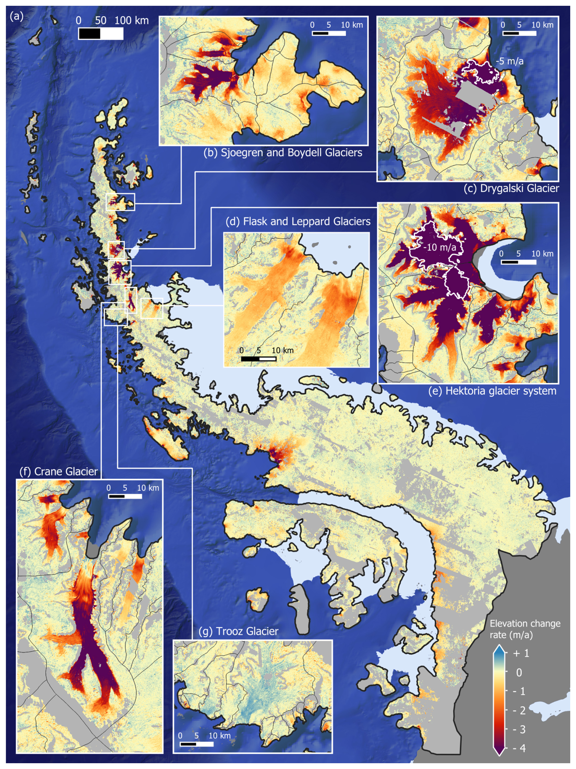
Figure 4 Elevation change rates over the Antarctic Peninsula between 2007 and 2021. Five catchments are highlighted in the insets (b) to (f), with SIL20 catchment outlines plotted in thin black lines. On (c) and (e), the white line indicates the −5 and −10 m a⁻¹ delimitation. The background oceanic hillshade and the ice shelves outlines come from BedMap3 (Pritchard et al., 2025).

3.3.3 Interpolation

The HRS segments and REMA DEMs, even if close to providing complete coverage when aggregated (76 % and 90 % coverage, respectively), do not support a dh $/$ dt dataset covering the entire AP. As complete dh $/$ dt maps are required for further volume and mass changes computations, we included a spatial interpolation step. To add elevation change information where dh $/$ dt map were missing, we extracted elevation data from ICESat-2 matching the same time constraints as for the REMA DEMs extraction (±62 d apart from the HRS DEM acquisition date) for each HRS segment. We computed the elevation difference rate $\mathrm{dh}/\mathrm{d}{t}_{IS\mathrm{2}}$ between HRS and ICESat-2. We grouped all the data per catchment and removed pixels outside of mean ± 7 ⋅ std.

We then focused on hypsometric methods (McNabb et al., 2019), using first a local hypsometric method to fill the uncovered areas. For each catchment, we calculated again the hypsometric signal per 50 m elevation bins. To do so, we averaged the hypsometric signals coming from: (1) the dh $/$ dt maps between REMA and HRS DEMs, (2) the dh $/$ dt_IS2 points between HRS DEMs and ICESat-2 data. We extracted the elevation of empty pixels from the TanDEM-X reference DEM used previously. Eventually, we considered the mean dh $/$ dt value of the corresponding elevation bin to fill the missing data. For 30 catchments representing 3 % of the total study area, no dh $/$ dt data was available. We applied a regional hypsometric method to estimate the elevation change on those catchments: we extracted an AP-scale hypsometric signal considering all dh $/$ dt data available that was used to fill the last voids (see Fig. 5a).

3.4 Volume and mass changes

To obtain rates of elevation change that reflect glacier evolution, several corrections have to be applied. As commonly done in ice-sheet mass changes studies (e.g. Smith et al., 2020, Sanchez Lofficial et al., 2025), we considered the three following corrections: firn density changes (dh${}_{\mathrm{FAC}}/\mathrm{d}t$), glacial isostatic adjustment (${\mathrm{dh}}_{GIA}/\mathrm{d}t$) and the elastic rebound (${\mathrm{dh}}_{\mathrm{ELR}}/\mathrm{d}t$). These corrections are summarized into Eq. (1), where dh $/$ dt represents the elevation difference rates obtained from the initial dh $/$ dt maps and dh${}_{\mathrm{ice}}/\mathrm{d}t$ corresponds to the corrected elevation difference rates. The latter directly reflects ice changes and can be expressed in meters of ice per year (m_ice a⁻¹).

$$\begin{array}{}\text{(1)}& {\mathrm{dh}}_{\mathrm{ice}}/\mathrm{d}t=\mathrm{dh}/\mathrm{d}t-{\mathrm{dh}}_{\mathrm{FAC}}/\mathrm{d}t-{\mathrm{dh}}_{\mathrm{GIA}}/\mathrm{d}t-{\mathrm{dh}}_{\mathrm{ELR}}/\mathrm{d}t\end{array}$$

First, we corrected elevation changes related to the evolution of the firn density. A common variable used to characterize it is the firn air content (FAC). The spatial and temporal evolution of the FAC can be modeled thanks to firn densification models (FDMs). However, large discrepancies exist between the FDMs employed, within the scheme, the climatic forcing and the results produced (Sanchez Lofficial et al., 2025). Therefore, we used the outputs of 4 different FDMs (Sect. 2.5): GSFC-FDM, GEMB-FDM, IMAU-FDM, MAR-FDM. For each of them, we extracted the mean FAC over the three austral summers for the two epochs of study and computed the difference to obtain the FAC change dh${}_{\mathrm{FAC}}/\mathrm{d}t$ over 2007–2021. We spatially extrapolated the dh${}_{FAC}/\mathrm{d}t$ maps on areas with missing data (Fig. S6).

Then, we removed the effect of the glacial isostatic adjustment using three GIA models (Sect. 2.6). As for the FAC correction, we computed the elevation change independently for each GIA model before averaging (Fig. S7). Eventually, we estimated the elastic rebound from the solid Earth caused by current ice changes using the LoadDef code developed by Martens et al. (2019). We used the corrected mass changes (without the elastic correction) with a spatial resolution of 900 m as the input load map and set the parameters to the default settings. More precisely, we kept the Preliminary reference Earth model from Dziewonski and Anderson (1981), commonly used as a reference for solid earth parameters in geodesy studies.

Figure 5 shows dh $/$ dt maps including the uncorrected elevation change and the applied corrections. To calculate volume changes, we integrated the elevation change rates over the areas defined by the four outline datasets used in the study (SIL20; ZWA12; IMBIE and RGI7, see Sect. 2.3). To calculate mass change, we multiplied the corrected volume changes by the ice density (917 kg m⁻³), as they reflect ice changes.

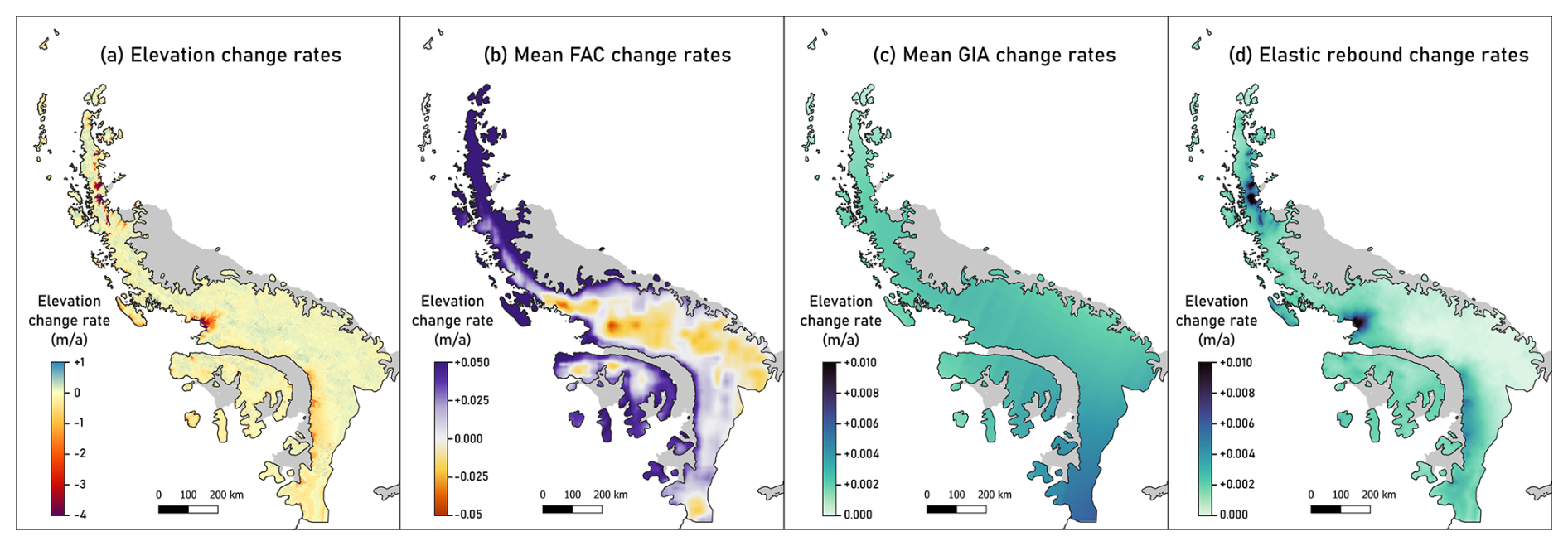
Figure 5 Complete elevation change rates map and the elevation corrections applied, 2007–2021. (a) Interpolated elevation change rates map, (b) Mean FAC changes obtained from the four firn densification models, (c) Mean GIA changes calculated from the three GIA models, (d) Solid earth elastic rebound changes computed with LoadDef. The GIA correction is the only one that is not specific to the period 2007–2021. SIL20 outlines are indicated in black and ice shelves (Pritchard et al., 2025) in grey.

3.5 Uncertainty quantification

To estimate the volume change uncertainty, we considered several sources of uncertainty, assumed independent, summarized in Eq. (2). We consider that the uncertainties related to the area and the ELR are negligible in comparison to other sources. ${\mathit{\sigma }}_{{\stackrel{\mathrm{‾}}{\mathrm{dh}}}_{\mathrm{FAC}}/\mathrm{d}t}$ and ${\mathit{\sigma }}_{{\stackrel{\mathrm{‾}}{\mathrm{dh}}}_{\mathrm{GIA}}/\mathrm{d}t}$ represent the elevation change rate uncertainty induced by the corresponding corrections. Separating the elevation change rates into the observed elevation change rates dh${}_{\mathrm{obs}}/\mathrm{d}t$ and the interpolated elevation change rates dh${}_{\mathrm{interp}}/\mathrm{d}t$, we define two distinct associated uncertainties, ${\mathit{\sigma }}_{{\stackrel{\mathrm{‾}}{\mathrm{dh}}}_{\mathrm{obs}/\mathrm{d}t}}$ and ${\mathit{\sigma }}_{{\stackrel{\mathrm{‾}}{\mathrm{dh}}}_{\mathrm{interp}/\mathrm{d}t}}$. A_tot and A_obs correspond to the total area and the area covered with dh${}_{\mathrm{obs}}/\mathrm{d}t$ maps, respectively.

$$\begin{array}{}\text{(2)}& \begin{array}{rl}{\mathit{\sigma }}_{d{V}_{\mathrm{ice}}/\mathrm{d}t}^{\mathrm{2}}& =({\mathit{\sigma }}_{\mathrm{d}{V}_{\mathrm{obs}}/\mathrm{d}t}^{\mathrm{2}}+{\mathit{\sigma }}_{\mathrm{d}{V}_{\mathrm{interp}}/\mathrm{d}t}^{\mathrm{2}})+{\mathit{\sigma }}_{\mathrm{d}{V}_{\mathrm{FAC}}/\mathrm{d}t}^{\mathrm{2}}+{\mathit{\sigma }}_{\mathrm{d}{V}_{\mathrm{GIA}}/\mathrm{d}t}^{\mathrm{2}}\\ & =A_{\mathrm{obs}}^{\mathrm{2}}\cdot {\mathit{\sigma }}_{{\mathrm{dh}}_{\mathrm{obs}}/\mathrm{d}t}^{\mathrm{2}}+(A_{\mathrm{tot}}-A_{\mathrm{obs}}{)}^{\mathrm{2}}\cdot {\mathit{\sigma }}_{{\mathrm{dh}}_{\mathrm{interp}}/\mathrm{d}t}^{\mathrm{2}}\\ & +A_{\mathrm{tot}}^{\mathrm{2}}\cdot ({\mathit{\sigma }}_{{\mathrm{dh}}_{\mathrm{GIA}}/\mathrm{d}t}^{\mathrm{2}}+{\mathit{\sigma }}_{{\mathrm{dh}}_{\mathrm{FAC}}/\mathrm{d}t}^{\mathrm{2}})\end{array}\end{array}$$

Ultimately, we estimate the mass changes uncertainty as ${\mathit{\sigma }}_{\mathrm{d}M/\mathrm{d}t}^{\mathrm{2}}={\mathit{\rho }}_{\mathrm{ice}}\cdot {\mathit{\sigma }}_{\mathrm{d}{V}_{\mathrm{ice}}/\mathrm{d}t}^{\mathrm{2}}$, with ρ_ice=917 kg m⁻³.

To quantify the uncertainty of the observed elevation changes ${\mathit{\sigma }}_{\stackrel{\mathrm{‾}}{\mathrm{dh}}/\mathrm{d}{t}_{\mathrm{obs}}}$, we applied the method of Hugonnet et al. (2022) that models and propagates autocorrelated elevation change errors. We used the difference between coincident DEMs as an error proxy, instead of the commonly-used differences over static surfaces that can rely on acquisitions of any date, due to the lack of such static surfaces on the AP. Two DEMs acquired within close dates should have near zero elevation changes, thus their elevation difference is a common proxy for errors. We identified multiple coincident pairs of HRS DEMs (13) or REMA DEMs (23), acquired up to five days apart and with a common area of at least 1 km². Then, we computed the standard deviation of the elevation difference for all these HRS and REMA pairs, as a measure of the per-pixel random error of each sensor, ${\mathit{\sigma }}_{{\mathrm{dh}}_{\mathrm{HRS}}}$ and ${\mathit{\sigma }}_{{\mathrm{dh}}_{\mathrm{REMA}}}$ respectively. Those values account twice for the error as pairs of DEMs are considered, so we divided them by $\sqrt{\mathrm{2}}$ before further calculations. To derive the average per-pixel random error of the dh maps between HRS and REMA DEMs, we combine the two errors previously calculated considering them independent, such that ${\mathit{\sigma }}_{{\mathrm{dh}}_{\mathrm{obs}}}^{\mathrm{2}}={\mathit{\sigma }}_{{\mathrm{dh}}_{\mathrm{HRS}}}^{\mathrm{2}}+{\mathit{\sigma }}_{{\mathrm{dh}}_{\mathrm{REMA}}}^{\mathrm{2}}$. We obtained the following values: ${\mathit{\sigma }}_{{\mathrm{dh}}_{\mathrm{HRS}}}=\mathrm{3.92}$ m, ${\mathit{\sigma }}_{{\mathrm{dh}}_{\mathrm{REMA}}}=\mathrm{4.06}$ m and ${\mathit{\sigma }}_{{\mathrm{dh}}_{\mathrm{obs}}}=\mathrm{5.64}$ m.

To constrain the autocorrelation of elevation errors, we derived empirical variograms of the elevation differences of the coincident DEMs from Dowd's median estimator (Dowd, 1984) using the Python package xdem. These variograms, which describe the correlation of errors between two points as a function of their distance, were averaged to get a mean variogram representing each sensor, HRS and REMA. We then modeled the two mean empirical variograms as the sum of two Gaussian and a spherical function (Figs. S8 and S9) to represent the nested autocorrelation structure often observed in elevation data and critical to robust error propagation for volume changes (Rolstad et al., 2009; Hugonnet et al., 2022). HRS elevation errors were correlated by 100 %–20 % until 100 m, then by 20 %–5 % until 200 m, then by less than 5 % until 5 km. REMA elevation errors were correlated by 90 %–10 % until 100 m, then by 10 %–5 % until 200 m, then by less than 5 % until 2 km. We then used the above models to propagate uncertainties spatially from pixel to area into uncertainties of the mean elevation change ${\mathit{\sigma }}_{{\stackrel{\mathrm{‾}}{\mathrm{dh}}}_{\mathrm{obs}}}$ over a defined area. To this end, we derived the numbers of effective samples $N_{{\mathrm{eff}}_{\mathrm{HRS}}}$ and $N_{{\mathrm{eff}}_{\mathrm{REMA}}}$ from the two variogram models following Hugonnet et al. (2022). We propagated the uncertainties coming from the two sensors as ${\mathit{\sigma }}_{{\stackrel{\mathrm{‾}}{\mathrm{dh}}}_{\mathrm{obs}}}^{\mathrm{2}}={\mathit{\sigma }}_{{\mathrm{dh}}_{\mathrm{HRS}}}^{\mathrm{2}}/N_{{\mathrm{eff}}_{\mathrm{HRS}}}+{\mathit{\sigma }}_{{\mathrm{dh}}_{\mathrm{REMA}}}^{\mathrm{2}}/N_{{\mathrm{eff}}_{\mathrm{REMA}}}$. Ultimately, ${\mathit{\sigma }}_{{\mathrm{dh}}_{\mathrm{obs}}}$ was divided by the period of study (14 years) to obtain ${\mathit{\sigma }}_{{\stackrel{\mathrm{‾}}{\mathrm{dh}}}_{\mathrm{obs}}/\mathrm{d}t}$.

Then, we applied a leave-block-out cross-validation method (e.g. Le Rest et al., 2014; Roberts et al., 2017) to estimate the uncertainties that arise from the interpolation, annotated ${\mathit{\sigma }}_{{\stackrel{\mathrm{‾}}{\mathrm{dh}}}_{\mathrm{interp}}/\mathrm{d}t}$. We considered the 709 catchments from the SIL20 outlines with a dh${}_{\mathrm{obs}}/\mathrm{d}t$ coverage larger than 80 % (44 % of the AP surface). For each of them, we created artificial gaps that were then filled following the same methodology as in the data processing, i.e. using the local hypsometric interpolation when possible, and otherwise the regional hypsometric interpolation. To create gaps, we isolated elevation bands of different widths and central elevations, determined from the TanDEM-X reference DEM, on the dh${}_{\mathrm{obs}}/\mathrm{d}t$ map. First, this enabled to better reproduce the shape of our existing data gaps than removing pixels at random coordinates. Second, by varying the width and the central elevation of the hypsometric band removed, we created data gaps ranging from 0 % to 100 %. For each artificial gap generated, we then derived the mean of the difference between interpolated and initial dh${}_{\mathrm{obs}}/\mathrm{d}t$, which served as an error proxy for our spatially-integrated elevation differences over interpolated areas.

We grouped all the means obtained by percent of missing data and, from their distribution, derived the mean and a robust dispersion metric, (84th percentile–16th percentile)$/\mathrm{2}$. The mean accounts for a possible bias introduced by the interpolation, whereas the robust dispersion metric represents the spread around the mean value generated by the interpolation. We modeled the mean with a piecewise-defined affine function, first constant to 0 until 40 % of gaps, then linear reaching the value of 0.06 m a⁻¹ at 100 % of gaps and we fitted a 3° polynomial curve to the series of robust dispersion metrics obtained (Fig. S10). The sum of the mean of the mean and the robust dispersion metric of the mean was then used to estimate the interpolation uncertainty. In other words, given a gap percentage over a catchment, we extracted the corresponding uncertainty ${\mathit{\sigma }}_{{\stackrel{\mathrm{‾}}{\mathrm{dh}}}_{\mathrm{interp}}/\mathrm{d}t}$ from the modeled curves.

Finally, we estimated the uncertainties of the FAC (${\mathit{\sigma }}_{{\stackrel{\mathrm{‾}}{\mathrm{dh}}}_{\mathrm{FAC}}/\mathrm{d}t}$) and GIA (${\mathit{\sigma }}_{{\stackrel{\mathrm{‾}}{\mathrm{dh}}}_{\mathrm{GIA}}/\mathrm{d}t}$) corrections based on the standard deviation between the elevation changes obtained with the different models. We assume conservatively that these uncertainties are fully correlated at the scale of the AP, and thus use this value at every scale (pixel, catchment, whole region). Regarding the elevation change rate uncertainties, we consider ${\mathit{\sigma }}_{{\stackrel{\mathrm{‾}}{\mathrm{dh}}}_{\mathrm{interp}}/\mathrm{d}t}$ fully correlated and apply the method described above to the entire AP, and ${\mathit{\sigma }}_{{\stackrel{\mathrm{‾}}{\mathrm{dh}}}_{\mathrm{obs}}/\mathrm{d}t}$ fully independent (Figs. S8 and S9). Uncertainties are then reported as ±2σ (95 % confidence interval).

4 Results

4.1 Antarctic Peninsula

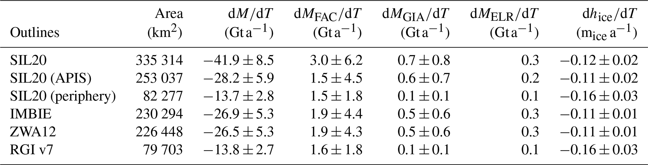
In Table 1, we report our mass change estimates for the period 2007–2021, calculated over several regions defined by different outlines data sets listed in Sect. 2.3. Over the similar ZWA12 and IMBIE outlines, we obtain mass changes of −26.5 ± 5.3 and −26.9 ± 5.3 Gt a⁻¹. For the peripheral glaciers, whose outlines are in the RGI 7 database, we obtained mass changes of −13.8 ± 2.7 Gt a⁻¹. Finally, using the SIL20 outlines that include both the ice sheet and the peripheral glaciers with an updated grounding line, we derived a total mass change of −41.9 ± 8.5 Gt a⁻¹, equivalent to a sea-level contribution of 0.12 ± 0.02 mm a⁻¹ (2.8 % of the 2007–2021 sea-level rise calculated from the Aviso product).

Table 1 Mass and ice elevation changes for the four outline datasets over the period 2007–2021. For each outline dataset, the following variables are indicated: the area encompassed, the total mass changes ($\mathrm{d}M/\mathrm{d}T$), the mass changes from the GIA, FAC and ELR corrections ($\mathrm{d}{M}_{\mathrm{FAC}}/\mathrm{d}T$, $\mathrm{d}{M}_{\mathrm{GIA}}/\mathrm{d}T$ and $\mathrm{d}{M}_{\mathrm{ELR}}/\mathrm{d}T$ respectively) and the ice elevation changes (${\mathrm{dh}}_{\mathrm{ice}}/\mathrm{d}T$). SIL20 catchments were divided into APIS outlet glaciers and peripheral glaciers.

Despite rapidly thinning grounded outlet glacier tongues, wide portions of the AP are close to balance (Figs. 4 and 5a). This is especially noteworthy on the high-altitude center plateau as well as for various locations along the coast (e.g. Larsen C, Wilkins Coast). Mass losses are concentrated in a small number of glaciers that exhibit intense thinning. Most of them are located in the northeastern part (Larsen A & B Embayments, Larsen Inlet), in the mid-southern part (Wordie Bay and along the George VI Ice Shelf) and on the peripheral islands (e.g. Adelaide, Liard, James Ross Islands). Several areas also present coherent thickening patterns, including the northwest of the APIS (Davis Coast), parts of the Jason Peninsula in the northeast and along the Black and Lassister Coasts in the southeastern part.

4.2 Regional scale

Patterns of ice elevation changes differ from region to region. To identify regional differences in the ice elevation changes, we used the four regions from the ZWA12 outline to estimate the ${\mathrm{dh}}_{\mathrm{ice}}/\mathrm{d}t$ hypsometric signal of each of them. The results obtained are presented in Fig. 7, revealing large differences between the regions. For all of them however, mass loss is concentrated at elevations below 800 m. The largest contrast between low and high elevations is found in Region 24 (Fig. 7a), vastest of all regions. Here, the elevation change dh${}_{\mathrm{ice}}/\mathrm{d}t$ shifts from very negative values at low elevation, to significantly positive values above 1200 m. The most negative dh${}_{\mathrm{ice}}/\mathrm{d}t$ values are found between 50 and 150 m and reach −0.72 m_ice a⁻¹ on average. Below 50 m, the scarce zones are dominated by less negative dh${}_{\mathrm{ice}}/\mathrm{d}t$ signal.

Regions 25 and 26 (Fig. 7b and c) show similar dh${}_{\mathrm{ice}}/\mathrm{d}t$ signals and elevation distributions. In both cases, elevations follow a two-peak distribution, one at low elevations (0–600 m) and another at high elevations (1500–2000 m). Contrary to Region 24, the most negative dh${}_{\mathrm{ice}}/\mathrm{d}t$ signal is observed in the lowest elevation bin (0–50 m), reaching a mean of −1.29 m_ice a⁻¹ in Region 25 and −1.06 m_ice a⁻¹ in Region 26. The dh${}_{\mathrm{ice}}/\mathrm{d}t$ signal then gradually increases towards a close-to-zero elevation change rate at the highest elevations. For these two regions, a few glaciers at low elevations have a thickening signal which dominates the third quartile range. For example, considering only elevations below 800 m, Trooz Glacier (Region 25, Fig. 4g) presents a mean ±2σ ice elevation change rate of +0.32 ± 0.26 m_ice a⁻¹. This value, more positive than the mean ice elevation change rate over all elevations of the catchment (+0.06 ± 0.8 m_ice a⁻¹, Fig. 6), highlights low elevation thickening. In Region 25, the negative peak of the dh${}_{\mathrm{ice}}/\mathrm{d}t$ first quartile between 800 and 1000 m is caused by ice-dynamical mass loss of Fleming Glacier. Similarly, the very negative signal at low elevations is largely due to this glacier. In Region 26, the large difference between the mean and the median dh${}_{\mathrm{ice}}/\mathrm{d}t$ below 1200 m of elevation reveals the presence of extremely negative dh${}_{\mathrm{ice}}/\mathrm{d}t$ values that bring down the mean to −1.06 m_ice a⁻¹. Indeed, this region includes the majority of the rapidly thinning glaciers, which reach local minimum elevation change rates of −17.21 m_ice a⁻¹ at Hektoria Glacier, −14.25 m_ice a⁻¹ at Drygalski Glacier, and −6.63 m_ice a⁻¹ at Crane Glacier. Region 27 (Fig. 7d) contains a large area at high elevations, and has a slightly positive mass changes of 1.2 ± 0.4 Gt a⁻¹. This mass gain arises from positive dh${}_{\mathrm{ice}}/\mathrm{d}t$ signals observed at all elevations over the region. The amplitude between the first and third quartiles is particularly limited and remains below 0.32 m_ice a⁻¹. It is the only region exhibiting statistically significant mass gain over the study period.

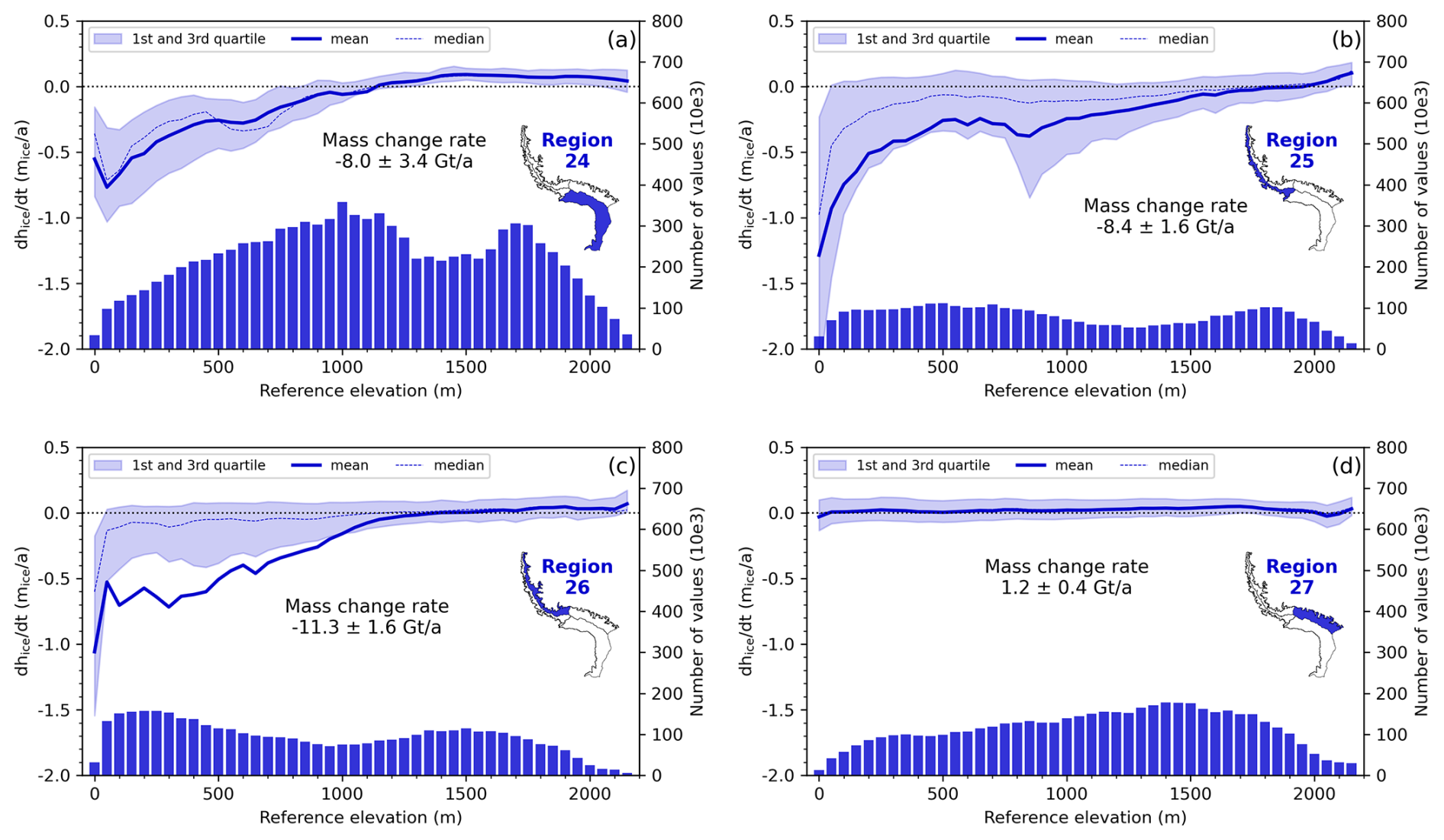
Figure 6 Mean ice elevation change rate of AP glaciers, 2007–2021. The value of the mean ice elevation change rate of 22 catchments is highlighted. Positive mean ice elevation change rates are indicated in blue, negative until −2.00 m a⁻¹ in orange and below in magenta. SIL20 catchment outlines are indicated in black and ice shelves (Pritchard et al., 2025) in grey. The distribution of mean $d{t}_{\mathrm{ice}}/\mathrm{d}t$ is shown in the bottom left corner. The number of catchments is indicated above each column if it is less than three. The 31 catchments presenting the highest mass losses are outlined in blue, with a continuous (≥ 60 % data coverage) or dashed (< 60 % data coverage) line.

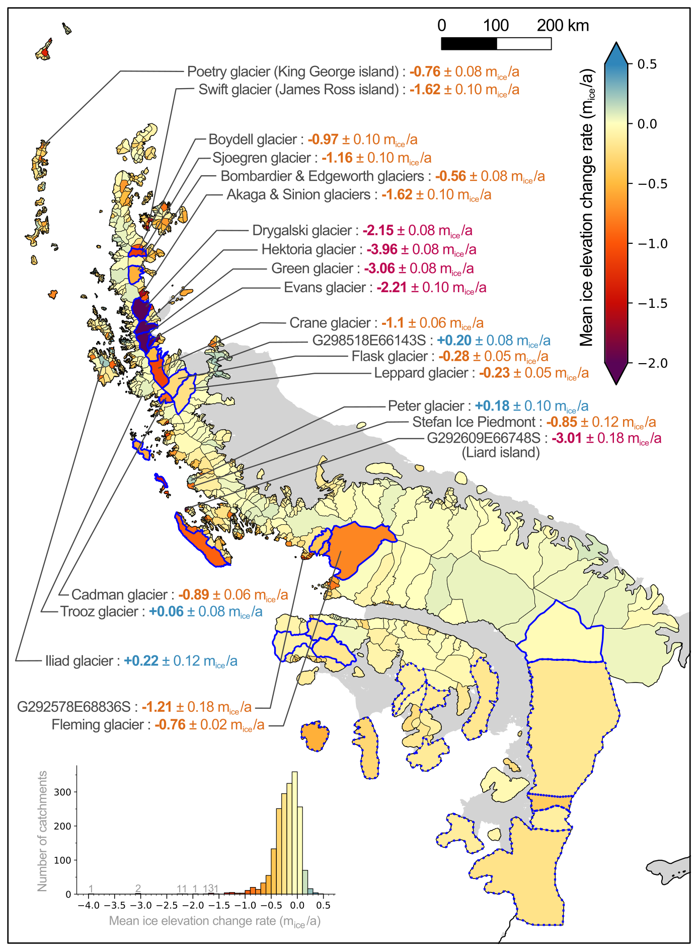
Figure 7 Hypsometric signal of ice elevation changes over AP main regions. For each region from the ZWA12 outline (a)–(d), the histogram at the bottom shows the distribution of elevations over the region. The distribution (median, mean, 1st and 3rd quartiles) of ice elevation change rates per elevation bin are plotted at the top.

We used the division of SIL20 catchments into peripheral glaciers and APIS catchments to document differences between the two domains. The mean dh${}_{\mathrm{ice}}/\mathrm{d}t$ of peripheral glaciers is −0.16 ± 0.03 m_ice a⁻¹, significantly more negative than the rate of −0.11 ± 0.02 m_ice a⁻¹ for APIS (see Table 1). The peripheral glaciers contain more areas at low elevations (between 0 and 500 m), which correspond to the elevations with the most negative dh${}_{\mathrm{ice}}/\mathrm{d}t$ signal (Fig. S11). Thus, if APIS catchments represent 75 % of the total area, they account for −28.2 ± 5.9 Gt a⁻¹, i.e. 67 % of the total mass loss, whereas peripheral glaciers, covering 25 %, account for −13.7 ± 2.8 Gt a⁻¹, i.e. 33 % of the total mass loss.

4.3 Glacier scale

The mean ice elevation change rate for selected catchments from the SIL20 outline dataset is shown in Fig. 6. It highlights the diversity of ice elevation change patterns at a very local scale (< 10 km). Adjacent catchments can present opposite changes, such as Stefan Ice Piedmont (−0.85 ± 0.12 m_ice a⁻¹) and Peter Glacier (+0.18 ± 0.10 m_ice a⁻¹). The Jason Peninsula presents a clear thickening pattern (e.g. G298518E66143S Glacier: +0.20 ± 0.08 m_ice a⁻¹) while its northern tip exhibits dh${}_{\mathrm{ice}}/\mathrm{d}t$ as negative as −0.78 ± 0.10 m_ice a⁻¹. The east-west gradient in the north of the AP is also clearly visible, with very negative mean dh${}_{\mathrm{ice}}/\mathrm{d}t$ in the Larsen A & B Embayments, Larsen Inlet and Prince Gustav Chanel (east) facing close to equilibrium catchments along the Danco and Davis Coasts (west). Thanks to the high spatial resolution of the dh${}_{\mathrm{ice}}/\mathrm{d}t$ maps, small glaciers (e.g. G292609E66748S (Liard island), 15 km², and G292578E68836S, 21 km², see Fig. 6) can be observed and analyzed, including local spatial patterns inside the catchment.

A small number of glaciers accounts for the majority of the AP mass changes. Of all catchments, 24 show a significant (2−σ) thickening signal. They cover 21 % of the total area, and account for a mass gain of 3.0 ± 0.5 Gt a⁻¹. To the contrary, 338 catchments show a significant (2σ) negative mean dh${}_{\mathrm{ice}}/\mathrm{d}t$. They cover 42 % of the AP and correspond to a mass loss of −38.6 ± 2.4 Gt a⁻¹. The remaining 1507 catchments, that do not present a significantly positive or negative ice elevation change rate, cover 37 % of the AP total area, representing a mass change of −6.2 ± 2.8 Gt a⁻¹. Considering the cumulative series of mass changes, we observe that 31 catchments, outlined on Fig. 6, generate 80 % of the total mass loss (−33.6 ±6.0 Gt a⁻¹). They range between −5.39 ± 2.2 Gt a⁻¹ (G289555E73912S, feeding the southern part of Georges VI Ice Shelf) and −0.2 ± 0.04 Gt a⁻¹ (Jorum Glacier). The spatial distribution of these major contributors highlights the predominance in terms of mass losses of the northeastern part of the AP (Sjoegren, Bombardier-Edgeworth, Drygalski, Hektoria, Evans, Jorum, Crane, Flask and Leppard Glaciers, from north to south). It also emphasizes the importance of taking into account the peripheral glaciers. Adelaide, Lavoisier and Renaud Islands are listed among the 31 catchments losing most mass, as well as several catchments from Alexander Island.

5 Discussion

5.1 Spatial patterns and spatial variability

5.1.1 Comparison to other studies

We compared our dh$/\mathrm{d}t$ maps to those from previous studies, on the APIS (Fig. 8) and on the peripheral glaciers (Fig.  9), selecting the closest time period available when possible. These studies are based on different acquisition techniques, thus presenting different coverages, noise and spatial resolutions. They also cover different time periods, which durations range between 4 to 15 years. This spatial comparison highlights the differences and similarities between the studies but also the advantages and drawbacks of each technique.

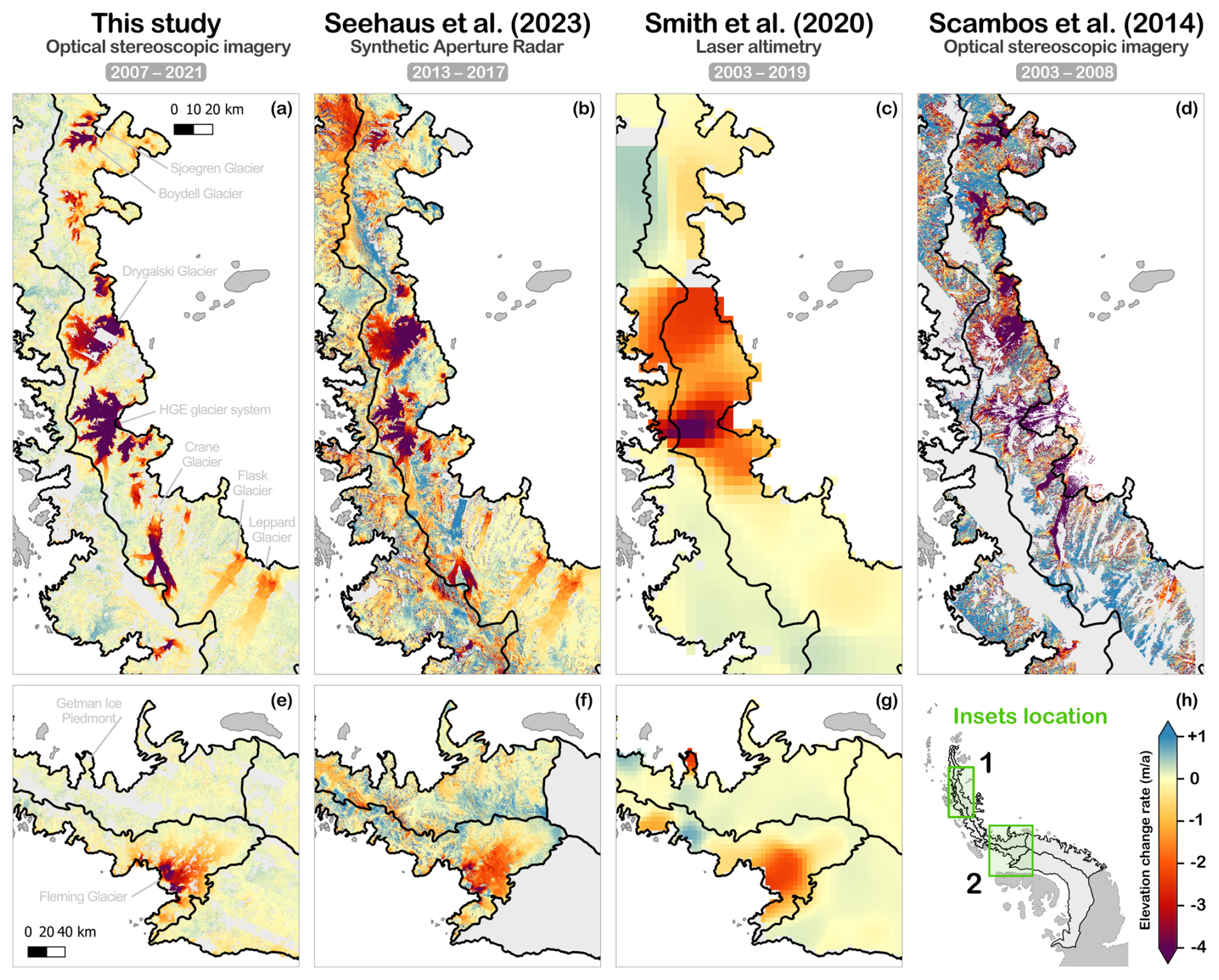
Figure 8 Spatial comparison of elevation change rates maps on selected regions of the APIS. The results from four different studies (this study, Seehaus et al. (2023), Smith et al. (2020) and Scambos et al. (2014)) are compared over two different sites, on panels (a)–(d) and (e)–(g) respectively. The location of the sites is indicated on the last panel (h). The same color scale is used for all maps, but the spatial scale is different for the two sites. The ZWA12 outlines are plotted in black. Note that the elevation change rates map from Scambos et al. (2014) covers only the northern APIS, which does not include the second site of comparison. Note also the different time periods.

Focusing on the APIS (Fig. 8), we compared our results to the three following studies: Seehaus et al., 2023 (Synthetic Aperture Radar or SAR), Smith et al., 2020 (laser altimetry) and Scambos et al., 2014 (optical stereoscopic imagery). Over the APIS, the glaciers presenting extreme thinning rates, such as Drygalski Glacier and HGE glacier system, are clearly visible in all studies (Fig. 8a–d). Similarly, the spatial pattern of intense thinning of a large part of the Fleming Glacier and slight thickening in the upper part of the catchment is observed by all three studies that cover it (Fig. 8e–g). However, many differences in the observed patterns arise, underlying the difficulties inherent in each method. First, the level of noise is higher in the two studies covering a short period (≤ 5 years), Seehaus et al. (2023) and Scambos et al. (2014). Our study benefits from the long time period of study (14 years), which enables us to largely reduce the noise, especially in the close-to-balance areas. Then, regarding the laser altimetry study (Smith et al., 2020), the 5 km resolution added to the interpolation required to obtain gridded data leads to very smooth maps. A consequence is that the mass loss is not well localized, with negative dh$/\mathrm{d}t$ values leaking outside the high-loss glacier catchments. Eventually, the dh$/\mathrm{d}t$ dataset based on Synthetic Aperture Radar measurements (Seehaus et al., 2023) presents many unrealistic patterns such as the intense thinning at the highest elevations of the western outlet glaciers at the latitude of Boydell and Sjoegren Glaciers, not observed by the other studies (Fig. 8b). This is likely linked to the complex correction of firn penetration biases, exacerbated by the short period of study. Scambos et al. (2014) $\mathrm{d}t/\mathrm{d}t$ maps seem to include a systematic bias in high elevation areas (Fig. 8d), which is hard to correct because of the scarce stable areas in the region.

Over the peripheral glaciers (Fig. 9), this study was compared to three other dh$/\mathrm{d}t$ datasets: Hassan et al., 2025 (laser altimetry), Jakob and Gourmelen, 2023 (swath interferometric radar altimetry) and Hugonnet et al., 2021 (optical stereoscopic imagery). These four studies agree on the spatial changes of several areas, such as the negative signal over the Snow hill Island (Fig. 9a–d), the thinning of Hampton Glacier on Alexander Island and the thickening over the western coast of the Rothschild Island (Fig. 9i–l). The thinning outlet glaciers from James Ross Island are identified by all studies except the laser altimetry one (Hassan et al., 2025), likely a result of its too coarse resolution. Hugonnet et al. (2021) and Jakob and Gourmelen (2023) are affected by a high level of noise, mostly on the high elevation areas and at the coast, respectively. The central part of the Alexander Island tip is problematic for all four studies, in terms of interpolation artifacts, missing data and noise. Both Hassan et al. (2025) and Hugonnet et al. (2021) provide nearly complete maps, whereas our study and Jakob and Gourmelen (2023) present large missing areas, in particular in the central parts of the islands. The peripheral glaciers, through their reduced size in comparison to the APIS, challenge the capabilities of each measurement technique.

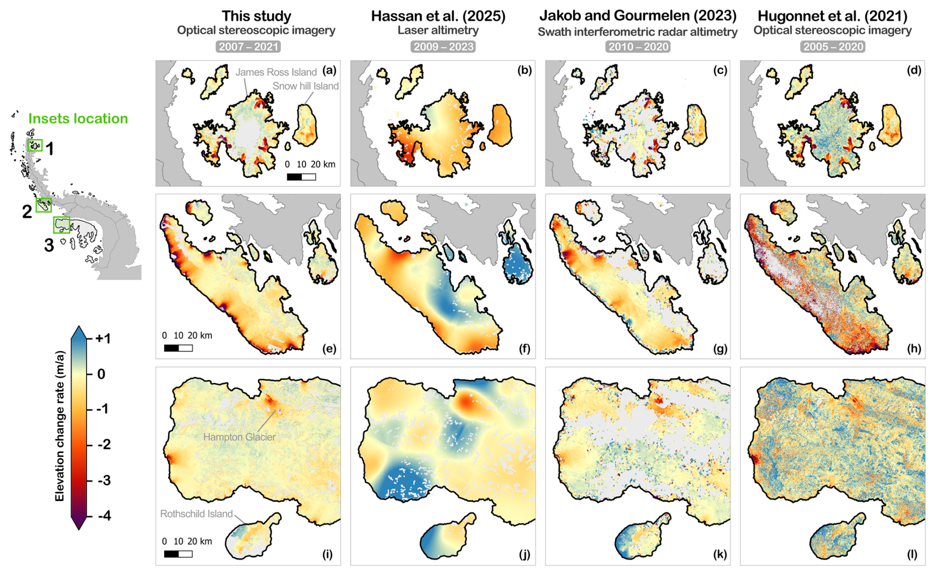
Figure 9 Spatial comparison of elevation change rates maps on selected peripheral glaciers. The results from four different studies (this study, Hassan et al. (2025), Jakob and Gourmelen (2023) and Hugonnet et al. (2021)) are compared over three different sites, on panels (a)–(d) for Vega, James Ross and Snow hill Islands, (e)–(h) for Adelaide Island and (i)–(l) for Alexander Island, respectively. The location of the sites is indicated on the left side. The same color scale is used for all maps and the spatial scale is identical for the three sites. The outlines from RGI Consortium (2023) are plotted in black.

5.1.2 Complementarity between altimetry and optical stereoscopy

The spatial comparison detailed previously also emphasizes the complementarity between the methods, in particular between the laser altimetry and the optical stereoscopic imagery, which both capture surface elevations without firn penetration biases. Satellite laser altimetry measurements, following orbital tracks of variable spacing, require interpolation methods to obtain smooth dh$/\mathrm{d}t$ maps at a spatial resolution of 1–5 km. Over wide homogeneous areas, e.g., the ice sheet areas outside of the northern APIS, this is very suitable and the high vertical accuracy allows one to precisely measure small elevation changes. This is exactly where optical stereoscopic methods can struggle, producing many artifacts, outliers or simply data gaps. However, intense small-scale dh$/\mathrm{d}t$ signals can be missed by sparse laser altimetry measurements. On Fig. 8, the strongly negative dh$/\mathrm{d}t$ signal from Sjoegren and Boydell Glaciers is present in the three high-resolution datasets (this study, 30 m; Seehaus et al. (2023), 30 m, Scambos et al. (2014), 50 m), but not in the 5 km one (Smith et al., 2020). Likewise, the localized thinning of Crane, Flask and Leppard Glaciers is completely absent from this dataset. Additionally, when the signal is sufficiently wide to be observed by laser altimetry, the elevation change measurements are still lower (in absolute value) than those observed by high-resolution methods. For example, the HGE glacier system elevation change signal is less negative and more spread out on Fig. 8b than on the other panels a, c and d. Furthermore, the laser altimetry can be very sensitive to outliers that sometimes propagate, as around the Getman Ice Piedmont Glacier (Fig. 8g) or on Alexander Island (Fig.  9j). On the other side, optical stereoscopy allows the observation of very local changes at high spatial resolution. Still, it requires costly data processing and storage, and remains less efficient than laser altimetry on homogeneous areas, in terms of data gaps and vertical accuracy. This illustrates the potential of combining optical stereoscopic dh$/\mathrm{d}t$ maps and laser altimetry to observe ice sheet and glacier elevation change at small scale as well as over wide homogeneous areas.

5.2 Mass changes of the AP

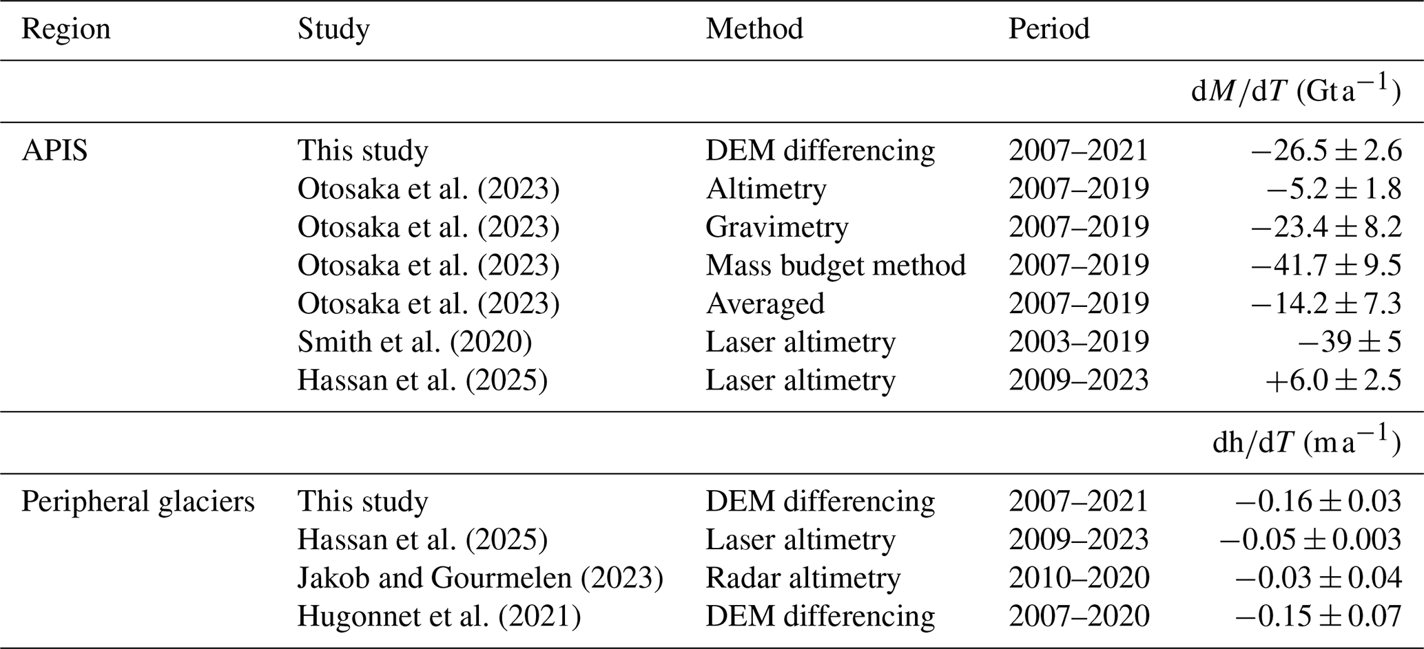
We extracted the APIS mass changes for the three ice sheet observation methods from the Otosaka et al. (2023) aggregated time series, as well as the averaged estimate (Table 2). We selected the closest period available (2007–2019) to the one of this study (2007–2021). Our mass change estimate (−26.9 ± 5.3 Gt a⁻¹) falls within the methods' spread, but is notably more negative than the averaged estimate of −14.2 ± 7.3 Gt a⁻¹. In particular, it is close to the gravimetry estimate (−23.4 ± 8.2 Gt a⁻¹). Still, our mass change estimate for the peripheral glaciers (−13.8 ± 1.4 Gt a⁻¹) is four times more negative than the one used in Otosaka et al. (2023) to correct the gravimetry estimate (less than 3 Gt a⁻¹). This underlines that correcting for peripheral glacier mass changes is not an easy and straightforward task, and should not be neglected. This also implies that agreement with gravimetry may be coincidental. The mass budget method gives a much more negative mass change (−41.7 ± 9.5 Gt a⁻¹) whereas the altimetry provides closer to zero figures (−5.2 ± 1.8 Gt a⁻¹). Seehaus et al. (2023) also reported more negative mass change rates than those provided by the altimetry in a radar DEM study restricted to the northern AP between 2013 and 2017.

The differences between the altimetry estimates and the estimates based on DEM analysis, though both belong to the same elevation-differencing group of methods, can be attributed to a variety of sources. Altimetry studies tend to provide generally less negative mass change estimates (e.g. Schröder et al., 2019, Hassan et al., 2025), except for Smith et al. (2020), who obtained a mass change of −39 ± 5 Gt a⁻¹ over the period 2003–2019. Despite using similar laser altimetry data over close time periods, Hassan et al. (2025) report substantially different results from Smith et al. (2020), which highlights the influence of data processing and elevation corrections. Discrepancies between elevation change maps derived from altimetry and from DEMs differencing highly depend on the area considered. When comparing the map from Smith et al. (2020) to the results from our study (Fig.  S12), the mean elevation change rate difference is negligible over the ZWA12 southern regions 24 and 27 (0.002 and 0.008 m a⁻¹ respectively). Those two regions are the largest of the AP and present a gentle topography that is accurately captured by laser altimetry. However, the elevation change rate difference is much larger over northern regions 25 and 26, reaching −0.10 and −0.14 m a⁻¹ respectively. Two distinct spatial patterns explain these discrepancies. First, interpolation errors in laser altimetry propagate outliers, which are more likely to remain due to the complex topography. For example, a small part of the northern tip of the Trinity Peninsula alone accounts for an unrealistic mass change of 10 Gt a⁻¹ in Smith et al. (2020)'s study. Second, the limited spatial resolution generates a bimodal pattern observed on many intensely thinning glaciers, such as Hektoria, Drygalski and Fleming Glaciers. The most negative dh$/\mathrm{d}t$ values at low elevations (0–700 m) are overestimated, i.e. too positive, and the less negative dh$/\mathrm{d}t$ values at medium elevations (above 700 m) are underestimated, i.e. too negative, because of signal leakage. This systematically induces an overestimation of mean elevation change rates, up to 1.05 m a⁻¹ (Crane Glacier) and 2.17 m a⁻¹ (Hektoria Glacier) from the laser altimetry maps. Thus, if an apparent agreement can exist between laser altimetry and DEM differencing at AP scale, it is most likely coincidental and conceals significant spatial differences related to the methods' limits.

Next, we compared the elevation changes obtained over the peripheral glaciers to the three studies mentioned in Fig. 9. The two global studies (Jakob and Gourmelen, 2023 and Hugonnet et al., 2021) do not apply any FAC correction, using instead a constant density conversion factor to get mass changes. Therefore, we directly compared the elevation changes of all four studies (and not the mass changes). We obtained more negative elevation change rates compared to the two altimetry studies, which is consistent with the tendency of altimetry to produce less negative estimates over the APIS (except for Smith et al. (2020)). Despite the high level of noise coming from the ASTER sensor, the maps from Hugonnet et al. (2021) integrated over the peripheral glaciers produce very similar results to our study. This suggests that observations by DEM differencing are reliably repeatable despite the use of different sensors.

Otosaka et al. (2023)Otosaka et al. (2023)Otosaka et al. (2023)Otosaka et al. (2023)Smith et al. (2020)Hassan et al. (2025)Hassan et al. (2025)Jakob and Gourmelen (2023)Hugonnet et al. (2021)

Table 2 Comparison of mass changes over the APIS and elevation changes over the peripheral glaciers. For each study, the method and period selected are indicated. We compare mass change rates over the APIS and elevation change rates over the peripheral glaciers.

5.3 Focus on prominent areas

5.3.1 Larsen B embayment

The Larsen B embayment is located on the northeast coast of the AP. It hosted the Larsen B Ice Shelf that was fed by several tributary glaciers until the ice shelf broke up in 2002. This event triggered an intense thinning and acceleration of all tributary glaciers (e.g. Hektoria, Green, Evans, Crane) and has been widely analyzed (e.g. Scambos et al., 2004; Rott et al., 2018). Only a portion of the ice shelf remains, known as the Larsen B remnant or SCAR Inlet Ice Shelf, providing a temporary buttress to Leppard and Flask Glaciers in particular. Other studies have worked on understanding the complex dynamics of the Larsen B Embayment glaciers, showing phases of retreat and re-advance (e.g. Ochwat et al., 2025, Surawy-Stepney et al., 2024, Fluegel and Walker, 2024). The Larsen B Embayment has been repeatedly identified as the most intensely thinning area of the APIS over the past two decades (e.g. Seehaus et al., 2023, Scambos et al., 2014), and we confirm this. On Hektoria Glacier, the most negative dh${}_{\mathrm{ice}}/\mathrm{d}t$ rates are found between 6 and 16 km upstream from the 2011 glacier's front (before the 2011–2022 readvancement, Fluegel and Walker, 2024), reaching −17.1 m_ice a⁻¹. The same pattern is observed on Green, Evans and Crane Glaciers, where elevation change rates peak a few kilometers away from the glacier front at −13.8 m_ice a⁻¹, −6.7 m_ice a⁻¹ and −5.2 m_ice a⁻¹ respectively. Leppard and Flask are still buttressed by the SCAR Inlet Ice Shelf, and show less negative dh${}_{\mathrm{ice}}/\mathrm{d}t$ signals (−3.2 m_ice a⁻¹ and −2.7 m_ice a⁻¹ at minimum). However, the gradual decline in stress caused by the increasing instability of the ice shelf over the period could explain the observed thinning pattern of these two glaciers (Li et al., 2021). Even though the Larsen B tributary glaciers represent only 2 % of the AP area, they contribute significantly to the total AP mass losses. Over 2007–2021, Hektoria Glacier (−2.3 ± 0.2 Gt a⁻¹) and Green Glacier (−1.80 ± 0.1 Gt a⁻¹) are listed among the 30 highest contributors. More generally, the Larsen B tributary glaciers present a total mass change rate of −6.92 ± 0.7 Gt a⁻¹, corresponding to 17 % of AP mass loss. While those mass changes are in continuity with the 2002–2011 estimate of −8.9 Gt a⁻¹ from Berthier et al. (2012), the region has by then undergone several major changes as a result of short-term climate trends (e.g. Ochwat et al., 2024) that cannot be disentangled in our analysis.

5.3.2 Fleming Glacier

Fleming is a large glacier located on the southwest coast of the AP, historically feeding an ice shelf in Wordie Bay along with other smaller tributary glaciers (Rotz, Airy, Seller and Prospect). The dynamic evolution of Fleming and its neighbor glaciers after the slow disintegration of the ice shelf between 1960 and the late 1990s has been documented by several studies, in terms of velocity, elevation or grounding line changes. Zhao et al. (2017) reported a decrease of dh$/\mathrm{d}t$ comparing the periods 1966–2008 and 2008–2015 over Fleming Glacier. They found elevation change rates of −1.5 m a⁻¹ at the front of the glacier between 1966 and 2008 and minimum elevation change rates of −1.9 m a⁻¹, reached in areas more upstream. Looking at the period 2007–2021, we also obtained elevation change rates much more negative than the Zhao et al.'s first period (1966–2008), −2.7 m a⁻¹ at the glacier front and −6.5 m a⁻¹ at minimum, corroborating the intensified thinning of Fleming glacier over the past decades. The most negative elevation change rates are located a few kilometers upstream from the glaciers' front, closer to the front than reported by Friedl et al. (2018) over 2011–2014. Our study also shows that Airy glacier presented less negative elevation change rates in comparison to the other glaciers, likely related to a more favorable bedrock geometry. The Fleming catchment, encompassing Fleming, Rotz, Airy, Seller and Prospect glaciers in SIL20 outlines, presented a mass change rate of −5.3 ± 0.2 Gt a⁻¹, second largest contribution in ice mass loss over the period 2007–2021. These significant figures suggest that the tributary glaciers of the former Wordie Bay ice shelf are still responding dynamically to its breakup, and that they have not yet found a new equilibrium state by 2021.

5.3.3 Tidewater glaciers of the northwest AP

Tidewater glaciers of the northwest AP have presented different dynamic behaviors over the past few decades, which have been predominantly linked to an oceanic forcing. Cook et al. (2016) identified two different oceanic circulations controlling the position of glacier's front over multidecadal time scales. In the northern part of the AP's west coast, glaciers are exposed to the cool Bransfield Strait Water (BSW). Further south, from Anvers Island until the north of Alexander Island, the oceanic circulation is dominated by the warm Circumpolar Deep Water (CDW). The CDW presents a particular depth pattern: a cooling trend is observed up to 100 m depth, followed by a warming trend below 200 m depth and beyond. According to Cook et al. (2016), this warming is a primary control of the retreat observed for many glacier's front exposed to the CDW.

Investigating the consequences of the subsurface ocean warming, Wallis et al. (2023) documented the evolution of Cadman Glacier over the past three decades. Following a period of front stability until the early 2000s, the glacier started to retreat at a moderate rate. It underwent an intense acceleration event in 2018–2019, which was related to the long-term thinning of its ice shelf. In March 2021, the latter collapsed entirely, leading to a 5.2 km-front retreat and contributing to the glacier's acceleration and thinning. Wallis et al. (2023) report extreme elevation change rates of −20.1 ± 2.6 m a⁻¹ after the 2019 acceleration, which is indeed more negative than our rate of −10 m a⁻¹ over the period 2007–2021. They highlighted that the dynamic thinning affected inland areas up to 8 km away from the 2015 grounding line. We also identify this propagation of negative elevation rates, but the reported value of −3.0 ± 0.5 m a⁻¹ is reached 6 km closer to the grounding line. Their work suggests that thinning intensified towards the end of our study period, which would explain why we observed less negative elevation changes over the entire 2007–2021 period.

Unlike Cadman Glacier, the Funk and Lever neighboring glaciers have shown constant velocities and stable terminus over the past decades (Wallis et al., 2023). We confirm that between 2007 and 2021, a much more negative elevation change was obtained for Cadman Glacier (−0.89 ± 0.12 m_ice a⁻¹) than for Funk and Lever Glaciers (−0.06 ± 0.08 m_ice a⁻¹ and −0.13 ± 0.10 m_ice a⁻¹, respectively). Moreover, several nearby glaciers presented thickening glacier tongues, including Trooz and Funk Glaciers, which participate in the slightly positive or close-to-zero mean elevation change obtained for these glaciers. Wallis et al. (2023) postulated that the disparities between the recent dynamic evolution of the Cadman Glacier and the neighboring glaciers are related to the different bathymetry configurations. Following this, the seabed dataset provided by Lavoie et al. (2015), based on swath multibeam data sets from five national programs, provides some insight into the elevation changes of several glaciers of the northern AP. Shallow trough bathymetry is often associated with low glacier flux in this area (Davison et al., 2024). For example, the basin in front of Iliad Glacier, presenting a mildly positive elevation change (+0.22 ± 0.12 m_ice a⁻¹), is notably shallow (< 300 m). Similarly, the positive elevation changes observed on other glaciers of Anvers Island could be related to the shallow bathymetry near the island's eastern coast. The area just offshore of the Jason Peninsula is also very shallow, but glaciers at the very tip of the Peninsula tend to present slightly negative elevation changes. The positive elevation changes of the other glaciers of the Jason Peninsula are likely explained by buttressing from SCAR Inlet Ice Shelf.

Along the Trinity Peninsula and the Davis and Danco Coasts, exposed to the BSW, we observe that glaciers have remained stable or even thickened over the period 2007–2021 (Fig. 6), in accordance with the results from Cook et al. (2016) and Davison et al. (2024). Further south along the western coast, between Anvers and Adelaide Island, elevation changes are mostly negative, except for a few glaciers close to equilibrium. Adelaide, Renaud and Lavoisier Islands also host some of the most thinning glaciers, which is consistent with the CDW predominance in the southwestern part of the AP. However, we observe no clear relationship between elevation changes and Bedmap3 bathymetry at glacier's front for catchments exposed to either CDW or BSW (not shown). As the widespread ice discharge increase reported by Davison et al. (2024) started in ∼ 2019, at the very end of our study period (2007–2021), it might require more time to initiate significant negative elevation changes. This increase could also be the result of the thickening of glacier tongues (Fig. 6). Furthermore, the difficulty to constrain bedrock models in many places hinders accurate bathymetry estimates. Large discrepancies appear between the different models (e.g. Shahateet et al., 2023), complicating the identification of significant correlations. More broadly, the relationship between elevation changes and bathymetry at the glacier's front is likely to be more complex than simply depth-dependent. Taking other parameters into account, such as the bed geometry and inclination, could be beneficial to better understand the spatial variability of elevation changes over the northwestern AP.

5.4 Strengths, limitations and perspectives

5.4.1 Elevation corrections

The choice of a GIA or elastic rebound model has minor implications for the final volume changes. The associated corrections systematically represent less than 4 % of the signal, and fall within the observational uncertainty. However, the crustal deformation corrections applied in the study (GIA and ELR) do not account for recent viscoelastic response, which might be required to fit with observed bedrock uplift rates (Nield et al., 2014; Samrat et al., 2020). The misfit induced could exceed the GIA and ELR signals in the northern Peninsula. Even if the signal amplitude remains lower than the firn-related uncertainty in this region (Fig. S6), future studies should consider applying a viscoelastic correction at the AP scale in order to account more accurately for crustal deformation.

On the other hand, the four FDMs used in this study lead to significantly different estimates, both in terms of spatial patterns and numerical values. To get a sense of the FAC correction applied, we calculated the mean density corresponding to the volume changes observed. We obtained a density of 878 ± 62 kg m⁻³ (1σ spread between the models) for the APIS and 843 ± 50 kg m⁻³ for the peripheral glaciers. This number falls into the uncertainty bar of the density conversion factor commonly used by the glacier and ice cap community, 850 ± 60 kg m⁻³ from Huss (2013). However, at the AP scale, the FAC correction induces the largest uncertainty (Fig. S13). It accounts for up to 20 % of the signal on some glaciers, with a large spread between the models over the AP, reaching 0.08 m a⁻¹ at maximum. Given the 14-year study period, which allows for limited densification and therefore limits the impact of the model densification choices, the likely sources of differences in FAC change are the forcing (as described in Mottram et al., 2021), surface parameterizations (e.g. surface snow density), and potentially the treatment of liquid water from melt and rain. The spatial resolution, ranging from 10 km (GEMB-FDM) to 27.5 km (MAR-FDM) may also affect the ability of the models to resolve small-scale spatial patterns, such as the East-West gradient across the AP. This is particularly visible in the northern AP, where the standard deviation between the models reaches its maximum (Fig. S6). The AP is a difficult place to validate climate and FDM models due to the scarcity of in situ measurements. The period selected to compute the FAC correction (start, end or entire summer) also affects the results at orders of magnitude similar to the spread between the models. Thus, the conversion from volume to mass, applied through the FAC correction, constitutes one of the major limitations of this method. A better understanding of firn processes and firn modeling is therefore a priority to improve the DEM-differencing method for glaciers and ice sheets mass changes studies (The Firn Symposium team et al., 2024).

5.4.2 Interpolation

As a third of AP area is not covered by observation data, interpolated data represent a non-negligible part of the final estimates. Over large regions of the APIS, the interpolation represents the second source of uncertainty (Fig. S13). For example, the mass changes obtained for Region 24 using the ZWA12 outlines (−8.0 ± 3.4 Gt a⁻¹, Fig. 7a) includes a large uncertainty that is essentially caused by the partial coverage of dh$/\mathrm{d}t$ maps (57 %). The local hypsometric interpolation performs well in smooth high altitude areas but struggles more reproducing local patterns of intense thinning at lower elevations (e.g. Drygalski or Fleming Glaciers). If some of the contrasting dh $/$ dh spatial patterns do come from observations (e.g. Stefan Ice Piedmont and Peter Glaciers, Cadman Glacier, Fig. 7), the interpolation can artificially generate contrasted values, as in the south of Anvers Island (Fig. 7). Glaciers' mean ice elevation changes must therefore be interpreted with caution, especially when dh$/\mathrm{d}t$ observations are scarce. We suggest the interpolation could be improved by taking into account more input data to explain the spatial variability of the dh$/\mathrm{d}t$ signal (e.g. velocity acceleration). As mentioned in Sect. 5.1.2, another alternative to fill data gaps could be to combine laser altimetry maps, which may allow to better reproduce the spatial patterns.

5.4.3 Grounding line

The grounding line is a physical delimitation difficult to observe, both with in situ and satellite measurements (Friedl et al., 2020). Its location depends on many poorly constrained factors, including bedrock geometry and ice thickness. AP-scale grounding line datasets are scarce and not available at an annual resolution. Nevertheless, rapid fluctuations, including frequent retreat of the grounding line, are induced by glacier dynamics at sub-annual scales. In many areas, the position of the grounding line has not yet been agreed upon (e.g. Hektoria Glacier, Ochwat et al., 2025). Here, considering a 14-year period complicates the choice of grounding line dataset. The grounding line from the first epoch may encompass areas that subsequently became ungrounded, while the one from the second epoch could miss former grounded ice changes. Cadman Glacier illustrates this dilemma, exhibiting pronounced differences between the grounding line datasets used in this study. However, we emphasize that a limited number of AP's glaciers are prone to those grounding line disparities. With the SIL20 outline, Cadman Glacier (Fig. 6) presented mass changes of −0.27 ± 0.02 Gt a⁻¹ over a total area of 332 km². The Bedmap 3 grounding line (Pritchard et al., 2025), located ∼ 5 km more inland, identifies the lowest portion of the glacier as the ice shelf. This area, covering 15 km², lost 0.03 Gt a⁻¹, which represents ∼ 10 % of the SIL20 outlines estimate. At the scale of the AP, the mass changes caused by grounding line differences are negligible. Nevertheless, catchment-scale studies might require a more accurate grounding line, including knowledge of its migration.

5.4.4 Time constraints

As each epoch extends over three years, we cannot exclude potential influence of inter annual variations that affect the mass change results, such as the strongly positive surface mass balance in 2022 (Wang et al., 2023). Still, we tried to reduce the seasonal influence by establishing strict constraints on the seasonal time difference between the acquisitions. Our elevation change maps are based on the comparison of DEMs over two epochs and hence does not allow us to observe and analyze elevation changes throughout the period. For example, potential variations of the elevation difference rates trends or specific events happening during the time period cannot be isolated in this study. This is quite clear when comparing the results from Scambos et al. (2014) and Seehaus et al. (2023), that cover two distinct time periods and show contrasted elevation changes over the fast-changing glaciers. The extreme changes that Hektoria Glacier underwent over the two past decades (slow retreat between 2002 and 2011, followed by a readvancement until the 1.5-year extreme retreat starting in 2022, Fluegel and Walker, 2024 and Ochwat et al., 2025) cannot be identified either. This is also the case for many other physical processes presenting a strong inter annual variability (e.g. summer melt, Barrand et al., 2013). However, a key advantage of our large study period is that it greatly reduces the noise, especially at high elevations.

6 Conclusions

By combining DEMs derived from stereoscopic images with accurate laser altimetry data, we mapped elevation changes over the Antarctic Peninsula from 2007 to 2021 with substantially improved accuracy and spatial resolution relative to previous studies. Our dataset provides an unprecedented overview of AP glacier mass changes, at regional and local scales, encompassing both the ice sheet and the peripheral glaciers. Taking into account changes in firn air content and crustal rebound processes, we obtained a total mass change of −41.9 ±8.5 Gt a⁻¹ over the Antarctic Peninsula (two thirds from the ice sheet and one third from peripheral glaciers), equivalent to a sea-level contribution of 0.12 ± 0.02 mm a⁻¹ (3 % of the 2007–2021 sea-level rise). The rate of elevation change for peripheral glaciers (−0.16 ± 0.03 m_ice a⁻¹) is slightly more negative than over the ice sheet (−0.11 ± 0.01 m_ice a⁻¹). We report contrasting regional mass changes, ranging from moderate mass gain in the southeast of the AP to considerable mass losses in all other regions. Investigating the oceanic forcing in the northwestern portion of the AP and the bathymetric correlation of mass losses, we do not find a clear relationship, despite a strong latitudinal pattern of mass changes. However, the elevation change rate maps reveal changes in glaciers that have not received much attention yet, even though they also show striking thinning patterns, such as on Liard Island or the smaller glaciers in Wordie Bay. By reaffirming the importance of regional-scale studies, we also point out the underlying need for an exhaustive list of glacier names and outlines that can be used in consensus by the community. Ultimately, this study also underscores the important role of projects such as SPIRIT and REMA in collecting consistent region-wide datasets, which are essential for gaining a coherent perspective on glacier changes. The continuity of such observations should be a priority of space agencies.