Estimation of snow depth from AMSR-2 based on an AutoML method over the Qinghai-Tibet Plateau

Snow depth is a crucial parameter for describing the spatiotemporal variations of snow cover, and passive microwave snow depth products (10–25 km) are widely used for monitoring snow depth changes. However, as one of the three major snow-covered regions in China, the Qinghai-Tibet Plateau has complex terrain and rapid changes in snow cover with strong spatial heterogeneity, making it difficult for coarse-resolution snow depth products to accurately describe its spatiotemporal characteristics. This study proposes a high spatial resolution (500 m) snow depth estimation method based on the Advanced Microwave Scanning Radiometer 2 (AMSR-2) brightness temperature data and Automated Machine Learning. Firstly, using Pearson correlation coefficients, 19 key factors influencing snow depth, including AMSR-2 brightness temperature, slope, and surface roughness, were selected as input data (independent variables) for Automated Machine Learning. Meanwhile, passive microwave downscaled snow depth data and ground-based snow depth measurements were introduced as dependent variables for Automated Machine Learning. The Automated Machine Learning model was then trained separately for four different types of snow cover surfaces (forest, grassland, water, and bare land). Finally, through ten-fold cross-validation, the optimal machine learning model for snow depth estimation under each type of underlying surface coverage was selected, thus generating sequential snow depth datasets for the ten-year snow cover period of the Qinghai-Tibet Plateau from 2012 to 2021. Results show that (1) the estimated snow depth values well with ground-based observations, yielding a coefficient of determination (R²) of 0.71 and a root mean square error (RMSE) of 3.64 cm, indicating high estimation accuracy. (2) Snow depth estimation demonstrates the highest accuracy in unused land (CatBoost, R²=0.82), followed by grassland (CatBoost, R²=0.77, RMSE=3.11 cm), water (ET, R²=0.75, RMSE=2.20 cm), and forest (XGBoost, R²=0.71, RMSE=3.30 cm). (3) A comparison with snow cover extent derived from Landsat-8 optical imagery reveals that the estimated snow depth spatial distribution is consistent with snow cover extent, providing reliable data for monitoring snow cover changes in mountainous regions.

1 Introduction

Snow cover is a crucial component of the cryosphere, playing a vital role in global ecosystems, hydrological cycles, and human societies. Snow depth (SD) is an essential attribute that describes the spatiotemporal variation of snow cover, and it serves as a key parameter in various domains, including climate change and the hydrological cycle. The Qinghai-Tibet Plateau (QTP), often referred to as the “Roof of the World” is one of the three major snow-covered regions in China and a sensitive area for global climate change (Tedesco et al., 2010; Zhang et al., 2008). As global temperatures rise, the QTP has experienced significant temperature changes, accompanied by a reduction in snow cover over the years, characterized by highly uneven spatial distribution. Since the 2000s, SD on the QTP has shown a clear downward trend, with notable differences in its spatiotemporal distribution patterns (Che et al., 2019; Wang et al., 2022; Bo et al., 2014). Therefore, monitoring SD changes on the QTP is of great importance for meteorological forecasting, water resource management, hydrological modeling, and other related fields.

Research on SD retrieval using passive microwave (PMW) remote sensing has been conducted for more than four decades, leading to the development of multiple mature inversion algorithms and the release of various SD products. At present, PMW-based SD inversion methods can be broadly classified into four categories: physical model–based methods, data assimilation approaches, semi-empirical statistical methods, and machine learning (ML) techniques. Physical model based methods simulate microwave scattering and absorption processes within the snowpack by explicitly considering snow properties such as density and grain size. However, the complexity of microwave radiative transfer modeling and the difficulty of accurately obtaining snow physical parameters often reduce the reliability of these approaches (Kwon et al., 2017; Wainwright et al., 2017). Data assimilation methods improve SD estimation accuracy by optimally integrating PMW observations with auxiliary information prior to model flux estimation, yet their performance is highly dependent on the quality and availability of observational data (Cortés and Margulis, 2017; Aalstad et al., 2018). Over the QTP, the scarcity of in situ observations considerably constrains the applicability of data assimilation–based SD retrieval (Li et al., 2022b).

Semi-empirical statistical methods primarily exploit the relationship between SD and the difference in snow scattering characteristics observed at different PMW frequencies. Among these, the brightness temperature (BT) gradient method proposed by Chang et al. (1987) has been widely adopted, and numerous studies have subsequently improved upon the original Chang algorithm (Cao et al., 1993; Che et al., 2008; Foster et al., 1997; Jiang et al., 2014; Kelly, 2009). Che et al. (2008) modified the Chang algorithm using SD observations from Chinese meteorological stations to account for the relatively low snow density in China, resulting in the release of two long-term SD datasets, namely the Che_SSMI/S and Che_AMSR2 products. In addition, several studies have developed SD inversion algorithms tailored to specific underlying surface types (Derksen et al., 2005; Goita et al., 2003; Jiang et al., 2014). For example, Derksen et al. (2005) proposed an algorithm for major land cover types in forested regions of Canada and subsequently estimated SD over mixed pixels. Similarly, Jiang et al. (2014) established a semi-empirical SD inversion algorithm by combining BT data from four frequencies (10, 18, 36, and 89 GHz) and considering four underlying surface types: grassland, farmland, bare land, and forest. Despite their extensive application, semi-empirical statistical methods exhibit notable limitations in mountainous regions. First, the relationship between BT and SD is inherently nonlinear, whereas semi-empirical methods commonly assume a linear relationship, leading to considerable estimation errors (Tanniru and Ramsankaran, 2023). Second, the coarse spatial resolution (approximately 10–25 km) of PMW derived SD products significantly restricts their accuracy in areas with complex terrain (Yan et al., 2022; Tanniru and Ramsankaran, 2023). These limitations hinder the reliable application of semi-empirical SD products over mountainous regions such as the QTP.

In recent years, ML techniques have been increasingly employed for SD inversion. By training models such as Support Vector Machines (SVM), Random Forests (RF), and Artificial Neural Networks (ANN), ML approaches can capture nonlinear relationships between PMW BT and SD, thereby improving retrieval accuracy through the integration of multisource remote sensing data (Xiao et al., 2018; Zhong et al., 2021). Yang et al. (2020) developed an RF based SD retrieval algorithm incorporating BT at multiple frequencies, geographic information, and land cover types, achieving higher accuracy than the Che_SSMI/S and Che_AMSR2 products. Hu et al. (2021) compared ANN, SVM, and RF using multiple SD products and in situ observations as training data and reported that RF exhibited the best overall performance. Moreover, ML methods have demonstrated strong potential for enhancing the spatial resolution of PMW derived SD products. Although ML-based approaches have improved SD retrieval accuracy, several challenges remain unresolved, particularly in complex mountainous regions. Most existing studies rely on a limited number of manually selected ML models, empirical feature selection strategies, and trial and error hyperparameter tuning. Such practices introduce substantial human-induced bias and often result in overfitting, especially under conditions of sparse and unevenly distributed observations, as is the case over the QTP (Du et al., 2020). Consequently, model performance is frequently optimized for specific regions or datasets, while robustness and generalizability across heterogeneous mountainous environments remain limited (Feurer et al., 2015; Hernandez et al., 2025). These issues indicate that the primary challenge lies not only in model performance, but also in the lack of a systematic and objective framework for model selection and optimization in SD inversion.

Automated Machine Learning (AutoML) has emerged as an effective solution to address these methodological by autonomously executing data preprocessing, feature evaluation, model selection, and hyperparameter optimization without extensive human intervention (Ribeiro et al., 2023; Hernandez et al., 2025). The fundamental design philosophy of AutoML is to reduce human bias and enhance the robustness, stability, and reproducibility of ML models (Benghzial et al., 2023). Auto-WEKA, proposed by Thornton et al. (2012), represents one of the earliest AutoML frameworks (Kotthoff et al., 2017), and has since been followed by the development of various AutoML platforms, including Auto-Sklearn, TPOT, H2O, and PyCaret (Feurer et al., 2015; LeDell and Poirier, 2020; Olson and Moore, 2016). Among these, PyCaret offers a concise and user-friendly interface that enables comprehensive comparison of multiple ML models and ensemble based prediction, thereby improving overall model performance and robustness. Despite its potential advantages, the application of AutoML to SD inversion remains limited, particularly in mountainous regions. A major constraint in applying AutoML-based SD retrieval lies in the requirement for sufficient and reliable training samples. Existing SD products are generally characterized by coarse spatial resolution, while ground-based SD observations over the QTP are sparse and unevenly distributed, with approximately 70 % of stations concentrated in the eastern region. These data limitations pose significant challenges for model training and validation in complex terrain.

To address the key challenges of SD inversion in sparsely observed regions, especially those with complex mountainous terrain, this study proposes a more accurate and robust SD retrieval method. The core innovation lies in the integration of multisource data, including downscaled SD data and ground-based measurements, into the PyCaret AutoML framework. This approach not only improves SD retrieval accuracy but also overcomes the limitations of existing methods that struggle with data scarcity and terrain complexity. Moreover, the automatic model selection feature of PyCaret helps mitigate human bias in model choice, ensuring the robustness and generalizability of the results. The findings provide reference for improving SD estimation techniques, particularly in cold regions with complex topography. The remainder of the paper is organized as follows: Sections 2 and 3 introduces the study region, data and methods; Sect. 4 describes the results; Sects. 5 and 6 present the discussion and conclusions.

2 Study area and data

2.1 Study area

The QTP, located in the southwestern region of China, is often referred to as the “Roof of the World” and the “Water Tower of Asia” (Pu and Xu, 2009). As depicted in Fig. 1, the QTP features a highly complex and fragmented terrain, with a general gradient from high in the northwest to low in the southeast, resulting in significant spatial heterogeneity of snow cover (Huang et al., 2019; Ke and Li, 1998; Li et al., 2022b). Furthermore, snow cover on the QTP exhibits distinct seasonal variation, with the widest extent occurring during winter, followed by a gradual decrease in spring and autumn, and the smallest coverage in summer. The snow cover period typically spans from October to March of the following year, with October to December representing the accumulation period, January to February marking the stable period, and March being the melting period (Lu et al., 2008; Ma and Qin, 2012).

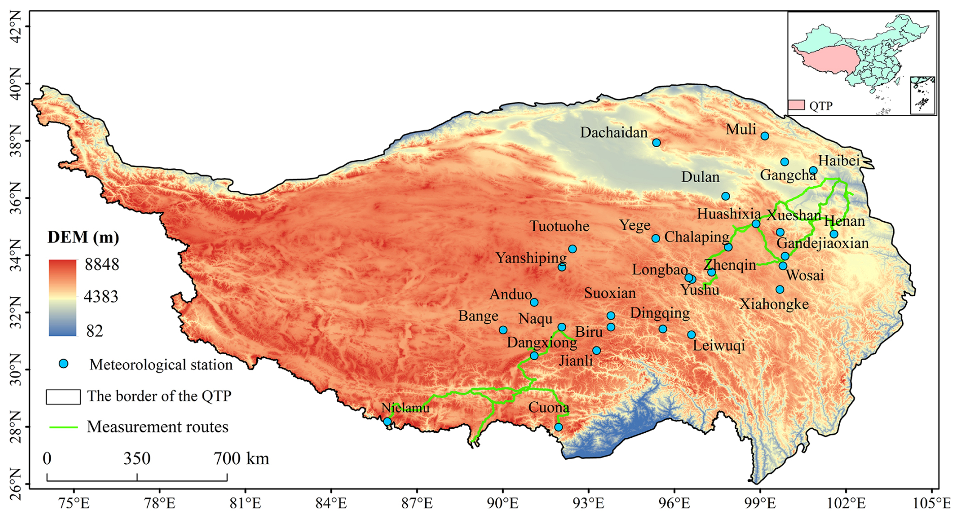
Figure 1 Location of study area and ground-based SD observations.

2.2 Data Sources and Preprocessing

As outlined in Table 1, the dataset used in this study consists of five primary categories: AMSR-2 (Advanced Microwave Scanning Radiometer 2) BT; downscaled SD data (Che_AMSR2_NSD); daily cloud-free snow cover products; ground-based SD observations; and various auxiliary data. All datasets were projected onto the Universal Transverse Mercator (UTM) Zone 45 and resampled to a uniform spatial resolution of 500 m.

Table 1 Basic Information of the Experimental Dataset.

2.2.1 AMSR-2 BT

AMSR-2 is a microwave sensor mounted on the GCOM-W1 satellite, launched by the Japan Aerospace Exploration Agency (JAXA) (Imaoka et al., 2012). It operates across seven frequencies, with each frequency supporting both horizontal and vertical polarization modes (Imaoka et al., 2012). The sensor has a spatial resolution of 10 km and revisits the QTP region every two days. Several studies have shown that the quality of descending BT data is significantly superior to that of ascending BT data (Huang et al., 2022). Therefore, in this study, descending AMSR-2 L1B data were downloaded for five frequencies (10.65, 18.7, 23.8, 36.5, and 89.0 GHz), each with both polarization modes, covering the snow cover period over the QTP from 2012 to 2021. The AMSR-2 data were then resampled to a 500 m resolution using nearest neighbor interpolation to extract BT values corresponding to the SD sample points.

2.2.2 Che_AMSR2_NSD

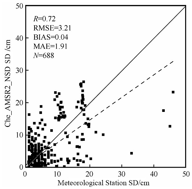
Due to the sparse and uneven distribution of meteorological stations across the QTP, this study used downscaled Che_AMSR2_NSD SD data as the reference dataset. Che_AMSR2_NSD is a 500 m downscaled version of the Che_AMSR2 dataset, derived from a published study that employed empirical fusion rules and snowmelt regression curves (Xu et al., 2024). Compared to ground-based SD measurements, it shows a higher degree of agreement, with a R of 0.72 and a root mean square error (RMSE) of 3.21 cm (Xu et al., 2024). Therefore, Che_AMSR2_NSD, along with ground-based SD observations, was used as a training sample for the AutoML model.

2.2.3 The daily cloud-free snow cover dataset

This dataset is based on long-term MODIS snow cover products, providing daily cloud-free snow cover data at a spatial resolution of 500 m from 2002 to 2024 over the QTP (Huang et al., 2022). Validation results using in situ observations and snow cover data derived from Landsat-8 OLI images indicate that these new snow cover products achieve accuracies of 98.29 % and 91.36 %, respectively (Huang et al., 2018). The dataset is freely available on the Big Earth Data Platform for Three Poles at https://doi.org/10.11888/Cryos.tpdc.272204 (last access: 17 April 2026; Huang and Xu, 2022). In this study, daily snow cover data from 2012 to 2021 were downloaded for the snow cover periods over the QTP to determine the presence or absence of snow in individual pixels. Pixels without snow were assigned a value of 0, while the value for snow-covered pixels was calculated using the algorithm proposed in this study.

2.2.4 SD observations

The ground-based SD observations used in this study were categorized into two types: measurement routes and meteorological stations. The first step in this research involved collecting a comprehensive dataset from the “Survey of Snow Characteristics and Distribution in China” project, which was based on measurement routes and provided a detailed overview of the study area. This dataset includes data from three snow survey routes in China from 2018 to 2019, covering over 200 manually observed snow sample points (Li et al., 2022a). Additionally, meteorological station SD observations were obtained from an automatic measurement dataset for the QTP (2015–2016) (Jiang et al., 2017) and regular stations in typical regions of China during 2017–2019 (Li et al., 2021). These data were sourced from the China Scientific Data and the National Cryosphere Desert Data Center. In this study, SD observations from even-numbered dates were selected as input data for the AutoML model, while data from odd-numbered dates were used to validate the SD estimation results.

2.2.5 Auxiliary Data

The auxiliary data used in this study can be categorized into four main groups: SRTM Digital Elevation Model (DEM), China Multi-period Land Use Remote Sensing Monitoring Dataset, ERA5 Land Temperature Data, and Landsat-8 optical imagery. The SRTM DEM data, generated by the National Aeronautics and Space Administration (NASA) during Earth observation missions, has a spatial resolution of 30 m and is stored in GeoTIFF format. It is freely available from the United States Geological Survey (USGS). Preprocessing steps, including cropping and resampling, were applied to produce a 500 m resolution DEM dataset for the QTP. The China Multi-temporal Land Use Remote Sensing Monitoring Dataset (CNLUCC), derived from Landsat remote sensing images and manually interpreted, has a spatial resolution of 30 m and is available for free download from the Resource and Environmental Science Data Center (Xu et al., 2018). In this study, the classification results from this dataset were used to calculate the proportion of each land cover type in the QTP, identifying major land cover types such as forests, grasslands, water, and unused land. Distinct machine learning (ML) models were then developed to estimate SD for each land cover type. Landsat-8 optical imagery was primarily used for comparative analysis of SD spatial distribution in the Auto_NSD dataset. These images, obtained from the official website of the USGS, have a spatial resolution of 30 m and a revisit period of 16 d. For validation purposes, cloud-free images from seven consecutive days were selected. The ERA5-Land reanalysis dataset, which provides monthly average air temperature data at 2 m above ground level, was also used. Monthly temperature data from the snow season (October 2012 to March 2021) were obtained free of charge from the Copernicus Climate Change Service data platform. These temperature data were then used to analyze the SD results from the AutoML estimation.

3 Methodology

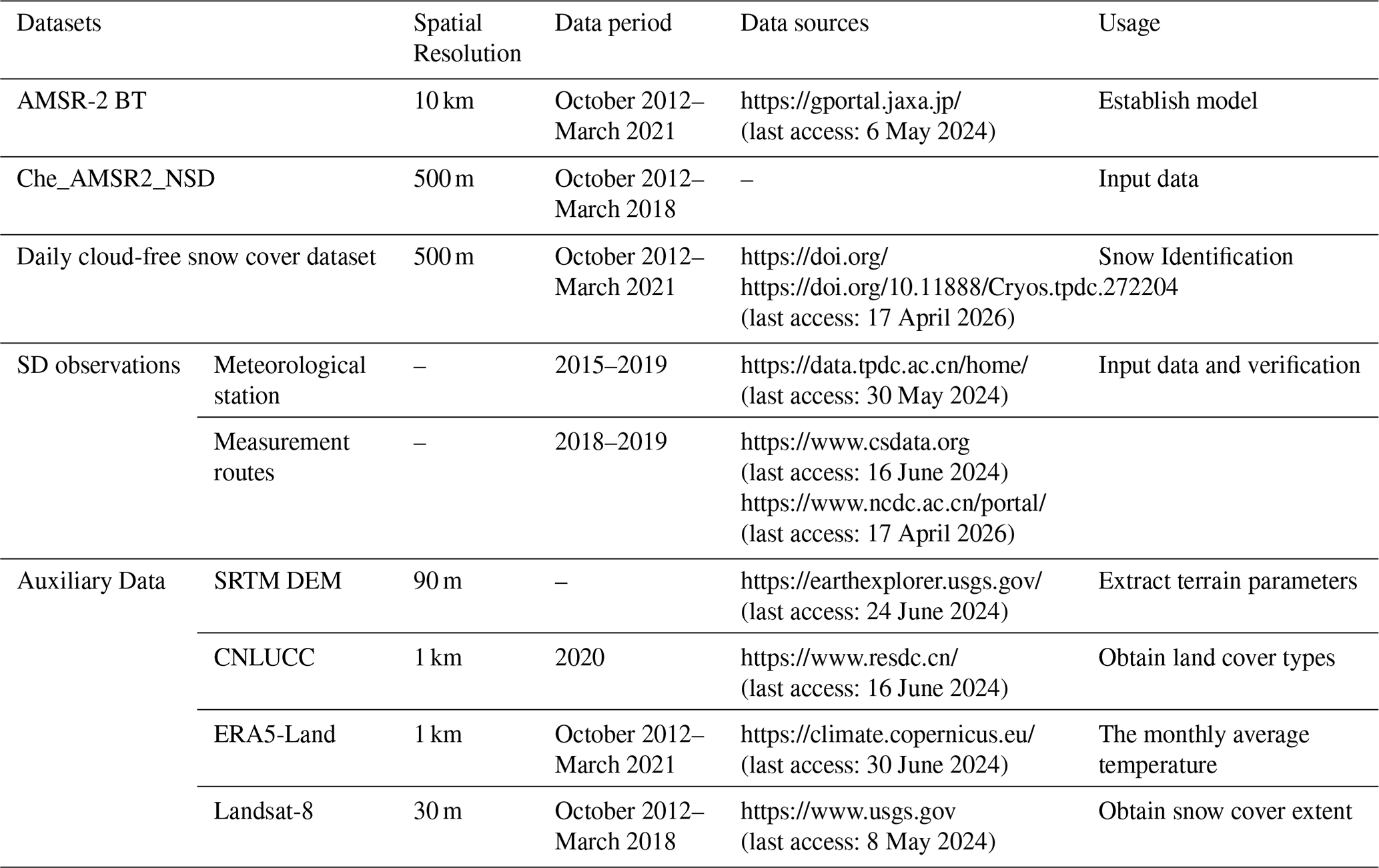
As shown in Fig. 2, the estimation of SD using AMSR-2 BT data and the Pycaret model follows a three-step process. Initially, 19 key factors influencing SD – such as AMSR-2 BT data, slope, and surface roughness – were selected based on the Pearson correlation coefficient method and designated as input variables for the AutoML model. In addition, ground-based SD measurements and 500 m downscaled SD data from a PMW SD product were used as dependent variables for the model. The AutoML model was then trained using the selected input data across four distinct snow underlayment types: forest, grassland, water, and unused land. Subsequently, the optimal ML model for each snow underlayment type was identified through ten-fold cross-validation. Furthermore, the spatiotemporal variation of SD during the snow cover period on the QTP was estimated from 2012 to 2021. The study employed AMSR-2 BT data and influential SD factors, including slope and surface roughness, evaluated through Pearson correlation coefficients, as independent variables. The Che_AMSR2 downscaled SD and ground-based SD observations served as input (dependent) data for the AutoML models, with training conducted under four snow cover types. Finally, the optimal ML model for each land cover type was selected, and SD values were estimated for the QTP snow cover period from 2012 to 2021. The SD for snow-free pixels was assigned a value of 0, while snow-covered pixels were estimated using the proposed method. A detailed technical roadmap for this approach is presented in Fig. 2.

Figure 2 Flowchart of this algorithm.

3.1 AMSR-2 SD estimation based on AutoML

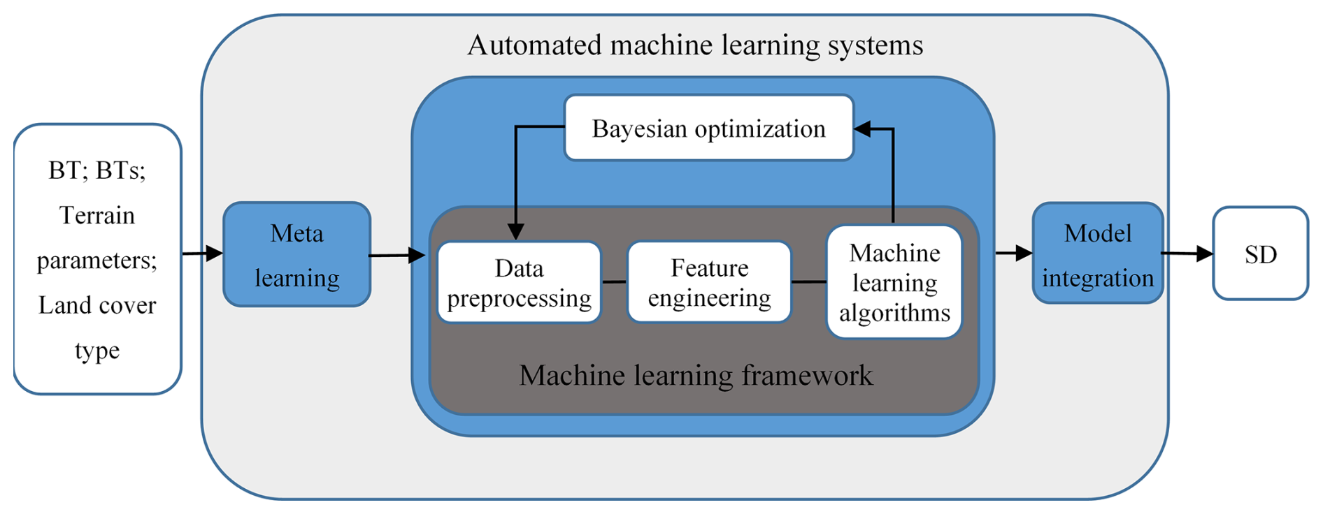
This study utilizes the Pycaret AutoML framework to perform a series of tasks, including data preprocessing and SD model selection. The workflow involves generating multiple models by optimizing the hyperparameters of each model based on user-defined inputs, outputs, and performance metrics (Xu, 2023). The process consists of three main components: meta-learning, Bayesian optimization, and model integration (Fig. 3). In the meta-learning phase, Pycaret continuously refines its learning strategy and model selection by analyzing historical data and model performance, thereby enhancing overall prediction accuracy. Through an in-depth exploration of data features, model algorithms, and hyperparameters, meta-learning enables Pycaret to better understand data complexities and improve prediction outcomes. Bayesian optimization plays a crucial role in calibrating model hyperparameters. By leveraging this technique, Pycaret intelligently selects the next set of hyperparameters based on previous model evaluations, efficiently exploring the parameter space and accelerating the optimization process (da Silva et al., 2025). Lastly, model integration merges multiple high-performing models into a unified entity, thereby improving both the accuracy and stability of predictions.

Figure 3 Flowchart of this algorithm.

The PyCaret framework aims to lower the barriers to entry for machine learning (ML) by providing a more streamlined and efficient workflow, thereby enabling users to more easily compare, select, and deploy ML models. PyCaret integrates three main categories of ML models: generalized linear models, tree-based models, and ensemble learning models. The linear model category includes algorithms such as Ridge regression, Lasso regression, Bayesian Ridge, Lasso Least Angle Regression, and the Huber Regressor. Tree-based models mainly consist of the Decision Tree Regressor, Random Forest Regressor, and Extra Trees Regressor. Ensemble learning models are primarily represented by gradient boosting-based approaches, including Gradient Boosting Regressors, XGBoost, Light Gradient Boosting Machine (LightGBM), and CatBoost regressors (da Silva et al., 2025; Xu, 2023).

3.1.1 Key factor selection

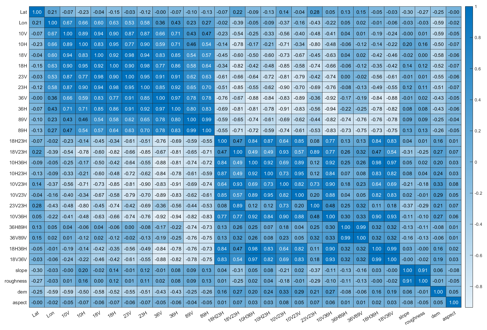
The SD inversion is influenced by several factors, with early research focusing on the sensitivity of various microwave frequencies to snow cover. In this study, SD inversion is performed using the BT values from different microwave frequencies. Chang's algorithm primarily relies on BT data from 18 and 36 GHz to estimate SD. However, in areas with shallow snow cover, the results derived from this algorithm tend to be inaccurate (Chang et al., 1987). Although the 23 GHz frequency is highly sensitive to water vapor in the boundary layer, its sensitivity is comparatively low in terrestrial regions (Liu et al., 2021; Xing et al., 2022). On the other hand, Kelly (2009) found that the 23 GHz channel can effectively identify shallow snow. Additionally, the capacity of different frequency bands to capture snow characteristics varies, and combining these bands provides more comprehensive information about the snow (Liu et al., 2021; Xing et al., 2022). As a result, several studies have used BT data from frequencies such as 89, 23, and 10 GHz for SD inversion (Jiang et al., 2014; Kelly, 2009; Yang et al., 2020a). However, recent research highlights that, in addition to BT values at various frequencies, factors such as geographic location and topographic conditions also significantly impact SD inversion (Huang et al., 2019; Wei et al., 2021). To account for these influences more comprehensively, the present study incorporates BT data from frequencies (10H/V, 18H/V, 23H/V, 36H/V, 89H/V) as well as BT differences (18H23H, 18V23H, 10H36H, 10H23H, 10V23H, 10V23V, 23V23H, 10V36H, 36H89H, 36V89V, 18H36H, 18V36V). Additional geographic parameters, including longitude, latitude, elevation, slope, aspect, and surface roughness, are also considered. This study integrates 28 factors that influence SD. To evaluate the relationships between these variables, the Pearson correlation coefficient (r) was used, calculated according to the following Eq. (1):

$$\begin{array}{}\text{(1)}& r={\displaystyle \frac{{\sum }_{i=\mathrm{1}}^n(\mathit{\text{Xi}}-\stackrel{\mathrm{‾}}{X})(\mathit{\text{Yi}}-\stackrel{\mathrm{‾}}{Y})}{\sqrt{{\sum }_{i=\mathrm{1}}^n(\mathit{\text{Xi}}-\stackrel{\mathrm{‾}}{X}{)}^{\mathrm{2}}}\sqrt{{\sum }_{i=\mathrm{1}}^n(\mathit{\text{Yi}}-\stackrel{\mathrm{‾}}{Y}{)}^{\mathrm{2}}}}}\end{array}$$

Where r represents the Pearson correlation coefficient, Xi and Yi are the samples of the two variables, and $\stackrel{\mathrm{‾}}{X}$ and $\stackrel{\mathrm{‾}}{Y}$ are the mean values of each variable, with n representing the number of samples. The value of r ranges from −1 to 1, where values above 0.90 or below −0.90 indicate a strong positive or negative correlation, respectively.

3.1.2 Model selection and construction

The distribution of meteorological stations across the QTP is sparse, with field-based SD measurements being limited in scope and primarily concentrated in the eastern region. Additionally, the most of meteorological stations is located in grassland or unused land areas. As a result, using only ground-based SD data for AutoML may not adequately represent the entire region. To address this, the study incorporated 471 sample points (Fig. 4) from the Che_AMSR2_NSD dataset alongside ground-based SD observations. When selecting these sample points, factors such as slope direction, elevation, and gradient across different terrains were thoroughly considered to ensure a uniform distribution across the QTP. Moreover, land cover types significantly influence snow accumulation and distribution, which in turn affects the accuracy of SD inversion. This study also explores how mixed pixels impact the precision of SD estimation and develops AutoML models for different land cover types.

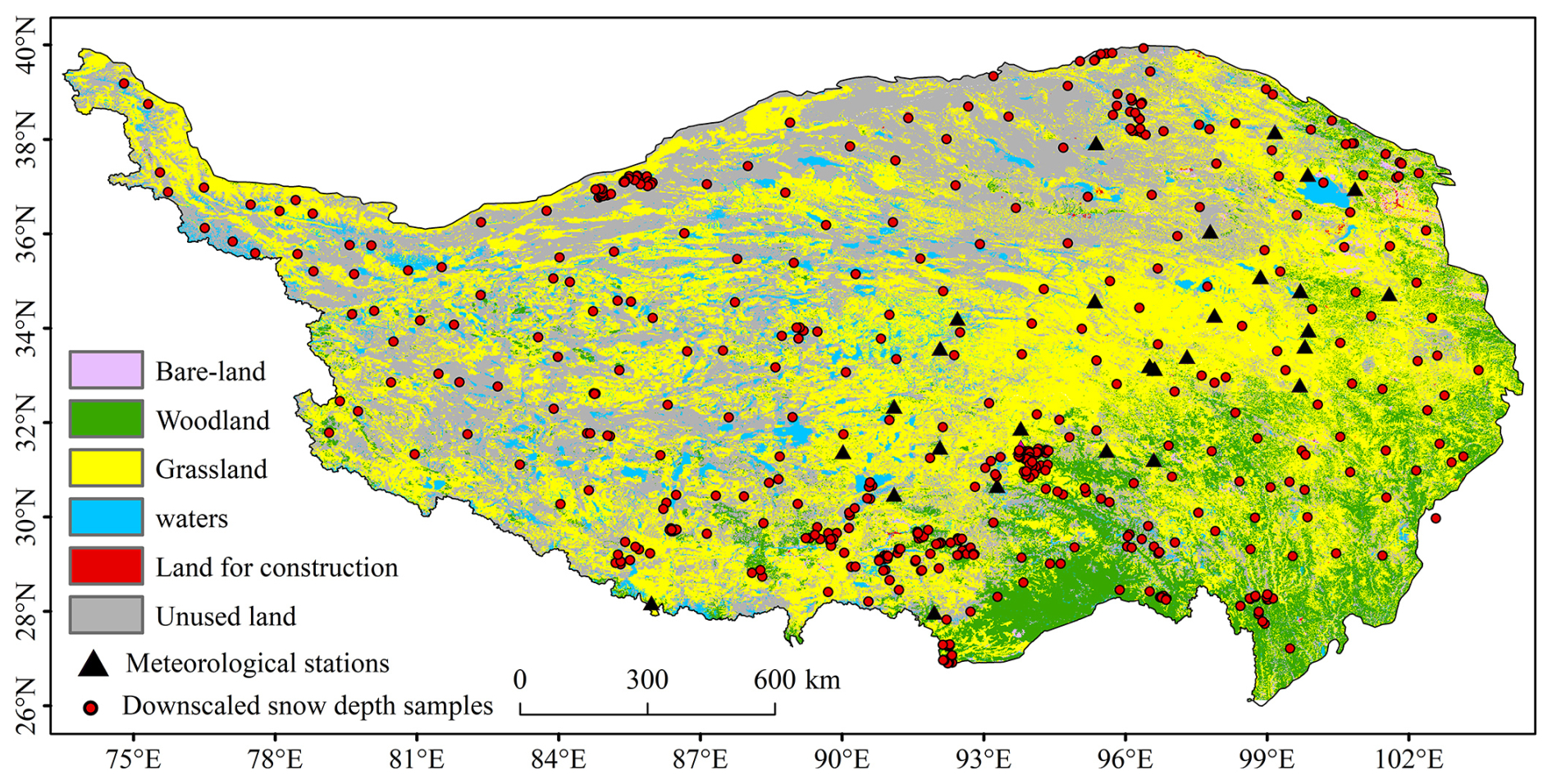
Figure 4 Spatial distribution of input sample data from the AutoML.

In total, 60 forest, 80 water body, 171 grassland, and 160 unused land samples were selected to represent the main land cover types on the QTP. SD data corresponding to each sample point and 19 influencing factors, including BT, BT differences, and topographic features (evaluated using Pearson correlation coefficients), were extracted. Any missing data points were excluded from the analysis. The final dataset included 25 926 forest samples, 340 326 grassland samples, 157 252 water body samples, and 273 672 unused land samples. These samples were processed through the AutoML system, and the random search function was employed to determine the optimal parameters for various algorithms. Accuracy for each ML model, categorized by land cover type, was assessed using ten-fold cross-validation. The model was configured to randomly partition the data into training (90 % of the total samples) and test sets (10 %), with performance evaluated based on the average accuracy from ten iterations. The best-performing ML model was then used to simulate SD across the QTP for the snowpack period from 2012 to 2021.

3.2 Accuracy evaluation method

In this study, the performance of the ML model was evaluated using ten-fold cross-validation, which involves randomly dividing the dataset into 10 equal-sized subsets. In each iteration, one subset is designated as the test dataset, while the remaining nine subsets serve as the training dataset. The model is trained on the training dataset, and its performance is then evaluated on the test dataset. This process is repeated ten times, with each subset being used as the test set once. At the end of the process, the results of all iterations are aggregated, with the mean value typically used as the performance index of the model. This evaluation method assesses the accuracy and reliability of the model. To measure the performance of each ML model, three evaluation metrics were selected: R², RMSE, and MAE.

To quantitatively analyze the SD results estimated by AutoML, four precision evaluation metrics were selected: R², RMSE, BIAS, and MAE. R² and R are used to evaluate the regression model's ability to explain the variation in the dependent variable, with values ranging from 0 to 1. Higher values indicate a better fit between the model and the data. RMSE measures the standard deviation of the model fit, quantifying the average distance between predicted and actual values; MAE represents the mean absolute difference between predicted and observed values; while BIAS indicates the positive or negative bias in the SD inversion results, with smaller values indicating more accurate SD estimation. RMSE, MAE, MAPE, and BIAS are commonly used to assess the discrepancy between observed and predicted values, with lower values indicating superior model performance.

4 Results

4.1 Evaluation of SD estimation model

4.1.1 Factor selection results

Pearson correlation coefficient analysis was performed on 28 independent variables, and the results are presented as a heatmap in Fig. 5, which enables an intuitive visualization of inter-variable relationships through color intensity. As shown in the figure, strong correlations exist between brightness temperatures with horizontal and vertical polarizations at the same frequency, with correlation coefficients exceeding 0.9. To reduce the influence of multicollinearity on the SD estimation model, one polarization channel was removed for each frequency. In addition, strong correlations were identified between several brightness temperature difference variables, including 10H23H and 10V23H, 36H89H and 36V89V, 10H36H and 18H36H, as well as 10H36H and 18V36V, all with correlation coefficients greater than 0.95. To ensure model robustness, variables with correlation coefficients exceeding 0.90 were excluded. After screening, five brightness temperature variables (10H, 18H, 23H, 36H, and 89H), eight brightness temperature difference variables (18V23H, 18H23H, 10V23V, 10V23H, 23V23H, 10V36H, 36V89V, and 18V36V), along with longitude, latitude, slope, surface roughness, elevation, and aspect were retained. In total, 19 independent variables were selected as inputs for the AutoML model, while SD was used as the dependent variable during model training.

Figure 5 Heat map of Pearson correlation coefficient analysis results.

4.1.2 Model selection results

A total of 25 926 forest samples, 340 326 grassland samples, 157 252 water samples, and 273 672 unused land samples were incorporated into the AutoML framework. The performance of each ML model for different land cover types was evaluated using ten-fold cross-validation. Figure 6a–c presents the results of three evaluation metrics (R², RMSE, and MAE) for ten ML models (ET, RF, XGBoost, CatBoost, LightGBM, KNN, GBDT, LR, Lasso, and DT) across the four land cover categories. In forested regions, XGBoost achieved the highest accuracy (R²=0.71, RMSE=3.30 cm, MAE=2.24 cm, MAPE=0.52), followed by the CatBoost and LightGBM models, both of which yielded R² values greater than 0.70. In grassland regions, CatBoost performed best, with an R² of 0.77 and an RMSE of 3.11 cm, followed closely by RF (R²=0.76). XGBoost and ET also exhibited strong performance, with R² values exceeding 0.75. In water-covered regions, ET achieved the highest accuracy (R²=0.75, RMSE=2.20 cm), while RF, CatBoost, XGBoost, and LightGBM all produced R² values above 0.70. In unused land regions, CatBoost showed the best performance (R²=0.82), followed closely by ET, while XGBoost, RF, and LightGBM also demonstrated high accuracy with R² values exceeding 0.80. Overall, linear models consistently exhibited lower accuracy than tree-based and gradient boosting models.

Overall, the accuracy of SD estimation varied across land cover types, with the highest model performance observed over unused land and the lowest performance in forested areas. Ensemble learning models (CatBoost and XGBoost) and tree-based models (ET and RF) consistently outperformed linear models. Based on these results, XGBoost was selected for SD estimation in forested regions, ET for water-covered regions, and CatBoost for grassland and unused land regions across the QTP.

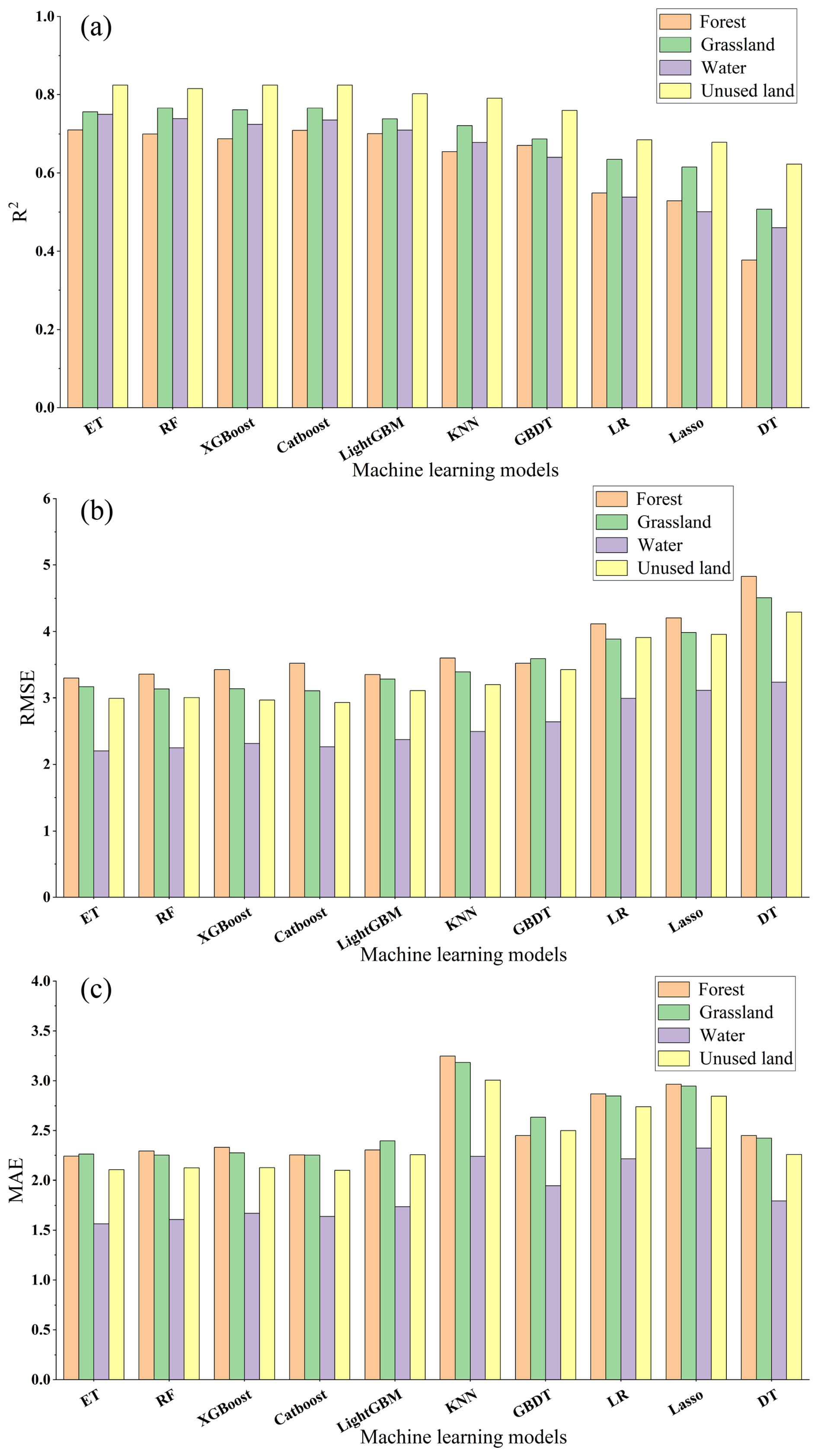
Figure 6 The results of the accuracy evaluation index of each model under four land cover types: (a) R², (b) RMSE; (c) MAE.

4.2 Evaluation of the accuracy of SD estimation

This study integrated AMSR-2 BT data with geographic variables (longitude and latitude), terrain factors (slope, aspect, elevation, and surface roughness), and other SD-related variables to construct AutoML-based SD estimation models for forest, grassland, water, and unused land regions. Using the Che_AMSR2_NSD dataset as the primary reference, the optimal model for each land cover type was applied to generate 500 m SD estimates (Auto_NSD) across the QTP for nine snow seasons from October 2012 to March 2021, covering a total of 1603 d. Ground-based SD observations were then employed to quantitatively evaluate the accuracy of the Auto_NSD results. In addition, the spatial distribution of snow cover was qualitatively assessed using cloud-free Landsat-8 optical imagery.

4.2.1 Evaluation of the overall accuracy of SD results

To evaluate the accuracy of the SD estimates derived from AutoML, 432 ground-based SD observations from odd dates in the QTP meteorological station dataset were used as validation data. Four quantitative metrics – R, RMSE, BIAS, and MAE – were employed to assess the accuracy of the SD estimates from 2012 to 2021. As shown in Fig. 7, the Auto_NSD results exhibit a strong agreement with meteorological station measurements, yielding an R² value of 0.71. The RMSE is 3.64 cm, indicating a slight overall underestimation ($\text{BIAS}=-\mathrm{1.72}$ cm). Meanwhile, the MAE remains relatively low at 2.93 cm, reflecting a high level of accuracy in the AutoML-based SD estimates.

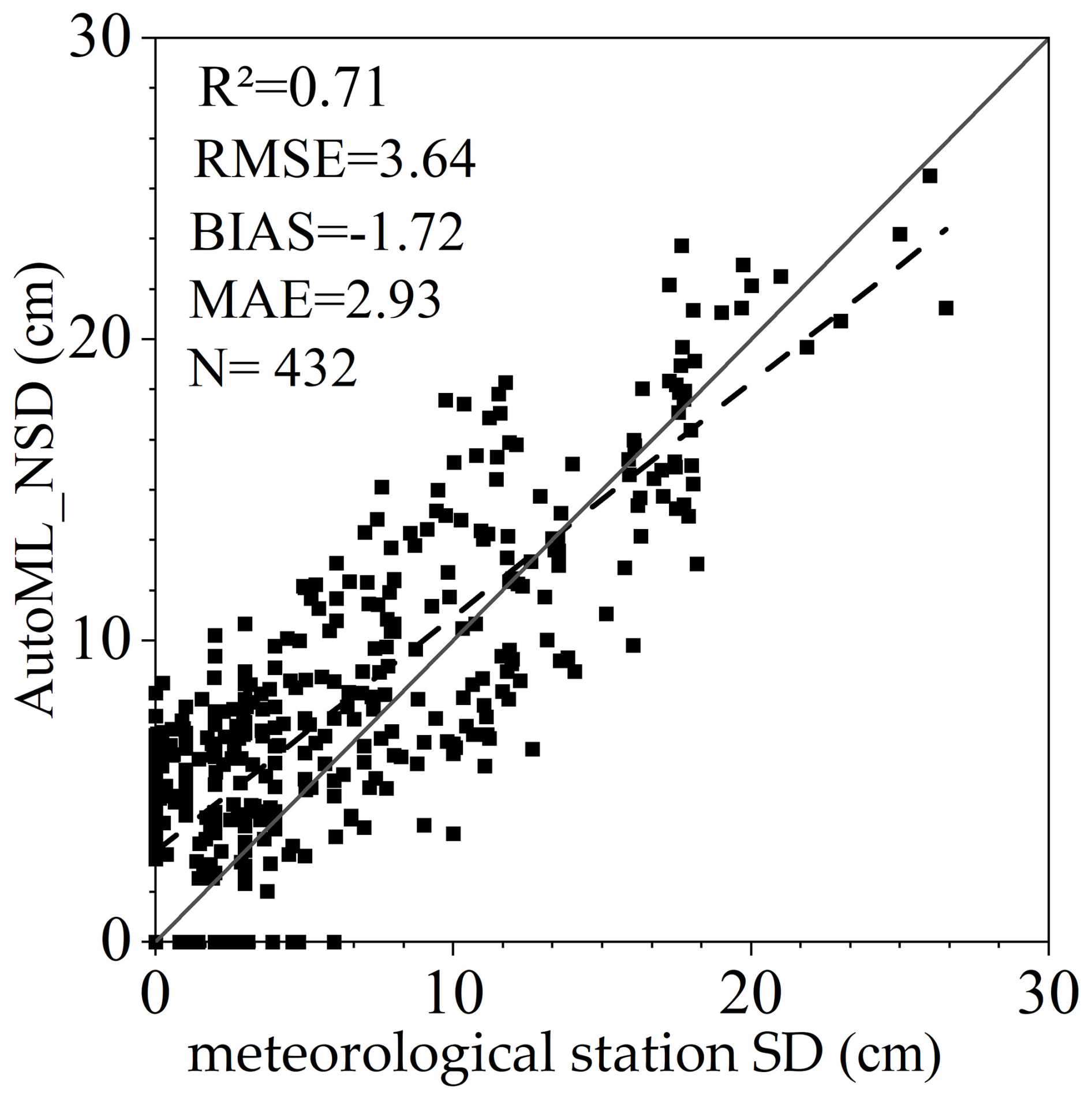
Figure 7 Scattered plot of SD observed by meteorological stations and SD estimation based on AutoML.

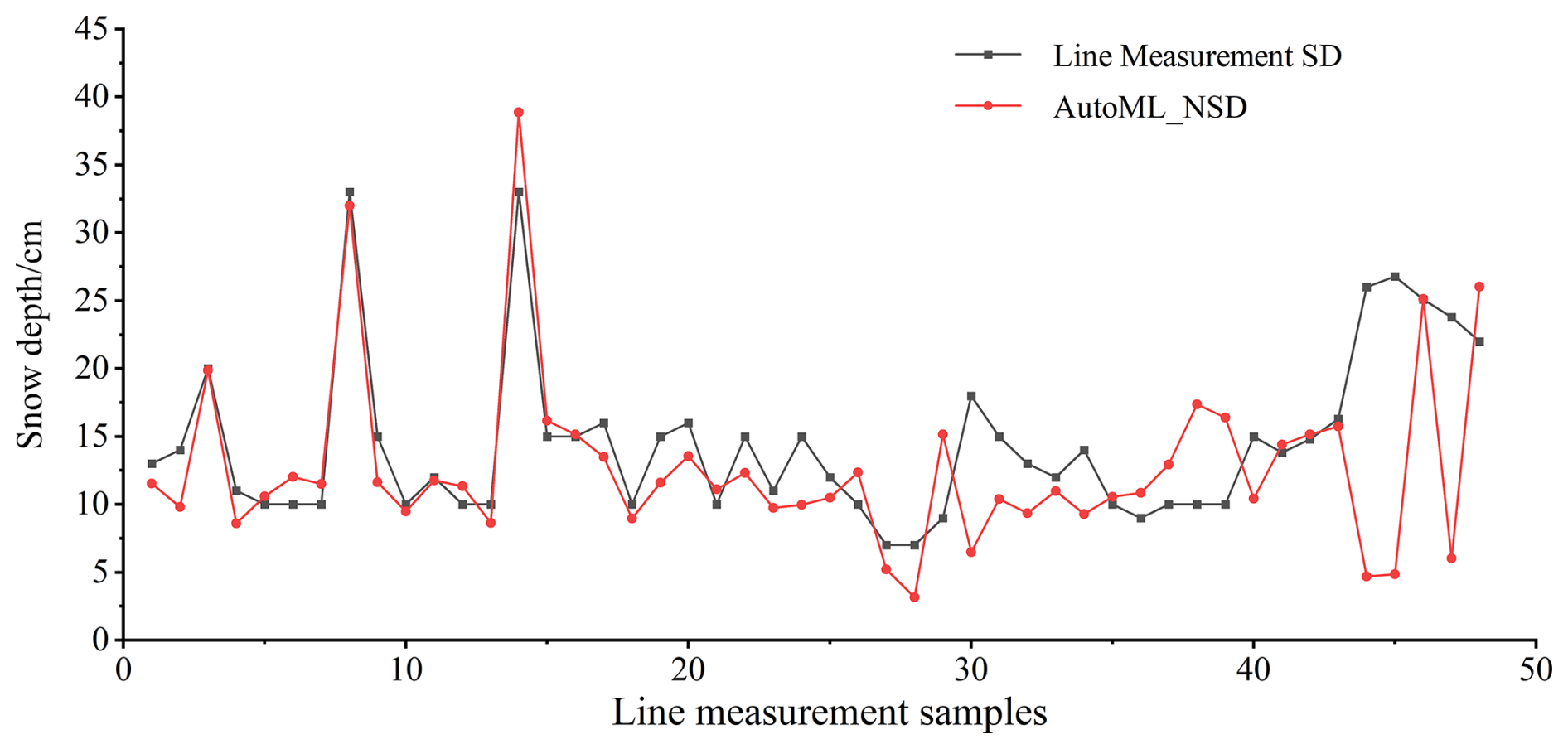
This study further employed snow survey data from the “Snow course dataset in typical snow area in China”, which provides SD observations from representative snow-covered regions across China. For the QTP, survey data collected along three routes during 2018–2019 were used, and SD measurements from 49 route points were compared with the corresponding Auto_NSD estimates. As illustrated in Fig. 8, the Auto_NSD results show relatively small discrepancies and consistent spatial patterns compared with the route-based measurements. The mean SD of the Auto_NSD dataset is 12.77 cm, with a maximum value of 38.88 cm, whereas the route observations yield a mean SD of 14.55 cm and a maximum value of 33 cm. Among the examined sample points, 30 cases (61 %) exhibit underestimation. The maximum underestimation error occurred on 20 January 2019 (21.93 cm), while the maximum overestimation error was 8.22 cm on 18 January 2019. The minimum absolute error was 0.15 cm, recorded on 7 December 2018.

Figure 8 Line chart of SD estimation and line measurement SD based on AutoML.

4.2.2 Evaluation of the spatial accuracy of SD results

Meteorological station SD observations were used as reference data to calculate the mean SD at each station and the corresponding mean SD derived from the Auto_NSD dataset. The spatial accuracy of Auto_NSD was then evaluated using RMSE and BIAS. As shown in Fig. 9a and b, the mean SD values from meteorological stations and Auto_NSD exhibit generally consistent spatial patterns. For 63 % of the stations, the difference in mean SD is within 5 cm. Stations such as Henan, Yege, and Zhenqin show small mean SD differences of −0.23, −0.34, and 0.43 cm, respectively. The largest mean SD discrepancy occurs at Niela station, reaching 23 cm. In March 2019, the observed SD at Niela station exceeded 120 cm, whereas the AutoML-based estimate was approximately 30 cm. This discrepancy may be related to limitations in the input data used for model training, as SD values at nearby sample points did not exceed 50 cm. With the exception of this particular station, the mean SD difference at other stations does not exceed 8 cm. Figure 9c and d present the spatial distribution of RMSE and BIAS between Auto_NSD estimates and meteorological station observations. Stations such as Henan, Yegor, Muli, Yanshiping, Haibei, Biru, and Dulan exhibit high accuracy, with RMSE values below 5 cm. Excluding Niela station, Jiali and Cuona show relatively lower accuracy, with RMSE values of 10.92 and 13.95 cm, respectively. A pronounced underestimation is evident at Niela station, while Cuona station shows a BIAS of −7.23 cm. In contrast, stations including Zhenqin, Wosai, Henan, and Yegor demonstrate close agreement with Auto_NSD, with BIAS values ranging between −0.5 and 0.5 cm. Overall, the spatial accuracy analysis indicates a clear relationship between SD magnitude and estimation uncertainty across the QTP.

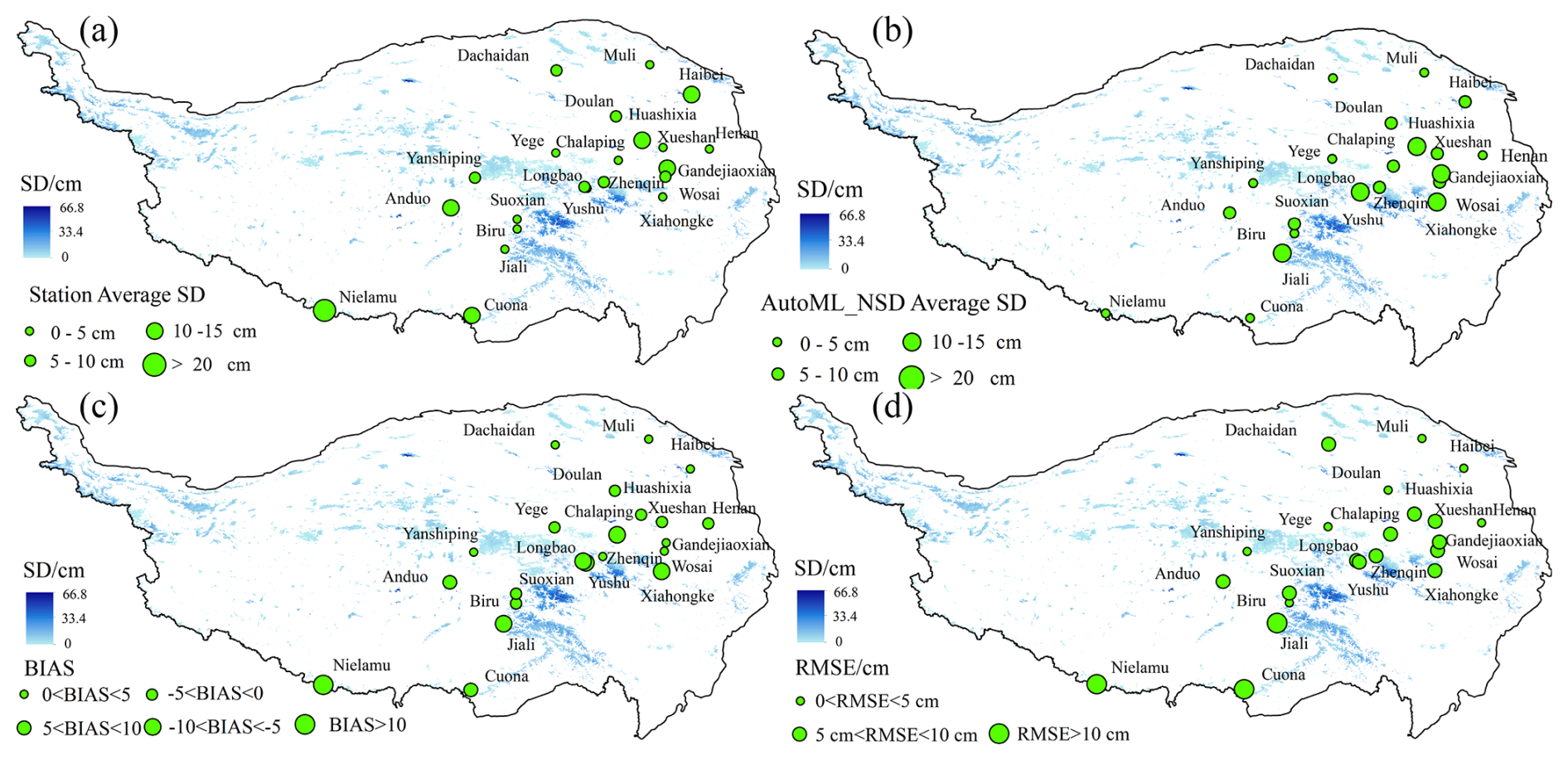
Figure 9 Spatial error distribution between Auto_NSD data and observed SD at meteorological stations: (a) average SD at meteorological stations; (b) the average SD of Auto_NSD data; (c) Auto_NSD data and the BIAS of SD at meteorological stations; (d) Auto_NSD data and RMSE of SD at meteorological stations.

To further examine the spatial distribution of snow cover across different periods and representative terrain conditions on the QTP, six cloud-free Landsat-8 images were selected according to satellite overpass times corresponding to the AutoML-estimated SD results. These images were compared with the corresponding Auto_NSD and downscaled SD datasets. As shown in Fig. 10, cyan indicates snow-covered areas and red denotes snow-free regions in the Landsat-8 imagery. Substantial temporal variability in snow distribution is evident. Landsat-8 images from 5 March 2013, 16 November 2015, and 9 November 2016 indicate relatively low snow coverage, mainly confined to lower-elevation areas, whereas images from 5 January 2014, 19 November 2017, and 25 February 2018 show more extensive snow cover, primarily in high-altitude mountainous regions. Overall, the spatial patterns of SD estimates are consistent with snow distributions observed in Landsat-8 imagery. However, regional differences are observed between Auto_NSD and downscaled SD data. For example, on 16 November 2015, Auto_NSD more accurately captures the observed snow distribution, while the downscaled SD exhibits noticeable rasterization effects. Similar rasterization artifacts are apparent in the downscaled SD data on 5 January 2014 and 19 November 2017. These differences likely result from the comprehensive integration of multiple SD-related factors in the AutoML framework, which allows for finer adjustment of pixel-level SD values. In summary, although both Auto_NSD and downscaled SD datasets effectively represent spatial SD patterns in mountainous regions, Auto_NSD provides a more spatially consistent depiction that aligns more closely with observed snow cover conditions.

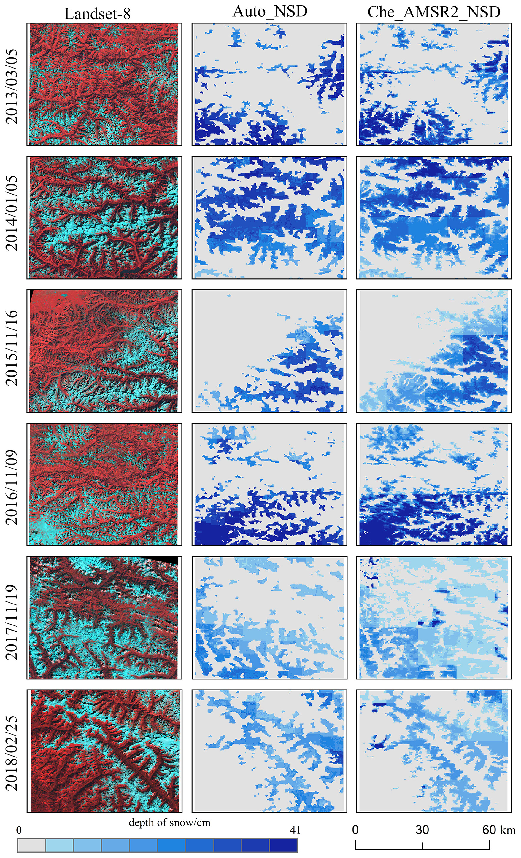
Figure 10 Comparison of the spatial distribution of Landsat-8 false-color composite images, SD estimation based on AutoML, and downscale SD estimation in 2012–2018.

4.3 Inverse correlation between temperature and SD

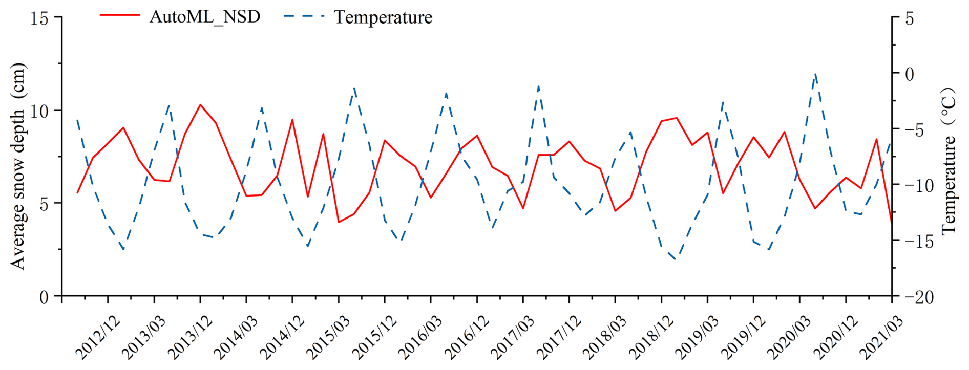
Statistical analysis of monthly mean SD time series was conducted using the Auto_NSD dataset for snow seasons on the QTP from 2012 to 2021. By integrating temperature observations, the temporal relationship between SD and temperature was further examined, as shown in Fig. 11. Overall, SD exhibits a consistent seasonal pattern during each snow season (October to March of the following year), characterised by an initial increase followed by a decrease. This pattern is inversely related to ERA5-Land temperature variations, which generally decrease during the early snow season and increase toward the end of the season. The snow season from October 2013 to March 2014 was selected as a representative period for detailed analysis. As temperatures increased, mean SD showed a gradual decline. In October 2013, the mean SD was 6.16 cm, corresponding to a mean monthly temperature of −2.82 °C. With the progressive decrease in temperature, the mean temperature in November dropped to −11.61 °C, while the mean SD increased to 8.71 cm. During December 2013 and January 2014, temperatures reached their lowest values of −14.49 and −14.81 °C, respectively, coinciding with maximum mean SD values exceeding 9 cm. From February to March, as temperatures gradually rose, SD decreased accordingly, reaching 5.37 cm in March. The highest mean SD occurred in December 2013 at an average temperature of −14.49 °C, whereas the lowest mean SD was recorded in October 2020, when the mean temperature exceeded 0 °C, reaching 0.046 °C.

Figure 11 Trends in Monthly Average SD during the Snow Seasons from 2012 to 2021 on the QTP.

5 Discussion

The QTP is characterised by its complex terrain, which includes a mosaic of mountains, plateaus, and basins. The distribution of meteorological stations across this region is sparse and uneven, adding to the challenge of obtaining accurate and comprehensive SD measurements. To address this issue, the study incorporated downscaled SD data (Che_AMSR2_NSD), which was used alongside ground-based SD observations as training data for the AutoML models. While this approach enhanced the precision of SD estimation in the QTP to some extent, the inherent uncertainty of the downscaled SD data has led to discrepancies between the downscaled and observed SD. In this study, meteorological station SD observation data were employed to assess the SD results obtained from AutoML estimations. The analysis considered different SD, snow periods, and land cover types. A comparative evaluation was conducted between the accuracy of the downscaled Che_AMSR2_NSD data and the Auto_NSD data, focusing on varying SD and snow accumulation periods. Additionally, the study explored the factors that influence the accuracy of SD inversion, providing insights into the limitations and potential improvements for SD estimation in this challenging region.

5.1 Impact of SD

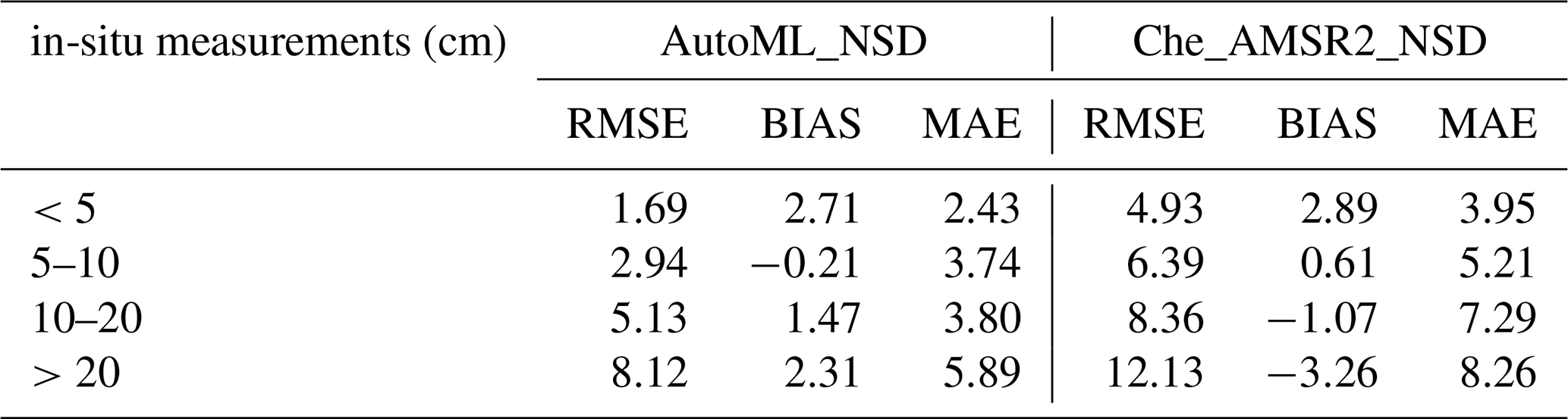
The accuracy of SD retrieval is closely related to the magnitude of SD. It is evident that measurements are more accurate in shallow snow conditions (less than 5 cm), with accuracy diminishing as SD increases. This trend aligns with similar findings from other studies in cold regions (Wang et al., 2022; Wei et al., 2022). A majority of observation stations in the QTP are located in regions with shallow SD (<10 cm). To facilitate analysis, this study categorises SD into four ranges: less than 5, 5–10, 10–20, and greater than 20 cm. The accuracy of SD estimation from both AutoML and downscaled SD methods was assessed using meteorological station SD measurements, as shown in Table 2. The results reveal that when SD is below 5 cm, Auto_NSD provides the most accurate estimations, with the lowest RMSE of 1.69 cm. The bias is 2.71 cm, and MAE is 2.43 cm, outperforming the Che_AMSR2_NSD data. For SD between 5 and 10 cm, RMSE for Auto_NSD is 2.94 cm, compared to 6.39 cm for Che_AMSR2_NSD. When the SD exceeds 20 cm, the estimation error increases. Specifically, RMSE for Auto_NSD is 6.43 cm higher compared to the less than 5 cm category. Nevertheless, AutoML-based SD estimations consistently show superior accuracy compared to Che_AMSR2_NSD data across all SD categories. Additionally, the AutoML model developed in this study outperforms existing ML-based methods for both shallow and deep snow conditions. For example, the RF model reported Yang et al. (2020) an RMSE of 4.2 cm for shallow snow (<5 cm) and 10.3 cm for deep snow (>20 cm) on the QTP. In comparison, the AutoML model reduces these values to 1.69 and 8.12 cm, respectively. This improvement stems from AutoML's strengths in model training and selection, which eliminate the need for extensive manual tuning and model screening.

Table 2 Accuracy indexes of SD estimation results at different measured SD.

It is clear that the accuracy of SD estimations declines as the standard deviation increases. This phenomenon can be attributed to the growing complexity of the snow layer. Snowmelt, which may occur both on the surface and within the snow layer, can alter temperature, humidity, and the dielectric constant beneath the snow (Han et al., 2024; Tanniru and Ramsankaran, 2023). This in turn leads to less reliable microwave radiation transmission, resulting in an increasing disparity between estimated SD and ground-based observations (Picard et al., 2022; Tanniru and Ramsankaran, 2023; Vuyovich et al., 2017). Additionally, microwave signals may undergo multiple reflections and scattering within the snow layer, which increases the complexity and instability of the received signals (de Gélis et al., 2025). Moreover, several studies suggest that when the SD exceeds a specific threshold, saturation issues can arise in the BT differences between 18 and 36 GHz (10 GHz) frequencies (de Gélis et al., 2025; Derksen et al., 2005; Huang et al., 2018).

5.2 Impact of Snow Accumulation Periods

As time progresses, the properties of snow undergo significant changes, primarily manifested in variations in snow density and particle size. Newly fallen snow is typically characterized by low density and small particle size. However, as snow accumulates and undergoes compaction and ice formation due to temperature fluctuations over time, the snow's density increases and particle size grows (Yang et al., 2020b). These variations in snow characteristics can significantly influence the performance of SD estimation models. In this study, the influence of different snow accumulation periods on SD estimation accuracy was investigated. Ground-based SD observation data were used as the “true values” for comparison. The RMSE, BIAS, and MAE between Auto_NSD and Che_AMSR2_NSD SD results were calculated for different snow accumulation periods, as illustrated in Fig. 12. A comparative analysis revealed that, during the accumulation period, the Auto_NSD data outperformed the downscaled SD data, with an RMSE that was 4.86 cm lower than that of Che_AMSR2_NSD. During the stable snow period, when snow properties are relatively stable and undergo minimal changes, the SD results demonstrated the highest accuracy, with RMSE values of 2.11 cm for Auto_NSD and 5.09 cm for Che_AMSR2_NSD. However, during the snowmelt period, SD estimation accuracy significantly declined. The RMSE for the most accurate Auto_NSD data was 5.21 cm, while the Che_AMSR2_NSD data exhibited an RMSE as high as 12.3 cm.

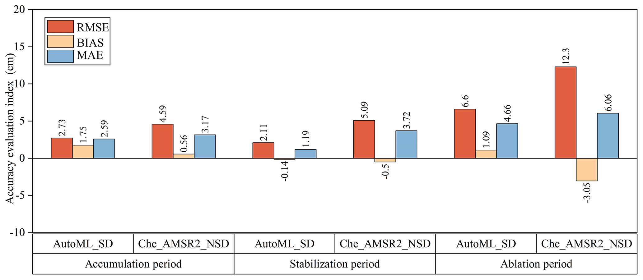
Figure 12 Comparison of the accuracy of SD data under different snow cover periods with the SD observation data of meteorological stations.

This decline in accuracy during the snowmelt period can be attributed to several factors. As temperatures rise during the snowmelt phase, snow transitions from dry snow to wet snow. Wet snow has a higher density and dielectric constant compared to dry snow, leading to attenuation of microwave radiation and weaker signal intensity (Picard et al., 2022; Vuyovich et al., 2017). The increased liquid water content in wet snow further contributes to enhanced reflection and scattering of microwave signals, which impedes the penetration of signals through the snow layer, thereby affecting SD estimation accuracy (de Gélis et al., 2025; Yang et al., 2020b).

5.3 Effect of land cover type on SD estimation

The influence of land cover type on the accuracy of SD estimation was found to vary across different environments. The model simulation results revealed that SD estimation accuracy was generally lower in forested regions. This can be attributed to the attenuation of microwave radiation as it passes through the vegetation canopy before reaching the snow-covered surface layer, which reduces the microwave signal strength detected by radiometers (Teubner et al., 2018; Foster et al., 1997). Additionally, the radiation emitted by the vegetation canopy and reflected by the snow layer further contributes to the attenuation of microwave signals, making snow characteristics more difficult to detect (Foster et al., 1997; Tanniru and Ramsankaran, 2023).

In contrast, most models performed satisfactorily in aquatic environments, although some uncertainty remained in SD estimation. The presence of ice layers in water bodies, particularly during the winter months when ice freezes, significantly impacts SD estimation accuracy. The physical properties of ice, including its high dielectric constant and low reflectivity, differ considerably from those of snow, altering the propagation and reflection of microwave radiation (Cheng et al., 2008). These differences in dielectric properties can disrupt the signal path and intensity, ultimately affecting the accuracy of SD estimation (Newman et al., 2014; Quéno et al., 2020). Furthermore, the lack of sufficient ground SD observation data near water bodies may have contributed to inaccurate SD predictions in these regions (Xu et al., 2023).

5.4 Uncertainty Analysis

This section evaluates the principal sources of uncertainty in SD estimation, including land cover representation, reference dataset selection, and snow cover identification, and examines their impacts on model stability and retrieval reliability.

The CNLUCC 2020 dataset is used to represent land cover conditions for 2012–2021. Land cover over the QTP changes slowly, particularly for dominant classes such as grassland, forest, and unused land, which occupy most of the region. Consequently, interannual variations during the study period are limited and are unlikely to substantially affect SD estimation at the spatial scale considered. Using a single and consistent land cover dataset also avoids uncertainties arising from inconsistencies among different products. Although local land use changes may introduce some uncertainty, their overall influence is limited because land cover is mainly used for categorical stratification rather than as a continuous predictor.

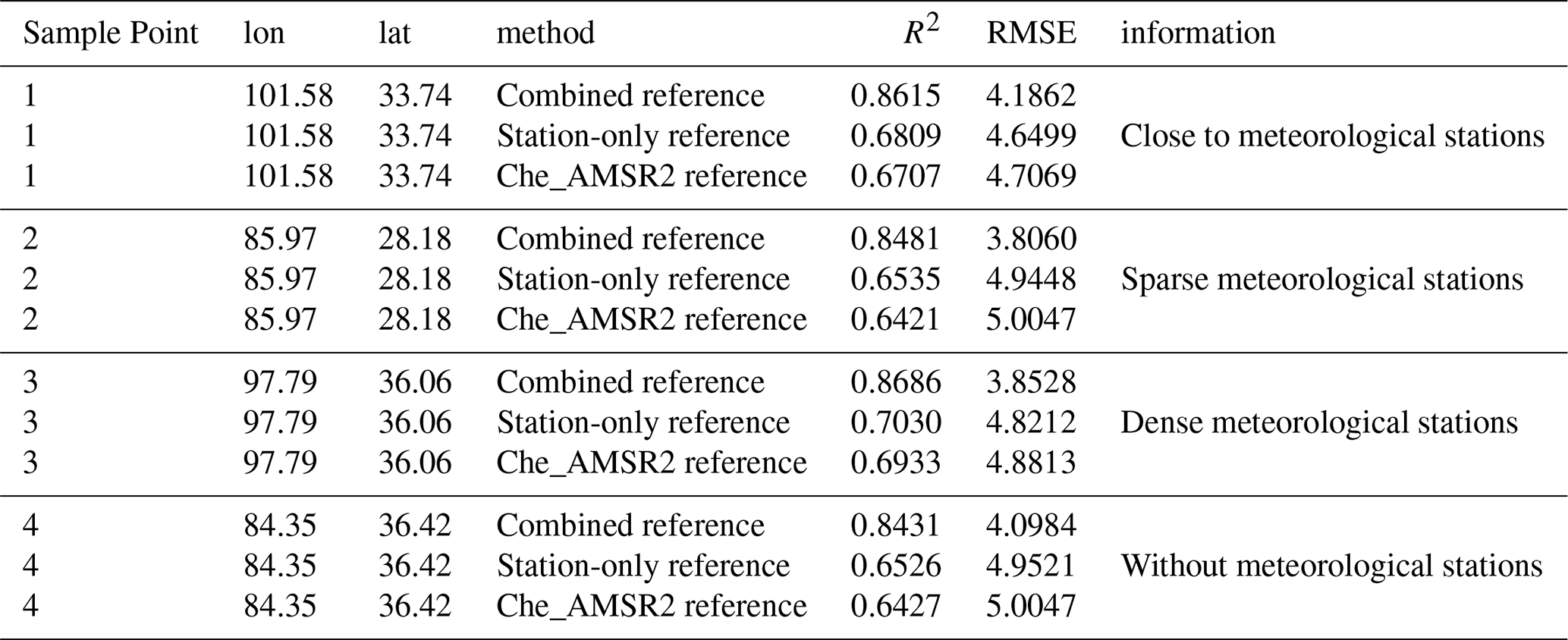
The Che_AMSR2_NSD SD product contains inherent uncertainties, including retrieval errors over complex terrain and potential temporal mismatches with in situ observations. Therefore, it serves as a supplementary reference rather than strict ground truth, particularly in regions with sparse meteorological stations. To evaluate the impact of reference data uncertainty, four representative sites across the QTP with contrasting station densities were selected, and model performance was assessed under three reference strategies: station-only observations, coarse-resolution Che_AMSR2 SD data, and a combined reference integrating station observations with Che_AMSR2_NSD (Table 3). The combined strategy consistently performs best, with R² values of 0.84–0.87 and RMSE of 3.8–4.2 cm, compared to lower R² (0.64–0.70) and higher RMSE (4.6–5.0 cm) for the other two strategies. These results indicate that incorporating Che_AMSR2_NSD mitigates the limitations of sparse stations and coarse-resolution satellite data. Direct comparisons between Che_AMSR2_NSD and ground-based observations show a moderate correlation with systematic biases (R=0.72, Fig. 13), suggesting potential uncertainty propagation into SD estimation. Nevertheless, the AutoML-based framework maintains stable performance across reference scenarios, demonstrating robustness to reference data uncertainty.

Table 3 Sensitivity of SD estimation performance to different reference data sources at representative sites across the QTP.

Figure 13 Scattered plot of SD observed by meteorological stations and SD by Che_AMSR2_NSD.

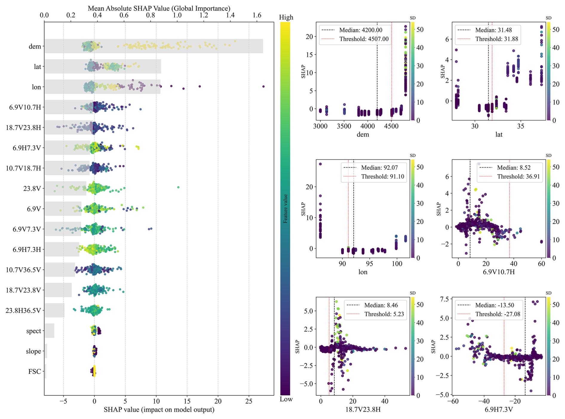
Uncertainty associated with snow cover identification is comparatively minor. The daily cloud-free snow cover product is used solely as a binary mask, with SD set to zero for snow-free pixels and snow-covered pixels processed through the proposed framework. It is not included in model training or validation; thus, its uncertainties do not directly propagate through the regression process, affecting results only through potential snow/no-snow misclassification. SHAP-based feature importance and sensitivity analyses (Fig. 14) show that elevation and latitude dominate model predictions, while snow cover–related variables have near-zero mean Shapley values. SHAP dependence plots further confirm that FSC variations do not induce systematic changes in SD estimates relative to terrain and geographic predictors. Overall, snow cover–related uncertainties play a secondary role in the uncertainty budget, and the robustness of the proposed framework is primarily determined by dominant predictors rather than snow cover identification errors.

Figure 14 SHAP dependence plots.

5.5 Shortcomings and prospects

This study introduces a novel methodology for estimating SD in the QTP, utilizing AutoML techniques to refine the process. By enhancing the spatial resolution of SD data and incorporating various factors that influence SD inversion, the study has developed optimized models for four key land cover types, effectively capturing the heterogeneity of SD distributions across different terrains. This approach has proven especially valuable for rapid SD monitoring in mountainous regions, where terrain complexity often presents significant challenges.

However, several limitations of this study should be acknowledged. (1) First, while topographical factors were thoroughly considered, other variables affecting SD retrieval, such as snow density, grain size, liquid water content, and vegetation canopy, were not incorporated. These factors can significantly impact SD retrieval accuracy (Ni et al., 2024; Zhang et al., 2021). The study's reliance on station observation data, which are sparsely distributed across the QTP from 2012 to 2021, limited the incorporation of these additional factors into the AutoML inversion process. As a result, these factors were excluded from the analysis. (2) Second, the QTP is characterized by substantial spatiotemporal heterogeneity in SD, with variations in SD distribution observed across different terrains, altitudes, and stages of the snow season. Although ground-based SD observations from multiple locations were used to verify the accuracy of the ML model estimates, the limited coverage of observational data prevented the inclusion of SD observations from a broader range of terrain types. (3) Third, the feature selection process employed a traditional approach based on correlation coefficients to identify influential factors. Future research will explore more advanced feature selection techniques, such as feature importance and variance inflation factor, to improve model accuracy. (4) Finally, while this study briefly explored the relationship between SD and temperature, it did not delve into deeper aspects of this relationship. Future studies will aim to examine the seasonal patterns, spatial heterogeneity, and sensitivity of SD to temperature variations in the QTP.

6 Conclusion

The present study focused on the QTP, employing an ML model with downscaled SD data, ground SD observations, and 19 SD-influencing factors as input data. The input data samples were trained under four distinct types of snow cover (forest, grassland, water, and unused land), and the optimal ML model was selected for each type of snow cover using ten-fold cross-validation. Consequently, SD datasets for the QTP from 2012 to 2021 were obtained. A comprehensive evaluation was conducted to assess the precision of Auto_NSD and Che_AMSR2_NSD SD data, including both quantitative and qualitative analyses. The findings suggested that (1) the SD estimates derived from ML techniques exhibited superior accuracy in characterizing the snow distribution in the QTP region, closely matching ground observations, with R²=0.71, RMSE=3.64 cm, $\text{BIAS}=-\mathrm{1.72}$ cm, and MAE=2.93 cm; (2) The SD estimation accuracy of ML models varies across different underlying surfaces. Unused land (CatBoost, R²=0.82) exhibited the highest accuracy, followed by grassland (CatBoost, R²=0.77, RMSE=3.11 cm), water (ET, R²=0.75, RMSE=2.20 cm), and forest (XGBoost, R²=0.71, RMSE=3.30 cm); (3) A comparison with snow cover ranges identified through Landsat-8 imagery demonstrated that both SD datasets were able to reflect the detailed spatial features of snow distribution in mountainous regions. However, the Auto_NSD data provided a more consistent description of SD distribution compared to the real SD distribution, meeting the monitoring requirements for SD in mountainous regions.