Ice motion across incised fjord landscapes

The dynamic behaviour of ice-sheet motion over rough landscapes is poorly understood, with most ice-sheet models prescribing a bed smoother than reality, which does not fully capture topographic features. Subglacial fjords striking obliquely to the palaeo flow direction are an end member of this misrepresentation, but are ubiquitous beneath the western margin of the palaeo Scandinavian Ice Sheet, and provide a useful proxy for areas of the present-day Greenland Ice Sheet. Here, we consider Veafjorden as a characteristic western Norwegian fjord where striations clearly evidence palaeo perpendicular ice flow, and perform 3D thermodynamically-coupled ice-motion simulations across a range of orientations. For perpendicular flow, Moffatt eddies, or spiralling flows, occur within a thick layer of temperate ice in the fjord hollow with reverse-direction slip at the fjord base. Area-averaged driving stress in simulations with high-resolution topography and fjord-perpendicular flow is ∼41 %–89 % greater than in simulations with smoothed control topography for an equivalent surface velocity. In comparison, simulations with fjord-perpendicular flow show ∼28 %–45 % greater area-averaged driving stress than simulations with fjord-parallel flow. The steep slopes of fjords and other similar features also provide a clear physically-based example for why bounded basal traction relationships may not hold at the macro scale in rough settings. Similar topographic features may explain surface velocity variations at many locations towards the margins of the Greenland Ice Sheet, and imply that the role of anisotropic roughness in resisting ice-sheet motion may be under-represented in models.

1 Introduction

Basal topography exerts a critical control on ice-sheet motion at all scales considered (Kyrke-Smith et al., 2018; Helanow et al., 2021; Castleman et al., 2022; Frank et al., 2022; Wernecke et al., 2022; Law et al., 2023), but its influence at the intermediate scale – between the 0.5–25 m scale typically used to determine sliding parametrisations and the 400–4000 m scale typical of ice-sheet model fidelity – is particularly poorly understood. Notably, the ice-motion influence of incised fjord landscapes remains almost entirely unexplored. This landscape characterises the terrestrial western margin of the palaeo Scandinavian Ice Sheet and provides a reasonable proxy for marginal areas of the Greenland Ice Sheet (GrIS) which share geological and topographic similarities (e.g. Gee et al., 2008; Christ et al., 2023; Paxman et al., 2024), as well as regions of the Antarctic Ice Sheet (AIS) such as the Aurora Subglacial Basin (Young et al., 2011). In western Norway, glacial striations (Kleman et al., 1997; Mangerud et al., 2019) and paleoglacial flow directions (Jungdal-Olesen et al., 2024) show perpendicular ice flow over deep subglacial fjords, as well as in oblique and parallel orientations (Fig. 1). The implications for ice motion in these flow scenarios remain unclear.

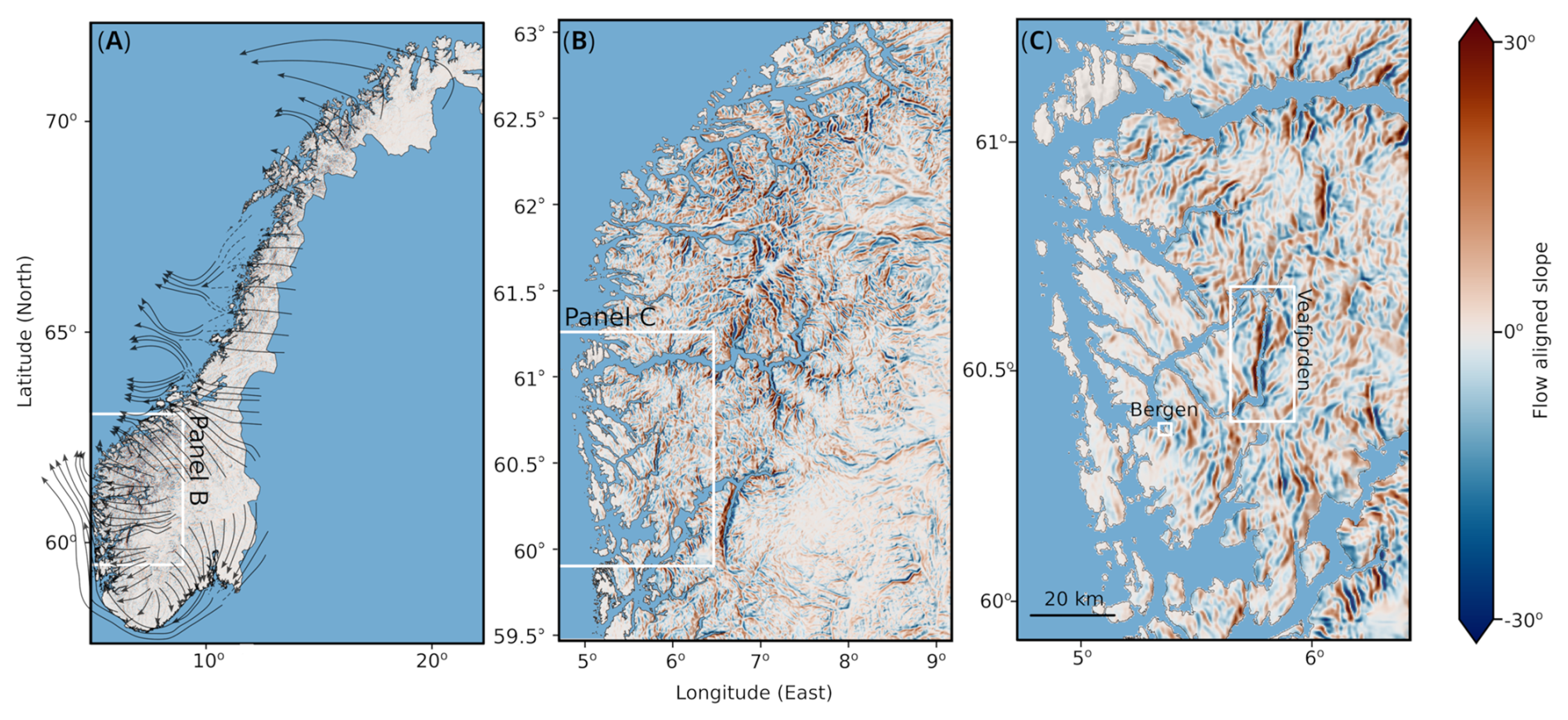
Figure 1 Slope calculated using the flow direction output of Jungdal-Olesen et al. (2024) for 32 kyr ago with Copernicus GLO-30 DEM data (Copernicus DEM, 2024). Positive values indicate an increase in elevation along the flow direction. Note that the maximum resolution of 60 m in panel (C) means that some small features (i.e. cliffs) may not be accurately resolved. Flow arrows in panel (A) adapted from Ottesen et al. (2005).

Here, we focus on Veafjorden close to the city of Bergen, Norway (Fig. 2) as a characteristic example with a relief of ∼1300 m, and a narrow ∼2 km width. Striation markings on both sides of Veafjorden confirm near-perpendicular flow across the fjord around 15 kyr ago (Mangerud et al., 2019). The Norwegian fjords were likely incised into pre-existing river valleys and geological weaknesses through erosion as the Scandinavian Ice Sheet grew and shrank, but not while the ice sheet was at its fullest extent (Harbor et al., 1988; Harbor, 1992; Briner et al., 2008; Bernard et al., 2021; Paxman, 2023; Reilly, 2023; Jungdal-Olesen et al., 2024; Egholm et al., 2017). In common with a comparable study from south-west South America (Glasser and Ghiglione, 2009), it may be that geological factors, rather than dynamic self-organisation of ice streams (Kessler et al., 2008), exert a first-order control on fjord orientation.

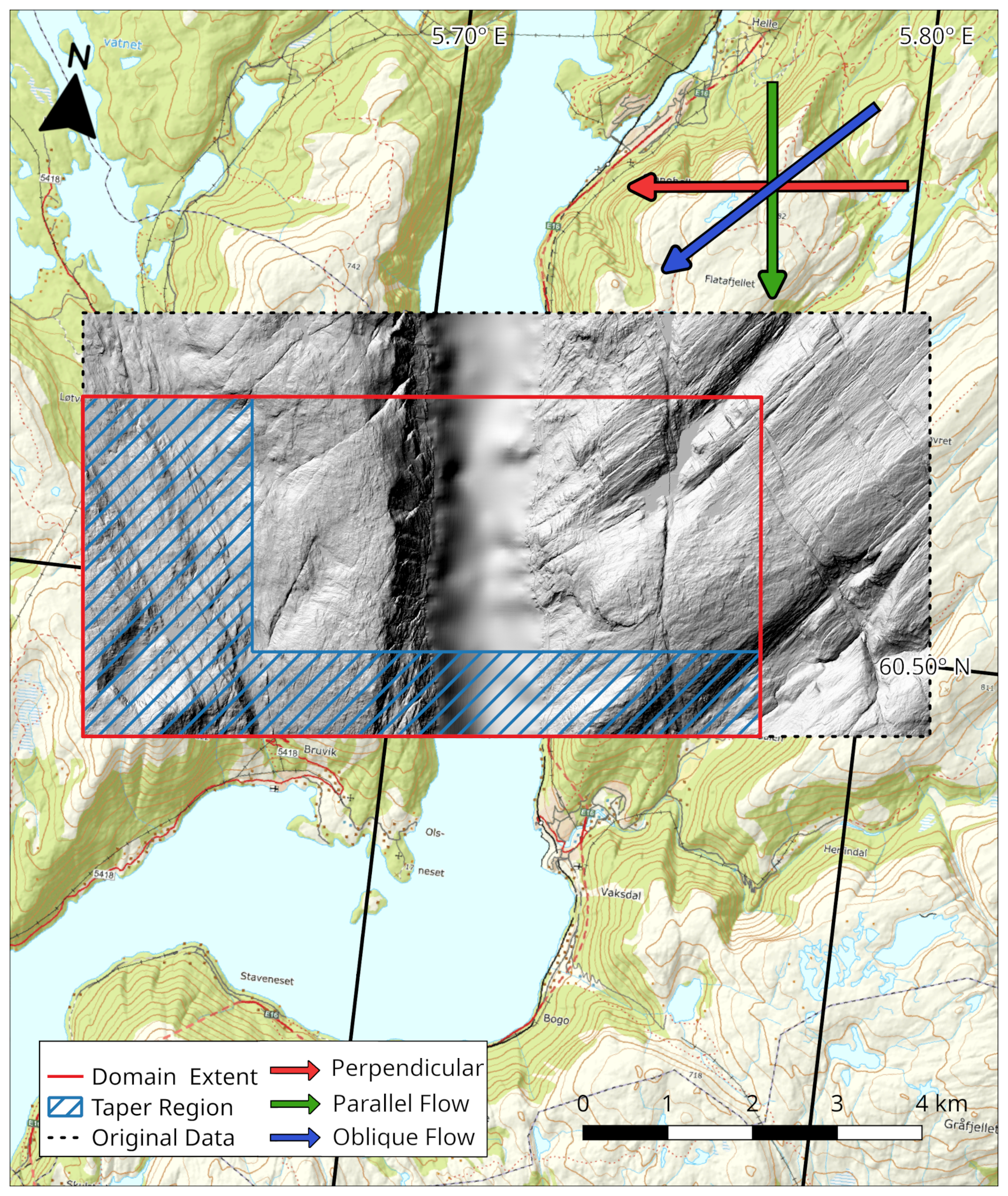
Figure 2 DEM of Veafjorden. The blue hatched area show the tapering region used in all simulations. The red, blue and green arrows displays the simulated flow directions. Perpendicular flow (red arrow) have been dated to 15 kyr BP and parallel flow (green arrow) at 11.5 kyr BP (Mangerud et al., 2019). Elevation data from the Norwegian Mapping Authority (Kartverket, 2024a, b).

Ice motion perpendicular to idealised subglacial valleys has previously been modelled in 2D and 3D (Gudmundsson, 1997; Meyer and Creyts, 2017), with Meyer and Creyts (2017) investigating the role of a critical angle in V-shaped valleys to predict the onset of Moffatt eddies (spiralling ice flow that form in topographic hollows). However, these studies did not include temperate ice rheology or rate-dependent resistance for slip at the ice-bed boundary, with simplified 2D topography in the case of Gudmundsson (1997) and simplified 3D topography and a 2D radar transect profile in the case of Meyer and Creyts (2017). Here, we incorporate these additional processes and consider fast ice motion for a section of the palaeo Scandinavian Ice Sheet over 3D high-resolution digital elevation data. In order to assess the difference in controls on ice motion between this high-resolution topography, and the smoother bed products used to model the GrIS and AIS (BedMachine and BedMap), we create a smoothed representation of Veafjorden (henceforth referred to as the smoothed control topography). This substitute provides the basis to examine the impact of the generally low fidelity elevation models presently in use.

Our ensemble consists of 16 simulations, each with a unique ice flow scenario. The varying parameters are (1) target surface velocity, (2) flow direction – parallel, oblique and perpendicular to the fjord incision (See Fig. 2) – and (3) plateau ice thickness, ice thickness measured from the highest point in our domain. The flow direction is varied both to simulate the historical shift in flow angle during deglaciation, and to assess how anisotropic bedrock influence ice dynamics. We also perform 4 comparison simulations with the smoothed topography. The smoothed control topography simulations have perpendicular flow direction while target surface velocity and plateau ice thickness are still varied. By simulating Veafjorden with both the smoothed control topography and the high-resolution topography, we reveal the influence of realistic anisotropic basal conditions and limited bed topography fidelity in ice-sheet models.

Over a single glacial cycle, the orientation of ice motion varies (Jungdal-Olesen et al., 2024), while the landscape remains effectively immutable. The simulations presented here, and consideration of how these extend to the broader palaeo Scandinavian Ice Sheet, indicate that over anisotropic topography complex basal motion patterns should be expected as the norm rather than the exception. Finally, while our simulations reveal ice dynamics over fjords in great detail, considerations of simple aspects of fjord geometry point towards the influence such landscapes should exert on intermediate, or macro, scale sliding relationships.

2 Methods

We model 3D ice motion over an 8 km by 4 km rectangular domain covering Veafjorden (Fig. 2). The Digital Elevation Model (DEM) was constructed at a resolution of 20 m with data from Kartverket (The Norwegian Mapping Authority), combining terrestrial data at 1 m (Kartverket, 2024b), with the fjord bathymetry interpolated from a 50 m resolution data set (Kartverket, 2024a). To conform to the model's periodic boundary conditions the inflow and outflow boundaries must match. We achieved this using a tapering algorithm following Helanow et al. (2021), with one third of the down-flow length and width of the domain added as a tapering region that then matches the topography at the inflow boundary (Fig. 2). We applied a Gaussian filter with a standard deviation of 1.5 to the DEM to remove artifacts and sharp edges which can present model stability issues (Law et al., 2023). Additionally, a smoothed control topography was created for comparison runs by applying a Gaussian filter with a standard deviation of 50 grid cells to the original DEM.

The domain was discretised with gmsh for Elmer/Ice Version 9.0 (Gagliardini et al., 2013) using a triangular mesh with a representative element side length of 25 m and 20–30 vertical layers with resolution increasing towards the base. The smoothed control topography mesh has a representative side length of 100 m and 15 vertical layers with 500 m plateau ice thickness. In a first stage, the free surface is allowed to vary and the inflow and outflow and two lateral boundaries are matched periodically for velocity, stress, and free-surface position. This simulation stage runs until a steady state is reached and surface elevation no longer varies. In the second stage, the free surface and the inflow velocity fields are fixed and the enthalpy field is allowed to evolve without a periodic boundary condition requirement. Outflow/side boundaries are set at lithostatic pressure/zero flux depending on simulation orientation (Fig. A1).

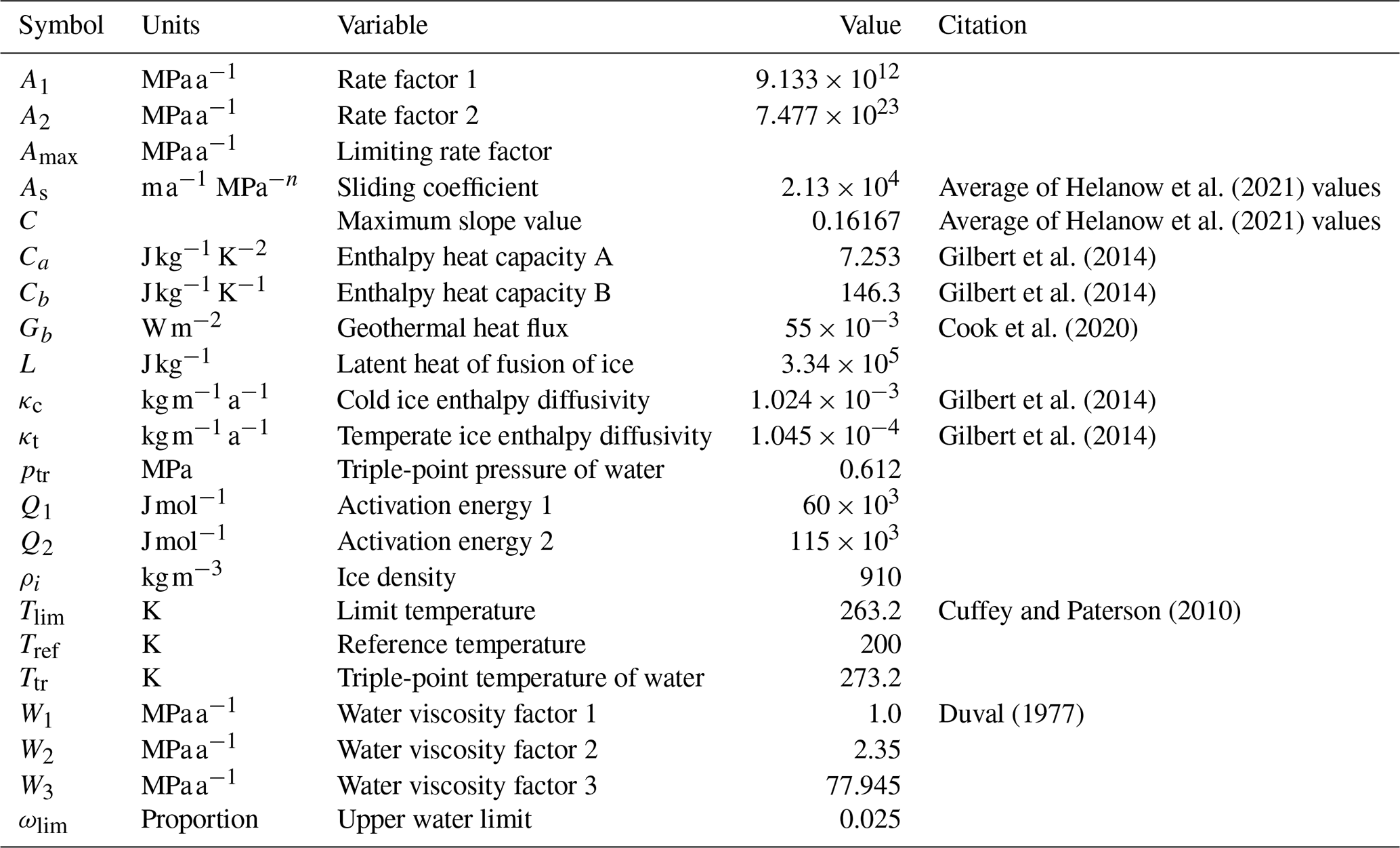
The central equations and boundary conditions follow Law et al. (2023) with minor adjustments to geometric set up. Table A1 lists all parameter values. We solve the standard Stokes equations for ice flow

$$\begin{array}{}\text{(1)}& {\displaystyle }& {\displaystyle }\mathrm{\nabla }\cdot \mathit{u}=\mathrm{0}\text{ (conservation of mass)}\text{(2)}& {\displaystyle }& {\displaystyle }\mathrm{\nabla }\cdot \mathit{\tau }-\mathrm{\nabla }p=-\mathit{\rho }\mathit{g}\text{ (conservation of momentum)}\end{array}$$

where u (m a⁻¹) is the velocity vector, τ (MPa) is the deviatoric stress tensor, p (MPa) is ice pressure, ρ (kg m⁻³) is the ice density and g is the gravity vector described as

$$\begin{array}{}\text{(3)}& {\displaystyle }{\displaystyle }\mathit{g}=\left[g\text{ sin}\right(\mathit{\theta }),\mathrm{0},-g\text{ cos}(\mathit{\theta }\left)\right]\end{array}$$

where g=9.81 m s⁻² and θ is the domain slope. In simulations, the x axis is oriented perpendicular to the fjord incision, and the y axis along the fjord. The z axis is normal to the horizontal plane, and does not match the g vector. Adjusting the orientation of g removes the requirement for vertical displacement of periodic inflow-outflow boundaries.

Stress is related to strain using the Nye–Glen isotropic flow law (Nye, 1953; Glen, 1955; Cuffey and Paterson, 2010):

$$\begin{array}{}\text{(4)}& {\displaystyle }{\displaystyle }\dot{\mathit{ϵ}}=A{\mathit{\tau }}_{\mathrm{e}}^{n-\mathrm{1}}\mathit{\tau }\end{array}$$

where $\dot{\mathit{ϵ}}$ (s⁻¹) is the strain rate tensor, ${\mathit{\tau }}_{\mathrm{e}}^{\mathrm{2}}=\frac{\mathrm{1}}{\mathrm{2}}\text{tr}\left({\mathit{\tau }}^{\mathrm{2}}\right)$ (MPa) is the effective stress in the ice, n is the flow exponent set to 3. The creep parameter, A (${\mathrm{MPa}}^{-\mathrm{3}}{\mathrm{a}}^{-\mathrm{1}}$), varies depending on whether ice is above or below the pressure melting point T_m. For ice below T_m, A is set using the homologous temperature, T_h (K), while ice above T_m, is determined by the water fraction ω:

$$\begin{array}{}\text{(5)}& {\displaystyle }{\displaystyle }A=\left\{\begin{array}{ll}{A}_{\mathrm{1}}\exp \left(\frac{Q_{\mathrm{1}}}{R{T}_{\mathrm{h}}}\right),& T_{\mathrm{h}}\le T_{\text{lim}}\\ A_{\mathrm{2}}\exp \left(\frac{Q_{\mathrm{2}}}{R{T}_{\mathrm{h}}}\right),& T_{\text{lim}}<T_{\mathrm{h}}<T_{\mathrm{m}}\\ (W_{\mathrm{1}}+W_{\mathrm{2}}\mathit{\omega }\times \mathrm{100})W_{\mathrm{3}},& T_{\mathrm{h}}\ge T_{\mathrm{m}}\text{ and }\mathit{\omega }<{\mathit{\omega }}_{\text{lim}}\\ A_{\text{max}},& \mathit{\omega }\ge {\mathit{\omega }}_{\text{lim}}\end{array}\right.\end{array}$$

where $T_{\mathrm{m}}\left(p\right)=T_{\text{tr}}-\mathit{\gamma }(p-p_{\text{tr}})$ and γ (K MPa⁻¹) is the Clausius–Clapeyron constant, and T_tr and p_tr are the temperature and pressure triple points for water, respectively. A₁ and A₂ (MPa a⁻¹) are rate factors, Q₁ and Q₂ (J mol⁻¹) are activation energies for T≤T_lim and $T_{\text{lim}}<T<T_{\mathrm{m}}$, respectively, where T_lim is the limit temperature. R (J mol⁻¹) is the gas constant, W₁, W₂, and W₃ (MPa a⁻¹) are water viscosity factors (constant for all simulations) with default values from Haseloff et al. (2019) adapted from Duval (1977). The liquid water fraction limit, ω_lim is set to 2.5 % following experiments of Adams et al. (2021). If ω_lim is exceeded then A is limited to a maximum value A_max. Very recent studies propose n=1, or different relationships for A for temperate ice (Schohn et al., 2025; Roldán-Blasco et al., 2025), but we leave exploration of these parameters for a future study. Values for these and subsequent parameters are provided in Table A1.

Within the Elmer/Ice EnthalpySolver (Gilbert et al., 2014), specific enthalpy, H (J kg⁻¹), is used as the state variable and is related to T and ω as

$$\begin{array}{}\text{(6)}& {\displaystyle }{\displaystyle }H(T,\mathit{\omega })=\left\{\begin{array}{ll}\begin{array}{rl}{\displaystyle }& {\displaystyle \frac{\mathrm{1}}{\mathrm{2}}}{C}_a\left(T^{\mathrm{2}}-{T_{\text{ref}}}^{\mathrm{2}}\right)\\ {\displaystyle }& {\displaystyle }+C_b\left(T-T_{\text{ref}}\right),\end{array}& H<H_{\mathrm{m}}\left(p\right)\\ \mathit{\omega }L+H_{\mathrm{m}},& H\ge H_{\mathrm{m}}\left(p\right)\end{array}\right.\end{array}$$

where C_a (J ${\mathrm{kg}}^{-\mathrm{1}}{\mathrm{K}}^{-\mathrm{2}}$) and C_b (J ${\mathrm{kg}}^{-\mathrm{1}}{\mathrm{K}}^{-\mathrm{1}}$) are enthalpy heat capacity constants, L (J kg⁻¹), is the latent heat capacity of ice, $H_{\mathrm{m}}\left(p\right)=\frac{\mathrm{1}}{\mathrm{2}}{C}_a\left(T_{\mathrm{m}}(p{)}^{\mathrm{2}}-{T_{\text{ref}}}^{\mathrm{2}}\right)+C_b\left(T_{\mathrm{m}}\left(p\right)-T_{\text{ref}}\right)$ is the specific enthalpy at the pressure melting point, and T_ref is the reference temperature.

At each time step, the enthalpy field is evolved until a steady-state is reached and is calculated as

$$\begin{array}{ll}{\displaystyle }\mathit{\rho }\left({\displaystyle \frac{\partial H}{\partial t}}+\mathit{u}\cdot \mathrm{\nabla }H\right)=& {\displaystyle }\mathrm{\nabla }\left(\mathit{\kappa }\mathrm{\nabla }H\right)+\text{tr}\left(\mathit{\tau }\dot{\mathit{ϵ}}\right)\\ \text{(7)}& {\displaystyle }& {\displaystyle }\text{(conservation of energy)}\end{array}$$

where $\text{tr}\left(\mathit{\tau }\dot{\mathit{ϵ}}\right)$ is the strain heating term and κ (kg ${\mathrm{m}}^{-\mathrm{1}}{\mathrm{s}}^{-\mathrm{1}}$) is the enthalpy diffusivity defined as

$$\begin{array}{}\text{(8)}& {\displaystyle }{\displaystyle }\mathit{\kappa }=\left\{\begin{array}{ll}{\mathit{\kappa }}_{\mathrm{c}},& H<H_{\mathrm{m}}\left(p\right)\\ {\mathit{\kappa }}_{\mathrm{t}},& H\ge H_{\mathrm{m}}\left(p\right)\end{array}\right.\end{array}$$

where κ_c and κ_t are enthalpy diffusivities for cold and temperate ice respectively (Schoof and Hewitt, 2016), meaning that water movement within the temperate ice is assumed to be a diffusive process.

The change in the position of the free surface, s, is calculated as

$$\begin{array}{}\text{(9)}& {\displaystyle }{\displaystyle \frac{\mathit{\delta }s}{\mathit{\delta }t}}+u_x{\displaystyle \frac{\mathit{\delta }s}{\mathit{\delta }x}}+u_y{\displaystyle \frac{\mathit{\delta }s}{\mathit{\delta }y}}=u_z\end{array}$$

in the Elmer/Ice FreeSurfaceSolver where u_x, u_y, and u_z are components of u.

The lower boundary velocity is set to zero normal to the surface (impenetrability condition at base):

$$\begin{array}{}\text{(10)}& {\displaystyle }{\displaystyle }\mathit{u}\cdot \mathit{n}=\mathrm{0}\end{array}$$

where n is the normal vector to the bedrock. Basal traction τ_b is calculated following Helanow et al. (2021) as:

$$\begin{array}{}\text{(11)}& {\displaystyle }{\displaystyle }{\mathit{\tau }}_{\mathrm{b}}=C{N}_{\mathrm{e}}{\left({\displaystyle \frac{u_{\mathrm{b}}^{-n+\mathrm{1}}}{u_{\mathrm{b}}+A_{\mathrm{s}}{C}^n{N}_{\mathrm{e}}^n}}\right)}^{\frac{\mathrm{1}}{n}}{u}_{\mathrm{b}}\end{array}$$

where C (dimensionless) is a parameter dependant on basal morphology (Helanow et al., 2021). $N_{\mathrm{e}}=p_{\mathrm{i}}-p_{\mathrm{w}}$ (MPa) is the effective pressure where p_i (MPa) is the ice overburden pressure and p_w (MPa) is the subglacial water pressure, with N set at 24 % of p_i following Law et al. (2023). u_b (m a⁻¹) is the basal velocity tangential to the ice-bed interface. The flow exponent n is the same as for the strain rate and set as 3. A_s (m ${\mathrm{a}}^{-\mathrm{1}}{\mathrm{MPa}}^{-\mathrm{3}}$) is the average sliding coefficient based on six values from Helanow et al. (2021).

2.1 Simulation ensemble

We simulate variations in flow direction, target surface velocity, and the thickness of ice over the plateau (measured from the highest point within the domain), as well as a smoothed control run with ice motion perpendicular to the fjord. We selected two plateau ice thicknesses, 500 and 1000 m, both within the modelled plateau ice thickness of previous studies (Svendsen and Mangerud, 1987; Mangerud et al., 2019) and which provide a reasonable range for exploring the role of plateau ice thickness on flow patterns before fjord geometry begins to influence flow direction (Reilly, 2023). Two target surface velocities were selected, 450 and 850 m a⁻¹, based on the surface velocity at bore-hole locations with matching ice thickness in Greenland (Løkkegaard et al., 2023). Three flow directions are simulated, perpendicular (90°), oblique (45°) and parallel (0°). An overview of all simulations can be found in Table 1 and Fig. 3.

Table 1 An overview of simulated scenarios and results. Flow direction is relative to the orientation of Veafjorden. Ice thicknesses are defined from the highest point of the domain. Simulation IDs reflect the variables used, ordered by velocity target, flow direction, and plateau ice thickness. An example ID is 8Pe10, describing the reference simulation of Veafjorden with target surface velocity of 850 perpendicular flow, and plateau ice thickness of 1000 m. The corresponding simulation with 500 m plateau ice thickness has the ID 8Pe5.

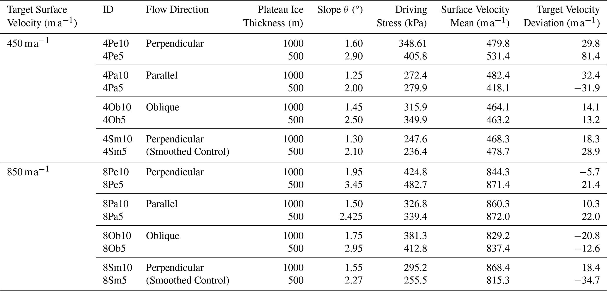
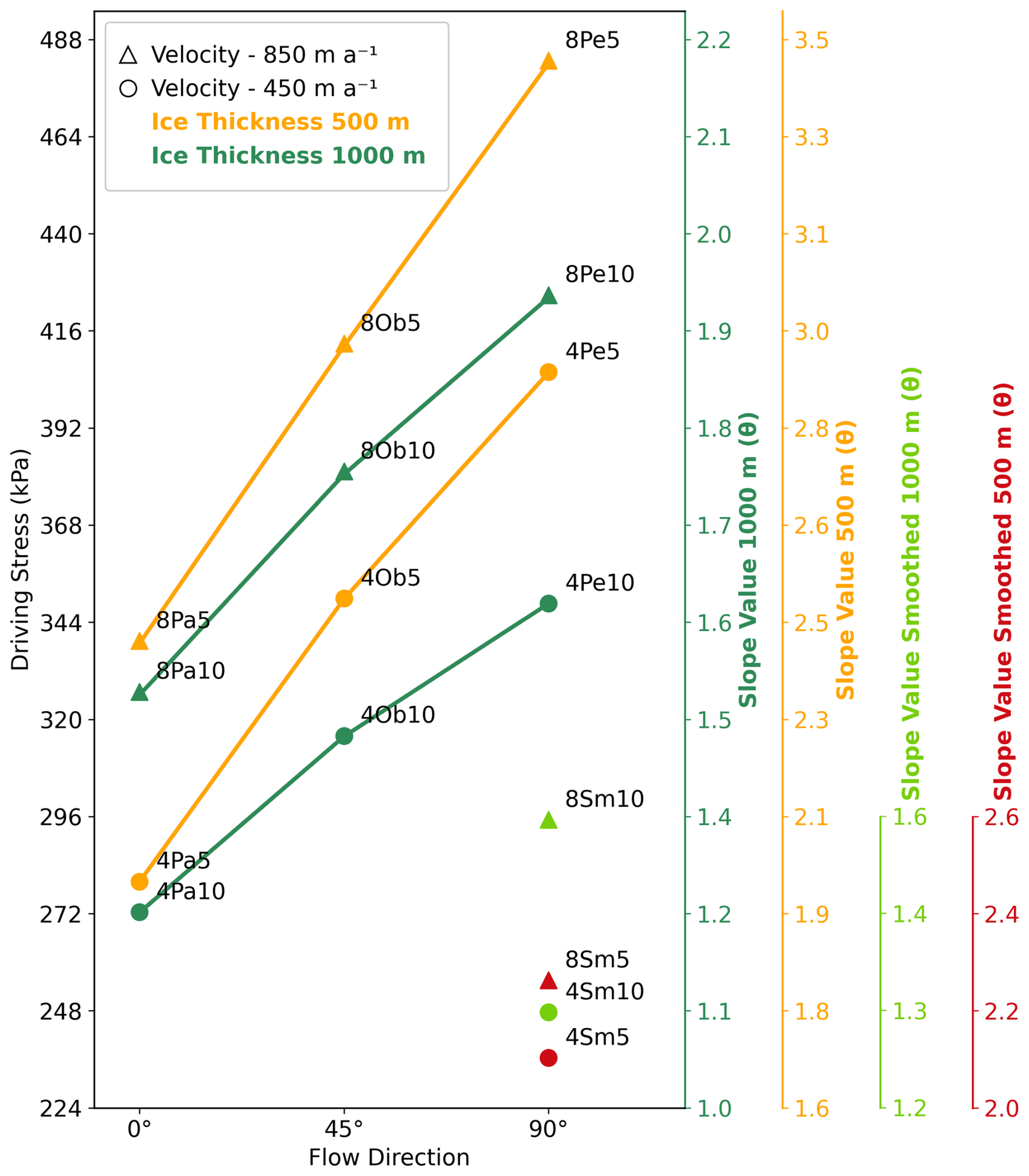
Figure 3 Resulting driving stress values for each selected flow direction, plateau ice thickness and velocity target. Simulations with velocity target of 450 m a⁻¹ are marked with circles, while 850 m a⁻¹ are triangles. Simulations in green have a plateau ice thickness of 1000 m while orange indicates a 500 m thickness. Average ice thickness was used in the driving stress calculation. Smoothed topography simulations have separate ice thickness values (See Sect. 2.1). The label for each marker are individual run IDs corresponding to Table 1.

To reach a target surface velocity, a low fidelity (resolution of 100 m with 10 extruded mesh levels) simulation was used with an ad-hoc approach to tests using increments of 0.05° for θ. The value that produced the closest-to-target average surface velocity (values displayed in Table 1) was then used in subsequent full-resolution simulations. We convert the resulting slope to driving stress for comparison. Driving stress, τ_d, is calculated from domain-averaged ice thickness, H_av, and the slope used to adjust the gravity vector orientation, θ, as

$$\begin{array}{}\text{(12)}& {\displaystyle }{\displaystyle }{\mathit{\tau }}_{\mathrm{d}}=\mathit{\rho }g{H}_{\text{av}}\sin \left(\mathit{\theta }\right).\end{array}$$

The domain-averaged ice thickness, including the fjord hollow, used in τ_d is 1398.6 and 989.6 m for plateau ice thickness values of 1000 and 500 m, respectively. The smoothed control topography DEM yields averages of 1222.6 and 722.6 m for plateau ice thickness 1000 and 500 m respectively.

3 Results

Our results demonstrate the strong control that subglacial fjords and their orientation exert on ice-sheet motion (Fig. 3). For flow-perpendicular simulations, Moffatt eddies and basal flow reversal occurs for both 500 and 1000 m ice thickness above plateau, but only with high-resolution (i.e. not smoothed) topography. Deep perpendicularly-oriented valleys beneath an ice sheet also significantly impede overlying ice motion – comparing one smoothed control simulation (8Sm10, see Table 1) to its high-resolution topography counterpart (8Pe10) yields an increase in slope of 25.8 %, equivalent to a change in area-averaged driving stress from 295.2–424.8 kPa (44 %). Alternative fjord orientations also significantly influence both motion patterns and temperate ice distribution patterns. Here, we cover the following aspects: (Sect. 3.1) perpendicular flow and the associated formation of Moffatt eddies, (Sect. 3.2) parallel flow, and (Sect. 3.3) separation of flow in oblique-orientation simulations. Last, (Sect. 3.4) we compare smoothed-topography control simulations to their high-resolution counterparts.

3.1 Perpendicular flow direction

Across all target velocities and plateau ice thickness combinations for perpendicular flow over high-resolution topography Moffatt eddies (Moffatt, 1964a, b) form at the base of the fjord, accompanied by spiralising lateral ice motion along the lowermost fjord depression. Ice velocity is also greatly affected by the topography. In simulations with target surface velocity of 850 m a⁻¹ (8Pe10), the surface velocity directly above the fjord is ∼120 m a⁻¹ lower than the maximum (Fig. 7d). Absolute velocity within the fjord (below the elevation of the plateau) drops to less than 500 m a⁻¹ (Fig. 4c). This velocity difference creates a distinct shear margin that spans the fjord from crest to crest across the width of the entire domain (Fig. 4). The eddies that form under this shear margin are up to 570 m in diameter. In the case of simulation 8Pe10 with target velocity of 850 m a⁻¹ and plateau ice thickness of 1000 m a secondary set of eddies is also simulated (Fig. 5b).

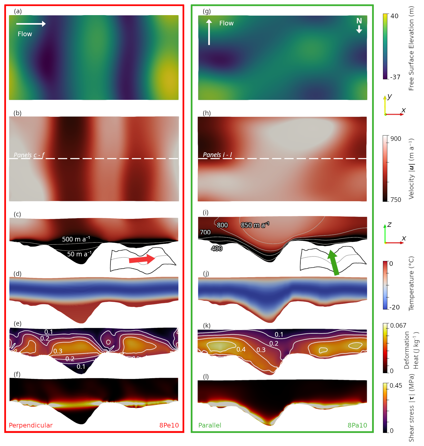
Figure 4 Free surface elevation and velocity of perpendicular 8Pe10 (a–f) and parallel 8Pa10 (g–l) simulations. Panel (a, g) show the free surface elevation, (b, h) show the corresponding surface velocity (m a⁻¹). Panel (c, g) is the velocity field of the cross section from the centre of the domain. Panel (d, h) show temperature (C°) at the same cross section. Panel (e, k) show deformation heat (J kg⁻¹) and panel (f, l) is the shear stress (MPa).

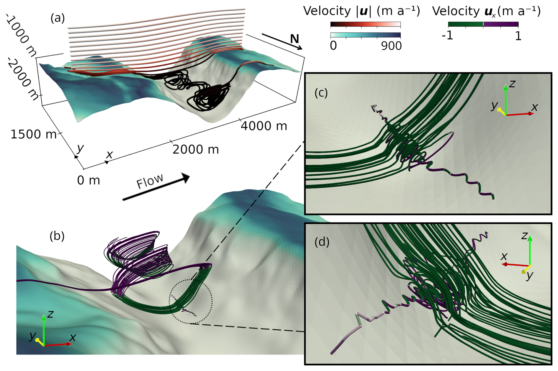
Figure 5 Streamline velocity for perpendicular, 1000 m plateau ice thickness run 8Pe10. Streamlines show that ice from the plateau enters an eddy in the valley, moves laterally, and reappears far to the north on the other side (a). Streamlines of (a) coloured by velocity magnitude. A secondary Moffatt eddy is formed in a small depression in the valley side (b–d). Panel (c) show the larger eddy streamlines flowing from right to left, while the smaller eddy spins counter clockwise in the topographic depression. Panel (d) shows the same secondary Moffatt eddy as in (c) from the opposite side. Streamlines coloured for x direction velocity (b–d), constrained from −1 to 1 m a⁻¹ showing reversal of flow. Target surface velocity 850 m a⁻¹.

Flow from the tributary valley on the upslope plateau, feeds ice flow into the Moffatt eddies. Upon entering the fjord from the tributary, the Moffatt eddy splits laterally, resulting in two independent eddies transporting ice in opposite directions along the fjord. In the free surface runs where periodic lateral boundaries are present (and temperate ice is not) ice is exchanged laterally through the boundary in both positive and negative y orientations, as well as returning back to the main overriding flow. When no-flux boundaries replace lateral periodic boundaries in the thermomechanically coupled runs more ice is directed back into the overriding flow towards the domain edges. The maximum y oriented velocity within the fjord is ∼27 m a⁻¹ (8Pe10).

Just below the margin between the Moffatt eddies in the fjord, and the overflowing ice above, there is a reduction in liquid water content. Partial refreezing of meltwater occurs as the eddies rise on the up-slope fjord side (Fig. 6a.ii). From a Lagrangian viewpoint, the rise increases the pressure melting point and lowers the specific enthalpy at the pressure melting point (H_m(p)) meaning the melt fraction decreases so that the overall specific enthalpy does not change. This temperate ice water content margin is present along the entire valley, following the meeting point between eddy movement and overlying ice (Fig. 6a.i). High stresses and deformation heating between the fjord crests (Fig. 4e,f) results in the formation of a deep temperate layer found in perpendicular simulations (Fig. 6a).

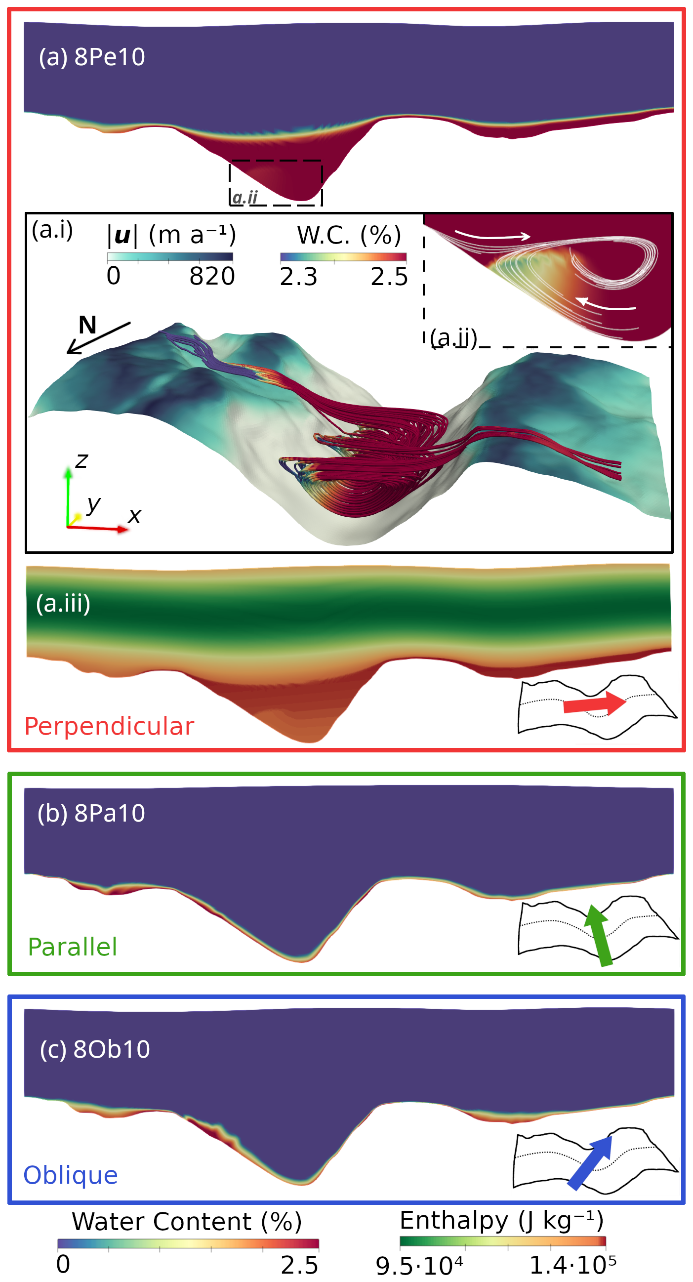
Figure 6 Temperate ice water content comparison of perpendicular (a), parallel (b), and oblique (c) flow direction. Cross sections taken from the centre of the domain. Panel (a.iii) show the enthalpy field of the same cross-section as (a). A change in enthalpy can be spotted along the same margin where the temperate ice water content is reduced in the fjord.

3.2 Parallel flow direction

We use the domain slope and hence domain-averaged driving stress as the main lever to adjust the area-averaged surface velocity. Considering a change in flow direction from parallel to perpendicular over the high-resolution topography with an ice thickness above the plateau of 1000 m, the slope must be altered by 0.45°, corresponding to an increase in averaged driving stress from 326.8 to 424.8 kPa (30 %) (8Pa10 and 8Pe10 respectively). This substantial difference in driving stress between parallel and perpendicular flow indicates the anisotropic nature of a landscapes resistance to flow dependent on its orientation (Fig. 4). The change in slope required to match surface velocity for parallel and perpendicular topography is similar to the difference between actual bed topography and the smoothed control topography (0.40° for simulations 8Pe10, 8Sm10) when both are in the perpendicular orientation (Table 2). The influence of a parallel oriented-fjord on ice surface position and velocity is fairly small, with a much more uniform decrease in velocity with depth when compared to the flow-perpendicular simulations. The temperate ice layer thickness for parallel runs is uniformly much lower than for perpendicular runs, with no large volume of temperate ice occupying the fjord hollow (Fig. 6b).

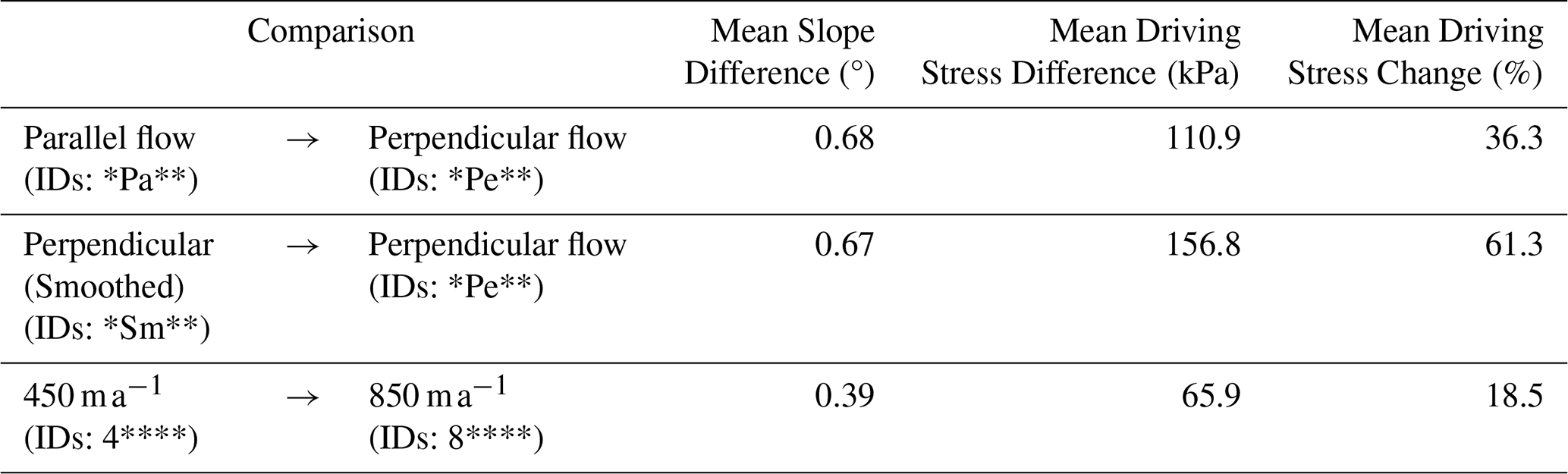
Table 2 Mean slope and driving stress changes for varying simulation comparisons. Taking the average of the differences from all simulation flow directions, plateau ice thicknesses and velocity targets. Smoothed control simulations are excluded from the velocity target comparison and the flow direction comparison.

3.3 Oblique flow direction

In the simulations with oblique flow the flow direction is vertically stratified. At the base of the fjord, the flow aligns with the fjord orientation, while surface flow aligns with the surface slope (Fig. A3). However, surface flow does not directly follow the domain slope (Eq. 3), but deviates from it due to the topographic steering at depth. The simulation with 1000 m plateau ice thickness and target velocity of 450 m a⁻¹ (4Ob10) has a surface flow direction change of 17.1° while the corresponding simulation of 500 m plateau ice thickness (4Ob5) has a surface change of 29.2°. This illustrates how a retreating ice sheet settles into the terrain following flow that results in fjord formation. As with parallel simulations, the thickness of the temperate ice layer is consistently much lower than for perpendicular simulations (Fig. 6c).

3.4 Smoothed control simulation

The perpendicular simulation with 1000 m plateau ice thickness and 850 m a⁻¹ target surface velocity (8Pe10) has an area-averaged driving stress of 424.8 kPa when high-resolution topography is used. In comparison, the smoothed control topography simulation (8Sm10) with equivalent parameters has an area-averaged driving stress of only 295.2 kPa. In this case using a smooth or low fidelity subglacial topography underestimates the driving stress with equivalent average surface velocity by 43.9 %. This effect increases as plateau ice thickness decreases. Comparing the corresponding simulations at 500 m a⁻¹ (8Pe5 and 8Sm5) gives a difference of 227.2 kPa or 88.9 %. On average for all perpendicular simulations, this discrepancy is larger than comparing perpendicular flow to parallel flow at Veafjorden (Table 2).

After decreasing the slope by 0.40°, the smoothed control topography simulation (8Sm10) has a similar surface flow field to the high-resolution topography simulation (8Pe10) (Fig. 7d and h). When comparing local surface velocity over the fjord, both slow down by roughly the same amount. The smoothed control is reduced to 778.1 m a⁻¹ while the high-resolution topography simulation is reduced to 782.3 m a⁻¹. Both reach roughly 920 m a⁻¹ at maximum. Nonetheless, the enthalpy fields, and hence rheological characteristics, between the two settings differ substantially (Fig. 7) with the water content in the control not approaching that of the high-resolution topography simulation. Furthermore, the opening angle (the angle between the two valley sides measured along the flow direction) is much wider in the smoothed control topography (∼169°) than in the high-resolution topography (∼100°), and there is no indication of flow reversal or Moffatt eddies.

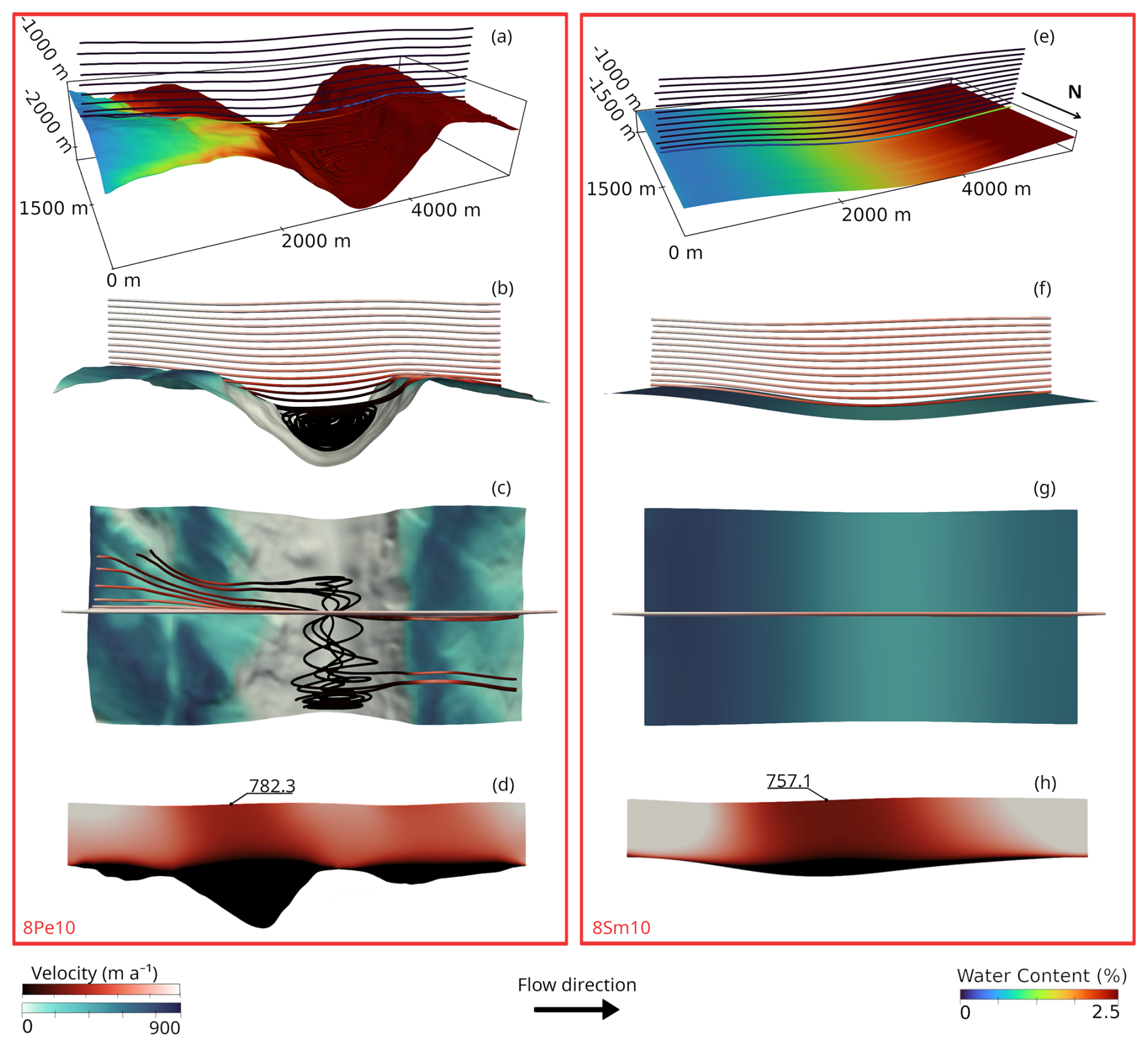
Figure 7 A comparison of Veafjorden perpendicular, 1000 m plateau ice thickness, 850 m a⁻¹ simulation to perpendicular smoothed control. Perpendicular Veafjorden 8Pe10 (a–d). Perpendicular (Smoothed Control) 8Sm10 (e–h). Note that panel (d) and (h) includes tapering region.

4 Discussion

Our results show that realistic fjord geometries – which are common across the margins of the palaeo-Scandinavian ice sheet and also likely across the present day GrIS, yet which are largely excluded from large-scale ice-sheet models – significantly complicate patterns of ice motion and temperate ice. Comparing smoothed control and high-resolution topography simulations, when held at similar surface velocities by adjusting the domain slope, reveals substantially higher driving stresses in the case of high-resolution topography. This is clear evidence for a strong anisotropic response of ice motion to the alignment of the underlying landscape. Moffatt eddies (Gudmundsson, 1997; Meyer and Creyts, 2017) might seem like dramatic and isolated features with limited influence on overall ice-sheet motion. However, our results and analysis of flow-aligned slope angles in western Norway (Fig. 1) suggest that these features are likely widespread in ice motion over incised fjord landscapes.

The complex flow patterns of Moffatt eddies are also dependant on topographic fidelity. The patterns of flow shown in our perpendicular simulations using high-resolution topography (Fig. 5a and b), including eddies and lateral transport along the fjord hollow, closely resemble the 3D simulations in Fig. 9 of Meyer and Creyts (2017). The idealised topography in these simulations invite ascribing a critical angle for Moffatt eddy formation. However, this is complicated somewhat by our use of high-resolution topography which is not well represented by the triangular geometry found in Meyer and Creyts (2017). Nonetheless, an opening angle perpendicular to the fjord of ∼100° is smaller than the critical opening angle α_c=134° for the rheological exponent n=3 in Meyer and Creyts (2017), while the opening angle ∼170° for the smoothed control simulation is above this α_c value. Oblique flow simulations have an opening angle of ∼118°, which would predict the formation of Moffatt eddies. However, no eddies are seen in simulations with these settings. This may be explained by the shift in flow direction exerted by the topography (See Fig. A3d–f) further widening the opening angle. This indicates that a critical value may also have efficacy in predicting Moffatt eddy occurrence in real settings but that low fidelity bed topography products where depressions such as fjords are not resolved are unlikely to be effective indicators of possible Moffatt eddy locations.

Deep fjords furthermore provide a counter-example to suggestions that basal traction should be treated as bounded across all glacier and ice-sheet settings (e.g. Schoof, 2005; Minchew and Joughin, 2020; Zoet and Iverson, 2020; Helanow et al., 2021). In bounded basal traction relationships (i.e. Eq. 11) the traction provided by the bed approaches a maximum value for a given effective pressure that is not exceeded. Whereas, an unbounded basal traction relationship shows a continuous increase in basal shear stress with basal velocity (i.e. Weertman, 1957). For hard beds, the suggestion of bounded basal traction follows from Iken's bound (Iken, 1981; Schoof, 2005), usually expressed as

$$\begin{array}{}\text{(13)}& {\displaystyle }{\displaystyle \frac{{\mathit{\tau }}_{\mathrm{b}}}{N}}\le \text{tan}\left(\mathit{\beta }\right)\end{array}$$

where τ_b is the basal traction and β is the maximum up-slope angle in the mean flow direction. However, Eq. (13) omits traction tangential to the ice-bed interface itself and ceases to become an effective bound in the situation of very steep surfaces (Gagliardini et al., 2007). In the case of ice flow pressing perpendicularly against the near-vertical cliffs present on Veafjorden's western side (Fig. 8), there is no theoretical bound to the resistive traction that could be provided by the cliffs to oppose ice motion. If a large-scale ice-sheet model takes a smoothed basal surface rather than the high-resolution topography, or if the discretisation of the model domain does not permit features such as fjords to be accurately resolved (Fig. 8), then the shear-band features and large slope values included in our high-resolution simulations will create a situation, at least locally, where sliding is not well-described by a bounded sliding relationship limited by Iken's bound with a low value of β. Depending on the exact parameter choice, this could lead to a model grid cell with a defined bounded sliding relationship being unable to provide a physically realistic amount of basal traction for that grid cell. As we hold basal-slip parameters (Eq. 11) constant in both settings, our simulations allow quantification of the influence of fjord geometry on driving stress, showing a significant driving-stress increase is required for the same surface velocity when a high-resolution fjord is used rather than a smoothed representation (Fig. 3).

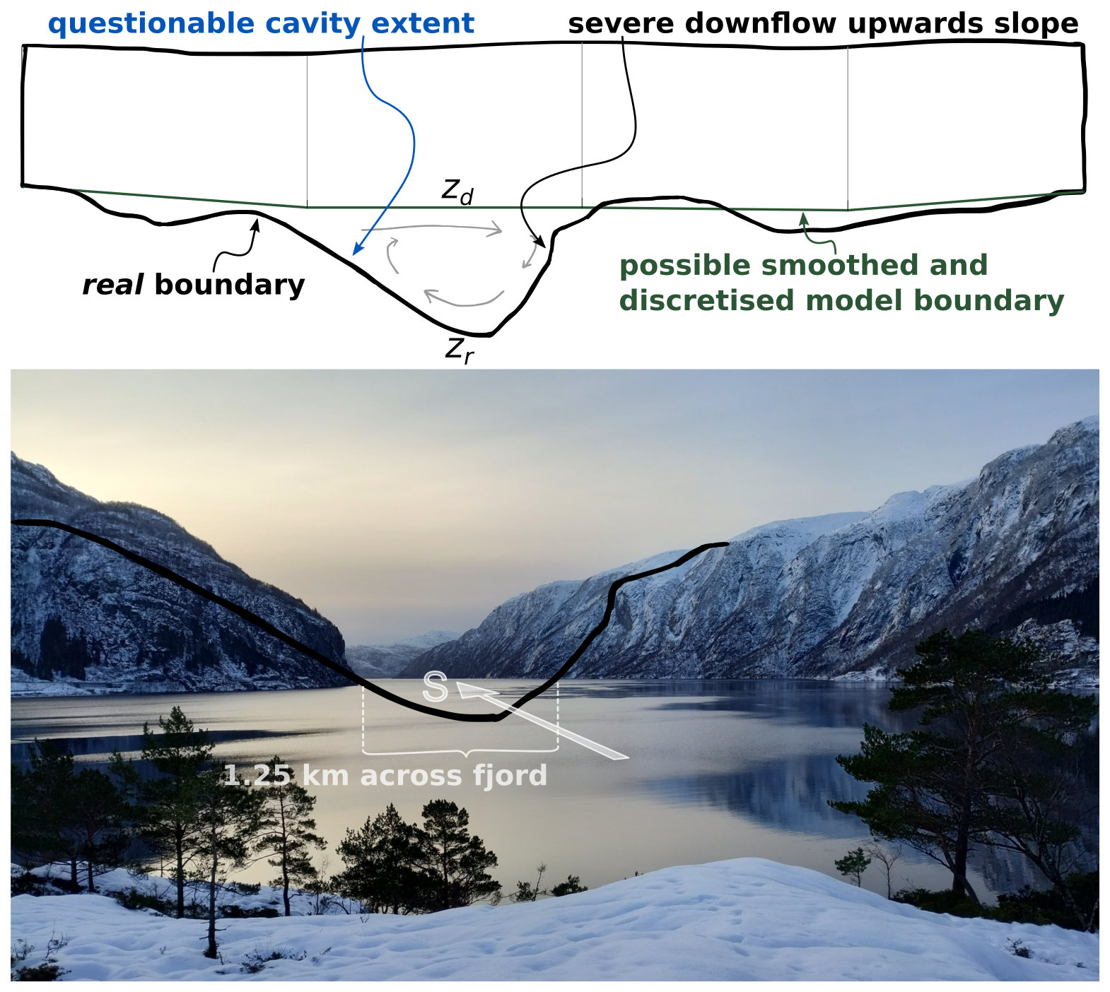
Figure 8 View of vertical cliffs on Veafjorden's western side. z_r and z_d are the high-resolution topography, and a possible discretised representation, respectively. The schematic profile is also traced onto the photo in black. Photo from Sergii Gryshyn taken from Fjordsyn Vaksdal Dagsturhytta.

Classically, cavities may be anticipated to drown out high bed slopes thereby facilitating bounded basal traction (Schoof, 2005; Gagliardini et al., 2007). However, while these studies represent non-dimensionalised problems, their focus is not emphatically on large-scale features such as fjords and the idea of a large cavity within Veafjorden is unintuitive given clear hydrological escape pathways to the north and south (Figs. 1 and 2). Determining the configuration and influence of subglacial cavities in a setting such as Veafjorden should be a focus of future research. Nonetheless, for now we suggest that features such as Veafjorden provide major upslope resistance that is (i) not overcome by cavitation and (ii) not captured by the basal boundary position of ice-sheet models. As the bed slope of cliffs and fjords with flow-aligned slopes exceeding 30° are common across western Norway (Fig. 1) and at least partially representative of the basal topography of the GrIS, we suggest that ice-dynamic interactions with these features provides a physically based background to the utility of unbounded power-law sliding relationships across the GrIS (Maier et al., 2021), which often invoke Weertman sliding (Weertman, 1957), even if the underlying assumptions are not entirely realistic (Weertman, 1979). Given ice sheet responses to changing climate are typically greater for bounded sliding relationships (Tsai et al., 2015), exploring this problem represents an important area for future research.

Ice motion across fjords may also help to explain features revealed in the surface velocity and surface position of the GrIS. Deep fjords exist across the ice-free margins of the GrIS, with the continuation of these fjords inland beneath the ice evident until BedMachine mapping begins to lose its sharpness (Morlighem et al., 2017). Flow-aware hill-shading of the GrIS surface (MacGregor et al., 2024) and analysis of radio-echo flight lines (Paxman et al., 2024) highlight multiple fast-flowing regions where ice flow is inferred to cross subglacial valleys perpendicularly and which appear to align with along-flow surface velocity variations in excess of 100 m a⁻¹ (Fig. A2). This reflects the surface velocity variations modelled in this study (Fig. 4b and c) and indicates a similar topographic control could be at play. Similarly, such a mechanism could be important in East Antarctica where the Aurora Subglacial Basin and Gamburtsev Mountains exhibit multiple subglacial valleys that cross cut the present-day prevailing flow direction (Young et al., 2011; Meyer and Creyts, 2017). Furthermore, basal traction inversions from both the GrIS and AIS evidence complex banded patterns, hypothesised by Sergienko et al. (2014) to result from pattern-forming instabilities in subglacial water pressure. We suggest that they may in fact reflect varying resistance as a result of subglacial topography, indicating the potential influence of large scale topographic obstacles on basal traction fields derived from relatively smooth bed topography products.

Our results also illustrate the anisotropic resistance to ice-motion provided by real subglacial landscapes (Fig. 3), and situations where the basal velocity vector may be non-parallel to its corresponding basal traction vector over a large area (Fig. A3) – previously explored in an idealised case by Hindmarsh (2000). This implies that basal traction patterns should be expected to vary over the lifecycle of an ice sheet, as drainage basins evolve and ice motion patterns shift during growth and decay. Bulk basal motion may furthermore be misaligned with the applied basal shear stress, which could result in complications for dynamic modelling where fine details are important. We leave direct quantification of the influence of landscape anisotropy on basal sliding relationship anisotropy for future work, but recognise that the impact of basal sliding anisotropy is likely small for most predictive timescales (100–1000 yr) in the event that flow orientations do not shift substantially.

Last, geological evidence for the occurrence of the described flow patterns and Moffatt eddies is presently limited to the plateau striations surrounding Veafjorden (Mangerud et al., 2019). These striation markings indicate near-perpendicular flow across the fjord, but do not provide information about the motion within. Reverse direction striations within the valley are possible, but given subsequent ice-flow reorganisations (Mangerud et al., 2019; Reilly, 2023) it is likely that these lineations will have been removed by erosion or overwritten when ice flow switches to follow the fjord orientation.

5 Conclusions

We show that the orientation of fjords relative to the flow direction has a substantial influence on the ice flow magnitude. Significantly greater (∼41 %–89 %) driving stresses are required to push ice perpendicularly over a fjord compared to smoothed control topography, with a clear anisotropic response to fjord orientation apparent. Steep valley walls also present an obstacle not presently resolved in standard ice-sheet model bed products that may result in unbounded, rather than bounded, traction being appropriate and hence explain the efficacy of the power-law sliding relationships across large parts of the GrIS (Maier et al., 2021), which shares basal-topographic similarities with the paleo-Scandinavian Ice Sheet.

At present, it is infeasible and impractical to incorporate this behaviour into large-scale ice-sheet models by increasing resolution and bed-product fidelity. Instead, parameterising the net influence of the behaviour reported here – and that caused by other large-scale topographic obstacles – on basal traction relationships (and basal traction anisotropy) at the more relevant macro scale provides a reasonable pathway for future progress. Doing so may contribute to alleviating uncertainties in predictions of sea level rise (Aschwanden et al., 2021), and to reducing the share of uncertainty in basal traction inversions that pertains directly to sliding processes (Berends et al., 2023).

Appendix A: Calculating flow-aligned hill slope

To quantify the topographic gradient in the direction of surface flow, we computed the flow-aligned gradient using DEM data and flow velocity components. Partial derivatives of elevation in the x- and y directions ($\frac{\mathrm{d}z}{\mathrm{d}x}$ and $\frac{\mathrm{d}z}{\mathrm{d}y}$, hereafter p and q, respectively) were computed from the DEM by fitting a third-order polynomial to a 5×5 window following Florinsky (2017). Flow direction was determined from velocity components v_x and v_y, with velocity magnitude $v_v=\sqrt{v_x^{\mathrm{2}}+v_y^{\mathrm{2}}}$ used to compute unit vectors in the flow direction:

$$\begin{array}{}\text{(A1)}& {\displaystyle }{\displaystyle }\widehat{v}=\left({\displaystyle \frac{v_x}{v_v}},{\displaystyle \frac{v_y}{v_v}}\right)\end{array}$$

The gradients p and q were then projected onto the flow direction by computing the dot product:

$$\begin{array}{}\text{(A2)}& {\displaystyle }{\displaystyle }\text{Flow-Aligned Gradient}=p\cdot {\displaystyle \frac{v_x}{v_v}}+q\cdot {\displaystyle \frac{v_y}{v_v}}\end{array}$$

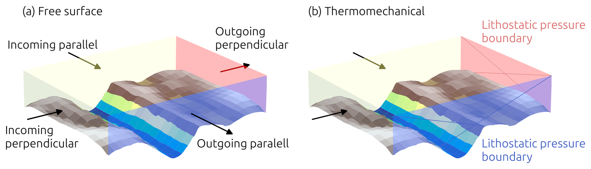
Figure A1 The incoming and outgoing boundaries for the two simulation steps (a) Free surface stage and (b) Thermomechanically coupled stage. Illustrated parallel flow direction and boundary does not represent simulated orientation.

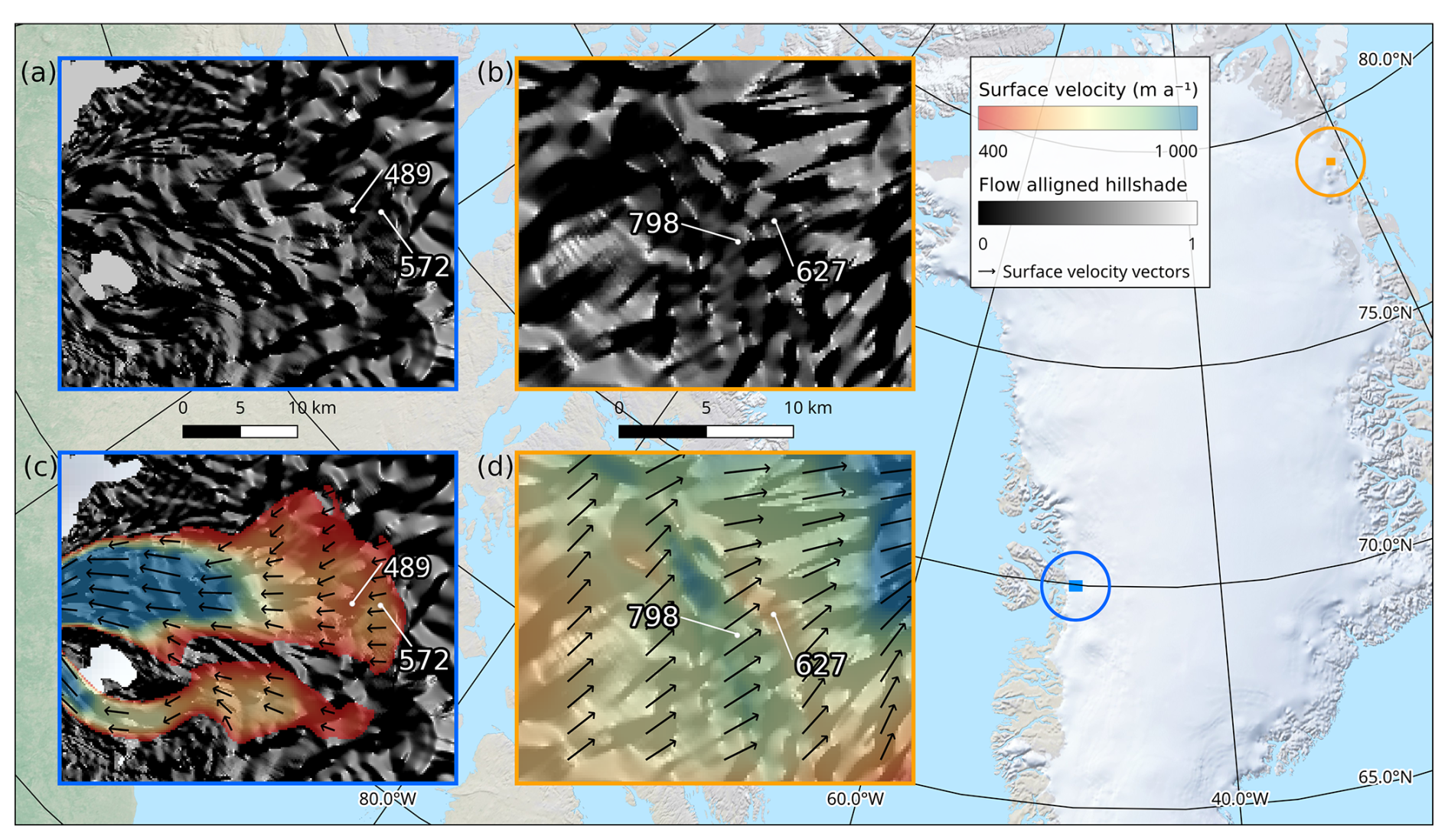
Figure A2 Two example locations in Greenland with variable surface velocity along the same flow line. (a, b) Hill-shade of basal topography with the azimuth computed along the direction of flow (MacGregor et al., 2015). The hill-shade indicate possible areas of subglacial obstacles or valleys. (c, d) Surface velocity data mapped on top of the flow aligned hill-shade in (a) and (b). Several places in the two examples have velocity differences of more than 100 m a⁻¹. Black arrows represent flow direction vectors. Velocity data from Joughin et al. (2010); Joughin (2022); Moon et al. (2023).

The resulting flow-aligned gradient represents the topographic slope in the direction of flow.

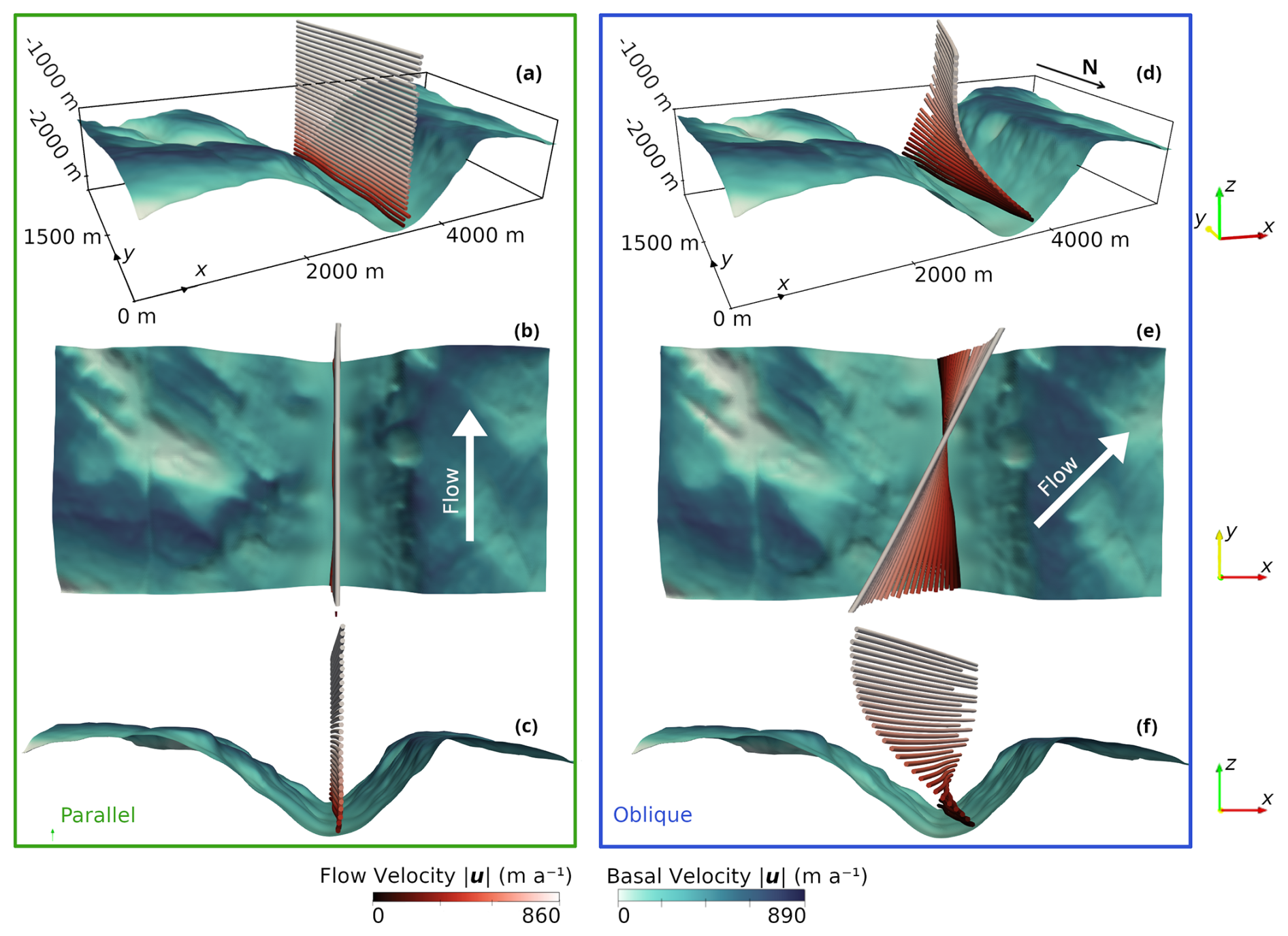
Figure A3 A comparison of parallel flow (a–c) from run 8Pa10, and oblique flow (d–f) from run 8Ob10. Both have a target velocity of 850 m a⁻¹ and plateau ice thickness of 1000 m.

Helanow et al. (2021)Helanow et al. (2021)Gilbert et al. (2014)Gilbert et al. (2014)Cook et al. (2020)Gilbert et al. (2014)Gilbert et al. (2014)Cuffey and Paterson (2010)Duval (1977)

Table A1 Model parameters.