Assessing the potential for an ice core in the southern Antarctic Peninsula to elucidate Holocene climate history

Connecting the West Antarctic Ice Sheet to the southern Antarctic Peninsula, northern Ellsworth Land is a region of enigmatic glacial history now experiencing significant cryospheric change. Large portions of the Bellingshausen-Sea-draining basins have experienced extreme ice thinning and grounding-line change over the satellite observation period. However, the Holocene glacial history of northern Ellsworth Land, which would help to frame the contemporary changes being observed, is poorly constrained. High-resolution ice cores are crucial for reconstructing this past ice-sheet change. We identify a new deep ice-core drilling site at the triple-ice divide point between the Amundsen, Bellingshausen, and Weddell seas (74°34^′37^′′ S, 86°54^′16^′′ W) that could be utilised to address this knowledge gap. Using a transient ice-thinning model, constrained by shallow-ice-core data and dated englacial radar stratigraphy, we estimate records of accumulation and ice thinning, and derive preliminary age-depth scales for the proposed coring site. Inclusion of dated radar stratigraphy in the model improves our constraints on the long-term climate history, and highlights that these data are not compatible with a steady-state assumption. We also show that there has been a significant change in the accumulation rate regime and/or ice thickness throughout the Holocene. A deep ice core at this site would provide a climate record up to ∼ 30 ka with a resolution of 0.58 ka m⁻¹ at 60 m above the ice-bed interface. An analysis of the model sensitivity to basal melting shows that a record beyond the onset of the Holocene could still be recovered under high basal-melt-rate scenarios. We thus conclude that an ice core at this site would yield a valuable high-resolution climate record and provide precise constraints to reconstruct climatic changes and glacial retreat during the Holocene, to help resolve the onset of the extensive dynamic thinning observed today.

1 Introduction

The West Antarctic Ice Sheet (WAIS) is hypothesised to be vulnerable to major collapse with climate warming (Mercer, 1978) and has the potential to contribute several metres to global sea level rise (Edwards et al., 2021; Pritchard et al., 2025). With much of the WAIS grounded in marine basins up to 2000 m below sea level (Lythe and Vaughan, 2001; Fretwell et al., 2013; Morlighem et al., 2017; Pritchard et al., 2025), the area is highly susceptible to mass loss as a result of marine-ice-sheet instability (MISI) induced by ocean warming (Weertman, 1974; Mercer, 1978; Thomas and Bentley, 1978; Pattyn and Morlighem, 2020). Dynamic thinning observed around the ice-sheet margins (Pritchard et al., 2009; Shepherd et al., 2019) has gradually progressed inland (Otosaka et al., 2023), and has motivated several scientific research programmes to investigate whether MISI is underway (Alley et al., 2015; Scambos et al., 2017). The vulnerability of ice to MISI in northern Ellsworth Land, where the WAIS meets the Antarctic Peninsula Ice Sheet (APIS) (Fig. 1), remains poorly constrained and is the focus of this study.

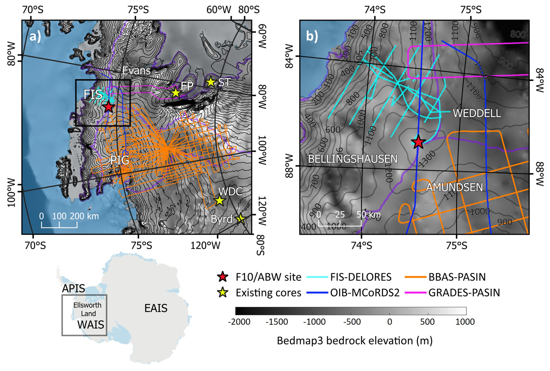
Figure 1 Maps of study area with the datasets and key locations mentioned in this study. (a) Zoom in to northern Ellsworth Land. (b) Zoom in to specific study region. FIS and Evans refer to Ferrigno and Evans Ice Streams, respectively, while PIG refers to Pine Island Glacier. Byrd, WDC (WAIS Divide), FP (Fletcher Promontory), and ST (Skytrain Ice Rise) denote previous deep ice-core drilling sites. The ice divides of the Bellingshausen, Amundsen, and Weddell Sea drainage basins are shown in purple (Zwally et al., 2012), with bedrock elevation data from Pritchard et al. (2025), and CryoSat-2 100 m surface-elevation contours from Helm et al. (2014). Orange, dark blue, light blue and magenta profiles in (a) and (b) show RES profiles; further details for which are outlined in Sect. 2.2.1 and Table 1. The inset below (a) locates the study area. Maps are generated using the Quantarctica mapping environment in QGIS (Matsuoka et al., 2021).

Satellite observations of northern Ellsworth Land have highlighted significant modern ice losses (Wouters et al., 2015; Christie et al., 2016), acceleration (Gardner et al., 2018), and thinning (Shepherd et al., 2019; Nilsson et al., 2022) along the Bellingshausen Sea coastline in recent decades, analogous to the processes observed in the Amundsen Sea Embayment (Turner et al., 2017). Larter et al. (2014) note that current thinning rates are elevated compared to those interpreted from palaeoglacial records (Bentley et al., 2014), but it is unclear whether these contemporary changes are unprecedented during the Holocene due to the large gaps in available data (Jones et al., 2022). Therefore, there is a need to improve our understanding of the vulnerability of ice across northern Ellsworth Land in the face of continued climate warming.

One way to understand better contemporary thinning trends in the context of longer-term change is through ice core analysis (Raynaud and Lebel, 1979). The chemical composition of an ice core can reveal information about the climatic conditions during snowfall deposition (Thomas et al., 2017). Subsequent dating of the ice core through annual layer counting (Sigl et al., 2016; Hoffmann et al., 2022; Emanuelsson et al., 2022), correlation with dated volcanic eruptions (Narcisi et al., 2006; Fujita et al., 2015), comparison of chemical species with other ice cores (Monnin et al., 2004), or ice-flow modelling (Parrenin et al., 2007; Martín et al., 2015; Rowell et al., 2023), can be used to establish an ice-core chronology. These climate records can extend from a few hundred years to thousands of years, and further analyses of the chemical composition of ice layers can give insights into ice-thinning patterns (Raynaud and Lebel, 1979; Grieman et al., 2024), and provide precise constraints for ice-sheet models to reconstruct past ice-sheet configurations (Sutter et al., 2021; Wolff et al., 2025) and infer palaeo-accumulation rates (Martín et al., 2015).

In this paper, we explore the potential for ice at the triple-divide of Pine Island Glacier, Ferrigno Ice Stream and Evans Ice Stream (74°34^′37^′′ S, 86°54^′16^′′ W; Fig. 1) to yield a deep ice core of high resolution suitable for reconstructing Holocene ice and climate history where the WAIS merges with the APIS. As the site also represents the divide between ice draining to the Amundsen, Bellingshausen and Weddell seas, hereafter for convenience we term the proposed ice core location ABW. We first introduce the ABW site, then provide an overview of the radio-echo sounding (RES) and shallow ice-core data that we use to constrain our modelling. We then describe the one-dimensional (1-D) ice-thinning model (Martín et al., 2015; Rowell et al., 2023), and our approach to constraining the model with age observations, to produce a reconstruction of past accumulation and thinning rates throughout the Holocene and into the Last Glacial Period (LGP).

2 Datasets and Methods

2.1 Site Characteristics

The ABW site is situated in northern Ellsworth Land at the intersection of the Amundsen, Bellingshausen, and Weddell ice divides (74°34^′37^′′ S, 86°54^′16^′′ W), where ice is 1220 m deep (Bingham et al., 2012) and ice-surface elevation is 1350 m (Helm et al., 2014) (Fig. 1). The site sits astride a topographic high along the triple-ice-divide on otherwise relatively flat bedrock. Ice flow diverges in three directions away from the divide at a speed of less than 10 m yr⁻¹ (Slater et al., 2024). Shallow ice core data show that surface accumulation rates increased by 27 % between 2000 and 2010 from a previously stable annual average snow accumulation of 33 cm yr⁻¹ before 1900 (Thomas et al., 2015). An automatic weather station was located at the site from December 2009 to December 2010 and showed the monthly average 2 m temperature to range from −15 °C in summer to −30 °C in winter and the annual average wind speed to be around 9.4 m s⁻¹ (Thomas and Bracegirdle, 2014).

2.2 Radiostratigraphy

2.2.1 Radio-echo sounding datasets

We use a combination of airborne and ground-based RES data from several field campaigns throughout West Antarctica between 2004 and 2018. The main surveys include two British Antarctic Survey (BAS) field campaigns that used the Polarimetric Airborne Survey INstrument (PASIN), (1) the 2004/05 BBAS survey over Pine Island Glacier (Vaughan et al., 2006) (hereafter termed “PIG-PASIN”), and (2) the 2006/07 GRADES-IMAGE survey of Evans and Rutford ice streams (Ashmore et al., 2014; Corr, 2021) (hereafter termed “GRADES-PASIN”); an extensive ground-based survey of Ferrigno Ice Stream in 2009/10 (Bingham et al., 2012) using the ground-based BAS DEep-LOoking Radio-Echo Sounder (DELORES; King (2020)); and two profiles from NASA's Operation IceBridge (OIB; MacGregor et al. (2021)) surveys in 2016 and 2018 using the Multichannel Coherent Radar Depth Sounder 2 (MCoRDS2; CReSIS (2024)). Table 1 summarises the relevant information for each RES system. Crucially, each of the RES systems has imaged multiple internal-reflection horizons (IRHs) which act as isochrones across the WAIS (Siegert, 1999). We note that although these RES data were acquired over a period spanning 14 years, modern snow accumulation has been insufficient to induce vertical lowering of internal layers beyond the vertical resolution of each RES system and hence the radiostratigraphies derived from each RES dataset can be considered contemporaneous.

King (2020)Vaughan et al. (2006)Rodriguez-Morales et al. (2014); Arnold et al. (2020)

Table 1 Summary of the three RES systems used in this study.

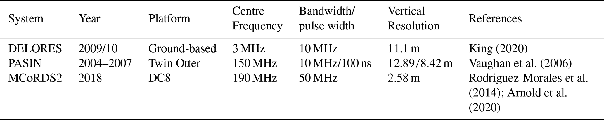
Note: For the PASIN system, we use data from both the chirp- and pulse-acquisition modes and list their individual characteristics in the bandwidth and vertical resolution columns. The vertical resolution for the MCoRDS2 is calculated as per CReSIS (2024) using a scaling factor “k” – see Bodart et al. (2021) for more details.

2.2.2 Tracing internal-reflection horizons

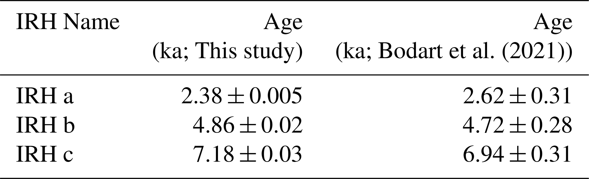
It is now well established that IRHs in Antarctic RES data largely arise from variations in electrical conductivity typically attributed to the deposition of acids from large volcanic eruptions, and hence (with unusual exceptions) can be treated as isochrones (Bingham et al., 2025). The WAIS is home to IRHs that exhibit some of the largest sulphate anomalies of the late Holocene, and these IRHs can be detected and dated precisely and accurately in ice cores (Sigl et al., 2022). Bodart et al. (2021) have previously traced three bright IRHs through the PIG-PASIN dataset across the PIG catchment in West Antarctica, to which they assigned ages of 2.62 ± 0.31, 4.72 ± 0.28 and 6.94 ± 0.31 ka. As these IRHs exhibit such high sulphate anomalies, they can be tied to precise timings of major volcanic eruptions during the Holocene (Cole-Dai et al., 2021), hence here we refine these ages to 2.38 ± 0.005, 4.86 ± 0.02, and 7.18 ± 0.03 ka to correspond to distinctive sulphate peaks in the WD2014 chronology (Buizert et al., 2015; Fudge et al., 2016). Hereafter we will refer to these isochrones as the 2.38, 4.86, and 7.18 ka IRHs. Table 2 clarifies the difference in age assignment between studies.

Bodart et al. (2021)

Table 2 Ages and uncertainties of the IRHs in this study and their respective ages in Bodart et al. (2021).

We traced IRHs through the RES data using Schlumberger Petrel^® 3-D seismic software, applying a semi-automated layer picking algorithm that tracks the local maxima of the received reflections between individual traces. We initiated IRH tracing in the Pine Island Glacier catchment (location A in Figs. 2 and A1), where the traces of Bodart et al. (2021) terminate. Even though the OIB-MCoRDS2 system characteristics differ with the PASIN system (Table 1), these three prominent time markers can also be readily identified in the OIB-MCoRDS2 RES data (Fig. A2), and we thus traced them eastwards along 65 km of a 2018 OIB-MCoRDS2 profile into the Evans Ice Stream catchment (A–A' in Figs. 2 and A1). We then continued to trace the three IRHs along the GRADES-PASIN profile for an additional 68 km until the first intersection with the DELORES survey (A'–B in Fig. 2). This allowed the 2.38 and 4.86 ka IRHs to be extended across large portions of the Ferrigno Ice Stream catchment, and successfully to the ABW site. However, tracing of the 7.18 ka IRH to ABW, and elsewhere across Ferrigno Ice Stream, was disrupted by steeply dipping topography and elevated ice flow (Bingham et al., 2012).

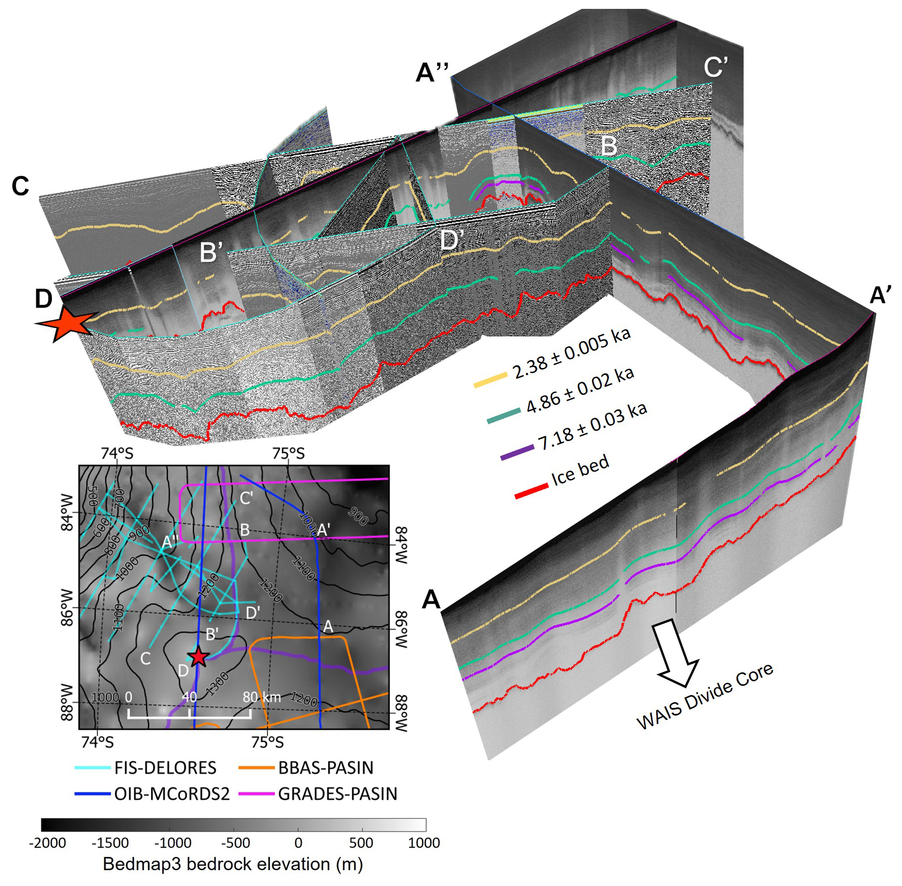
Figure 2 Figure showing a 3-D image of IRHs traced along several intersecting RES profiles from the upper PIG catchment to Ferrigno Ice Stream. RES profiles are orientated looking down Ferrigno Ice Stream towards the Bellingshausen Sea. Inset map (lower left) shows a bird's-eye view of the RES lines in the 3-D image. The red star in both the inset and enlarged figure correspond to the location of ABW. The ice divides of the Bellingshausen, Amundsen, and Weddell Sea drainage basins are shown in purple (Zwally et al., 2012), with bedrock elevation data from Pritchard et al. (2025), and CryoSat-2 100 m surface-elevation contours from Helm et al. (2014).

Appendix A provides detailed information on how each IRH appears across different RES surveys, including key characteristics and uncertainties related to their depths within the ice column.

2.3 Shallow Ice Core Dataset

In December 2010, a 136 m ice core (hereafter termed F10) was drilled at ABW (Thomas et al., 2013, 2015). The F10 core was dated back to 1702, providing a 308-year record of climate variability (Thomas et al., 2013). Snow accumulation was calculated for the entire record using the Nye model (Nye, 1963), and showed a semi-annual cycle, peaking in the autumn and spring (Thomas and Bracegirdle, 2014), with a dramatic increase in accumulation since the onset of the 1900s (Thomas et al., 2015). We use the F10 dataset as a constraint for our inverse model, described in Sect. 2.4.2, to assess the longer-term changes in accumulation rates.

2.4 Model Description

To assess the suitability of a new ice core drilling site, we use a 1-dimensional (1-D) ice flow model, that we will refer to as the forward model, constrained by shallow ice core and dated IRH data to extract surface accumulation records and estimate an age scale for ice at this site. The following section outlines the main principles; Martín et al. (2015) provide the complete numerical derivations.

2.4.1 Forward Model

The age of an ice particle derived from our ice-thinning model is based on the principle that an ice particle deposited on the surface of the ice sheet (of ice thickness, H) is then transported with a velocity ($u,v,w$) through the ice column. As a result, the age of a particle of ice (A) represents the time it takes for a particle of ice to reach a certain position ($x,y,z$), where z represents the vertical component. If we neglect motion from horizontal advection, the age of an ice particle at a specific depth (d) and time (t) can be expressed as a function of the vertical velocity (w), as shown in Eq. (1):

$$\begin{array}{}\text{(1)}& \begin{array}{rl}{\displaystyle \frac{\partial A}{\partial t}}(d,t)& -w(d,t){\displaystyle \frac{\partial A}{\partial d}}(d,t)=\mathrm{1}\mathrm{0}\le d\le H,\\ & -t_{\mathrm{0}}\le t\le \mathrm{0},\\ & A(d,t_{\mathrm{0}})=A_{\mathrm{0}},\\ & A(\mathrm{0},t)=\mathrm{0}.\end{array}\end{array}$$

where A₀ is the initial depth-age, and t₀ is the time before the present t=0. Assuming the time- and depth-dependency of the vertical velocity component of Eq. (1) can be separated, and that there is additionally no basal melting, the vertical velocity is:

$$\begin{array}{}\text{(2)}& w(d,t)=\mathrm{-}\left(a\left(t\right)-{\displaystyle \frac{\partial H}{\partial t}}\right){\displaystyle \frac{{\mathit{\rho }}_i}{\mathit{\rho }\left(d\right)}}\mathit{\eta }\left(d\right),\end{array}$$

where a is the time-dependent surface accumulation rate, ρ is density, ρ_i is the density of ice, and η(d) is the shape function. For simplicity, we initially assume that there are no changes in ice thickness over time $\left(\frac{\partial H}{\partial t}=\mathrm{0}\right)$ and we discuss the implications of this assumption in Sect. 4.1. Numerically, we solve Eq. (1) using a semi-Lagrangian, two-time level, method (Staniforth and Côté, 1991).

As the precise ice-flow conditions at ABW are unknown, we initially use two extreme approximations for the shape function, (1) the Lliboutry approximation (see Eq. 3; Lliboutry (1979)) useful for simulating ice thinning at the “flanks” of the ice flow divide, and reproducing ice flow dominated by shear (Martín and Gudmundsson, 2012); and (2) an approximation for representing ice flow at the “divide” from Martín and Gudmundsson (2012).

$$\begin{array}{}\text{(3)}& \mathit{\eta }\left(d\right)=\mathrm{1}-{\displaystyle \frac{p+\mathrm{2}}{p+\mathrm{1}}}\left({\displaystyle \frac{d}{H}}\right)+{\displaystyle \frac{\mathrm{1}}{p+\mathrm{1}}}{\left({\displaystyle \frac{d}{H}}\right)}^{p+\mathrm{2}},\end{array}$$

The Lliboutry parameter p in Eq. (3) affects the non-linearity of the vertical velocity (Lilien et al., 2021); a higher p implies more deformation in the vertical component, and is used to describe the vertical velocity w in different “flank” flow regimes. Assumptions associated with the vertical velocity profile include that ice is isotropic, and that bedrock variations are smooth.

Our initial model solutions assume that the accumulation rate changes are proportional to the WAIS Divide record (Buizert et al., 2015; Fudge et al., 2016), and we use the advection-corrected accumulation rate from Koutnik et al. (2016), which extends to ∼ 31 ka. As we do not know the precise long-term ice flow conditions at ABW, we hypothesise that ice flow at this point is bounded by both extreme approximations, and so we run the forward models for both “flank” and “divide” ice-flow regimes.

2.4.2 Inverse Model and Optimisation Routines

To date the entire ice column, we formulate an inverse problem of the forward model that assimilates age observations from F10 shallow ice core data (Thomas et al., 2013, 2015) and new dated radar stratigraphy (Sect. 2.2.2). This approach seeks the optimal records of the accumulation history and ice thinning $\left(a\left(t\right)-\frac{\partial H}{\partial t}\right)$ that minimise the difference between the observed age markers and the modelled age-depth profile (Martín et al., 2015). As we initially assume that there are no changes in ice thickness through time $\left(\frac{\partial H}{\partial t}=\mathrm{0}\right)$, our inversion combines changes in ice thickness with the accumulation history a(t).

To estimate the accumulation rate history between observed time markers, we assume a set of initial solutions for the surface accumulation at ABW that are derived from both the F10 core and IRH data, and then we assume that a(t) is a piecewise linear function and vary the Lliboutry parameter p from 1 to 5 to simulate ice flow at the “flanks”. Beyond the deepest observed time marker (a 4.86 ka IRH at 874.1 m), we assume the accumulation rate is proportional to that of the WAIS Divide Ice Core (Buizert et al., 2015; Fudge et al., 2016), and scale the modern accumulation rate estimates from annual layer counting (Thomas et al., 2015) appropriately.

For the optimisation, seeking the piecewise accumulation history that better fits observations, we use a simplex method from Lagarias et al. (1998), as coded in the MATLAB fminsearch function. To avoid over-fitting to the observed F10 and IRH data, we add a regularisation term proportional to the temporal gradient of accumulation $\left(\frac{\partial a}{\partial t}\right)$ to the difference between observations and model. We perform L-curve analyses to determine an optimal regularisation parameter (Fig. B2) (Hansen, 2001; Wolovick et al., 2023). Small values of the regularisation parameter lead to over-fitting with extreme variations in a(t), while large values of the parameter smooth out any fluctuations in a(t). We then choose an optimal regularisation parameter such that the solution lies between these two extremes (the corner of the L-curve), and derive this mathematically through curvature analysis (Appendix B2) (Wolovick et al., 2023).

Using this optimised accumulation history, we derive an age scale at ABW with Eq. (1), which forms Scenario 1 in Table 3.

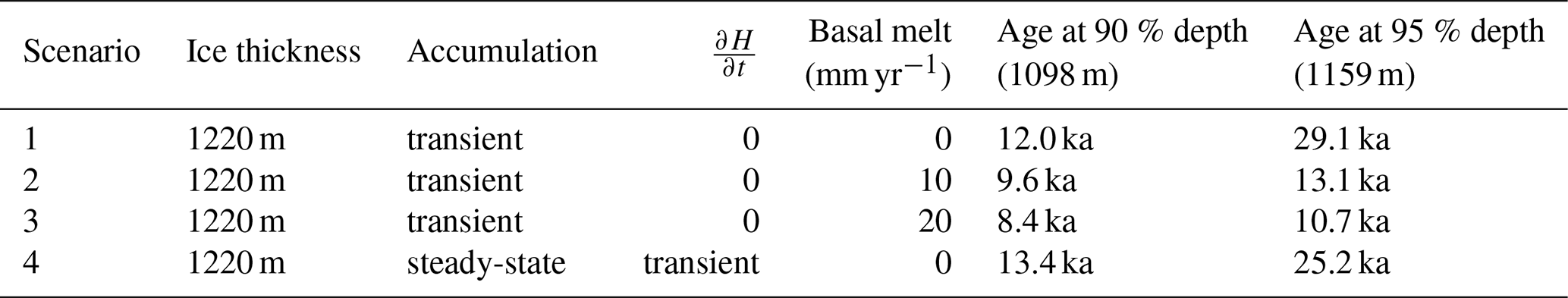
Table 3 Outline of our four inverse model scenarios at ABW and the ice age estimates at 90 % and 95 % of the ice thickness for each optimisation.

2.4.3 Sensitivity to Basal Melting

Our initial optimised solutions are based on the assumption of no basal melting to assess the maximum possible ice record that could be recovered at ABW. We assess the sensitivity of our model to basal melting to thoroughly investigate the suitability of the proposed ice core site.

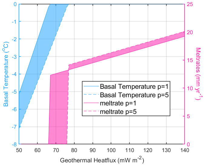
To do this, we initially used a 1-D steady-state temperature model (Jordan et al., 2018) that, similar to Eq. (1), derives the ice temperature at a given depth and time as a function of the vertical velocity. The model is constrained by ice thickness (1220 m), surface temperature (−20 °C) (Thomas and Bracegirdle, 2014), modern accumulation rates (0.33 m yr⁻¹) (Thomas et al., 2015), and various geothermal heat flux (GHF) values to calculate a range of basal temperatures. As the GHF across West Antarctica is so poorly constrained (Burton-Johnson et al., 2020; Hazzard and Richards, 2024) and the precise basal conditions at the site are unknown, we ran the temperature model across a wide range of unknown GHF values (50–140 mW m⁻²) to account for different basal melt regimes. Burton-Johnson et al. (2020) calculated the maximum mean GHF of five continent-scale geophysical estimates to be 106 mW m⁻² and thus our range of modelled GHF accounts for variations between continent-scale estimates of GHF and their uncertainties.

Under these initial boundary conditions, the model indicates that there will be melting at the bed if the GHF exceeds 67 mW m⁻² as this is when the basal temperature exceeds 0 °C (Fig. C1). A detailed breakdown of the steady-state temperature model can be found in Jordan et al. (2018).

Using the values from these simulations, we quantify the basal melting m (Leysinger Vieli et al., 2018) using the following equation:

$$\begin{array}{}\text{(4)}& m={\displaystyle \frac{Q_{\mathrm{G}}(x,y)-k_{\mathrm{c}}\frac{\partial T(x,y,d,t)}{\partial d}{|}_{d=\mathrm{0}}}{{\mathit{\rho }}_{w}L}}\end{array}$$

where Q_G is the geothermal heat flux, k_c is the thermal conductivity, L is the latent heat, and ρ_w is the density of water. This calculation of basal melting neglects contributions of heat generated by sliding (horizontal surface velocity is low) and subglacial water flow, and so it is reasonable to assume that GHF would be the largest contributor to melting at the ABW site.

Using Eq. (4), we calculate the melt rates at ABW to range from around 10 to 20 mm yr⁻¹ for different input GHF values (highest GHF =140 mW m⁻²). We then incorporate these melt rates into Eq. (2) to assess the sensitivity of the original age-depth solution (Scenario 1) to basal melting. These scenarios correspond to Scenarios 2 and 3 in Table 3.

2.4.4 Constraining thinning history at ABW

Our initial scenarios assume that there have been no changes in ice thickness over time (Eq. 2: $\frac{\partial H}{\partial t}=\mathrm{0}$) and that changes in the vertical velocity component are entirely influenced by changes in the accumulation regime (a(t)) at ABW. To study the implications of a variable ice thickness, we introduce a normalised elevation term, $\mathit{\zeta }(d,t)=d/H\left(t\right)$ (similar to King et al. (2025)) and, using the chain rule of derivatives, rewrite our age-depth equation (Eq. 1) as:

$$\begin{array}{}\text{(5)}& \begin{array}{rl}& {\displaystyle \frac{\partial A}{\partial t}}+(\dot{a}\mathit{\eta }+\dot{H}\mathit{\zeta }){\displaystyle \frac{\mathrm{1}}{H}}{\displaystyle \frac{\partial A}{\partial \mathit{\zeta }}}=\mathrm{1},\\ & A(\mathrm{0},t)=\mathrm{0}-t_{\mathrm{0}}\le t\le \mathrm{0},\\ & A(\mathit{\zeta },t_{\mathrm{0}})=A_{\mathrm{0}}\left(\mathit{\zeta }\right)\mathrm{0}\le \mathit{\zeta }\le \mathrm{1}.\end{array}\end{array}$$

where $\dot{a}$ represents the accumulation rate history, a(t), and $\dot{H}$ is the time derivative of the ice thickness, $\frac{\partial H}{\partial t}$.

To estimate the ice thickness history between observed time markers, we assume an initial set of thinning rates at our time markers, and then follow a similar procedure to Sect. 2.4.2 and assume that $\dot{H}$ is a piecewise linear function between time markers. Beyond our deepest time marker (4.86 ka) we assume there are no changes in ice thickness, $\frac{\partial H}{\partial t}=\mathrm{0}$. To simplify the model, we also assume that the accumulation, a(t), has been in steady-state (constant over time) and that the changes in ice thickness are much smaller than the initial ice thickness $\left(\frac{\partial H}{\partial t}\ll H_o\right)$. We then optimise the model to seek a piecewise ice thickness history that best fits our age observations and reveals periods of thickening or thinning at ABW through the Holocene. This will be referred to as Scenario 4. Table 3 provides summaries of each of our four modelled scenarios at ABW.

3 Results

3.1 Geophysical observations

Previous work using the ground-based DELORES survey data identified the presence of a deep subglacial trough running along the centre of Ferrigno Ice Stream (Bingham et al., 2012). The DELORES survey also follows the ice divide and images continuous IRHs and a relatively flat ice-bed interface at the ABW site. The bedrock relief away from the dome at ABW is around 700 m. Coherent layers are imaged in the DELORES data at ABW to around 1080 m depth, approximately 89 % of the total ice thickness (1220 m), with layers tending to conform to the bed topography. Although we could only trace two dated IRHs to ABW, there are other traceable layers present above and below the 4.86 ka IRH which, with additional age-depth constraints, could be dated. The elevated accumulation rates at ABW, relative to more inland sites, are likely to produce well-defined annual layers (Palmer et al., 2001) that are effectively imaged by RES, and would provide high-resolution layers within ice-core data.

Mutter and Holschuh (2025) analysed RES data alongside ice-core data at 16 ice-core sites, noting that locations with laterally continuous layers imaged to significant depths in the RES data often provided the most continuous climate records, while sites with larger sections of incoherent scattering were often associated with more disturbed ice-core records. In the DELORES data at ABW, continuous layering is present to 89 % depth with a small region of absent layering, suggesting promising drilling conditions that could allow the recovery of a continuous and undisturbed climate record.

3.2 Accumulation rate history and ice thinning

Figure 3 shows the reconstructed accumulation rates for Scenario 1 derived from the inverse model in Sect. 2.4.2 which assumes $\frac{\partial H}{\partial t}=\mathrm{0}$. We include accumulation rate data from the WAIS Divide (Buizert et al., 2015; Fudge et al., 2016) and Dome C (Parrenin et al., 2007) ice cores alongside for comparison and to place the ABW site in the context of other deep ice cores across the Antarctic Ice Sheet. We indicate on Fig. 3 which regions of the solution are constrained by age-depth observations from the F10 core and dated-IRHs, and which regions are scaled to the WAIS Divide accumulation rate record.

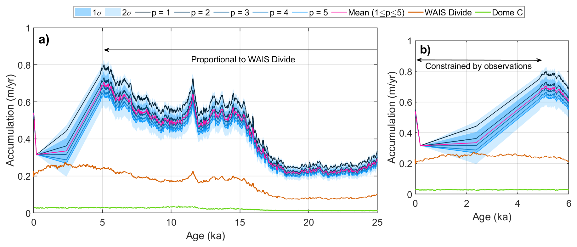
Figure 3 Modelled accumulation rates at the ABW core for different “flank” flow regimes ($\mathrm{1}\le p\le \mathrm{5}$). Pink line represents the mean across all simulations, orange and green lines correspond to the accumulation records from the WAIS Divide (Buizert et al., 2015; Fudge et al., 2016) and Dome C (Parrenin et al., 2007) ice cores, respectively, and are included on both panels for reference and comparisons in the manuscript. (a) Accumulation rate reconstruction to 25 ka from Scenario 1, (b) shows the period where our simulations are constrained by only F10 and dated-IRH observations.

There is a peak accumulation rate of ∼ 0.7 m yr⁻¹ around 5 ka. The magnitude of this peak accumulation is around 20-30 % higher than the modern accumulation rate estimates from the F10 shallow-ice-core data (Thomas et al., 2015). Comparisons with the WAIS Divide record suggest that the accumulation rates at ABW could be up to three times those measured at WAIS Divide (Fig. 3).

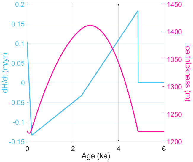
Figure 4 Modelled rates of ice thickness change and estimates of ice thickness evolution at the ABW site from Scenario 4 over the period where our simulations are constrained by F10 and dated-IRH observations.

Figure 4 shows the optimised history of the rate of change of ice thickness at ABW from Scenario 4, and the integrated history of ice thickness from solutions to Eq. (5). Here we see around a 200 m drop in ice thickness since 2.38 ka to the present-day ice thickness (1220 m). Initially, we ignored changes in ice thickness (Fig. 3); here, we assume that accumulation has been in a steady-state and that there were no changes in ice thickness beyond 4.86 ka (Fig. 4). Neither of these assumptions is perfect, but they together give a better indication of what may have happened at ABW since the onset of the Holocene. In reality, the accumulation regime has not been in steady-state and the ice thickness has likely evolved constantly; however, the results of Figs. 3 and 4 show that there have been significant changes at ABW during the Holocene, which is an exciting prospect for ice-core drilling.

3.3 Ice age-depth scale

Figure 5 shows the modelled age-depth profiles, with associated uncertainties, for the proposed ABW ice core for different basal melt rate and thinning scenarios (Table 3). For our scenarios that do not consider the effects of basal melting (Scenarios 1 and 4), predicting the age of the ice close to the ice-bed interface is uncertain since the solution to Eq. (1) tends to infinity (Fig. 5). Furthermore, the model outputs in the deepest parts of the ice column become unrealistic due to their dependence on input parameters. As a result, for all scenarios we take a conservative estimate of the age of the oldest ice at 95 % depth (1159 m; around 60 m above the ice-bed interface; see Table 3).

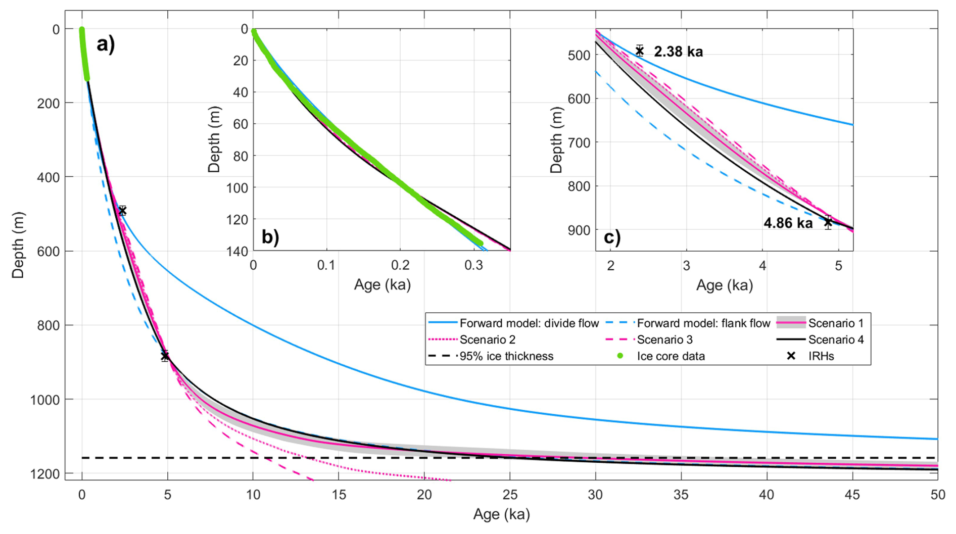
Figure 5 Age-depth profiles from initial forward models and four inverse model scenarios. Scenario 1 corresponds to transient accumulation and no ice thickness changes or basal melting, Scenarios 2 and 3 introduce 10 and 20 mm yr⁻¹ basal melting, respectively, and Scenario 4 models ice thickness changes with steady-state accumulation and no basal melting. Grey shading around Scenario 1 indicates the uncertainty between different flank flow regimes ($\mathrm{1}\le p\le \mathrm{5}$). Age-depth constraints from F10 shallow ice core data are shown in green, and black crosses indicate the dated-IRHs, with error bars placed on the IRH time markers corresponding to the depth and age uncertainty in these tracings. The dashed black line marks 95 % ice thickness where we infer the age of the oldest ice at ABW. (a) Age-depth profiles up to 50 ka, (b) zoomed-in age-depth profiles for the period observed with shallow ice core data, (c) zoomed-in age-depth profiles for the dated-IRH period.

Our results at this depth for Scenario 1 (solid pink line in Fig. 5), imply that ice ages may be older than the Last Glacial Maximum (Clark et al., 2009), spanning between 22.1 and 38.4 ka for different flank flow scenarios. The oldest ice averaged across all “flank” flow simulations at this depth is 29.1 ka. Incorporating thinning into the model in Scenario 4 decreases the age of the deepest ice, but still suggests the recovery of ice up to 25.2 ka at 95 % of the ice thickness (Table 3).

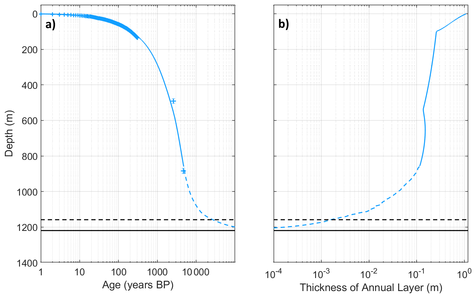
Figure 6 Age and annual layer thickness depth profiles at the ABW site. (a) Optimised age-depth profile from Scenario 1 on Fig. 5 on a log scale. Blue crosses indicate age observations used to constrain the inverse model. (b) Annual layer thickness estimates from the inverse model output. In (a) and (b) blue solid lines indicates where the profiles are constrained by age observations (blue crosses; F10 age data and dated-IRHs), with the dashed blue lines corresponding to where the profiles are constrained by WAIS Divide accumulation data (Buizert et al., 2015; Fudge et al., 2016). Solid and dashed black lines in both panels represent the ice thickness and 95 % depth, respectively, at the ABW site.

Figure 6 shows the resolution and layer thickness of the ABW ice core. Assuming that annual layers can be resolved down to the centimetre scale (Hoffmann et al., 2022; Grieman et al., 2022), the model output suggests that annual layers at ABW could be resolved beyond 7 ka. Additionally, at 95 % of the ice thickness, the resolution is ∼ 0.64 ka m⁻¹, suggesting that the ice at this depth could be both high resolution and highly resolvable, potentially containing a climate record that extends well into the LGP.

3.4 Sensitivity to basal melting

Incorporating basal melting into model simulations results in greater drawdown of layers in the lowest third of the ice column (Jordan et al., 2018) and, in turn, the age-scale becomes more linear (Fig. 5). This reduces the estimated retrievable climate records, at 95 % ice thickness, to 13.1 and 10.7 ka under moderate (10 mm yr⁻¹: 67 mW m⁻²) and extremely high (20 mm yr⁻¹: 140 mW m⁻²) GHF scenarios (Fig. 5 and Table 3). These melt rates are likely overestimated by derivations from an overestimate of the true GHF at ABW. This will in turn underestimate the oldest ice at ABW and hence we treat these simulations as “worse-case” scenarios for basal melting at ABW. Regardless of the actual basal melting values, the results from Scenarios 2 and 3 show that a climate record extending beyond the Holocene could still be recovered even if there was some melting at the ice-bed interface.

3.5 Age-depth along the ice divide

Figure 7 displays the modelled age outputs at 95 % ice thickness at ∼ 350 m intervals along the ice divide separating Ferrigno Ice Stream from Pine Island Glacier and Evans Ice Stream. These outputs assume that (1) modern accumulation rates are identical to those at the ABW site (Thomas et al., 2015), (2) flank flow conditions (p=3) to account for divergence of the RES traverse from the true divide, and (3) no basal melting. The model is then optimised using new ice thickness and dated-IRHs at intervals along the DELORES divide traverse in Fig. 2. In general, we observe older ice in regions of deeper bed topography, but the thickest regions of the divide do not always exhibit the oldest ice (see central divide region of Fig. 7). Regions with relatively low ice thickness and older ice, such as the ABW site, would be more optimal for ice core drilling.

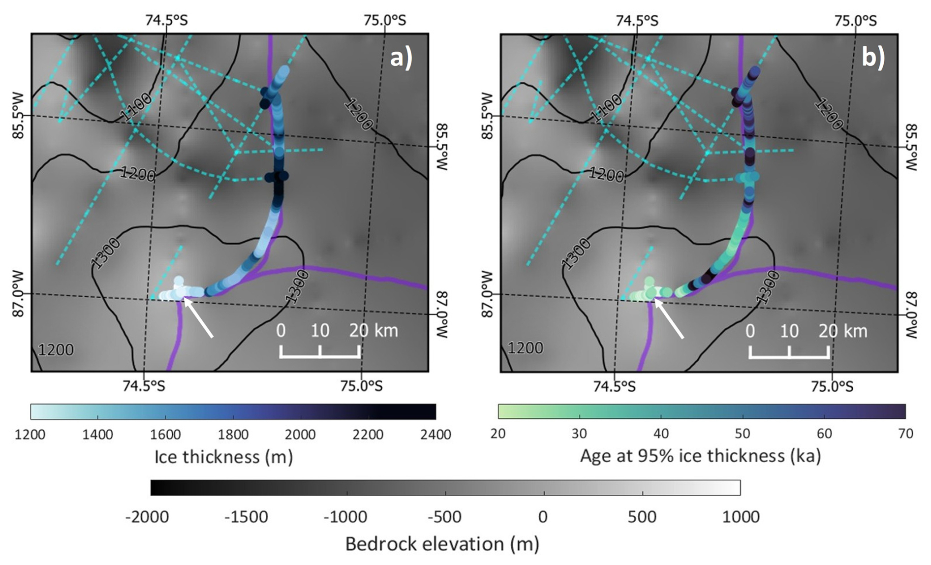
Figure 7 (a) Ice thickness derived from the bed picked in DELORES data, and (b) modelled age of ice at 95 % ice thickness. In both panels: arrow indicates location of ABW, dashed cyan lines represent the DELORES traverse, purple lines outline drainage basin from Zwally et al. (2012), black lines indicate surface elevation contour data from Helm et al. (2014), and data are overlaid on top of bedrock elevation data from Pritchard et al. (2025).

The results of modelling along the DELORES divide traverse highlight the possibility of recovering older ice at locations that offer a thicker ice column. However, comparing the modelled age to the drill depth (ice thickness) suggests that the ABW site offers a valuable climate record for its relatively low drill depth. This makes the ABW site attractive, logistically and financially, as it captures a comprehensive Holocene climate record while minimising drilling time and/or costs, and hence the subsequent environmental impact.

4 Discussion

4.1 Holocene ice thinning

One of the goals of drilling a deep ice core at ABW is to recover a record of ice that can provide information on the onset of ice thinning through the Holocene.

Our initial scenarios (1–3) assume constant ice thickness at the site $(\frac{\partial H}{\partial t}=\mathrm{0}$ in Eq. 2). As a consequence, our model interprets an increase in ice thickness as an increase in accumulation. This is because the ice particles travel faster to their present locations as the ice thickness increases and, with the assumption of constant geometry, the increase in speed is inverted as an increase in accumulation. This raises the question whether the observed changes in accumulation reconstruction (Fig. 3) are the result of changes in surface accumulation, ice thinning, or a combination of both, as our initial model scenarios cannot differentiate between them. Although recent changes at ABW have been interpreted as a result of a recent increase in accumulation (Thomas et al., 2015), there have also been reports of ice thinning in the Weddell Sea sector (Grieman et al., 2024) and even re-advance and thickening around the Ross Ice Shelf area (Kingslake et al., 2018) during the Holocene (Jones et al., 2022). In an area currently experiencing significant changes in ice mass and ice-thinning in the contemporary period (Wouters et al., 2015; Christie et al., 2016; Shepherd et al., 2019; Nilsson et al., 2022), the ABW site, which lies in the coastal area adjacent to the Bellingshausen and Amundsen Seas, is particularly important for reconstructing climatic changes and glacial retreat during the Holocene, and addressing the uncertainties surrounding whether the interior WAIS is thinning or thickening.

In an attempt to understand the thickness history at ABW in more detail, we introduce a normalised elevation term into our age-depth model (Sect. 2.4.4). Including this scenario (4) allows for a quantitative estimate of thickness changes at ABW since 4.86 ka, and gives an indication of the magnitude of thickness changes at ABW over this period. As observed with previous scenarios (Fig. 3), Fig. 4 indicates significant changes at ABW between 4.86 ka and present-day. The thickening observed between 4.86 ka and 2.38 ka in Fig. 4 is the result of assuming $\frac{\partial H}{\partial t}=\mathrm{0}$ beyond 4.86 ka. Furthermore, the model initially underestimates the ice thickness at ABW before 4.86 ka, which leads to an instantaneous increase in the rates of thickness change at this time marker, causing a drastic change in ice thickness as the model compensates for the initial underestimation. Where the solution is constrained by time markers, we observe over 200 m of thinning between 2.38 ka and present-day, as ABW transitions from a thickening to thinning regime. This magnitude of Holocene ice thinning is consistent with other studies in West Antarctica (Hein et al., 2016; Grieman et al., 2024), but we cannot precisely pinpoint the timing of this transition due to the temporal discontinuities between our limited time markers. Additionally, the absence of current constraints beyond 4.86 ka means that we cannot resolve the history of ice thickness from the mid-to-late Holocene, a period over which both thinning (Grieman et al., 2024) and thickening (Kingslake et al., 2018) have been observed in West Antarctica. An ice core at ABW would help to resolve these uncertainties and improve our understanding of the state of the interior WAIS during the Holocene.

Our reconstructions in Fig. 3 also show elevated accumulation relative to other more inland ice cores in West Antarctica (Buizert et al., 2015; Fudge et al., 2016), which implies that the ice recovered could have high resolution and highly resolvable layers (Palmer et al., 2001). Combining this with the drastic change observed between 5–2 ka makes this site attractive for ice-core drilling as the model for each scenario suggests a significant change occurred during the mid-Holocene at ABW. In West Antarctica, both elevated accumulation rates using radar stratigraphy (Siegert and Payne, 2004; Neumann et al., 2008; Karlsson et al., 2014; Fudge et al., 2016; Koutnik et al., 2016; Bodart et al., 2023) and ice thinning signals from geomorphological, cosmogenic nuclide, and ice-core data (Hein et al., 2016; Grieman et al., 2024) have been observed since the mid-Holocene. Given the magnitude of the observed decrease in accumulation in Fig. 3 and the changes in ice thickness observed in Fig. 4, it can be inferred that this signal in the model output was likely caused by a combination of both extensive ice thinning and a change in the accumulation regime at ABW.

To resolve climatic changes accurately at ABW, and confirm the signal as an ice-thinning, accumulation rate decrease, or somewhere in between, we need an ice core. Recent work by Grieman et al. (2024) at Skytrain Ice Rise demonstrated the ability to resolve similar signals using ice-core data. In their study, they identified a 450 m ice-sheet thinning signal between 8.2 and 8.0 ka and substantial retreat of the ice front between 7.7 and 7.3 ka due to ice-flow changes induced by ungrounding. The maximum modelled change in ice thickness at ABW between 4.86 and 2.38 ka, if we assume that the accumulation rate has remained constant, is around 250 m. This suggests that the order of magnitude of the potential ice thinning estimated by the model at ABW is consistent with data from previous deep-ice-core drilling projects in West Antarctica (Grieman et al., 2024).

The data from the Skytrain Ice Core provided new temporal constraints for ice-sheet models (Mulvaney et al., 2023) and reinforce the importance of these data for resolving major changes to ice-sheet configurations (Wolff et al., 2025). Given the vulnerability of this region to future retreat under the MISI hypothesis (Christie et al., 2016; Miles and Bingham, 2024), an ice core at ABW would greatly improve our understanding of the evolution of the northern Ellsworth Land region of the Antarctic Ice Sheet throughout the Holocene, and provide a more precise timing for the onset of ice-sheet thinning currently observed in satellite data (Wouters et al., 2015; Shepherd et al., 2019; Nilsson et al., 2022), giving insight into the future stability of the northern Ellsworth Land region.

4.2 Ice core insights

Another goal of drilling a deep ice core at ABW is to recover a comprehensive high-resolution Holocene record of ice (at least 11.7 ka), and preferably one that observes the Last Glacial Maximum, that would provide new age-depth constraints for the northern Ellsworth Land region.

Uncertainties in the GHF observations and models (Burton-Johnson et al., 2020; Hazzard and Richards, 2024) at ABW significantly hinder our ability to precisely constrain the age of ice at depth. Instead, we have presented how sensitive our age-depth solution is to basal melting at ABW by testing a wide range of GHF scenarios (50–140 mW m⁻²). The solution between 4.86 ka and the present-day is not significantly affected by the addition of basal melting; the age-depth profiles only begin to deviate beyond 6 ka in the lowest regions of the ice column (Jordan et al., 2018) when the GHF exceeds 67 mW m⁻². Even when we prescribe an extremely high GHF in Scenario 3 (GHF = 140 mW m⁻²), the model still predicts a full-Holocene climate record to be retrievable at ABW.

Under lower basal melt rate scenarios (0–10 mm yr⁻¹), the potential recoverable climate record at ABW is between 30–15 ka, showing promise for extending beyond the Holocene and into the LGP. The ice recovered at ABW would provide crucial data for resolving the onsets of the dynamic thinning and retreat currently observed along the Bellingshausen Sea coastline and placing recent thinning observations from the Skytrain Ice Rise ice core (Grieman et al., 2024) in the context of the wider northern Ellsworth Land region.

While ABW hence presents an opportunity to recover a climate record that exceeds the onset of the Holocene (Fig. 5), the ice layers must be interpretable and coherent for analysis (Mutter and Holschuh, 2025). Figure 6 suggests that annual layers could be recovered to around 7 ka (assuming that layers of 5 cm thickness can be resolved), and that the ABW core would have a high layer resolution of 0.58 ka m⁻¹ at 95 % depth. In addition, DELORES data at ABW show coherent layers present to around 90 % depth. Through recent work performed by Mutter and Holschuh (2025) evaluating RES data at ice-core sites, our observations of coherent layers spanning most of the ice column suggest that the ice-core record could be undisturbed to within 100 m of the ice-bed interface.

A possible hindrance to the quality of this ice core could be the presence of a brittle ice zone in the lower ice column. In this brittle zone, recovered samples can experience extensive fracturing as the ice is brought to the surface, caused by decompression of trapped air bubbles (Gow, 1971). Brittle ice zones have been reported in various lengths at many sites in West Antarctica between depths of 400 and 1300 m (Neff, 2014) The site at ABW has an ice thickness of 1220 m, suggesting a brittle ice zone could exist from around 400 m, which may have implications for the analysability of ice from the early Holocene. Although this zone presents a challenge to recovering a continuous Holocene record, specific core handling procedures can be implemented and followed to effectively mitigate the impacts of a brittle zone (Souney et al., 2014).

Achieving an undisturbed Holocene climate record at ABW would provide the longest climate record in the Bellingshausen Sea Sector and also provide a unique set of constraints for ice-sheet models. Better constraints in ice-sheet models improve reconstructions of past ice-sheet configurations (Wolff et al., 2025), which in turn benefits modelling future projections of ice mass loss in northern Ellsworth Land and our understanding of the long-term (in)stability and interglacial variability of marine basins in West Antarctica.

4.3 Outlook

The novelty of our modelling approach lies in its ability to integrate modern accumulation constraints from shallow-ice-core data with new age-depth observations from dated IRHs. This constrains the optimisation procedure, allowing us to find optimal records of the long-term accumulation and ice-thinning rates at ABW that extend beyond the limits of estimates from contemporary datasets. Consequently, the model can be easily applied to new sites near ice divides, where horizontal ice flow is negligible and where we have age-depth constraints spanning the whole ice column, offering exciting prospects for the ice coring community.

To improve the performance of the model, precise age observations at depth and accurate estimates of modern accumulation rates are essential. In West Antarctica, dating constraints are often limited to the WAIS Divide and Byrd ice cores (Bodart et al., 2021), resulting in fewer dated IRHs to constrain model outputs in regions far from these ice cores (Bingham et al., 2025). To obtain new constraints for dating new layers in the lower ice column, we need new strategically located deep ice cores. These ice cores should ideally (1) provide climatic records preceding the Holocene and the LGP to allow dating of layers in the lower ice column, and (2) be situated in areas with high layer continuity. The latter is progressively being informed by the AntArchitecture initiative's steady build-up of a 3-D age-depth structure for the Antarctic Ice Sheet (Bingham et al., 2025).

An increased number of age-depth observations would provide more data to constrain the optimisation routine in Sect. 2.4.2 and, in turn, reduce the temporal discontinuities in the accumulation-rate and ice-thinning reconstructions observed in Figs. 3 and 4. This would improve our ability to constrain the timing of this inferred change in the accumulation rate observed between 4.86 ka and present day, and help to better resolve the onset of the inferred dramatic ice thinning in northern Ellsworth Land. Understanding the longer-term changes in more detail is essential to understand whether the contemporary observations of ice thinning are part of recurring periods of thinning, retreat and advance, or whether there is a significant concern of rapid irreversible retreat in the future. An ice core at ABW would provide a new high-resolution climate record essential for answering questions on the long-term history of the northern Ellsworth Land region of the Antarctic Ice Sheet, and how this region may contribute to future sea-level rise.

5 Conclusions

We have evaluated the suitability of the triple-ice divide point between the Amundsen, Bellingshausen, and Weddell Seas (ABW; 74°34^′37 S, 86°54'16W) as a site to recover an ice core that may better elucidate the Holocene history of the region.

The ice is approximately 1200 m thick, with coherent internal layers imaged by radio-echo sounding up to 100 m above the ice-bed interface. Although the precise geothermal heat flux is unknown, modelling indicates that basal melting begins at 67 mW m⁻². By assimilating age observations from shallow-ice-core data and new dated radar stratigraphy in a one-dimensional ice-thinning model, we estimated records of accumulation and ice thinning, and derived an age scale for ice at the site.

We have shown that we can better constrain the long-term accumulation rate history using radar stratigraphy data, and these observations reveal a significant shift in the accumulation regime and ice thickness at ABW between 5–2 ka. The accumulation rate reconstructions and the age scale suggest that the ice core would provide a high-resolution climate record extending beyond the onset of the Holocene. Our best-fit age-depth scale shows ice up to 29.1 ka at 95 % of the ice thickness, with annual layers at this depth a few millimetres thick, indicating the potential to recover a climate record exceeding 30 ka. This location shows promise for deep ice coring and could precisely resolve the timing of ice thinning in this data-poor region of West Antarctica and significantly improve our understanding of the climatic changes and glacial retreat in northern Ellsworth Land during the Holocene.

Appendix A: IRH Tracing

A1 Methods

We continuously traced the three IRHs along approximately 65 km of the 2018 OIB-MCoRDS2 survey before intersecting the GRADES-PASIN G04 profile (Fig. 2: A–A'). Figure A1 shows how the IRHs appear in the higher frequency MCoRDS2 survey, and Fig. A2 shows how the IRHs manifest at the intersection (A' in Fig. 2) of the GRADES-PASIN and OIB-MCoRDS2 flights. The 4.86 ka IRH is distinctly bright in the OIB-MCoRDS2 data; the 2.38 ka IRH is a bright reflector among several other bright reflectors, while the 7.18 ka IRH lies just above another single bright reflector, resulting in a distinct doublet of layers that can be tracked across the whole profile in Fig. A1 (the shallowest of the doublet represents the 7.18 ka IRH, and is the one we trace).

Shortly after commencing IRH tracing in the DELORES data (around 7 km from the intersection towards the central trough of Ferrigno Ice Stream), the deepest IRH (7.18 ka) becomes disrupted due to steeply dipping bed topography (Bingham et al., 2012). As a result, the layer is no longer imaged (max angle around 10 degrees for imaging reflectors in DELORES, (Cavitte et al., 2021)). This rapid change in bed elevation means that the 7.18 ka IRH approaches a depth at which reflections are obscured by noise in the DELORES data, and thus we are forced stop tracing the 7.18 ka IRH here. Both of the 2.38 and 4.86 ka IRHs can be continuously traced upstream of Ferrigno Ice Stream catchment and in the slower-flowing regions of the main ice stream (Figs. 2 and A3). Most importantly, both IRHs reach ABW where the F10 shallow-ice-core is located, allowing new and deeper age constraints to be used in the modelling work described in Sect. 2.4.2.

Figure A3 shows the fractional depths of the 2.38 and 4.86 ka IRHs across the Ferrigno Ice Stream catchment, averaging 39.9 % and 68.2 %, respectively. The 2.38 ka IRH was slightly more extensive than the 4.86 ka IRH across the Ferrigno Ice Stream catchment due to the ability to trace the 2.38 ka IRH across the upper part of the trough in Fig. A3. The central trough of Ferrigno Ice Stream (Bingham et al., 2012) largely disrupts the IRH tracing due to both elevated ice flow and steeply dipping reflectors from layer drawdown at the onset of the trough.

A2 Uncertainties

All of the IRHs were traced in the TWT time domain and converted to depth below the ice surface using a frequently-used electromagnetic wave speed of 168.5 m µs⁻¹. As the wave speed varies between 168 and 169.5 m µs⁻¹ through the ice column (Fujita et al., 2000), we assume that the uncertainty in wave speed is ±2 m µs⁻¹ (Koutnik et al., 2016), and we calculate uncertainties of 5.7 m for the 2.38 ka IRH and 10.4 m for the 4.86 ka IRH based on this. We also account for the uncertainty arising from the different wave propagation rates through firn and ice (Dowdeswell and Evans, 2004), and employ a firn correction of +10 m in the vertical direction with an uncertainty of ±3 m (Lilien et al., 2021), which has been used widely across other studies in West Antarctica (Ross et al., 2012; Siegert et al., 2013; Ashmore et al., 2020; Bodart et al., 2021). Combining the uncertainties described above with those arising from the vertical resolution of each system (see Table 1; (Cavitte et al., 2016; King, 2020)), we summed these contributions in quadrature to yield total uncertainties of approximately 12.9 and 15.5 m for the 2.38 and 4.86 ka IRH, respectively.

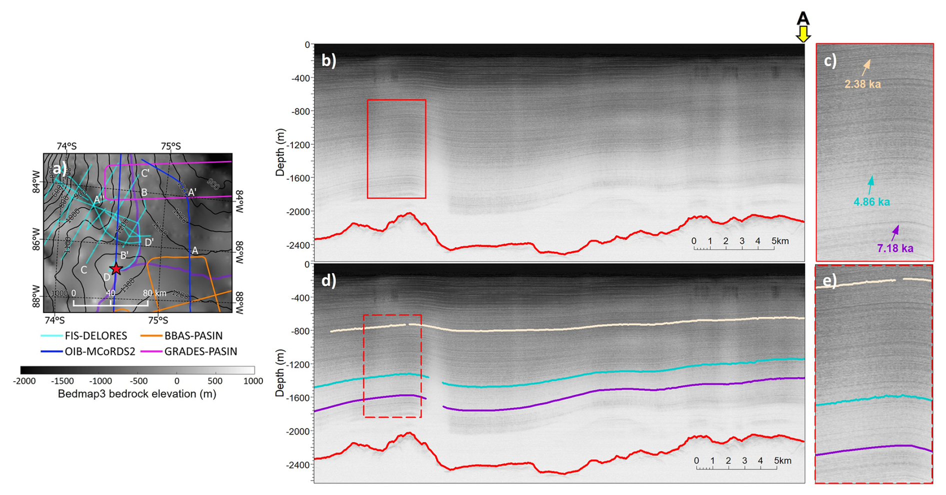
Figure A1 RES profiles showing the location of the onset of IRH tracing in this study, with zoomed views (c, e) highlighting the appearance of the three traced IRHs in more detail. (a) Map of the study area, highlighting key RES datasets used in this study and the ABW site (red star), overlaid on bedrock elevation data from Pritchard et al. (2025), and CryoSat-2 100 m surface-elevation contours from Helm et al. (2014). The ice divides of the Bellingshausen, Amundsen, and Weddell Sea drainage basins are shown in purple (Zwally et al., 2012). (b)–(e) OIB-MCoRDS2 RES profiles at the intersection (A) with the BBAS-PASIN flight-line, illustrating the appearance of IRHs in the OIB-MCoRDS2 data and their manifestation along the flight-line.

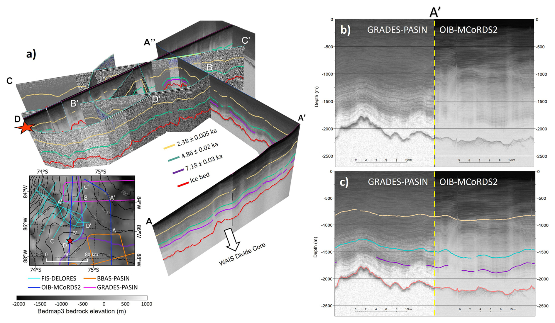
Figure A2 Zoomed-in view of the intersection (A') between the OIB-MCoRDS2 and GRADES-PASIN RES flight-lines. (a) Fig. 2 from the main text. (b)–(c) RES profiles at the crossover between GRADES-PASIN (on the left) and OIB-MCoRDS2 (on the right) without (b) and with IRH traces (c).

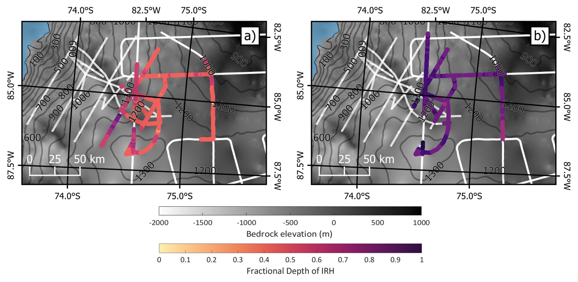
Figure A3 Fractional depths of the 2.38 ka (a) and 4.86 ka (b) IRHs across the Ferrigno Ice Stream catchment. Bedrock elevation data is from Pritchard et al. (2025), and CryoSat-2 100 m surface-elevation contours come from Helm et al. (2014)

Appendix B: Cost function and L-curves

The inverse problem is Sect. 2.4.2 is formulated as finding optimal records of accumulation a(t) that minimise the difference between observations and modelled results. To prevent the model overfitting to the observational data, we conduct L-curve analyses to determine an optimal regularisation parameter following a mathematical approach similar to the one described in Wolovick et al. (2023).

B1 Cost function

In our cost function, we use a single observational misfit and a single regularisation term. Our observational misfit (J_obs) is defined as the mean square error between the observed ages and the modelled age outputs.

$$\begin{array}{}\text{(B1)}& J_{\mathrm{obs}}={\displaystyle \frac{\mathrm{1}}{n}}\sum _{i=\mathrm{1}}^n\left(A\right(d_i,t_i)-A_{\mathrm{obs},i}{)}^{\mathrm{2}}\end{array}$$

where A_obs,i is the observed age, A is the modelled age at depth d and time t, and n represents the number of observations. To penalise high variability between modelled accumulation rate outputs, we employ a regularisation term (J_reg) which is the standard deviation (σ) of the values of a at the tie-points (a_opt) in the piecewise linear function (Sect. 2.4.2).

$$\begin{array}{}\text{(B2)}& J_{\mathrm{reg}}=\mathit{\sigma }\left(a_{\mathrm{opt}}\right)\end{array}$$

The total cost function (J) that is minimised to find optimal records of accumulation, a(t), in Sect. 2.4.2 is:

$$\begin{array}{}\text{(B3)}& J=J_{\mathrm{obs}}+\mathit{\lambda }{J}_{\mathrm{reg}}\end{array}$$

where λ denotes the weight of the Tikhonov regularisation parameter for accumulation. We run the inverse model for a range of λ values and find an optimal range of λ values through L-curve analyses.

B2 L-curves

In Fig. B1a, we plot the values of J_obs and J_reg together in log-log space and a visible “L” can be observed for the range of modelled λ values. An immediate visual inspection of Fig. B1a highlights a range of possible λ values at the corner of the L-curve. For large values of λ, the curve becomes horizontal and the age-depth solution is over-smoothed; this is explicitly shown in Fig. B1c where the gradients of both costs become constant for large λ values. For small λ values the age-depth solution overfits to the input observations, and J_obs is small, so finding an optimal λ value between both of these extremes is crucial to appropriately control the output solution.

To determine an optimal λ value, we compute the first derivatives (Fig. B1c) and second (Fig. B1d) derivatives of both the observational and regularisation components of the cost function. We then sum the cost curvatures for each component of the cost function to derive the total curvature. The location of the maximum total curvature ($\mathit{\lambda }=\sim \mathrm{9000}$) represents the location of the sharpest corner in the L-curve, and thus the optimal λ value. We select this value to use in our model simulations, but a range of λ values where the curvature is greater than half the maximum curvature would likely also be acceptable (Wolovick et al., 2023).

$$\begin{array}{}\text{(B4)}& {\displaystyle }\text{cost gradient}={\displaystyle \frac{\mathrm{d}\left(\ln \right(J\left)\right)}{\mathrm{d}\left(\ln \right(\mathit{\lambda }\left)\right)}}\text{(B5)}& {\displaystyle }\text{cost curvature}={\displaystyle \frac{{\mathrm{d}}^{\mathrm{2}}\left(\ln \right(J\left)\right)}{\mathrm{d}\left(\ln \right(\mathit{\lambda }){)}^{\mathrm{2}}}}\end{array}$$

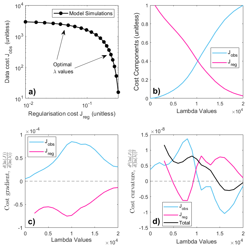
Figure B1 L-curve regularisation to minimise over-fitting to observational data. (a) L-curve from log-log plot of J_obs vs. J_reg. Black circles represent the sampled lambda values, with the red arrows identifying the corner of the L-curve. (b) Plot of both components in the cost function. (c) and (d) represent the cost gradient and cost curvature, respectively, as a function of lambda. Our optimal lambda values (λ=9000) sits at the location of maximum curvature in (d).

Appendix C: Basal melt results

In order to estimate the basal melting at the ABW site, where we cannot constrain the precise GHF, we adopt an approach to estimate basal melt rates from an ice temperature profile estimated using a steady-state temperature model detailed in Jordan et al. (2018). This model calculates the ice temperature at a given depth and time as a function of the vertical velocity similar to the age-depth model described in Sect. 2.4.1. As the GHF at ABW is poorly-constrained (Burton-Johnson et al., 2020), we constrain the model using a range of GHF values (50–140 mW m⁻²) to account for discrepancies between individual GHF data products. We then extract the basal temperature output and calculate melting using Eq. (4) (Leysinger Vieli et al., 2018). The temperature profiles at ABW indicate that the onset of basal melting (when basal temperatures rise above 0 °C) initiates at 67 mW m⁻² (Fig. C1). We calculate melt rates for these conditions to be around 10 mm/yr, rising up to 20 mm yr⁻¹ for the highest GHF (140 mW m⁻²).

In Sect. 4.2, we discuss how prescribing these melt rates influences the modelled age-depth profiles at ABW.

Figure C1 Estimates of basal temperatures derived using a steady-state temperature model (Sect. 2.4.3) and basal melt rates (calculated with Eq. 4) for a range of geothermal heat flux values at ABW. The onset of melting at ABW occurs at 67 mW m⁻².