A spatiotemporal analysis of errors in InSAR SWE measurements caused by non-snow phase changes

Spatially distributed measurements of snow water equivalent (SWE) in mountainous terrain are not currently feasible from existing satellite platforms. The NISAR satellite has the potential to provide high resolution (80 m) SWE measurements on a 12 d orbit cycle over many of Earth’s snowy regions, which would represent a new era of spaceborne snow monitoring. The most promising approach for NISAR SWE measurements uses interferometric synthetic aperture radar (InSAR) techniques to derive the 12 d change in SWE (ΔSWE) from the change in phase between two SAR acquisitions. However, many non-snow factors can also change in this 12 d period which subsequently modulate the SAR phase. These non-snow factors can vary differently in both space and time, and in turn introduce spatially and temporally variable errors into InSAR-derived ΔSWE measurements. Here we explore the effects of six non-snow factors that can affect InSAR phase: electron content of the ionosphere, atmospheric water vapor, atmospheric pressure, soil permittivity, vegetation permittivity, and surface deformation. We show how these factors affect phase-based SWE measurements at 13 SNOTEL stations across the western US, as well as regionally across North America. We consider errors resulting from individual 12 d periods, as well as the cumulative effects of the errors when a timeseries of ΔSWE measurements is integrated to derive peak seasonal SWE.

Ionosphere effects result in the largest cumulative error at all SNOTEL stations in our analysis, with changes in the total electron content resulting in phase changes equivalent to 0.271–0.414 m of SWE, or more than 500 % larger than the median 1 April SWE at some shallow snow stations. When ionosphere effects are removed, the remaining cumulative error ranges from −0.074–0.022 m of SWE, equivalent to 0 %–89 % of 1 April SWE. Relative error results are affected primarily by differences in peak SWE rather than differences in absolute error values. For a randomly selected 12 d period, exceedance probability analysis shows that there is a 50 % chance the ionospheric component introduces an error larger than 0.211 m into the overall ΔSWE measurement, while the remaining five components have a 50 % exceedance probability of 0.031 m. We also find that individual error components can show offsetting effects, where positive and negative biases partially cancel out to lower the total cumulative error. Accurate ΔSWE measurements using NISAR data will not be possible unless ionospheric effects can be appropriately addressed. Removal of other error sources requires careful consideration of the SWE monitoring application: for tracking seasonal SWE accumulation in areas with deeper snowpacks, correcting some errors but not others may actually decrease accuracy by removing offsetting cumulative effects. For individual 12 d periods, wet and dry tropospheric effects (due to changes in water vapor and pressure) should be removed for accurate interpretation of spatial patterns of snow accumulation at basin to range scales, and site-specific factors should be considered to assess the relative influence of vegetation, soils, and surface deformation.

1 Introduction

Snow water equivalent (SWE) measurements derived from interferometric synthetic aperture radar (InSAR) sensors have shown promising accuracy in dry snowpacks. Specifically, at low radar frequencies ($\le \sim \mathrm{10}$ GHz), the dry snowpack is nearly transparent, but causes a signal delay as incident microwave radiation travels to the snow-ground interface and back to the receiver. Changes in the radar time-of-flight from two acquisitions separated in time change the phase of the wave measured at the receiver. These changes in phase can be used to measure changes in SWE (ΔSWE) over the same period by applying differential InSAR techniques (see Marshall and Koh, 2008, for review). Individual ΔSWE measurements can then be integrated through time to track seasonal SWE accumulation. Previous investigations with tower-mounted radars have reported seasonal errors below 9 mm (8 %) SWE (Leinss et al., 2015). A multifrequency tower-mounted radar experiment (Ruiz et al., 2022) demonstrated that lower radar frequencies and shorter temporal baselines (elapsed time between radar acquisitions) result in lower SWE errors, down to 4 mm (3 %) SWE at L-band (∼1.3 GHz) with a 6 h baseline. SWE measurements derived from airborne L-band data show similarly low errors in a variety of snow climates across the western United States (Tarricone et al., 2023; Bonnell et al., 2024a; Hoppinen et al., 2024; Tarricone et al., 2025) and Austrian Alps (Belinska et al., 2024), though challenges still remain where snow is generally difficult to measure, including in dense forests (Bonnell et al., 2024b) and shallow, heterogeneous snowpacks (Palomaki and Sproles, 2023). Additionally, these techniques are applicable primarily during the accumulation season when snow is dry. The presence of significant liquid water in the snowpack strongly attenuates incident radiation and changes the radar velocity, making SWE estimates difficult.

InSAR-derived SWE measurements have also been demonstrated using C-band (∼5 GHz) and L-band satellite data, including from ERS 1/2 (Guneriussen et al., 2001; Rott et al., 2003; Deeb et al., 2011), Sentinel-1 (Oveisgharan et al., 2024), and ALOS-2 (Ruiz et al., 2024). Results from these studies showed that satellite measurements could capture spatial patterns of SWE accumulation, and in some cases showed high correlation to in situ validation data (Oveisgharan et al., 2024). However, none of the satellite platforms used in these studies satisfy spatiotemporal (100 m, 3–5 d) plus accuracy (±10 % for SWE values up to 2.5 m) monitoring requirements for SWE in mountainous regions set in the 2017–2027 National Academies Decadal Survey (National Academies of Sciences, Engineering, and Medicine, 2018). The recently-launched NISAR satellite platform provides L-band (1.257 GHz) InSAR data at 80 m spatial resolution (Brancato et al., 2024) with overlapping ascending and descending passes in its global 12 d orbit cycle, resulting in data acquisition every 3–6 d over many snowy regions. However, NISAR (or any InSAR satellite) phase can be modulated by many non-snow factors which introduce random errors or bias into phase-based SWE measurements. Here we consider six non-snow factors: ionospheric advance, wet and dry tropospheric delay, changes in soil and vegetation permittivity, and land surface deformation. We note that this is a non-exhaustive list of potential error sources. For example, we do not assess errors that arise due to platform-specific factors like temporal decorrelation, which increases uncertainty in the calculated InSAR phase (Zebker and Villasenor, 1992) and subsequently any phase-based measurement. Temporal decorrelation at a given location is affected by local incidence angle, which is determined by the specific imaging geometry of the sensor as well as the radar frequency. Although decorrelation will be an important factor to consider for NISAR SWE measurements, modeling these effects which are also influenced by changing snow conditions is beyond the scope of this work. Instead, we focus on platform-agnostic non-snow factors to quantify the relative magnitude of the errors and illustrate site- and season-specific considerations for improving the accuracy of NISAR SWE measurements. This is an important step to determine if NISAR-derived measurements can meet the 2017–2027 Decadal Survey ±10 % accuracy target.

In this paper we quantify how six non-snow factors influence InSAR phase and introduce error into phase-based SWE measurements and compare the results to measured SWE at SNOTEL stations around the western United States (WUS). We base our analysis on the 12 d change in the non-snow factors to provide a discussion relevant for NISAR and its 12 d orbit cycle. For each non-snow factor, we use observed or modeled data to simulate the phase modulation over a 12 d baseline, then covert that change in phase to the associated (erroneous) change in SWE. In Sect. 2 we provide the governing equations for the error factors and describe our analysis methods. We present results in a cumulative seasonal context in Sect. 3 and in a single 12 d baseline context in Sect. 4. We discuss our findings in Sect. 5 and provide suggestions for minimizing NISAR-derived SWE errors in Sect. 6.

2 Derivation of non-snow errors

2.1 Phase-to-SWE equation

The change in InSAR phase Δϕ_s caused by a change in snow over the same temporal baseline can be calculated as (Guneriussen et al., 2001)

$$\begin{array}{}\text{(1)}& \mathrm{\Delta }{\mathit{\varphi }}_{\mathrm{s}}=-\mathrm{2}\mathit{\kappa }\mathrm{\Delta }{z}_{\mathrm{s}}\left(\cos {\mathit{\theta }}_{\mathrm{i}}-\sqrt{\mathit{\epsilon }-{\sin }^{\mathrm{2}}{\mathit{\theta }}_{\mathrm{i}}}\right)\end{array}$$

where $\mathit{\kappa }=\mathrm{2}\mathit{\pi }/\mathit{\lambda }$ is the wavenumber, Δz_s is the change in snow depth in m, θ_i is the incidence angle in radians, and ε is the bulk snowpack permittivity. The factor of 2 at the beginning of the equation accounts for the two-way travel time between the transmitter and the target. The bulk snowpack permittivity of dry snow can be approximated by snow density, but spatially distributed measurements of either permittivity or density are rarely available and both are difficult to model accurately. Using an empirical approximation to remove the density-dependent term (Leinss et al., 2015) and multiplying snow depth and snow density to obtain SWE, Eq. (1) can be rearranged to solve for directly for ΔSWE as

$$\begin{array}{}\text{(2)}& \mathrm{\Delta }\text{SWE}=\mathrm{\Delta }{\mathit{\varphi }}_{\mathrm{s}}\cdot {\displaystyle \frac{\mathit{\lambda }}{\mathrm{2}\mathit{\pi }\mathit{\alpha }}}{\left(\mathrm{1.59}+{\mathit{\theta }}_{\mathrm{i}}^{\mathrm{5}/\mathrm{2}}\right)}^{-\mathrm{1}}\end{array}$$

More details of this derivation can be found in Leinss et al. (2015) and Palomaki and Sproles (2023). Despite additional error introduced by the empirical approximation (Leinss et al., 2015), Eq. (2) is better suited than Eq. (1) for use with satellite-derived SWE measurements because it does not require snow density as an input. We use Eq. (2) to derive the non-snow error equations in the next section. For our analysis in this paper, we fix α=1 (for which retrieval error is below 7 % for θ<50°; Leinss et al., 2015), θ_i=40° (0.698 rad; approximately the average incidence angle for NISAR scenes) and λ=0.2385 m (NISAR L-band wavelength) in Eq. (2).

2.2 Non-snow error equations

Surface and atmospheric conditions other than SWE that change over a 12 d period can modulate the measured InSAR phase and introduce errors into the SWE retrieval. Here we consider six non-snow factors (Table 1): ionospheric effects (changes in total electron content), wet tropospheric effects (changes in atmospheric water vapor), dry tropospheric effects (changes in atmospheric pressure), soil permittivity (primarily changes in soil moisture), vegetation permittivity (primarily changes in air temperature), and surface deformation (changes in surface elevation). For this analysis we quantify errors in InSAR-derived SWE by calculating Δϕ associated with a given non-snow factor, then use Eq. (2) to calculate the error in ΔSWE resulting from the non-snow related Δϕ. For clarity in several of the following derivations, we make the substitution $\mathrm{2}\mathit{\kappa }=\mathrm{4}\mathit{\pi }/\mathit{\lambda }$. Throughout the analysis, negative errors mean that the measured ΔSWE is underestimated compared to the true change, and positive errors indicate overestimated SWE change.

Table 1 Data sources and characteristics for non-snow error factors.

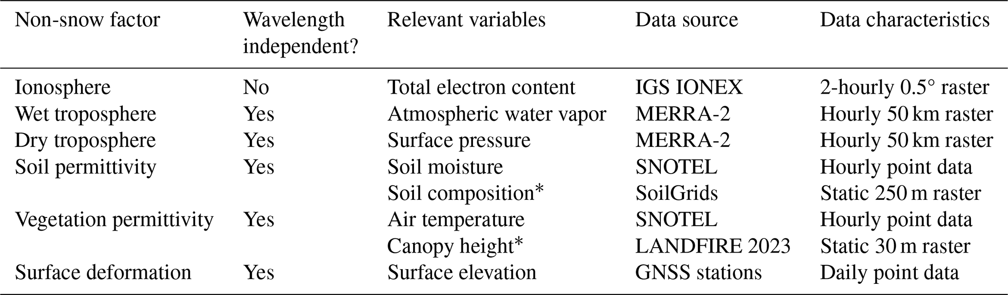
^∗ assumed constant over 12 d.

2.2.1 Ionospheric error

Changes in the vertically integrated total electron content ΔTEC in the ionosphere affect the InSAR phase. The varying electron density of the ionosphere is affected by solar UV radiation, Earth's magnetic field, and atmospheric gas concentrations; interactions between these factors cause electron density concentrations to vary over multiple spatial (sub-kilometer to tens of kilometers) and temporal (diurnal, seasonal, and interannual) scales (Lean et al., 2016). The resulting impacts on InSAR phase are frequency-dependent and can introduce larger errors at lower frequencies, like NISAR's L-band measurements (Meyer and Agram, 2017). The phase change Δϕ_ion due to ΔTEC in units of TECU (10¹⁶ electrons per m²) is

$$\begin{array}{}\text{(3)}& \mathrm{\Delta }{\mathit{\varphi }}_{\text{ion}}=-{\displaystyle \frac{\mathrm{4}\mathit{\pi }K\mathit{\lambda }}{c^{\mathrm{2}}}}\mathrm{\Delta }\text{TEC}\end{array}$$

where K is a constant (40.28 m³ s⁻²) and c is the speed of light (Rosen et al., 2010). Inserting Δϕ_ion from Eq. (3) into Eq. (2) we obtain

$$\begin{array}{}\text{(4)}& \mathrm{\Delta }{\text{SWE}}_{\text{ion}}\left(\mathrm{\Delta }\text{TEC}\right)=-{\displaystyle \frac{\mathrm{2}K{\mathit{\lambda }}^{\mathrm{2}}}{c^{\mathrm{2}}\mathit{\alpha }(\mathrm{1.59}+{\mathit{\theta }}_{\mathrm{i}}^{\mathrm{5}/\mathrm{2}})}}\mathrm{\Delta }\text{TEC}\end{array}$$

At a fixed θ_i=40°, this corresponds to 0.258 m of SWE error per unit increase of TEC for NISAR-derived measurements. The negative indicates this non-snow factor causes a phase advance while most other factors cause phase delays. We use Eq. (4) to calculate ionospheric error in our analysis using TEC data from IGS IONEX (Schaer et al., 1998).

2.2.2 Tropospheric errors

Temporal variation in water vapor, temperature, and air pressure in the troposphere affect the InSAR phase. These tropospheric effects are typically separated into two components (Jolivet et al., 2014). The first is the wet delay Δϕ_wet, a function of changes in water vapor pressure e and air temperature T given by

$$\begin{array}{}\text{(5)}& \mathrm{\Delta }{\mathit{\varphi }}_{\text{wet}}={\displaystyle \frac{\mathrm{4}\mathit{\pi }}{\mathit{\lambda }}}{\displaystyle \frac{{\mathrm{10}}^{-\mathrm{6}}}{\cos \left({\mathit{\theta }}_{\mathrm{i}}\right)}}\underset{z_{\text{surf}}}{\overset{z_{\text{ref}}}{\int }}\left(k_{\mathrm{2}}-{\displaystyle \frac{R_{\mathrm{d}}}{R_{\mathrm{v}}}}{k}_{\mathrm{1}}\right){\displaystyle \frac{\mathrm{\Delta }e}{\mathrm{\Delta }T}}+k_{\mathrm{3}}{\displaystyle \frac{\mathrm{\Delta }e}{\mathrm{\Delta }{T}^{\mathrm{2}}}}\mathrm{d}z\end{array}$$

where k₁, k₂, and k₃ are constants (0.776 K Pa⁻¹, 0.716 K Pa⁻¹, and 3.75×10³ K² Pa⁻¹, respectively), R_v is the specific gas constant for water vapor (461.52 $\mathrm{J}{\mathrm{kg}}^{-\mathrm{1}}{\mathrm{K}}^{-\mathrm{1}}$), z_surf is the surface height and z_ref is a high altitude reference height representing the top of the atmospheric column. By integrating the column water vapor into the meters of precipitable water (PW) and using an average atmospheric temperature, we can approximate the phase change Δϕ_PW due to ΔPW as

$$\begin{array}{}\text{(6)}& \mathrm{\Delta }{\mathit{\varphi }}_{\text{wet}}={\displaystyle \frac{\mathrm{4}\mathit{\pi }}{\mathit{\lambda }}}{\displaystyle \frac{\mathrm{6.5}}{\cos \left({\mathit{\theta }}_{\mathrm{i}}\right)}}\mathrm{\Delta }\text{PW}\end{array}$$

The relative error in this estimate is approximately equal to the error in the average atmospheric temperature estimate, which in reality can vary by up to 20 % (Bevis et al., 1994). Inserting Δϕ_wet from Eq. (6) into Eq. (2) we obtain

$$\begin{array}{}\text{(7)}& \mathrm{\Delta }{\text{SWE}}_{\text{wet}}\left(\mathrm{\Delta }\text{PW}\right)={\displaystyle \frac{\mathrm{2}}{\mathit{\alpha }(\mathrm{1.59}+{\mathit{\theta }}_{\mathrm{i}}^{\mathrm{5}/\mathrm{2}})}}{\displaystyle \frac{\mathrm{6.5}}{\cos {\mathit{\theta }}_{\mathrm{i}}}}\mathrm{\Delta }\text{PW}\end{array}$$

The wet delay is the main contributor to tropospheric phase delay (Jolivet et al., 2014). At a fixed θ_i=40°, this corresponds to 8.516 m of SWE error per meter of ΔPW. We use Eq. (7) to calculate the wet tropospheric error in our analysis using precipitable water data from MERRA-2 (Global Modeling And Assimilation Office and Pawson, 2015).

The second and typically smaller tropospheric error component is the hydrostatic delay (also referred to as the dry or stratified delay) due to changes in air pressure P (Jolivet et al., 2014). The dry delay Δϕ_dry is given by

$$\begin{array}{}\text{(8)}& \mathrm{\Delta }{\mathit{\varphi }}_{\text{dry}}={\displaystyle \frac{\mathrm{4}\mathit{\pi }}{\mathit{\lambda }}}{\displaystyle \frac{{\mathrm{10}}^{-\mathrm{6}}}{\cos \left({\mathit{\theta }}_{\mathrm{i}}\right)}}{\displaystyle \frac{k_{\mathrm{1}}{R}_{\mathrm{d}}}{g_m}}\mathrm{\Delta }P\left(z\right)\end{array}$$

where R_d is the specific gas constant for dry air (287.05 $\mathrm{J}{\mathrm{kg}}^{-\mathrm{1}}{\mathrm{K}}^{-\mathrm{1}}$), g_m is the local gravitational acceleration (assumed static at 9.81 m s⁻²), and ΔP(z) is the change in relative air pressure in Pa. Inserting Δϕ_dry from Eq. (8) into Eq. (2) we obtain

$$\begin{array}{}\text{(9)}& \begin{array}{rl}\mathrm{\Delta }{\text{SWE}}_{\text{dry}}\left(\mathrm{\Delta }P\right(z\left)\right)& ={\displaystyle \frac{\mathrm{2}}{\mathit{\alpha }(\mathrm{1.59}+{\mathit{\theta }}_{\mathrm{i}}^{\mathrm{5}/\mathrm{2}})}}\\ & \cdot {\displaystyle \frac{{\mathrm{10}}^{-\mathrm{6}}}{\cos \left({\mathit{\theta }}_{\mathrm{i}}\right)}}{\displaystyle \frac{k_{\mathrm{1}}{R}_{\mathrm{d}}}{g_m}}\mathrm{\Delta }P\left(z\right)\end{array}\end{array}$$

At a fixed θ_i=40°, this corresponds to 0.0297 m of SWE error per kPa change in air pressure. We use Eq. (9) to calculate the wet tropospheric error in our analysis using surface pressure data from MERRA-2 (Global Modeling And Assimilation Office and Pawson, 2015). It is important to note that both dry and wet tropospheric effects vary with elevation, since radar waves must travel through more of the atmosphere to reach lower altitudes. This elevation dependence can produce patterns tropospheric effects that resemble those associated with snow accumulation or ablation.

2.2.3 Soil permittivity errors

At L-band frequencies some radar energy will typically penetrate into the soil medium at the snow-ground interface. The soil permittivity, which influences the speed of radar waves in soil, is controlled primarily by soil composition and moisture content. Assuming the soil is isotropic, uniform, and linear, De Zan et al. (2014) showed that the phase change Δϕ_soil due to changes in soil permittivity can be calculated using

$$\begin{array}{}\text{(10)}& \mathrm{\Delta }{\mathit{\varphi }}_{\text{soil}}={\displaystyle \frac{\mathrm{1}}{\mathrm{2}j{k}_{z\mathrm{1}}^{\prime }-\mathrm{2}j{k^{\prime }}_{z\mathrm{2}}^{*}}}\end{array}$$

where $k_{z\mathrm{1}}^{\prime }$ and $k_{z\mathrm{2}}^{\prime }$ are the vertical soil wavenumbers at the first and second radar acquisitions, respectively, and the * operator denotes the complex conjugate. The vertical soil wavenumber $k_z^{\prime }$ can be expressed as

$$\begin{array}{}\text{(11)}& k_z^{\prime }=\sqrt{{\mathit{\omega }}^{\mathrm{2}}{\mathit{ϵ}}^{\prime }\mathit{\mu }-k_x^{\mathrm{2}}}\end{array}$$

where ω=κc is the angular frequency of the radar wave, ϵ^′ is the real component of the soil dielectric permittivity, μ is the soil magnetic permeability, and k_x=κsin θ_i is the horizontal wavenumber of free air. For most soils, magnetic permeability is approximately equal to 1 at low radar frequencies (Patitz et al., 1995; Youn et al., 2010). The real part of the dielectric permittivity is a function of frequency, water content, and soil type (e.g., clay, silt, and sand fractions). Using polynomial approximations for the real component of soil dielectric permittivity (Hallikainen et al., 1985), we estimate SWE error using Eqs. (10) and (11) for a variety of soil types based on changes in soil moisture (Fig. 1). The largest soil-related SWE errors occur when moisture changes in relatively dry soils, with errors leveling off with moisture changes in wetter soils. Soils of various compositions show similar trends, with increasing clay content associated with smaller dielectric changes and associated SWE errors. For our analysis we use soil composition data from SoilGrids (Poggio et al., 2021) and soil moisture data from SNOTEL sites.

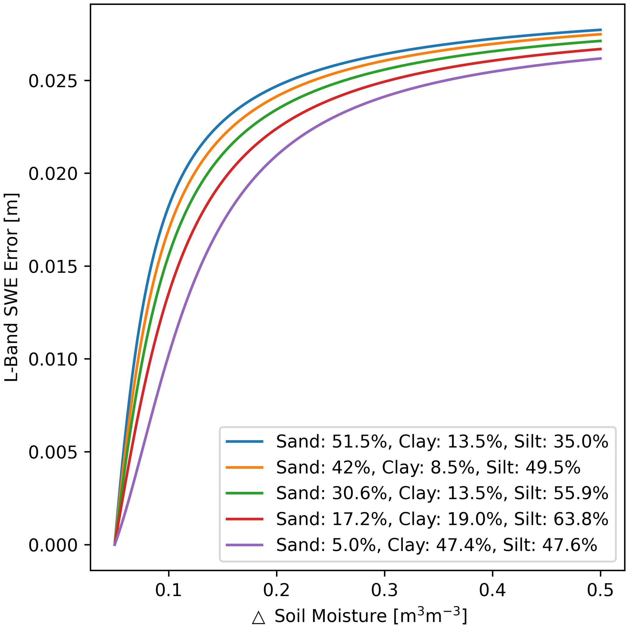
Figure 1 Example L-band SWE error curves for five soil types based on soil moisture content to avoid erratic polynomial effects, soil moisture content starts at 0.05 m³ m⁻³.

2.2.4 Vegetation permittivity errors

Subfreezing air temperatures can cause liquid water within vegetation to freeze. The transition from liquid water to ice within wood affects the dielectric permittivity of trees (Schwank et al., 2021). To calculate the phase change Δϕ_veg due to changes in vegetation permittivity we use the mixing model between wood, water, air, and ice given by Schwank et al. (2021):

$$\begin{array}{}\text{(12)}& \mathrm{\Delta }{\mathit{\varphi }}_{\text{veg}}={\displaystyle \frac{\mathrm{4}\mathit{\pi }}{\mathit{\lambda }}}H\left(\sqrt{{\mathit{ϵ}}_{\text{c,2}}-{\sin }^{\mathrm{2}}\left({\mathit{\theta }}_{\mathrm{i}}\right)}-\sqrt{{\mathit{ϵ}}_{\text{c,1}}-{\sin }^{\mathrm{2}}\left({\mathit{\theta }}_{\mathrm{i}}\right)}\right)\end{array}$$

where H is the canopy height and the canopy permittivity ϵ_c at time 1 and 2 is defined by

$$\begin{array}{}\text{(13)}& {\mathit{ϵ}}_{\mathrm{c}}={\mathit{ϵ}}_{\text{air}}+{\displaystyle \frac{({\mathit{ϵ}}_{\text{wood}}-{\mathit{ϵ}}_{\text{air}})({\mathit{ϵ}}_{\text{wood}}+\mathrm{5}{\mathit{ϵ}}_{\text{air}})v_{\text{SCC}}}{\mathrm{3}({\mathit{ϵ}}_{\text{wood}}+{\mathit{ϵ}}_{\text{air}})-\mathrm{2}({\mathit{ϵ}}_{\text{wood}}-{\mathit{ϵ}}_{\text{air}})v_{\text{SCC}}}}\end{array}$$

where v_SCC is the volume fraction of space occupied by small canopy constituents (branches, stems, trunks), ϵ_air is the permittivity of free air, and ϵ_wood is the permittivity of wood. Wood permittivity is calculated from the porosity and density of the wood combined with wood cell, water, and ice permittivities and ratios as

$$\begin{array}{}\text{(14)}& \begin{array}{rl}{\mathit{ϵ}}_{\text{wood}}& =v_{{\mathrm{H}}_{\mathrm{2}}\mathrm{O}}{\mathit{ϵ}}_{{\mathrm{H}}_{\mathrm{2}}\mathrm{O}}+(\mathrm{1}-\text{por}){\mathit{ϵ}}_{\text{wood-cell}}\\ & +(\text{por}-v_{{\mathrm{H}}_{\mathrm{2}}\mathrm{O}}){\mathit{ϵ}}_{\text{air}}\end{array}\end{array}$$

We assume that the only temporally variable parameter in winter is permittivity of the water within the wood, which is controlled by the the water-to-ice ratio within the wood cell (v_water):

$$\begin{array}{}\text{(15)}& {\mathit{ϵ}}_{{\mathrm{H}}_{\mathrm{2}}\mathrm{O}}=v_{\text{water}}{\mathit{ϵ}}_{\text{water}}+(\mathrm{1}-v_{\text{water}}){\mathit{ϵ}}_{\text{ice}}\end{array}$$

While direct measurements of ice-water ratio within wood are challenging, we use the approximation using air temperature T given in Schwank et al. (2021):

$$\begin{array}{}\text{(16)}& v_{\text{water}}\left(T\right)=\left\{\begin{array}{ll}\mathrm{1},& \text{if }T>\mathrm{0}\mathrm{°}\mathrm{C}\\ \exp \left(\frac{T}{T_{\text{melt}}}\right),& \text{if }T\le \mathrm{0}\mathrm{°}\mathrm{C}\end{array}\right.\end{array}$$

We use Eqs. (12) through (16) to calculate the vegetation permittivity error in our analysis using air temperature data from SNOTEL and canopy height data from LANDFIRE (Dewitz, 2026). For all constant parameters in Eqs. (12) through (16) we use values in Table 1 of Schwank et al. (2021).

2.2.5 Surface deformation

Changes in surface elevation change the line-of-sight distance between the ground and the sensor. Surface elevation can shift due to many factors, including earthquakes, subsidence, solid earth and ocean tides, and permafrost thaw. The phase change Δϕ_R due to surface elevation change ΔR is given by

$$\begin{array}{}\text{(17)}& \mathrm{\Delta }{\mathit{\varphi }}_R={\displaystyle \frac{\mathrm{4}\mathit{\pi }}{\mathit{\lambda }}}\mathrm{\Delta }R\end{array}$$

Inserting Δϕ_R from Eq. (17) into Eq. (2) we obtain

$$\begin{array}{}\text{(18)}& \mathrm{\Delta }{\text{SWE}}_{\text{def}}\left(\mathrm{\Delta }R\right)={\displaystyle \frac{\mathrm{2}}{\mathit{\alpha }(\mathrm{1.59}+{\mathit{\theta }}_{\mathrm{i}}^{\mathrm{5}/\mathrm{2}})}}\mathrm{\Delta }R\end{array}$$

At a fixed θ_i=40°, this corresponds to 1.001 m of SWE error per meter of surface deformation. We use Eq. (18) to calculate the surface deformation error in our analysis using surface elevation data from GNSS stations.

2.3 Error analysis methods

We consider two potential applications of InSAR-based SWE measurements. The first is estimating 1 April SWE by integrating a regular 12 d timeseries of ΔSWE measurements (i.e., from nearest-neighbor interferograms) over the accumulation season. In this application the non-snow errors from any one interferogram are less important than the cumulative error at the time of peak SWE. Because the total error from non-snow factors can be either positive or negative for any single InSAR pair, integrated SWE measurements could have smaller cumulative error if positive and negative errors cancel out over time. The second application is quantifying changes in the spatial distribution of snow across a landscape within a single 12 d period. In this case we are interested in a comparison of the non-snow errors relative to a single ΔSWE value, not the total accumulated SWE.

To illustrate how non-snow errors vary across snow climates, we applied our analysis at locations across the WUS representing 13 major mountain ecoregions denoted by Trujillo and Molotch (2014). We chose a 10 year period between water years 2016–2025 (1 October 2015 through 30 September 2025), which includes high (2023), average (2022), and low (2016) snow seasons, to examine the temporal variability of the errors. All other datasets we use to calculate the non-snow errors (Table 1) are also available for water years 2016–2025. Within each ecoregion, stations were selected based on data availability (98 % complete data records for SWE, air temperature, and 2 inch soil moisture for each of the 10 seasons). When more than one station in an ecoregion met the data availability criteria, we selected so that the final 13 stations span a range of snow classes (Sturm and Liston, 2021), vegetation types and heights, and other environmental characteristics (Table 2).

Table 2 Site Characteristics.

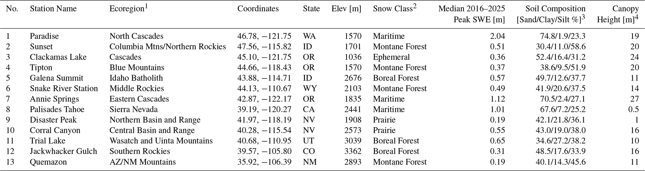
¹ after Trujillo and Molotch (2014); ² after Sturm and Liston (2021); ³ from SoilGrids dataset; ⁴ from LANDFIRE 2024 dataset.

At each station we apply all error calculations using a 12 d moving window with a step size of one day to simulate all possible NISAR acquisitions. An example for soil permittivity error for water year 2021 at the Paradise station is shown in Fig. 2. First, we use the daily soil moisture data (Fig. 2a) to calculate a daily timeseries of soil permittivity error (Fig. 2b) by applying Eq. (10) on a 12 d moving window. In this example we used data from September 2020 in order to get a valid error value on 1 October. Cumulative error calculations are then applied to the daily timeseries over all possible 12 d baselines, again with a moving window of one day (e.g., 1, 13, 25, … October; 2, 14, 26, … October) (Fig. 2c). We combine all possible 12 d cycles into a single daily timeseries, then compute a rolling 12 d mean of the cumulative error to remove cyclic artifacts (Fig. 2d). In our analysis and figures below we use the rolling 12 d cumulative error (orange line in Fig. 2d) in the context of seasonal SWE errors (Sect. 3), and the daily error timeseries (Fig. 2b) in the context of individual 12 d baseline errors (Sect. 4).

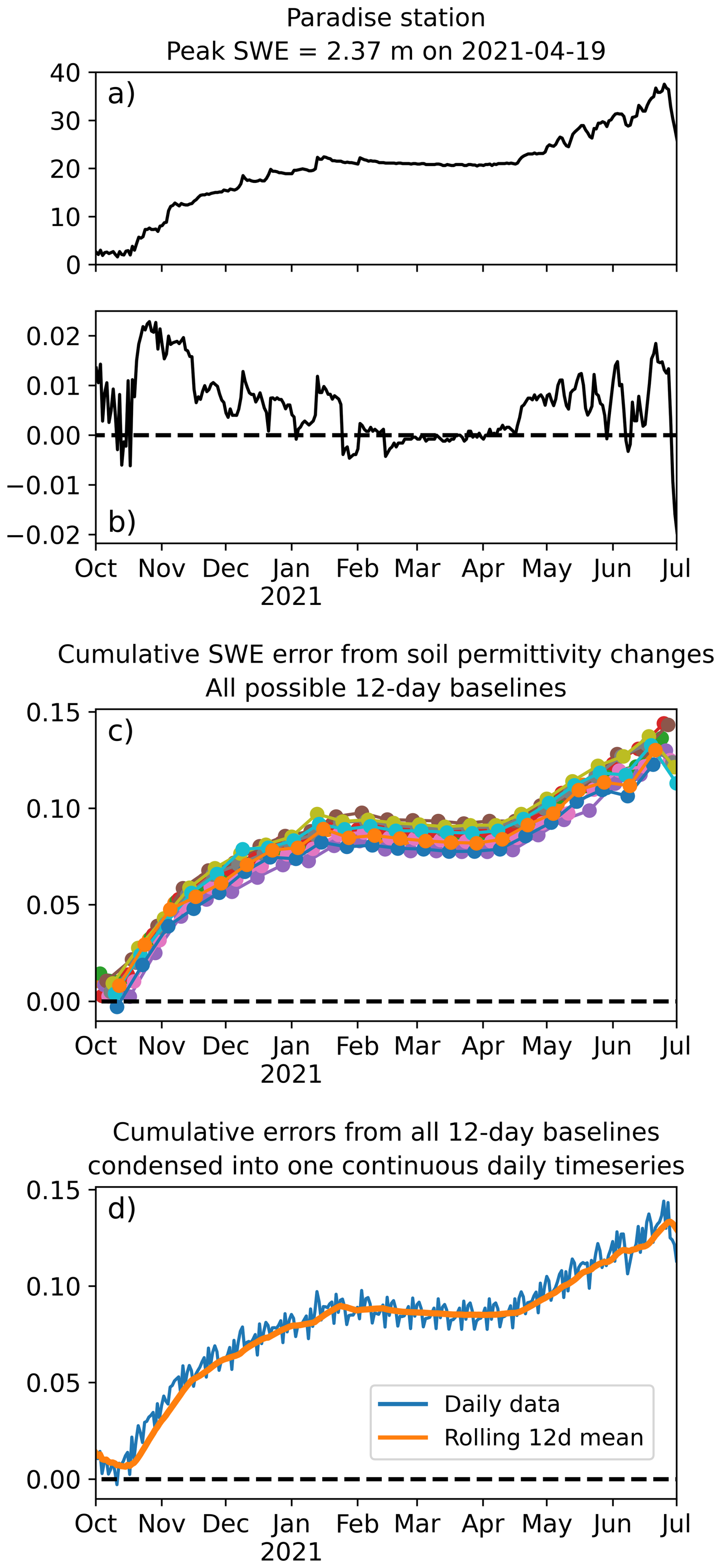
Figure 2 Workflow example using soil moisture changes at the Paradise SNOTEL. Changes in soil moisture (a) result in changes in soil permittivity, a non-snow error component for InSAR SWE measurements. First, we calculate the resulting SWE error for each 12 d pair in the timeseries (b). We then apply cumulative error calculations to the daily timeseries over all possible 12 d baselines (c). Finally, all possible 12 d cumulative error baselines are combined and we apply a rolling 12 d mean (d).

As noted in Table 1, the data sources we use to calculate the non-snow errors have different characteristics (e.g., point data vs. rasters of various resolutions). When raster datasets are used as input to error calculations, we use the value of the pixel that contains the SNOTEL station used for comparison. For surface deformation calculations, we make the assumption that the 12 d surface deformation at a given SNOTEL site is equivalent to that of the nearest GNSS station, even though the SNOTEL and GNSS points are not co-located. We do not attempt to spatially interpolate or otherwise adjust the GNSS data to account for the separation distance.

3 Tracking seasonal SWE: cumulative error analysis

Examples of measured SWE and simulated non-snow InSAR errors are shown for three SNOTEL stations (Fig. 3). Different water years were selected at the different stations only to illustrate how results change in snowpacks of varying depths. Panels in the top row show measured SWE at a given SNOTEL station with the cumulative non-snow errors added to the measured SWE curves. We include separate curves with (grey) and without (orange) the ionosphere error because it can be an order of magnitude larger than the other errors. These are idealized scenarios where the SWE changes recorded by the SNOTEL station can be retrieved exactly once the six non-snow errors are removed. The additional error of up to 7 % introduced by using the density-independent approximation (Eq. 2) is not reflected. Panels in the bottom row show cumulative individual error components over time. We removed the ionosphere error from these panels to better show the detail of the other error components (dry and wet troposphere, vegetation and soil permittivity, and surface deformation).

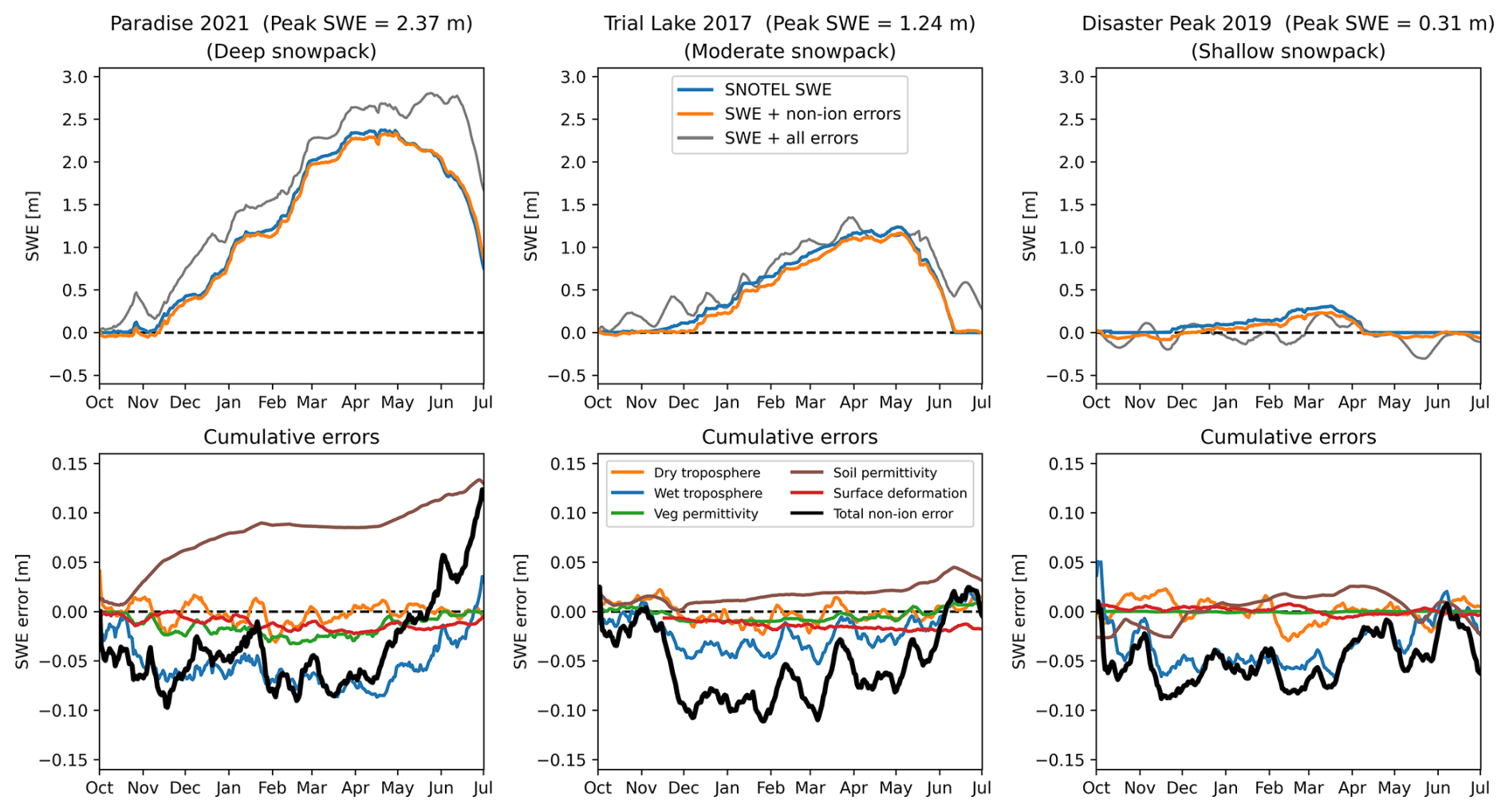
Figure 3 Top row: SNOTEL SWE curves (blue), simulated InSAR-derived SWE curves including non-ionospheric error sources (orange), and simulated InSAR-derived SWE curves including all error sources (gray). Bottom row: Cumulative error for individual error components and total non-ionospheric error. In both rows, the legends shown in the second column apply to all panels in the row.

Individual error components (Fig. 3, bottom row) have partially offsetting effects at the three stations. For example, at all stations the cumulative soil permittivity error introduces a consistent positive bias by the middle of the accumulation season while the wet troposphere error introduces a negative bias during the same period. The dry troposphere error is the closest to unbiased random noise, with the cumulative error fluctuating around 0 cm during the accumulation season at all stations. These three examples all show negative total cumulative errors (thick black lines) for non-ionospheric components over most of the accumulation season.

Figure 3 shows only one season at three stations. We repeat this analysis for multiple years (2016–2025) at multiple stations to investigate the interannual variability of total non-ionospheric cumulative errors. A summary of the total error integrated between 1 October and 1 April gives more evidence of a trend toward negative total cumulative errors on 1 April (Fig. 4). If this error is not removed from the InSAR phase, the overall effect at these stations is that InSAR-derived SWE measurements will tend to underestimate 1 April SWE. However, the interannual variability of the total cumulative error (i.e., the width of the boxplot) changes between stations and most stations also show positive errors (overestimated SWE) in at least one year. This indicates that it may be difficult to predict the general behavior of the total error at any site based on errors measured in previous seasons. For example, at Sunset the largest positive error (0.096 m) occurred in 2016 and the largest negative error (−0.191 m) occurred in 2025, but peak SWE measurements in the two years were very similar (0.452 m in 2016 and 0.444 m in 2025). Wide interannual variability at a site is likely driven by the complex interactions between the error factors and their physical drivers at seasonal scales. For example, a series of several early season snow accumulation/melt events would likely result in fluctuating tropospheric effects (i.e., changes in air pressure and precipitable water associated with frontal passage) but the secondary soil permittivity effects from melting snow are partially controlled by antecedent soil moisture conditions, which we do not assess in our analysis.

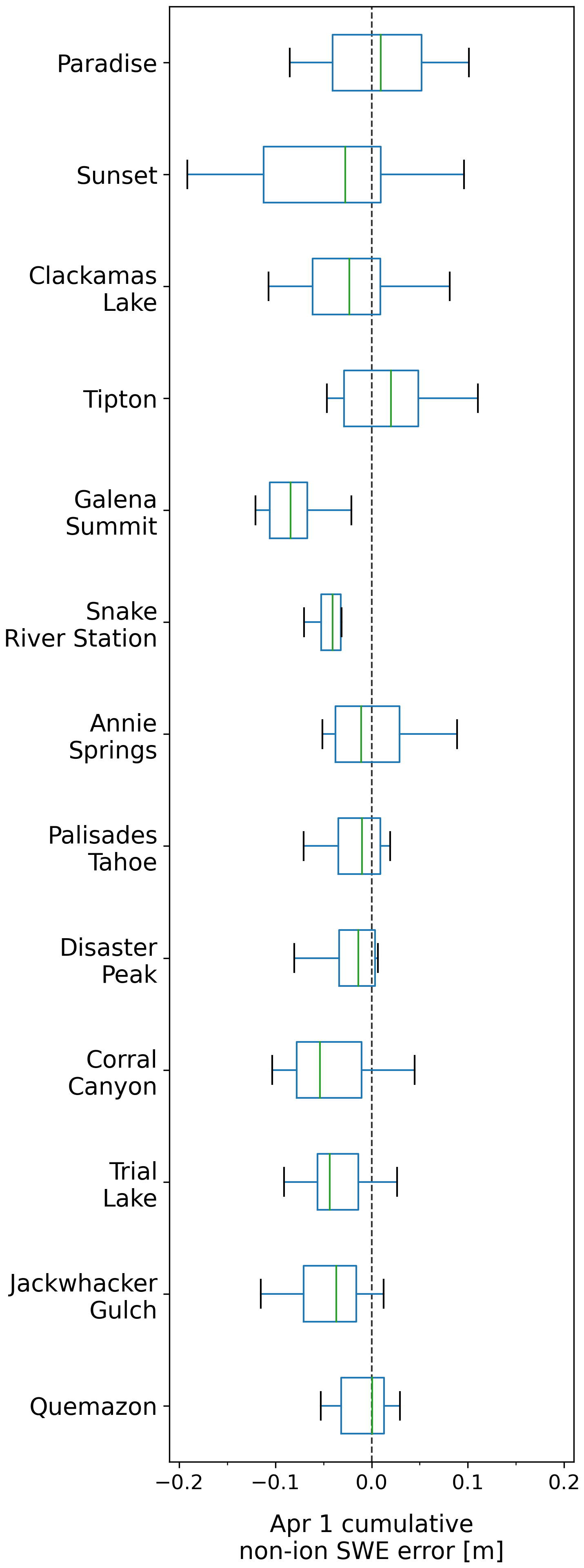
Figure 4 Boxplots summarizing total cumulative non-ionospheric errors on 1 April for 10 seasons (2016–2025) at 13 SNOTEL stations (Table 2).

Results in Fig. 4 also show median cumulative errors on 1 April at all sites are between ±0.1 m of SWE. Whether this represents a significant error at any given station depends on the average 1 April SWE. The inset bar charts in Fig. 5 show how the average cumulative errors compare to the average 1 April SWE at each station. Cumulative errors are calculated each year between 1 October and 1 April for water years 2016–2025, averaged over the 10 water years, and divided by the average 1 April SWE. The different colored bars represent different error types, with the total non-ionospheric error shown in black. All inset axes are clipped to ±10 % of average 1 April SWE on the y axis. Cumulative error components that extend beyond this range are indicated with an arrowhead at the end of the bar. Again we have removed the ionosphere error from this figure to better visualize the other error components. All cumulative errors, including the ionosphere component, are also listed in Table 3 as absolute values and percentages of 1 April SWE at each station.

Figure 5 Average cumulative non-snow errors relative to average 1 April SWE at 13 SNOTEL stations, with consistent y axis scales shown in the bottom inset. Averages are calculated over a 10 year period from water years 2016–2025. In the inset bar charts, the black bars represent the total non-ionospheric error with other colors showing individual error components. The vertical extent of all inset charts are clipped to ±10 % of 1 April SWE for the given station with horizontal dashed lines indicating ±5 %. Error components that extend beyond this range are indicated with an arrowhead at the end of the bar. Station points are colored by snow class (Sturm and Liston, 2021) and the background shows average 1 April SWE calculated using an 800 m reanalysis product (Broxton et al., 2019).

Table 3 Average cumulative errors calculated from 1 October to 1 April over water years 2016–2025. Errors are given as absolute values in meters as well as percentages relative to average 1 April SWE at each station.

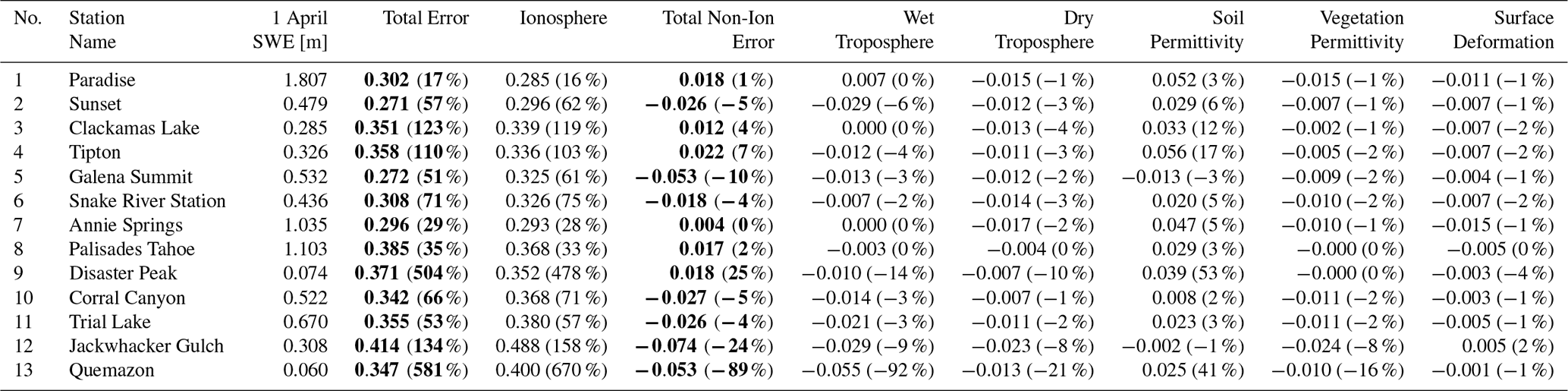
The average 2016–2025 total cumulative error ranges across stations between 0.271–0.414 m, and at all stations is larger than 10 % of 1 April SWE (Table 3). The stations with the deepest average 1 April snowpack (Paradise, Palisades Tahoe, and Annie Springs) have the smallest relative total errors (17 %, 29 %, and 35 %, respectively). Two stations with shallow snow (Disaster Peak and Quemazon) have total errors larger than 500 % of average 1 April SWE, which is less than 0.1 m at both stations. At these low-elevation locations, 1 April may not be an appropriate date to use as a proxy for peak SWE. For example, at Disaster Peak in water year 2019 much of the accumulated SWE had already melted by 1 April (Fig. 3). Shifting the cumulative error calculation to an earlier date would slightly improve these results at Disaster Peak and Quemazon, but we expect that these shallow snowpack stations would still have the largest errors because we report our results relative to average SWE. We do not note any obvious trends in performance solely based on snow class.

The cumulative ionosphere error is the largest error component. At all stations it introduces a large positive bias that represents the vast majority of the total cumulative error. Again we note that the ionosphere error is the only non-snow factor considered here that is a function of the radar frequency, with larger errors at lower frequencies (Rosen et al., 2010). The results in Table 3 show the importance of correcting for ionospheric effects when using L-band data to derive InSAR SWE measurements. While the NISAR platform has a dedicated subband offset from the main instrument frequency to allow for measurement of the dispersive ionospheric effects, other L-band platforms (e.g. ALOS-2) may require advanced data processing techniques like a split-spectrum approach (Wegmüller et al., 2018) to remove ionospheric effects. Additionally, it is possible for NISAR to operate in a quasi-quad-pol configuration utilizing subband data that prevents ionospheric corrections. NISAR data collected in this configuration will require advanced processing techniques before the phase information can be used for SWE retrievals.

At most stations, removing the ionosphere error brings the remaining cumulative error to within ±10 % of 1 April SWE, meeting accuracy targets established in the 2017–2027 Decadal Survey. Soil permittivity errors tend to introduce positive biases into the cumulative error. As illustrated at Paradise during water year 2021 (Fig. 3), this error can increase quickly at the beginning of the water year as early season snow accumulation and melt events influence the soil moisture. The cumulative soil permittivity error remains relatively constant in the middle of the accumulation season with colder temperatures and deeper snowpacks. The remaining components (wet and dry troposphere, vegetation permittivity, and surface deformation) tend to introduce smaller negative biases as they are influenced by meteorological factors (atmospheric water vapor, surface pressure, and air temperature) that fluctuate at daily to weekly timescales.

Total non-ionospheric error is still outside ±10 % at Disaster Peak, Jackwhacker Gulch, and Quemazon (stations 9, 12, and 13, respectively). As discussed previously, these results at Disaster Peak and Quemazon are influenced by very small values for average 1 April SWE. A comparison of results at Jackwhacker Gulch, Tipton (station 4), and Clackamas Lake (station 3) makes for a more interesting discussion. All stations have relatively shallow snowpacks on 1 April (0.308, 0.326, and 0.285 m, respectively) but Jackwhacker Gulch does not meet the Decadal Survey accuracy target with −24 % total non-ionospheric error while the Tipton and Clackamas Lake results do (7 % and 4 %, respectively). The wet troposphere, dry troposphere, and vegetation permittivity errors at the three sites all negatively bias the cumulative error, but the magnitude of the bias for all three components is larger at Jackwhacker Gulch than both Tipton and Clackamas Lake. The difference in magnitudes may be due to differences in station elevations: temporal fluctuations in atmospheric water vapor, surface pressure, and air temperature have different patterns at Jackwhacker Gulch (3362 m in a continental snow climate) compared to Tipton and Clackamas Lake (1570 and 1036 m, respectively, in maritime snow climates). Additionally, at Tipton and Clackamas Lake, positive biases from soil permittivity errors partially offset the other negative biases. Soil permittivity error is much smaller (and negative) at Jackwhacker Gulch, likely a result of its high-elevation setting with consistently cold temperatures throughout the accumulation season, and does not offset the effects from other error components. This example illustrates two important points: (1) the feasibility of InSAR SWE measurements at a given site cannot be determined solely by average snowpack depth but is also controlled by snow climate and other environmental factors, and (2) for non-ionospheric error sources, correcting some errors but not others may actually decrease accuracy by removing effects of offsetting positive and negative biases.

4 Tracking individual SWE events: non-cumulative error analysis

Although some non-snow errors diminish when integrated over the accumulation season, errors within a single 12 d nearest-neighbor interferogram are important considerations for other applications. For example, if a single interferogram is used to examine the spatial variability of snow accumulation from a single event (relevant for avalanche forecasting, for example), non-snow errors can potentially lead to incorrect conclusions about spatial patterns of snow across a landscape. In this context we are interested in absolute values of the non-snow errors as well as their magnitude relative to a single ΔSWE value, not the total accumulated SWE on a particular date. Figure 6 shows the seasonal variability of the six non-snow error components using data from 10 water years (2016–2025) for the same three SNOTEL stations as in Fig. 3. The thick blue line indicates the median error for a given day during the 10 year period, with shading between the interquartile range (25th–75th percentiles). For the ionosphere error (bottom row) we show the 12 d error calculated for at both 06:00 LT (representative of NISAR sampling during ascending orbits) and 18:00 LT (NISAR descending orbits).

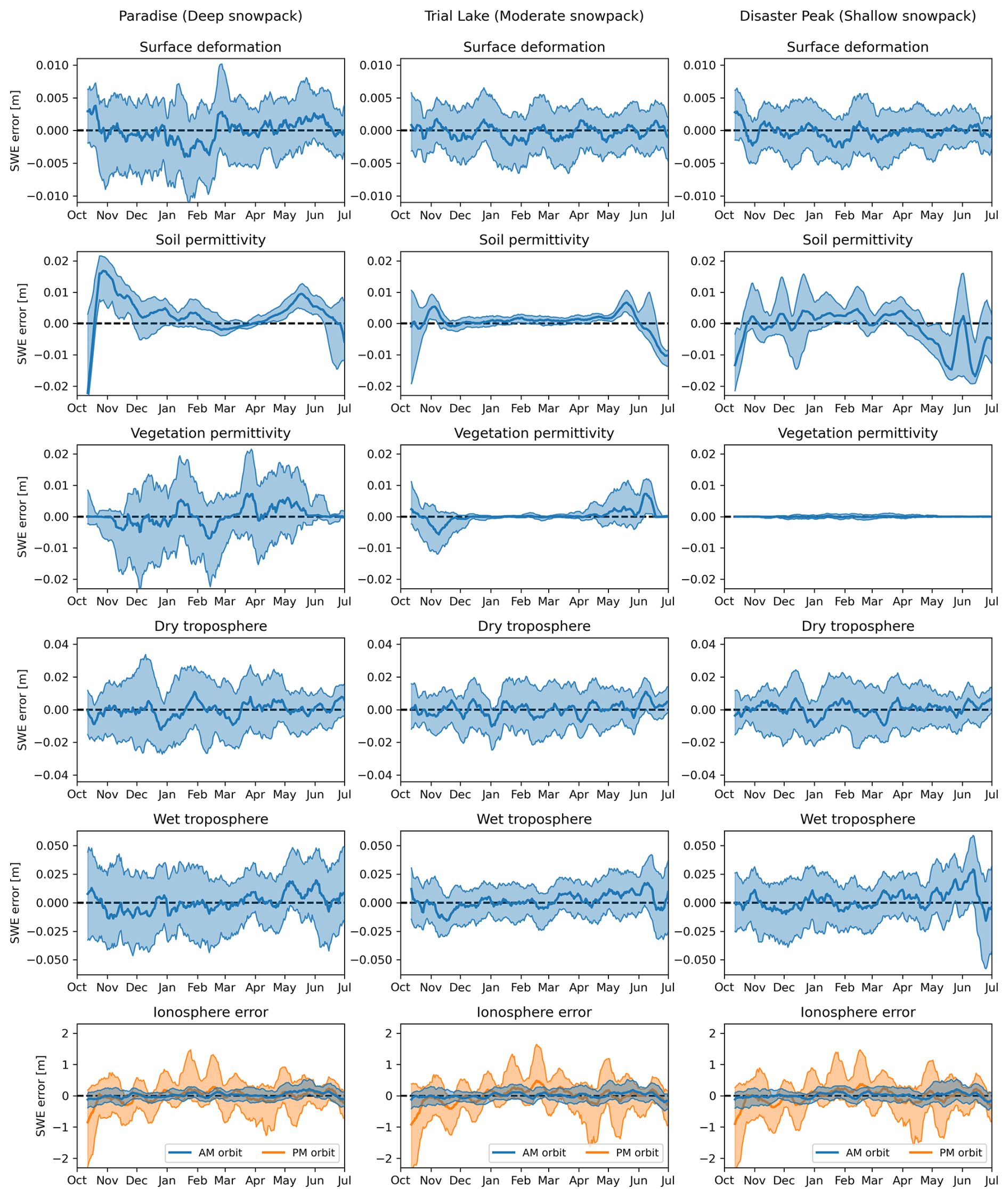
Figure 6 Non-snow error components at Paradise (left column), Trial Lake (middle column) and Disaster Peak (right column). In all subpanels the thick line shows the median value over water years 2016–2025 with shading between the interquartile range. Note the different y limits for different rows.

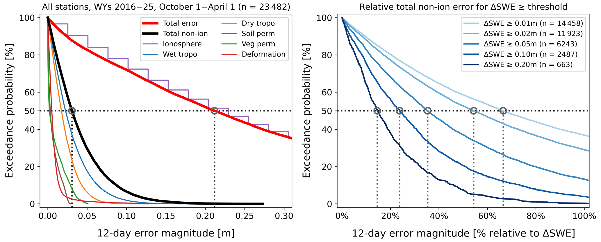
Figure 7 Exceedance probabilities for different non-snow errors. In both panels, the exceedance distributions are calculated using data from all stations (Table 2) for water years 2016–2025. Distributions in the left panel are calculated using 12 d errors from every day between 1 October and 1 April and presented as absolute values in units of meters. Note that the stepwise appearance of the ionospheric error (purple curve) is due to the relatively coarse precision of the IGS IONEX data (see Table 1). Distributions in the right panel are calculated from subsets of 12 d periods between 1 October and 1 April when ΔSWE was larger than the indicated threshold value (0.01, 0.02, 0.05, 0.1, and 0.2 m).

As indicated by the varying y axis limits between the rows, the range of absolute error values is smallest for surface deformation (top row) and increases down the rows. Note that all panels in a given row have the same y axis limits. Surface deformation errors do not show apparent seasonality at any of the three stations. The range of soil permittivity error (second row) is approximately double that of surface deformation error. At Paradise and (left column) and Trial Lake (middle column), soil permittivity errors are largest and most variable between October–December and May–July, with relatively small and consistent errors during the January–April. This reflects early season soil moisture changes from small accumulation and melt events with air temperatures near freezing, and late-season soil moisture changes due to snow melt. We note that errors from any non-snow factor in June and July are unlikely to affect InSAR SWE measurements at most locations because liquid water in the snowpack will have already rendered the technique impractical. Soil permittivity errors at Disaster Peak (right column) are more variable throughout the entire winter, which reflects the shallow snowpack and occasional mid-season melt events at this site. At all stations the soil permittivity error is positive for a majority of the season, which leads to the consistently positive cumulative errors shown in Fig. 3.

Vegetation permittivity errors (Fig. 6, third row) are influenced by canopy height and air temperature. The relatively large and variable vegetation permittivity errors throughout the season at Paradise are a result of tall vegetation (Table 2) and air temperatures that fluctuate both above and below freezing. In contrast, vegetation permittivity errors at Trial Lake show some variability in the early season but are consistently small between January and April as air temperatures become consistently cold. Vegetation permittivity errors at Disaster Peak are virtually zero because the surrounding shrub vegetation is only 0.5 m tall in the LANDFIRE canopy height dataset.

Error ranges for the dry and wet troposphere components (Fig. 6, fourth and fifth rows) are larger at all stations than those for surface deformation, soil permittivity, and vegetation permittivity components. At all stations the dry troposphere error fluctuates both above and below 0 and does not show pronounced seasonality. These patterns result in the small and fluctuating cumulative dry troposphere error shown in Fig. 3. The wet troposphere error does show some seasonal variation with generally negative values between October–March and generally positive values between April–July. These results indicate that wet troposphere effects are likely to negatively bias InSAR SWE measurements calculated from single nearest-neighbor interferograms during the majority of the accumulation season.

The ionosphere error (Fig. 6, bottom row) is the largest error component by two orders of magnitude. Accurate ΔSWE measurements using NISAR L-band data will not be possible unless ionospheric effects can be appropriately addressed. At all stations there is less ionospheric variability (and therefore less error variability) when the 12 d difference is calculated with morning observations instead of evening observations. For example, at Trial Lake, the seasonal average AM ionosphere error (mean of the middle AM orbit line) is 0.010 m with an average interquartile range (IQR) of 0.377 m. The seasonal average PM ionosphere error is 0.013 m with an average IQR of 1.031 m. The largest average difference between AM and PM errors is 0.312 m on 27 November, a critical early-season period when total SWE and ΔSWE are typically small. Ionosphere errors of 0.312 m potentially represent more than 100 % of the snowpack at many WUS locations in late November. The largest difference between AM and PM IQR is 1.206 m on 12 April, another critical monitoring period around the timing of peak SWE in the WUS. AM and PM results are similar at Paradise and Disaster Peak. For these reasons, we recommend using ascending NISAR overpasses to generate NISAR interferograms for ΔSWE measurements, which will acquire data at approximately 06:00 LT. However, depending on the area of interest, it may be the case that target locations are imaged only during descending overpasses (e.g., if a slope is within an area of radar shadow for the ascending overpass). Carefully accounting for ionosphere errors in these contexts will be critical for accurate interpretation of NISAR SWE measurements.

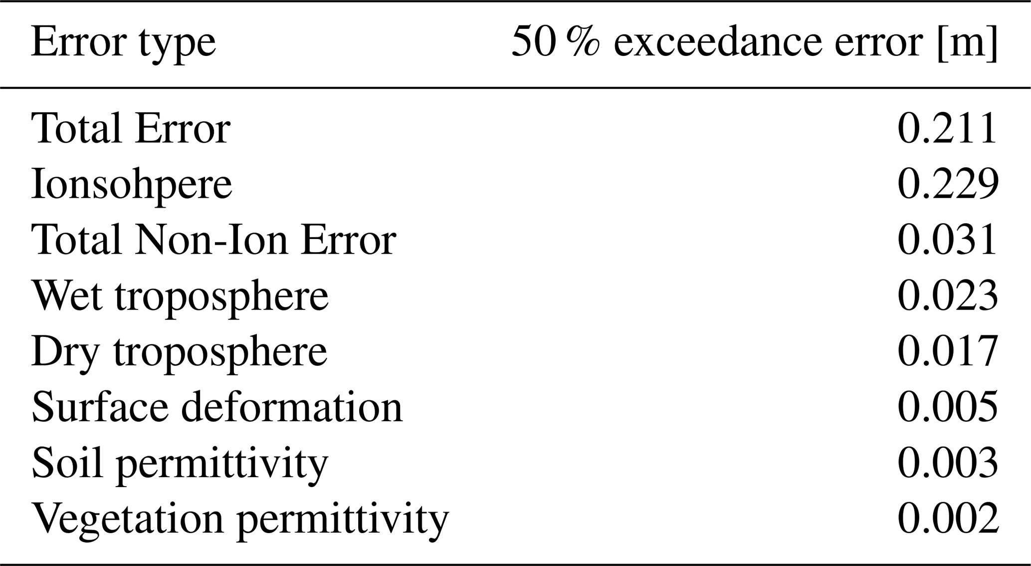
We summarize the non-snow errors over all 13 stations using error exceedance curves (Fig. 7), which show the probability of exceeding an error of a given magnitude if a single measurement is drawn at random from the distribution of all errors. All exceedance curves in the left panel of Fig. 7 were calculated using a combined timeseries of daily errors calculated between 1 October and 1 April for all water years at all stations (23 482 total measurements). For the western US stations we selected for this analysis, there is a 50 % chance that the total non-snow error present in any 12 d NISAR measurement is greater than 0.212 m (thick red line). If the ionosphere error is removed, the remaining non-ionospheric error (thick black line) will be greater than 0.031 m with 50 % probability. The 50 % exceedance error values for all curves are given in Table 4. Similar calculations for different probability thresholds can be done using the exceedance curves in the Fig. 7.

Table 4 50 % exceedance errors [m] for error curves shown in Fig. 7, left panel.

We used a similar analysis to investigate whether non-snow errors behave differently on days with vs. without a snow event. We split the 1 October through 1 April dataset into days where ΔSWE=0 (1784 total measurements) and days where ΔSWE≠0 (21 698 total measurements), representing both accumulation and ablation events. When ΔSWE=0, the 50 % exceedance thresholds were 0.210 m for total non-snow error and 0.031 m for non-ionospheric error. When ΔSWE≠0, the 50 % exceedance thresholds were 0.230 m for total non-snow error and 0.030 m for non-ionospheric error. The error curves for the two cases (not shown) were quite similar to those in the left panel of Fig. 7. This result indicates that non-snow factors affect the phase relatively consistently, regardless if a snow event occurs or not.

It is also important to consider the magnitudes of these errors relative to the real ΔSWE values measured at the stations during the same periods. To investigate snow events of varying magnitudes, we filtered our error dataset to select only measurements where the 12 d SWE accumulation at a given station was above a certain threshold (i.e., 0.01 m to include both small and large accumulations, or 0.2 m to isolate large accumulations only), then divided the total non-ionospheric errors from those periods by the accumulated SWE (Fig. 7, right panel). We removed the ionosphere error from this figure to improve clarity. The results indicate that for small SWE accumulations down to 0.01 m, there is a 50 % chance that the total non-ionospheric error present in a randomly selected NISAR measurement is greater than 67 % of the SWE accumulated during the same period. When we restrict the data to only consider large 12 d SWE accumulations (0.2 m or larger), the 50 % exceedance probability drops to 15 % of accumulated SWE. 12 d SWE accumulation events larger than 0.2 m were relatively rare in our dataset and occurred in less than 3 % of all 12 d periods.

Error variation over North American transects

With gridded datasets it is possible to assess how non-snow error components vary across larger regions, even if in situ stations are not available. Based on data availability we explore only the wet troposphere, dry troposphere, and morning/evening ionosphere errors between 2016–2025 across several transects in North America (Fig. 8). Over the North America S–N transect, the dry troposphere error becomes larger than the wet troposphere error north of approximately 63° latitude. Although the tropospheric errors in this region are only equivalent to several centimeters of SWE, the tundra snowpacks in northern Canada may only accumulate some tens of centimeters of SWE in a given season, and average ΔSWE is similarly small. Hence it remains important to account for both wet and dry troposphere effects when retrieving ΔSWE at high latitudes. We also note that the spatial correlation length of atmospheric pressure is on the order of hundreds of kilometers for atmospheric pressure, but is on the order of tens of kilometers for atmospheric water vapor. Therefore we expect that over a NISAR interferogram spanning hundreds of kilometers, the dry troposphere error may be relatively constant and vary primarily with topography but the wet troposphere error could vary horizontally over the scene. Correcting this wet troposphere effect will be critical, and potentially challenging, for accurate interpretation of spatially distributed ΔSWE measurements from NISAR.

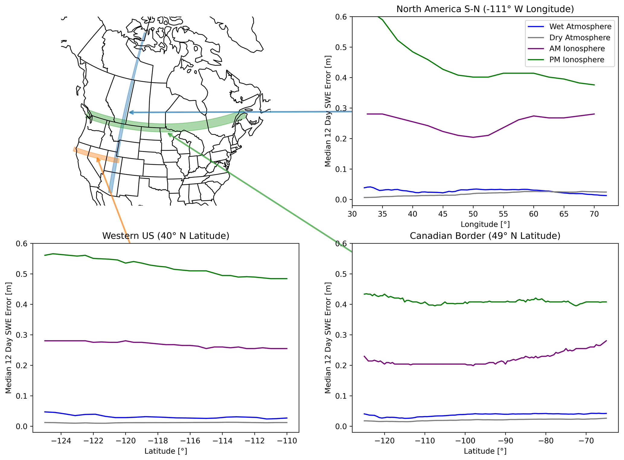
Figure 8 Spatial variation in wet atmospheric, dry atmospheric, and ionospheric errors across different transects in North America.

Similar to results from the SNOTEL stations, the average ionosphere error in the spatial transects is much larger than either the wet or dry troposphere errors. Decreases in errors in the middle of the North America S–N and Canadian Border transects are visible, indicating smaller 12 d ionospheric changes over the middle of the continent. However, even in these regions the ionospheric signal would dwarf expected values of ΔSWE in the same 12 d period. Regardless of location, there is less ionospheric variability (and therefore less error) when the 12 d difference is calculated with morning observations instead of evening observations (see Fig. 6). Therefore, for areas that fall within both ascending and descending overpasses, we again recommend using the ascending (morning) overpasses to generate NISAR interferograms for ΔSWE measurements. Morning overpasses also increase the probability of imaging dry snow during the transition from accumulation to melt season, which improves InSAR coherence and could potentially extend the measurement season by several weeks. For areas that fall only within descending overpasses, or if descending and ascending overpasses are used together to improve the temporal resolution of ΔSWE measurements, carefully addressing the ionosphere error will be crucial for accurate SWE measurement.

We are not aware of a daily, gridded soil moisture product that provides valid data during winter months. Based on the results of the SNOTEL analysis (Fig. 5, Table 3), soil permittivity errors have the greatest impact on shallow, low-elevation snowpacks with midwinter melt events or other factors leading to ephemeral snow. Although ephemeral and marginal snowpacks can play important ecological and climatological roles (Petersky and Harpold, 2018; López-Moreno et al., 2024), these snowpacks are less critical observation targets for current water resources applications in the western US. Measurements at high latitudes with intermittent frozen soils may see increased errors at the beginning of the accumulation season as soils go through freeze/thaw cycles, as this changes the penetration depth of the radar signals. We also note that changes in soil moisture are difficult to measure and interpret when soil temperatures are near freezing, which could further complicate soil effects on InSAR SWE measurements in permafrost regions.

5 Discussion

We analyzed the impact on SWE retrievals of five frequency-independent error sources and one frequency dependent (ionospheric) error source. For SWE measurements with L-band NISAR data, our analysis shows that the ionosphere, wet troposphere, and dry troposphere components have the largest error values for InSAR SWE retrievals across the western US (Fig. 7, Table 4). Fortunately, corrections for these three errors are planned for NISAR standard interferogram products (Brancato et al., 2024), which will ultimately improve the accuracy of ΔSWE retrievals from a single interferogram. However, it is important to consider the offsetting effects of different error components when the total SWE is calculated by integrating a timeseries of ΔSWE measurements. At many stations, the cumulative wet and dry troposphere errors introduced negative bias into 1 April SWE measurements while soil moisture errors introduced a positive bias on average over the 10 year period investigated (Fig. 5). Removing only the troposphere errors may actually decrease the overall accuracy of the 1 April SWE measurements at those locations. For some locations with moderate to deep snowpacks, it may be better to leave all non-ionospheric errors present in ΔSWE calculations, assuming a sufficiently long integration time.

Another consideration for troposphere corrections in NISAR standard interferograms is the length scales at which the corrections are calculated and applied. Atmospheric pressure may have a correlation length approaching 100 kilometers, approximately the size of a satellite tile. However, the correlation length of atmospheric water vapor is smaller than that of pressure: at horizontal spatial scales less than 6 km, atmospheric water vapor is well-approximated by Gaussian random fields (Calbet et al., 2022). Hence, temporal changes in atmospheric water vapor may add unbiased spatially variable random errors to InSAR SWE measurements over a basin of interest, while temporal changes in atmospheric pressure may add overall bias to measurements over the same region. But this assumes that the atmospheric models used to calculate the corrective layers can accurately represent atmospheric spatial variability in complex terrain. If the models are too coarse to simulate relevant atmospheric processes over mountainous regions, significant troposphere effects may still be present in phase measurements even after an attempted correction. This may complicate the interpretation of ΔSWE measurements from a single interferogram, especially in complex terrain where snow depth can have a correlation length in the tens of meters (Blöschl, 1999). Future work to examine atmospheric errors in NISAR SWE measurements could involve reprocessing Level 1 data with higher resolution weather models (e.g., HRRR over the western US) and exploring time-series inversion approaches.

Efforts to estimate SWE from NISAR in other regions should carefully consider all error components based on site-specific characteristics. In some environments it is possible that some non-snow error factors are correlated. For example, measurements at high latitudes may be particularly influenced by surface deformation caused by freezing and thawing soils, which may also increase soil permittivity errors early in the accumulation season. Additionally, we note that sensor-specific factors may affect InSAR SWE measurements to a greater degree than the error components discussed here. We did not consider temporal coherence of InSAR phase, which is a function of incidence angle as well as changes in surface characteristics (Zebker and Villasenor, 1992; Rosen et al., 2000). In particular, although vegetation permittivity errors were small at most stations (Figs. 5 and 7), InSAR SWE measurements are not possible over sufficiently dense forest cover due to high temporal decorrelation; previous work has shown SWE retrievals possible for forest cover fractions less than 0.5 (Bonnell et al., 2024b). These and other sensor-specific factors (e.g., radar shadow) must be considered alongside the non-snow error components discussed here.

We note several limitations of our analysis. First, this work focused on the simplest time series approach using cumulative nearest-neighbor interferograms. We do not attempt to explore the improvements from more complex time-series approaches like small-baseline subset analysis (Li et al., 2022) or phase-linking (Eppler and Rabus, 2022) to separate systematic signals of interest from temporally random fluctuations in atmospheric phase. If applied carefully, more advanced InSAR methods have the potential to significantly reduce non-snow errors compared to a nearest-neighbor approach. Next, there is considerable range in the spatial resolution and fidelity of the datasets we used to calculate non-snow errors. For example, soil moisture measurements came from point-based, high fidelity instruments while the data relevant for ionosphere and troposphere errors came from coarse reanalysis products that contain larger errors and biases. Future work with other data sources such as radiosondes for troposphere changes and multi-frequency SAR systems for the ionosphere would be valuable.

Finally, this work could be expanded both spatially and temporally. We analyzed errors at only 13 SNOTEL stations across the WUS. Although this selection was partially dictated by data availability (see Sect. 2.3), it is possible that our results would change if we had selected different sites. For example, two of our three shallow snowpack stations (Disaster Peak and Quemazon) are in post-burn areas and may have snow accumulation and melt dynamics that are not fully representative of their broader geographic regions (Smoot and Gleason, 2021). However, our intent is not to draw broad conclusions about the method based on the 13 sites selected; rather, we aim to illustrate that the non-snow factors we considered here can have different magnitudes and effects in different snowpacks. Especially given that wildfire area has been increasing in snow-dominated regions across the WUS since the 1980s (Kampf et al., 2022) and WUS snowpacks are projected to continue their general decline (Siirila-Woodburn et al., 2021), it is likely that the WUS will become more reliant on shallow and post-burn snowpacks for water resources in the coming years and decades. We encourage future work in snow remote sensing to continue examining shallow and marginal snowpacks (López-Moreno et al., 2024). More broadly, a future global scale analysis would be useful in capturing the variability of each component in a larger diversity of ecoregions, including regions with more frequent large accumulation events. We did not evaluate the error associated with very large SWE changes that would cause phase wrapping (ΔSWE≥0.2385 m), as this would require evaluation of the impact of various phase unwrapping algorithms beyond the scope of this study. We note that 12 d ΔSWE≥0.2385 m was only recorded 418 times in our dataset, approximately 1.8 % of observations. Expanding the analysis with a longer temporal record would better capture ionospheric cycles which occur on the order of years to decades.

6 Conclusions

We simulated errors in six non-snow components (ionosphere, wet troposphere, dry troposphere, soil permittivity, vegetation permittivity, and surface deformation) for SWE measurements derived from L-band (1.257 GHz) InSAR measurements at a 12 d measurement frequency, based on the NISAR data acquisition strategy over the western US. We compared the non-snow errors to SWE measured at 13 SNOTEL stations spanning a range of snow and environmental characteristics (Table 2). Temporal variation of total electron content in the ionosphere causes the largest non-snow error by an order of magnitude, with 50 % of measured 12 d errors exceeding 0.229 m or 463 % of measured ΔSWE (when ΔSWE≥0.01 m) over the same periods (Table 4, Fig. 7). When ionosphere errors are removed, the 50 % exceedance probability of remaining non-snow error is reduced to 0.031 m or 67 % of ΔSWE. The wet and dry troposphere errors, due to temporal variation in atmospheric water vapor and pressure, respectively, are the largest non-ionospheric components, followed by surface deformation, vegetation permittivity, soil permittivity.

When a timeseries of 12 d ΔSWE measurements is integrated to obtain seasonal SWE accumulation, the cumulative effects of non-snow errors partially offset each other (Fig. 5). At most stations, cumulative soil permittivity errors introduce a positive bias into 1 April SWE measurements, while cumulative troposphere errors introduce a negative bias. The net result is that at 10 of 13 SNOTEL stations, the total cumulative error for all non-ionospheric components is within 10 % of measured 1 April SWE (Table 3), meeting accuracy targets for remotely sensed SWE measurements established in the 2017–2027 National Academies Decadal Survey. The three stations where errors exceeded 10 % of 1 April SWE represent shallow snowpacks (average 1 April SWE between 0.060–0.308 m) and in two cases, post-burn areas. However, the cumulative ionosphere error at all stations ranged between 16 %–670 % of 1 April SWE, well outside the target accuracy threshold.

The importance and challenge of accounting for all of these error sources, including evaluating the uncertainty in the corrections, demonstrates the necessity for independent calibration and validation from in situ stations and field efforts. InSAR SWE estimates will not produce spatially and temporally complete information, since NISAR has a 12 d orbit cycle and the technique will not work in all locations at all times (i.e., in dense forests or wet snowpacks). A data assimilation approach that uses InSAR SWE estimates and in situ observations to correct a physically-based snowpack model will likely provide the most robust SWE estimates.

For future work that makes use of NISAR-derived SWE measurements, we make the following suggestions:

• Careful removal of ionospheric effects from phase data is critical for accurate SWE measurements from NISAR, both for 12 d ΔSWE and season-long accumulation. If possible, use interferograms generated from ascending (morning) NISAR acquisitions to reduce ionospheric error and improve chances of imaging dry snow.

• Wet and dry troposphere errors must be removed for accurate ΔSWE measurements from a single NISAR interferogram. This is especially relevant for interpreting spatial patterns of snow accumulation at basin to range scales. Removing errors from surface deformation, vegetation permittivity, and soil permittivity will also improve accuracy but are less critical.

• Removing non-ionospheric error components from cumulative measurements requires careful consideration. Integrated errors between 1 October and 1 April had offsetting effects for different components (e.g., soil permittivity and wet troposphere); removing a single component without its offsetting effect may actually decrease the accuracy of accumulated SWE measurements. Future work should examine how these offsetting effects change over varying integration periods, as well as the interannual variation of these relationships.

• Site-specific factors should be considered to identify more or less influential error sources. For example, surface deformation may be more important to correct for SWE measurements over permafrost than over the non-frozen soils we considered here.

• Although we could not consider sensor-specific factors like temporal coherence, radar shadow, or phase unwrapping in this analysis, they may introduce more error into NISAR SWE measurements than some of the components we discussed here.

• Removing non-snow errors may be more feasible using more complex InSAR data processing algorithms, including small-baseline subset analysis or phase-linking.