Scale patterns of the Sentinel-1 SAR-based snow depth product compared with station measurements and airborne LiDAR observations

Water storage in snowpacks in mountainous areas is critical for hydropower production, hydrological forecasting, and freshwater availability. Spaceborne synthetic aperture radar (SAR) is a powerful tool for quantitatively measuring snow mass because of its high spatial resolution and signal sensitivity to snow depth (SD). In particular, the first SAR SD product (C-snow) based on Sentinel-1 satellites displays high sensitivity to depolarization signals for dynamic SD monitoring in mountainous areas. Moreover, upscaled C-snow retrievals (e.g., 10 and 25 km) have been used to provide reference data to train machine learning models, improve passive microwave-based retrieval, and calibrate many hydrological models. However, to date, a systematic assessment of C-snow products at various scales has not been conducted. In this study, the performance of C-snow products at three scales (1, 10 and 25 km) is compared via station-based measurements and airborne LiDAR observations, and the scale patterns associated with the heterogeneity of the geographic environment and the representativeness of so-called true data are analyzed. The scale patterns of C-snow products vary across resolutions. They differ from the patterns observed in the station and airborne reference data. As the spatial scale increases from 1 to 25 km, the error of C-snow retrieval in reference to station measurements tends to increase (e.g., ubRMSE from 69.43 to 81.87 cm; bias from −8.89 to 11.66 cm), whereas it tends to decrease compared with Airborne Snow Observatory (ASO) data, with ubRMSE values ranging from 104.3 to 83.29 cm and bias values ranging from −91.31 to −52.73 cm. We also found that land cover types, e.g., tree cover and permanent ice, affect the C-snow product at various scales. Overestimation tends to occur in coarse pixels covered with even a small amount of permanent ice. The findings indicate that C-snow retrieval at three scales is characterized by high uncertainty. Therefore, researchers should focus on developing a robust SD retrieval algorithm by combining SAR backscattering signals and polarimetric and interferometric information.

1 Introduction

Snow storage and seasonal meltwater in mountains are components of the “water towers” that form in mountainous areas globally. Therefore, quantitatively estimating snow mass in mountainous areas is very important for hydropower production, hydrological forecasting, and freshwater availability (Barnett et al., 2005; Dozier et al., 2016; Daloz et al., 2020; Qin et al., 2020). The snow water equivalent (SWE) is a parameter that reflects how much water the snowpack contains and can typically be estimated from snow depth (SD) and snow density. Satellite remote sensing has been demonstrated to be an effective tool for monitoring multiscale SD information, which enhances our understanding of water availability in snowpacks (Chang et al., 1987; Kelly, 2009; Takala et al., 2011; Lievens et al., 2019).

Conventional SD monitoring methods, such as manual field measurements and ground station observations, can provide accurate local data but are difficult to implement in remote mountainous areas with complex terrain. Microwave remote sensing is the most widely used technology for retrieving SWE because of its ability to penetrate snowpack and the volume scattering effects caused by snow particles (Chang et al., 1987; Tsang et al., 2022). While passive microwave remote sensing (e.g., radiometer-based methods) is typically employed, its coarse spatial resolution (∼ 25 km) limits its ability to capture fine-scale spatiotemporal variability in snowpack properties, particularly in complex mountainous terrain. In general, active microwave remote sensing, especially synthetic aperture radar (SAR), has advantages over passive microwave techniques for characterizing the SWE across high-mountain regions (Dozier et al., 2016). Notably, compared with passive microwave remote sensing (dozens of kilometers), spaceborne SAR can support fine-spatial-resolution (dozens of meters) monitoring. The snowpack in mountainous areas is typically deep (up to one or several meters), and the evolution of snowpack in these areas is generally much more complex than that in flat areas. For example, the snow density typically ranges from 100 to 550 kg m⁻³ for seasonal snow (Sturm et al., 2010). Owing to snowfall accumulation and prolonged wind- and gravity-driven compaction, it can reach 550–700 kg m⁻³ (Lemmetyinen et al., 2016; Venäläinen et al., 2021). In addition, owing to the large negative temperature gradient between the air temperature and ground temperature, the development of depth hoars is common (Fierz et al., 2009). For example, the snow grain size in depth hoars can reach the centimeter level at high elevations and on shady slopes (King et al., 2018; Picard et al., 2022). Thus, the signals of typically used frequencies (e.g., the Ka band) in passive microwave remote sensing tend to be saturated within the SD range of 40–80 cm (Derksen et al., 2010; Takala et al., 2011; Picard et al., 2018).

In recent years, the scientific community has increasingly focused on monitoring the SWE in mountain regions using C-band SAR observations because of their strong penetration depth and data accessibility. Early studies on C-band SAR for SD estimation were limited primarily to shallow snow environments outside mountainous regions and co-polarization measurements, which showed limited sensitivity to dry snow conditions (Bernier et al., 1999; Shi and Dozier, 2000). Theoretical advances in microwave scattering models (Ulaby et al., 1982; Chang et al., 2014) have improved the understanding of snowpack interactions with C-band signals. Notably, although snow volume scattering is stronger in high-frequency Ku-bands than in other bands (e.g., X-, C, or L-band) in theory, the sensitivity of the backscattering coefficient at this frequency is also limited to approximately 150 cm (Rott et al., 2010; Cui et al., 2016; Zhu et al., 2021). Moreover, Lievens et al. (2019) observed the sensitivity of the depolarization signal (cross-polarization ratio VH $/$ VV) in the C-band to the SD and innovatively developed a C-band-based SD retrieval algorithm for mountains in the Northern Hemisphere. In particular, the backscattering coefficient at cross-polarization is more sensitive to volume scattering than co-polarization is because of the anisotropic nature of snow grains (Du et al., 2010; Chang et al., 2014; Leinss et al., 2016), and this physical mechanism is used for SD retrieval; in addition, co-polarized and cross-polarized signals are similar for surface scattering at the snow–soil boundary (Shi and Dozier, 2000; Lievens et al., 2022; Borah et al., 2024). Thus, the ratio of cross-polarized to co-polarized signals increases snow volume scattering and weakens surface scattering between snow and soil.

The C-snow product provided SD retrievals at a 1 km resolution without wet snow masking (Lievens et al., 2019). It reported a temporal correlation ranging from 0.65 to 0.77 and a mean absolute error of 0.18–0.31 m. Given its high resolution of 1 km, the C-snow product can potentially be used to assess the heterogeneity of snow distribution in mountainous areas (Alfieri et al., 2022; Girotto et al., 2024). However, to date, it has only been evaluated from the point to regional scales and not at the global scale. For example, an evaluation across the Po River Basin in Italy revealed that the RMSE ranges from 20 to 60 cm in reference to ultrasonic sensor measurements (Alfieri et al., 2022). Sourp et al. (2025) compared C-snow retrieval products with the results of airborne LiDAR surveys in the Sierra Nevada region from 2017–2019 and reported that the RMSE ranged from 21 to 138 cm and that the bias reached −124 cm. Hoppinen et al. (2024) evaluated algorithm performance at six study sites across the western United States (US) using airborne LiDAR observations collected during the winters of 2019–2020 and 2020–2021, with mean RMSE and bias values of 92 and −49 cm, respectively. In addition, C-snow SD data at 10 and 25 km resolutions, which are derived from the 1 km C-snow product, have been used as reference datasets for training machine learning models to improve passive microwave SWE estimates (Xiong et al., 2022; Yang et al., 2024). Lievens et al. (2022) employed Sentinel-1 backscatter observations to retrieve SD across multiple spatial resolutions in the European Alps and evaluated the retrieval performance. Compared with the performance at the 500 m and 1 km resolutions (by linearly averaging the 100 m retrievals), the performance at the 100 m resolution slightly decreased because of the impacts of radar speckle noise, geometric distortions, and local heterogeneity in topography, land surface properties, and snow characteristics.

High-resolution SD data at 1 km are suitable for hydrological modeling and snow disaster monitoring (Wan et al., 2022). SD data at a 10 km resolution are appropriate for operational environmental prediction, hydrological forecasting and seasonal forecasting at regional scales (Alonso-González et al., 2018), whereas 25 km resolution data are widely used for SD monitoring, climate change analysis, and model evaluation at global and regional scales (Tanniru and Ramsankaran, 2023). The accuracy of the C-snow product at 1, 10 and 25 km still requires further investigation. The scale effect across three spatial resolutions and sensitive influencing factors (e.g., topography, land cover and wet snow) are crucial to consider when evaluating the performance of the C-snow product. However, exploration of these factors remains insufficient, thus hindering our understanding of ways to improve C-band SD retrieval technology.

Therefore, the specific objectives of our study are to (1) systematically evaluate the error of the C-snow retrieval across 1, 10 and 25 km spatial scales via both station-based measurements and airborne LiDAR data and analyze the sensitivity of the error to various factors, as well as (2) quantitatively compare the scale patterns of the SD products at three spatial scales and explain the inconsistency of scale effects on the basis of different reference datasets (stations vs. Airborne Snow Observatory, ASO). To achieve this goal, we used measurements from point-scale stations and airborne LiDAR campaigns. The latter provides spatially extensive SD mapping, which is more extensive than that provided by station data, and its coverage remains within the western US, whereas the station data are valuable for characterizing the SD distribution and assessing snow heterogeneity. This paper is structured into five sections. Section 2 describes the methods and data. The results and discussion are presented in Sects. 3 and 4, respectively. Finally, Sect. 5 presents the conclusions, and future research is discussed.

2 Data and Methodology

2.1 Sentinel-1 SD product

The first 1 km SD product based on C-band SAR, covering all mountain ranges in the Northern Hemisphere, was developed by Lievens et al. (2019). The dataset is publicly available through the C-SNOW project. An empirical change detection method is used to retrieve the SD (Lievens et al., 2019). The available C-snow dataset covers the period from 1 September 2016 to 19 May 2019. The spatial resolution of the C-snow product is 1 km, and the temporal resolution varies from daily to every two weeks, depending on the frequency of Sentinel-1 observations.

2.2 Reference SD data

2.2.1 Station-based measurements

In this study, we collected six station-based observational datasets as reference data to evaluate and compare the performance of the C-snow product across three scales (Fig. 1a). They include the Global Historical Climate Network (GHCN), Canadian Historical Snow Water Equivalent (CanSWE), in situ measurements from Chinese weather stations (China-SD), SD measurements from Maine (Maine-SD), SD variables from Snow Telemetry (SNOTEL) and an SWE dataset in the range of the former Soviet Union (Russia-SWE). For the Russia-SWE datasets, we used a fixed snow density of 0.24 g cm⁻³ to convert the SWE to the SD (Takala et al., 2011; Luojus et al., 2021).

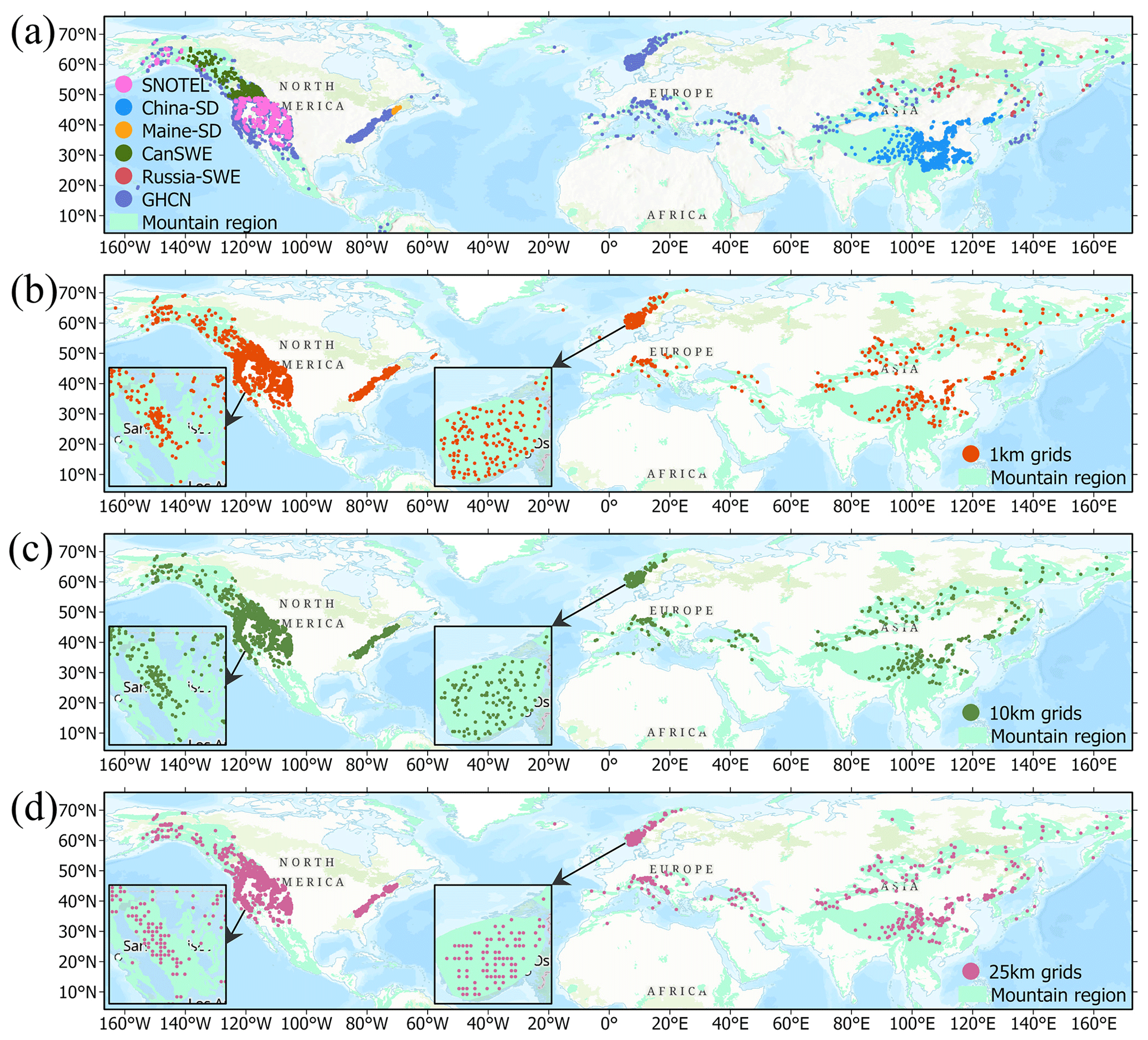
Figure 1 Spatial distribution of (a) stations in various SD datasets and of the matched grids at the (b) 1 km, (c) 10 km, and (d) 25 km scales. Zoomed-in views show the detailed distributions of grid locations in the Sierra Nevada range over the US and the Jotunheimen mountain range in Norway and Sweden. Base map sources: Esri, TomTom, Garmin, FAO, NOAA, USGS, EPA, USFWS.

The station-based observations span multiple regions and stations. The CanSWE dataset from Canada includes data from 273 stations in mountainous regions and can be accessed via https://doi.org/10.5281/zenodo.5217044 (Vionnet et al., 2021b, a). The GHCN dataset includes data from 4133 stations in mountainous regions and provides SD values worldwide (Menne et al., 2012; available at ftp://ftp.ncdc.noaa.gov/pub/data/ghcn/daily/, last access: 18 November 2025). The China-SD dataset from the China Meteorology Administration (http://data.cma.cn/, last access: 18 November 2025) includes observations from 744 stations in mountainous regions. The SNOTEL dataset was acquired from 677 stations in mountainous regions in the US (Serreze et al., 1999; available at https://toolkit.climate.gov/tool/snow-telemetry-snotel-data-viewer, last access: 18 November 2025). The Russia-SWE dataset from former Soviet Union regions contains observations from 52 stations in mountainous regions (Bulygina et al., 2011), and it can be downloaded from the All-Russia Research Institute of Hydrometeorological Information–World Data Center (http://meteo.ru/, last access: 18 November 2025). Additionally, the Maine-SD dataset for the Maine region includes information from 92 stations in mountainous regions; it can be accessed via Maine Geological Survey Data (https://mgs-maine.opendata.arcgis.com, last access: 18 November 2025).

To control the quality of the station observations, we excluded observations with an SD of zero and then removed outliers using the interquartile range (IQR) method, where observations were classified as outliers if they fell outside the range [$Q\mathrm{1}-\mathrm{1.5}\times \mathrm{IQR}$, $Q\mathrm{3}+\mathrm{1.5}\times \mathrm{IQR}$]. Here, Q1 represents the 25th percentile, Q3 represents the 75th percentile, and IQR is calculated as Q3−Q1. This filtering was performed separately for each station to account for differences in data distribution across locations. Finally, we excluded stations with fewer than three SD measurements over the entire study period. Later, we calculated the averages of measurements from multiple stations within pixels at the scales of 1, 10 and 25 km (see details in Sect. 2.4). Figure 1b–d show the processed grids of the SD as the reference datasets at the 1, 10 and 25 km scales in the two selected areas; the number of grids decreases from 2838 to 2223 and to 1500 grids as the scale increases.

2.2.2 ASO data

The ASO data provide high-resolution, spatially comprehensive measurements of SD, SWE, and snow albedo in mountain basins by combining airborne lidar, imaging spectrometry, and physically-based snow modeling (Painter et al., 2016). Airborne remote sensing campaigns over the western US were conducted from 2013 to the present, and hyperspectral reflectance and LiDAR SD data were collected in Colorado, California, Oregon, and Washington. These data are used to develop standard basin-scale instantaneous SD maps, with a resolution of 3 m and an evaluated accuracy of 0.08 m (Painter et al., 2016). The ASO SD is calculated using scanning LiDAR measurements, a straightforward and robust approach involving the subtraction of snow-free surface elevation data from snowpack surface elevation data. To assess and compare the accuracy of the C-snow product at different scales, we obtained 59 ASO maps (within California and Colorado) at a 3 m resolution from September 2016 to May 2019. Figure 2 provides the statistics of the available measurements by basin and date.

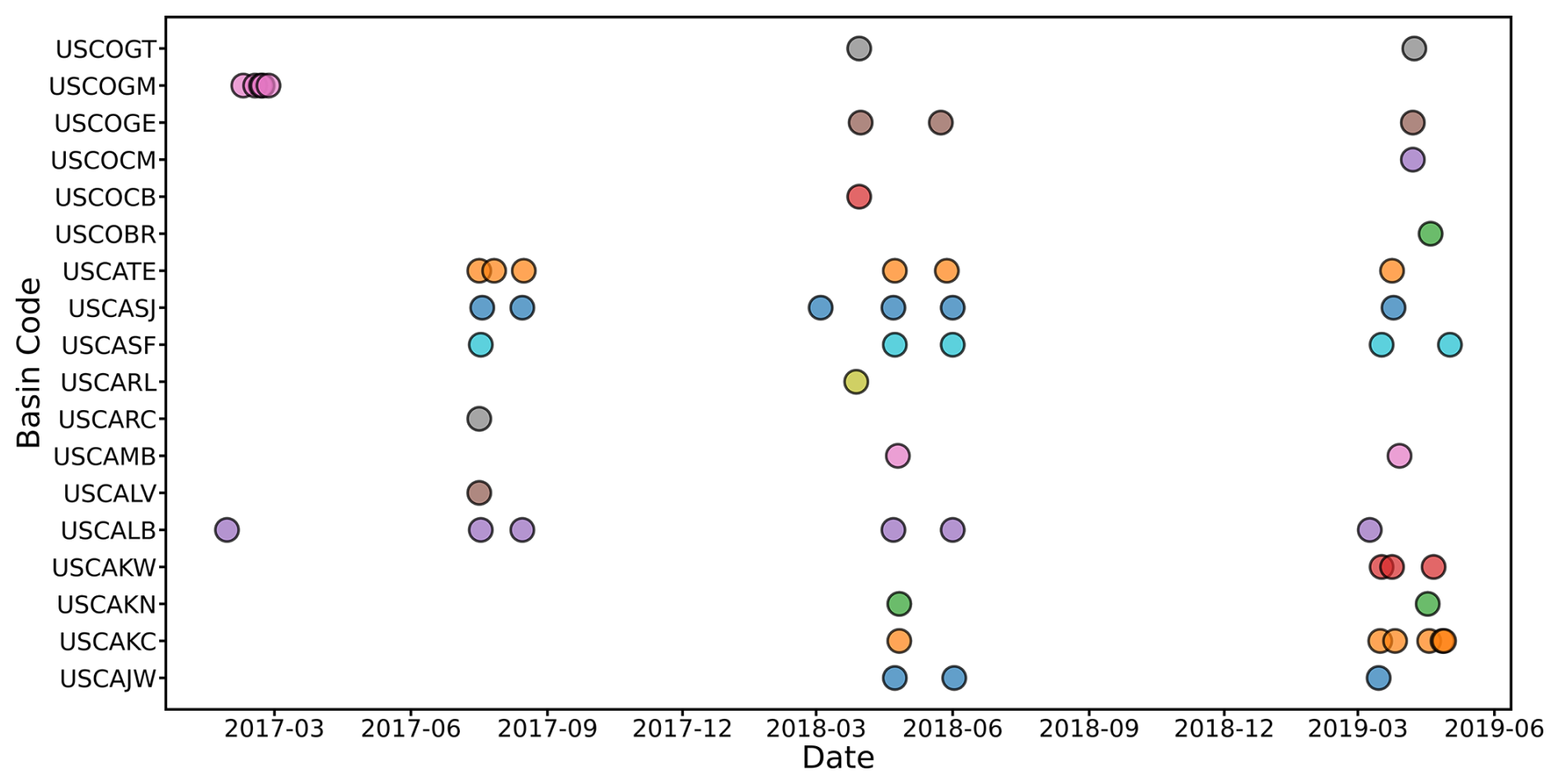
Figure 2 Temporal distribution of the ASO observations used in this study. The markers with different colors represent different basins.

2.3 Auxiliary data

To evaluate the influence of land cover type, forest fraction, and topography (elevation and its standard deviation) on the accuracy of C-snow SD, we collected auxiliary datasets (Table 1) from the Google Earth Engine and processed them at various scales (1, 10, and 25 km). The land cover data used in this study are from the ESA WorldCover 10 m 2020 product, which includes 11 land cover types: tree cover, shrubland, grassland, cropland, built-up, bare or sparse vegetation, snow and ice, permanent water bodies, herbaceous wetland, mangroves, moss and lichen. In this study, the tree cover type is labeled “tree cover”, the snow and ice types are labeled “permanent ice”, and all the remaining types are labeled “other type”.

Table 1 Description of the auxiliary data used in this study.

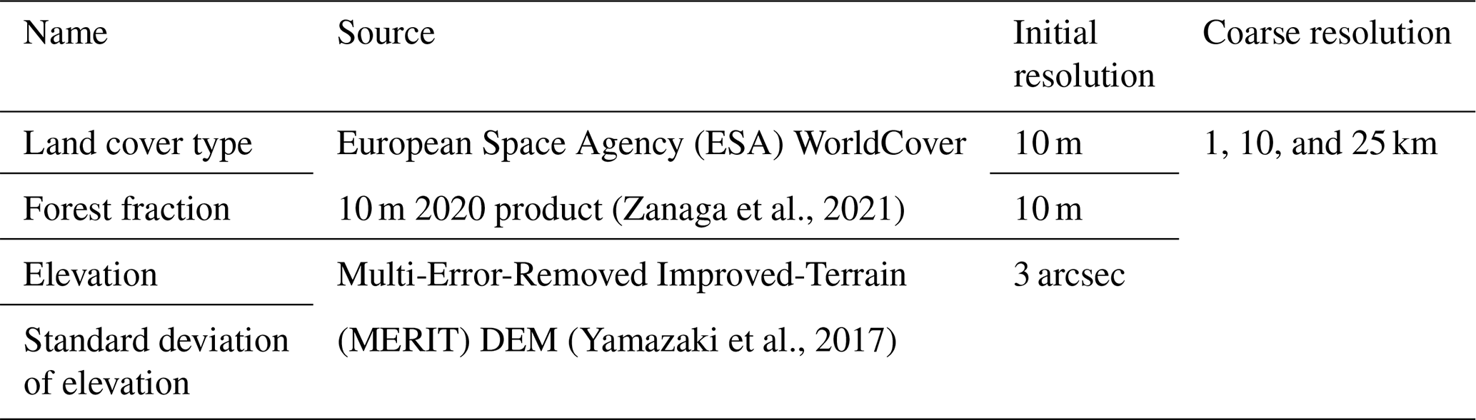
To match the scales of the C-snow SD data, we resampled the auxiliary data accordingly. The land cover type data were first resampled to a 1 km resolution via the mode resampling method. These 1 km land cover data were subsequently further resampled to 10 and 25 km resolutions. During the resampling process, if a certain land cover type occupied 80 % or more of a large grid of 10 or 25 km, that type was then assigned to the resampled grid; otherwise, no land cover type was assigned. The forest fraction, elevation, and standard deviation of the elevation at a 1 km resolution were resampled to 10 and 25 km resolutions via the average resampling method.

2.4 Methodology

Figure 3 shows the workflow of this study. To assess the accuracy of C-snow retrieval at different scales, the 1 km C-snow product was resampled to 10 and 25 km. Here, we directly used the mean resampling method according to previous studies (Broxton et al., 2024; Herbert et al., 2024). Moreover, we tested and compared the mean and median sampling methods and obtained similar validation results. To control equality and the representativeness of coarse-resolution pixels, we selected only the 10 and 25 km grids in which the percentage of the snow-covered area was at least 80 %. The average 1 km SD values within the coarse-resolution pixels were then used as the 10 or 25 km-scale products (Fig. 3). To compare C-snow with station-based data and ASO observations at different scales, we also resampled the 3 m-resolution ASO data to 1, 10, and 25 km. When the ASO data were resampled, we calculated only the average for grids for which the number of 3 m ASO observations at larger scales (1, 10, and 25 km) was not less than 30 %. Here, we selected 30 % to ensure a sufficient quantity and representativeness of the validation samples.

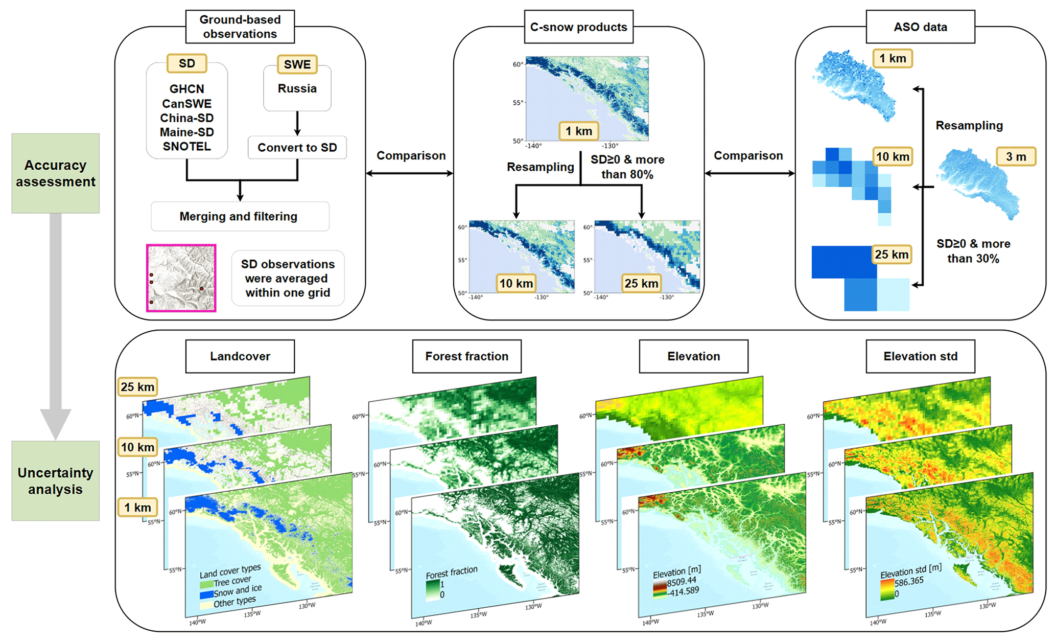
Figure 3 Diagram of the research workflow. Basemap sources: Esri, TomTom, Garmin, FAO, NOAA, USGS, EPA, USFWS, NRCan, Parks Canada, State of Alaska.

Additionally, we explored the relationships between the land cover type, forest fraction, elevation and standard deviation of the elevation and the C-snow SD across different scales. The difference in elevation between the station and the corresponding grid was computed by subtracting the grid elevation from the station elevation. Four evaluation metrics were used to assess the C-snow products: the Pearson correlation coefficient (corr.coe), bias, unbiased root mean square error (ubRMSE), and relative bias (Rbias).

3 Results

3.1 Comparison of the SD retrieval results with station-based measurements and ASO LiDAR data

We evaluated the C-snow SD retrievals through comparisons with station-based measurements across different spatial scales. Figure 4 displays a comparison of the station measurements and the C-snow products at different scales. As the scale increases, corr.coe decreases from 0.52 to 0.32. Additionally, ubRMSE increases from 69.43 to 81.87 cm, reflecting increased uncertainty. Moreover, as the scale increases, the mean bias shifts from a slight underestimation of −8.89 cm to a slight overestimation of 11.66 cm. The decreased correlation is reasonable because the station observations are point-scale measurements. Even for pixels with multiple stations, it is difficult to obtain a continuously distributed SD map using a limited number of samples.

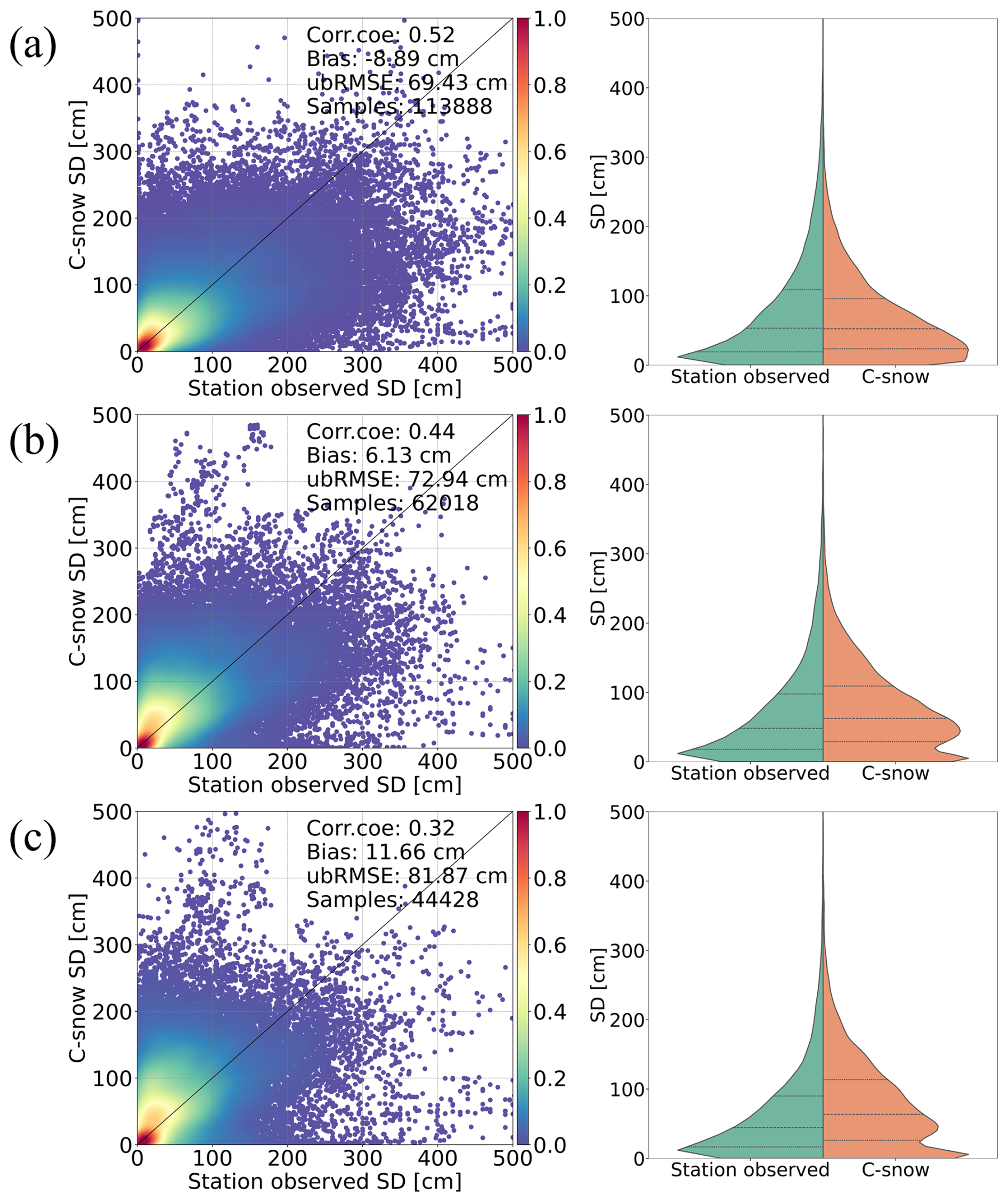
Figure 4 Comparisons (left column) and distributions (right column) between the C-snow SD and the station-observed SD at (a) 1 km, (b) 10 km, and (c) 25 km scales. The dashed lines in the right column indicate the 25th, 50th and 75th percentiles.

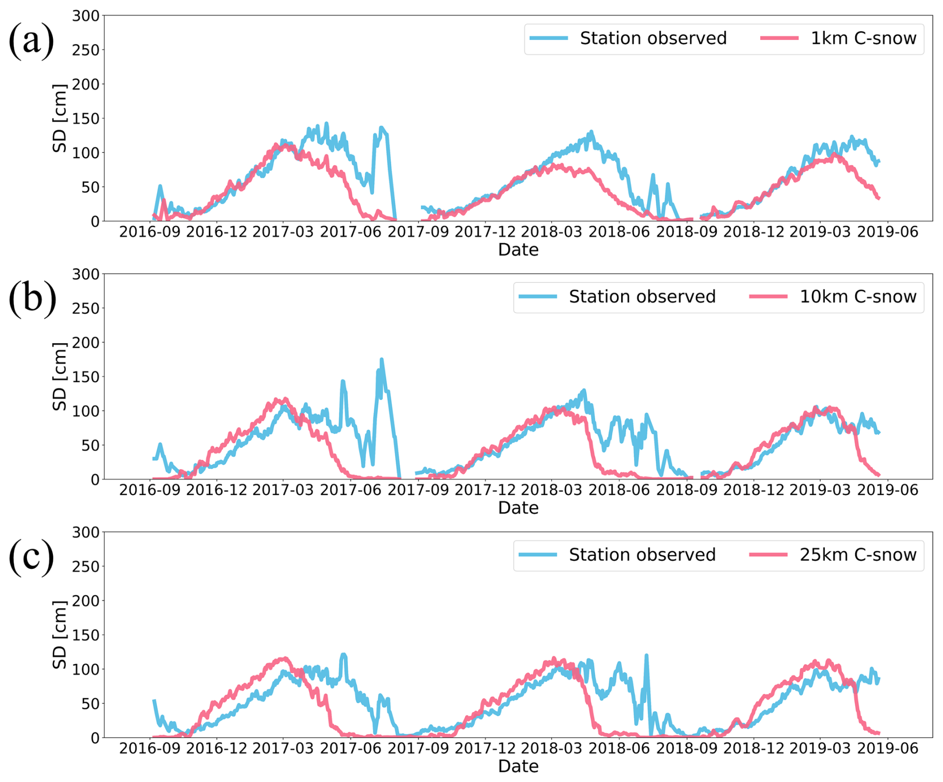
Figure 5 Average weekly SD time series of stations and corresponding C-snow grids at (a) 1 km, (b) 10 km, and (c) 25 km resolution across the mountainous regions of the Northern Hemisphere.

Figure 5 shows the average time series of the C-snow products compared with the station measurements. In general, at all scales, the C-snow SD is underestimated in the snowmelt season starting in March. As the spatial scale increases from 1 to 25 km, both the magnitude and duration of the discrepancies between C-snow and station SDs increase. Specifically, the average SD from the stations becomes increasingly greater than the C-snow SD during the dry snow season and increasingly lower during the melt season. This explains the decreased correlation between the two datasets as the scale increases in terms of temporal variation. The underestimation of the SD for C-snow at 1 km in the wet snow season can be explained as the damping effect of liquid water on microwaves. The differences at 25 km are more difficult to explain. This is because a long snow season is usually associated with a high SD. Therefore, this pattern makes it difficult to provide a consistent answer that explains why the stations are characterized by lower SD during the dry snow season and higher SD during the wet snow season. To explore this question, we must assess the relevant spatially distributed influential factors.

The C-snow retrieval results are assessed at different scales on the basis of the ASO data (Fig. 6). At the 1 km scale, the C-snow SD is underestimated, with a bias value of −91.31 cm and an ubRMSE as high as 104.3 cm. As the scale increases, the accuracy of C-snow increases, with the ubRMSE decreasing from 104.30 to 83.21 cm and the bias decreasing from −91.31 to −52.73 cm. Overall, the results of the ASO-based validation indicate an increasing trend in the accuracy of C-snow as the scale increases, which is different from the conclusions based on the station-based measurements in Fig. 4. A detailed discussion of this difference is provided in Sect. 4.1.

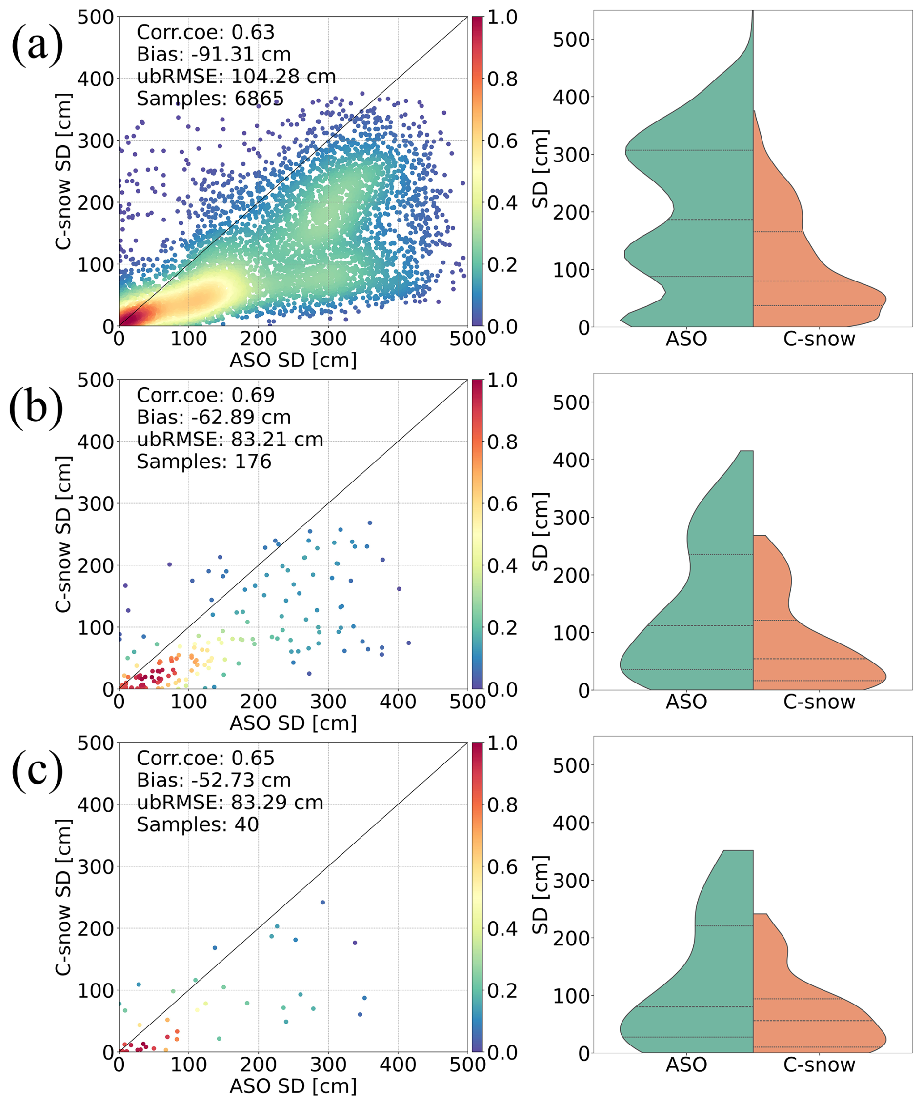
Figure 6 Comparisons (left column) and distributions (right column) between C-snow SD products and ASO SD at different scales, where panels (a), (b), and (c) represent scales of 1, 10, and 25 km, respectively. The dashed lines in the right column indicate the 25th, 50th, and 75th percentiles.

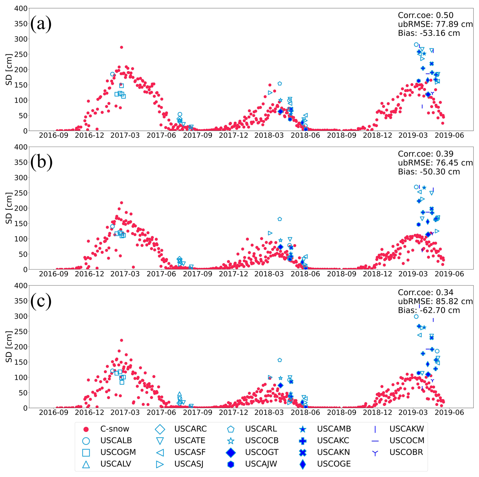
Figure 7 Time series comparison of C-snow products with ASO observations averaged across multiple basins in California and Colorado at (a) 1 km, (b) 10 km, and (c) 25 km scales. The red points represent the average daily C-snow SD in all the selected basins, and the different blue symbols indicate the daily average ASO data in various basins.

Figure 7 shows a comparison of time series of the C-snow SDs and ASO observations in different basins at three scales. At all scales, the C-snow retrievals match well with the ASO data in 2017. In 2018, when the ASO observations were primarily concentrated between March and June, the C-snow retrieval results were underestimated because of wet snow. During the heavy snow season of 2019, compared with the ASO data, the C-snow SD data significantly underestimated the SD and fail to accurately capture the changes in snowpack during this period.

3.2 Different scale patterns of C-snow retrievals with station and ASO measurements

We compared the C-snow retrievals with both station data and ASO observations across various scales, with different trends identified with increasing scale. Compared with that of the station data, the accuracy of the C-snow data tended to decrease as the scale increased, whereas the accuracy of the ASO data tended to increase (Fig. 8a). Furthermore, we compared the station data and ASO observations (Fig. 8b). There is a significant correlation between the station and ASO data, with a corr.coe of 0.92. Moreover, the bias is −12.19 cm, and the ubRMSE is 22.91 cm, indicating that some errors remain. Thus, the uncertainty of the ASO data may affect the results, although the data are reliable.

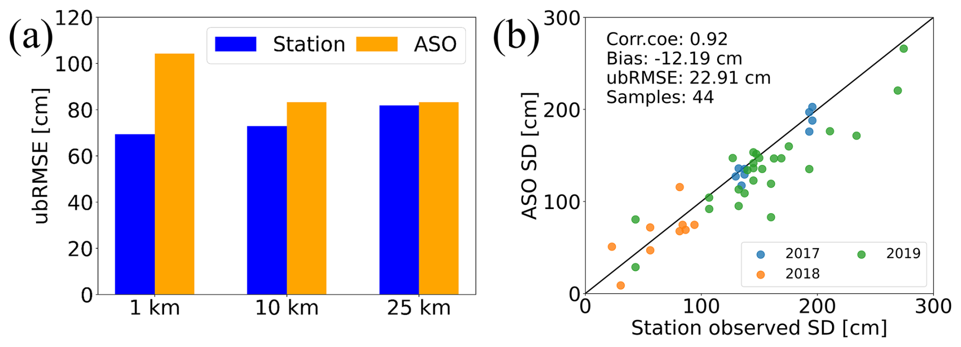
Figure 8 (a) Accuracy performance of the C-snow product at different scales when station observations and ASO SD data are used as reference data and (b) a comparison of station data and ASO observations (3 m ASO data are used to match the station data).

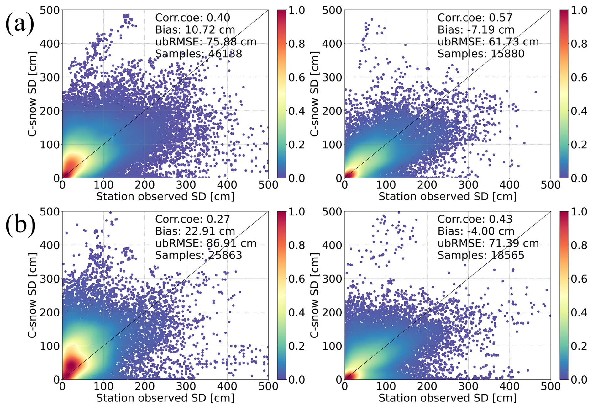
Figure 9 Impact of the number of stations within grids at the (a) 10 km and (b) 25 km scales on the accuracy of the C-snow product. The left column presents the C-snow evaluation result when there is only one station within the grid, and the right column presents the evaluation result when there is more than one station within the grid.

To investigate the contrasting accuracy trend, we counted the number of stations within each grid at the 10 and 25 km scales (Fig. A2). We found that most grids, namely, 63.06 % at the 10 km scale and 51.09 % at the 25 km scale, contain only one station. We compared the accuracy of the C-snow retrievals from grids with only one station and those with more than one station (Fig. 9). The results show that the performance of C-snow is related to the number of stations in the sample grids. For example, at the 10 km scale, corr.coe increases from 0.40 to 0.57, and ubRMSE decreases from 75.88 to 61.73 cm with increasing number of stations. At the 25 km scale, the improvement in accuracy is also obvious, with the corr.coe improving from 0.27 to 0.43 and the ubRMSE decreasing from 86.91 to 71.39 cm. In addition, the C-snow retrievals from grids with only one station are overestimated, and the bias ranges from 10.72 to 22.91 cm. For grids with more than one station, the C-snow retrievals are typically underestimated, with biases ranging from −4.00 to −7.19 cm.

3.3 Effects of landscape and terrain on the SD retrieval results

The impact of land cover on C-snow accuracy was investigated at different scales, as shown in Fig. 10. Here, station measurements were used as reference data because of their global coverage. In forested regions, C-snow tends to be slightly underestimated in general. The accuracy decreases with increasing scale, with corr.coe decreasing from 0.53 to 0.37 and ubRMSE increasing from 67.90 to 72.57 cm. In the permanent ice region, the C-snow product includes several abnormally overestimated results, especially at the 10 and 25 km scales, with a bias greater than 290 cm. For the other types, C-snow also displays a decrease in accuracy at 10 and 25 km resolutions compared with that at the 1 km scale.

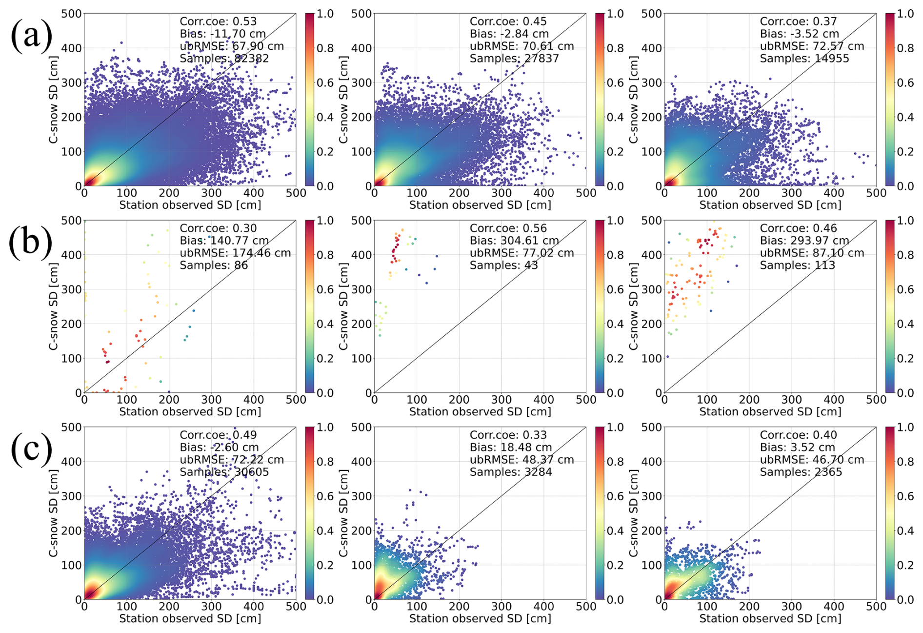
Figure 10 Impact of various land cover types on the accuracy of C-snow products at different scales: (a) tree cover, (b) permanent ice, and (c) other types. The left column represents the scale of 1 km, the middle column represents the scale of 10 km, and the right column represents the scale of 25 km.

The presence of permanent ice results in large errors in the accuracy of C-snow at different scales (Fig. 10). We analyzed the errors in the C-snow product as the coverage of permanent ice within the grids increased at the 10 and 25 km scales (Fig. 11). With increasing permanent ice coverage, the bias gradually increases at both the 10 and 25 km scales, clearly indicating an overestimation trend (Fig. 11a). Moreover, the ubRMSE also tends to increase from 70.08 to 232.51 cm, indicating high uncertainty due to the presence of permanent ice (Fig. 11b).

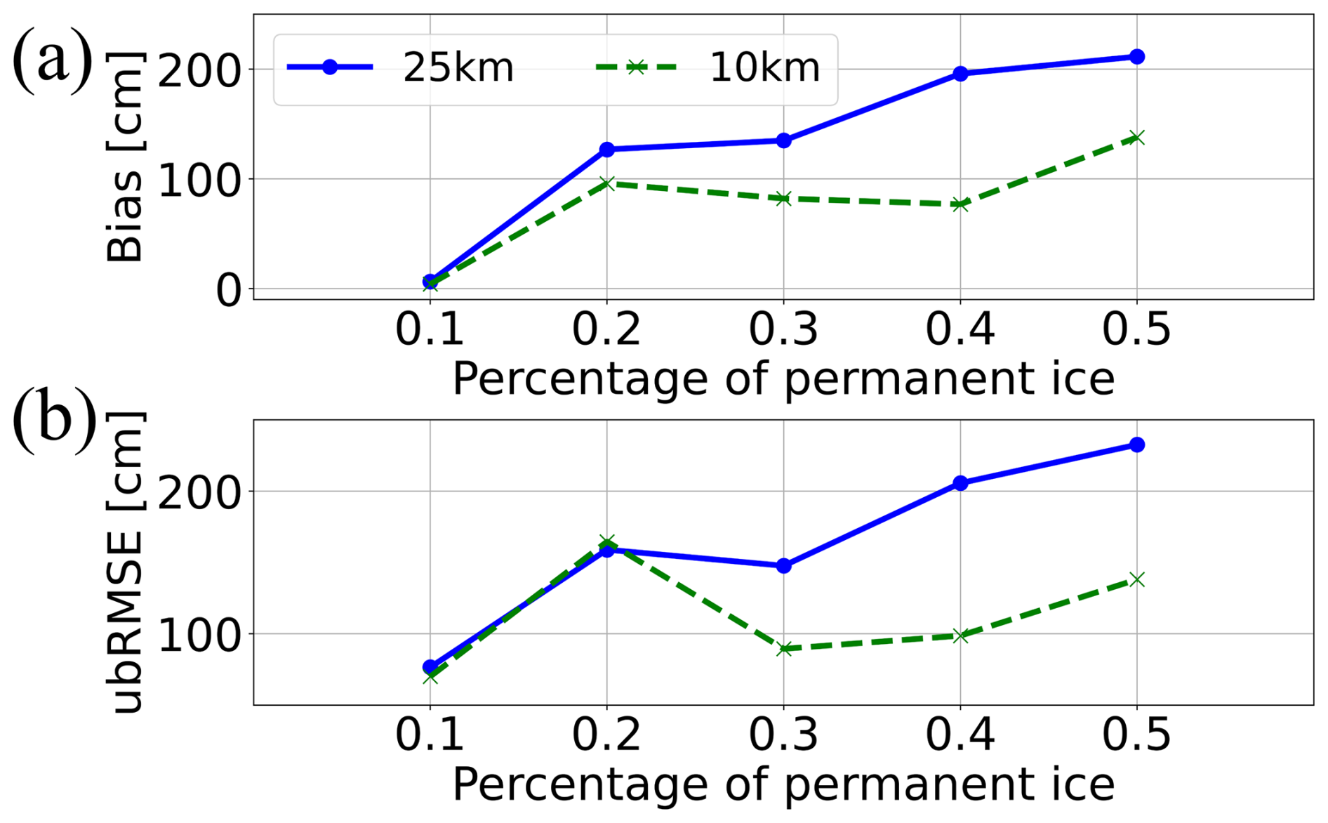
Figure 11 Effects of permanent ice on the accuracy of the C-snow product at different scales, including (a) bias and (b) ubRMSE, which are statistics based on the station dataset.

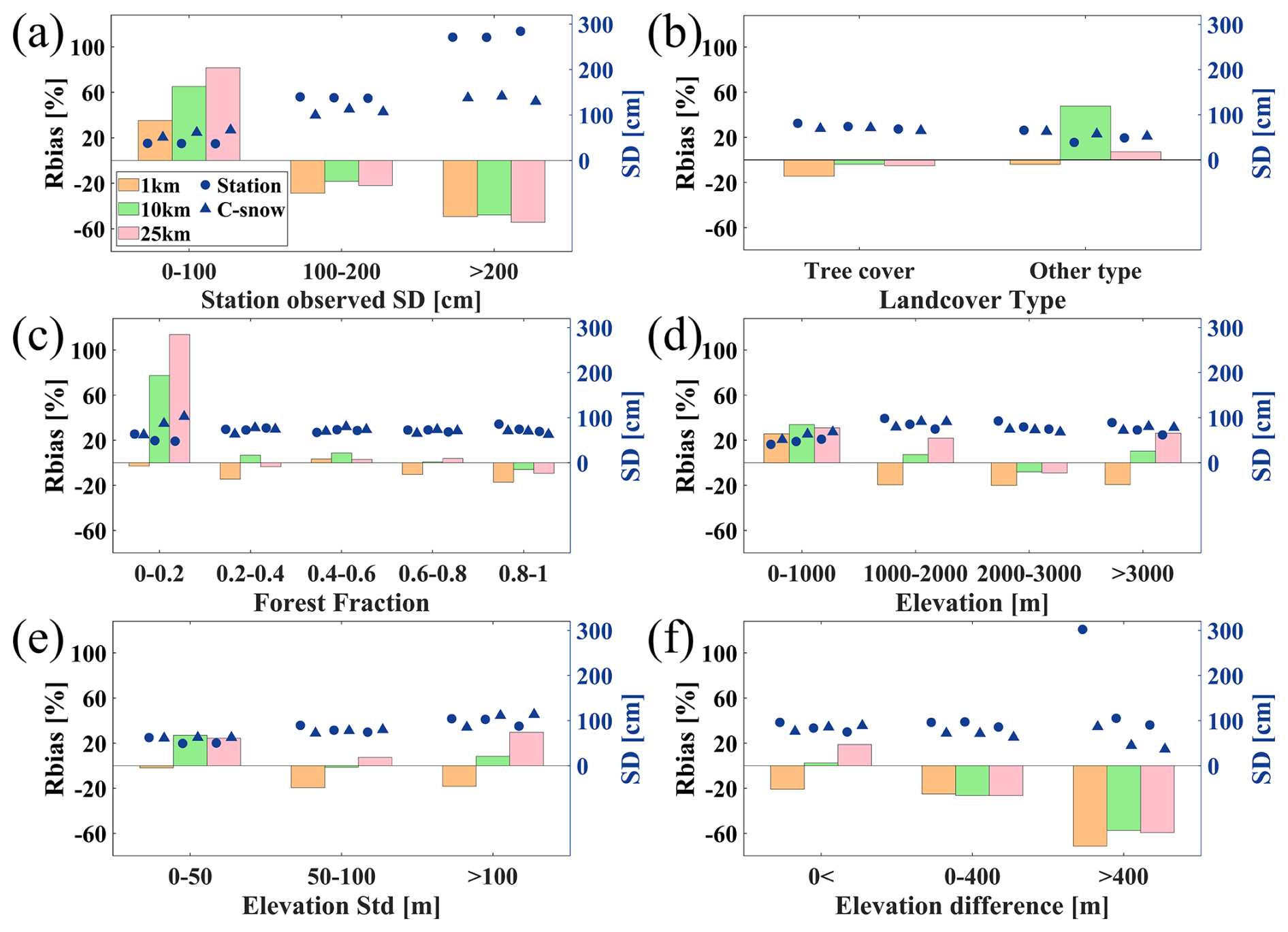
Figure 12 Impact of different (a) station-observed SD, (b) land cover types, (c) forest fractions, (d) elevations, (e) standard deviations of elevation, and (f) elevation differences between stations and grids on the accuracy of C-snow SD products across various scales. The bars indicate the Rbias between the C-snow and station-observed snow SD, while the markers show the average SD from the stations and the C-snow product. The left axis corresponds to Rbias, and the right axis corresponds to the average SD.

Figure 12 shows the impact of the SD conditions and various geographic environments on the accuracy of the C-snow data at different scales. Here, the samples with permanent ice cover were excluded from the validation data because of large errors (see Fig. 10b). When the SD at a station is less than 100 cm, all three scales are overestimated (Fig. 12a). The overestimation becomes more pronounced as the scale increases, with Rbias increasing from 35.16 % at 1 km to 81.68 % at 25 km. In contrast, when the SD exceeds 100 cm, it is underestimated at all scales. The underestimation is relatively small at the 10 km scale, where Rbias reaches −47.79 % when the SD is greater than 200 cm. With respect to tree cover, the results at the three scales tend to be underestimated (Fig. 12b). For the other land cover types, Rbias at the 10 km scale reaches as high as 47.64 %, indicating significant overestimation. When the forest fraction is between 0 and 0.2, significant overestimation occurs at both the 10 and 25 km scales, with Rbias values of 77.33 % and 113.74 %, respectively (Fig. 12c).

At elevations below 1000 m, the C-snow product is overestimated at the 1 km scale, with an Rbias of 25.75 %, whereas it is underestimated at all other elevation intervals (Fig. 12d). For elevations between 2000 and 3000 m, the values at both the 10 and 25 km scales are underestimated, with Rbias values of −8.14 % and −8.95 %, respectively. When the standard deviation of elevation is between 50 and 100 m, C-snow is underestimated at the 1 km scale, with an Rbias value of −19.41 % (Fig. 12e). When the standard deviation of the elevation is greater than 100 m, the C-snow values at both the 10 and 25 km scales are overestimated, with Rbias values reaching 29.60 %. We also find that C-snow performs best in areas with moderate standard deviations of elevation (50–100) and moderately to highly forested (0.4–0.8) areas. As the difference in elevation between the station and the grid increases, an underestimation trend is observed at all scales, with Rbias ranging from 18.83 % to −59.35 % at the 25 km scale (Fig. 12f). When the station elevation is lower than the grid elevation (elevation difference < 0), underestimation is observed only at the 1 km scale, with an Rbias of −22.88 %.

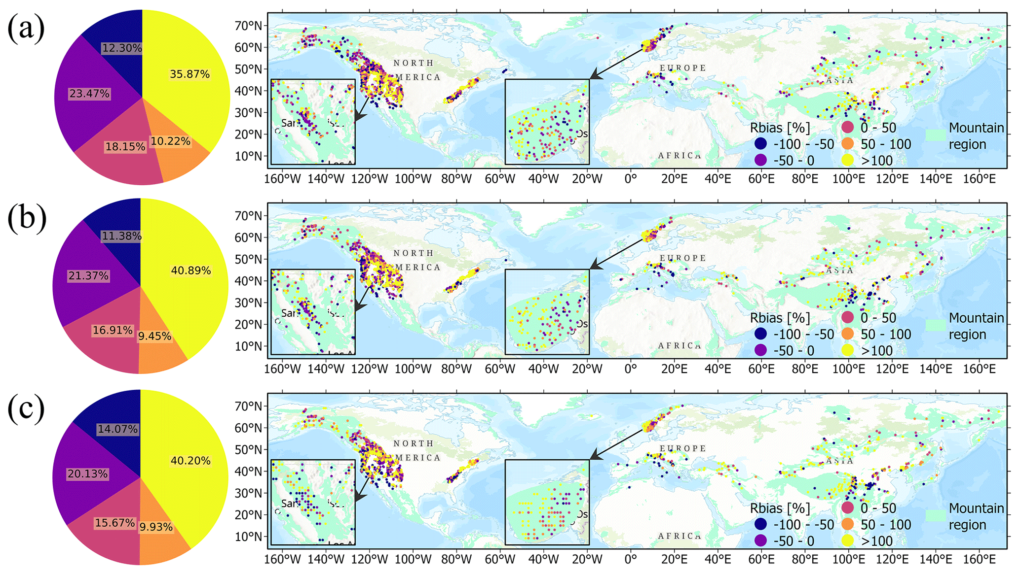
Figure 13 Pie charts (left column) and spatial distributions (right column) of Rbias at (a) 1 km, (b) 10 km, and (c) 25 km scales. Basemap sources: Esri, TomTom, Garmin, FAO, NOAA, USGS, EPA, USFWS.

Figure 13 shows the spatial distributions of Rbias at different scales. A total of 35.77 % of the grids with Rbias values lower than 0 are underestimated at the 1 km scale, and 35.87 % of the grids with Rbias values greater than 100 % are significantly overestimated, especially in the western mountain ranges of the US, the Appalachian Mountains, the southern part of the Scandinavian Mountains, the European Alps, and the Hindu–Kush Himalayas. Moreover, this trend becomes more pronounced with increasing scale, with Rbias values greater than 100 % accounting for 40.89 % and 40.20 % of all the values at the 10 and 25 km scales, respectively.

To explore the influence of complex geography on C-snow retrieval, we selected three nested grids of C-snow retrieval results at different scales (1, 10, and 25 km) and the corresponding station observation data. Figure 14 displays the discrepancies in geographic environments among these nested grids. Within the first and third nested grids, there is only one station, which corresponds to the three-scale grids. In the second nested grid, there are four stations, which correspond to the four 1 km C-snow grids and three 10 km C-snow grids. The average values are calculated for the C-snow product and the station observations.

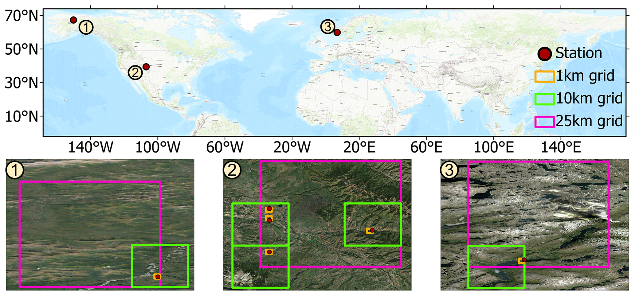
Figure 14 Spatial locations of the three selected nested grids, with the first at 67.45° N, −150.31° E; the second at 39.42° N, −107.00° E; and the third at 56.00° N, 6.85° E. Basemap sources: Esri, TomTom, Garmin, FAO, NOAA, USGS, Microsoft, Vantor.

In the first nested grid, the station observations generally match the C-snow retrieval results at three scales (Fig. 15a). In the second nested grid, the station-observed snow cover is quite shallow, whereas the C-snow values at three scales are overestimated relative to the station observations, especially during the period from December 2016 to March 2017 (Fig. 15b). In the third nested grid, the time series changes at the 1 km scale for C-snow closely match those of the station observations, whereas the C-snow retrieval results are overestimated relative to the station observations at both the 10 and 25 km scales (Fig. 15c). Moreover, we find a large discrepancy between the C-snow at the 10 and 25 km scales.

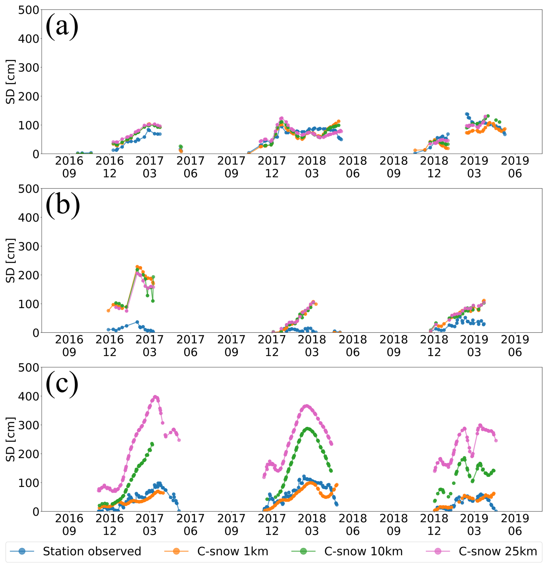
Figure 15 Time series of the SD at different scales (1, 10, and 25 km) for three selected nested grids, where panels (a), (b), and (c) represent the results for the first, second, and third grids, respectively.

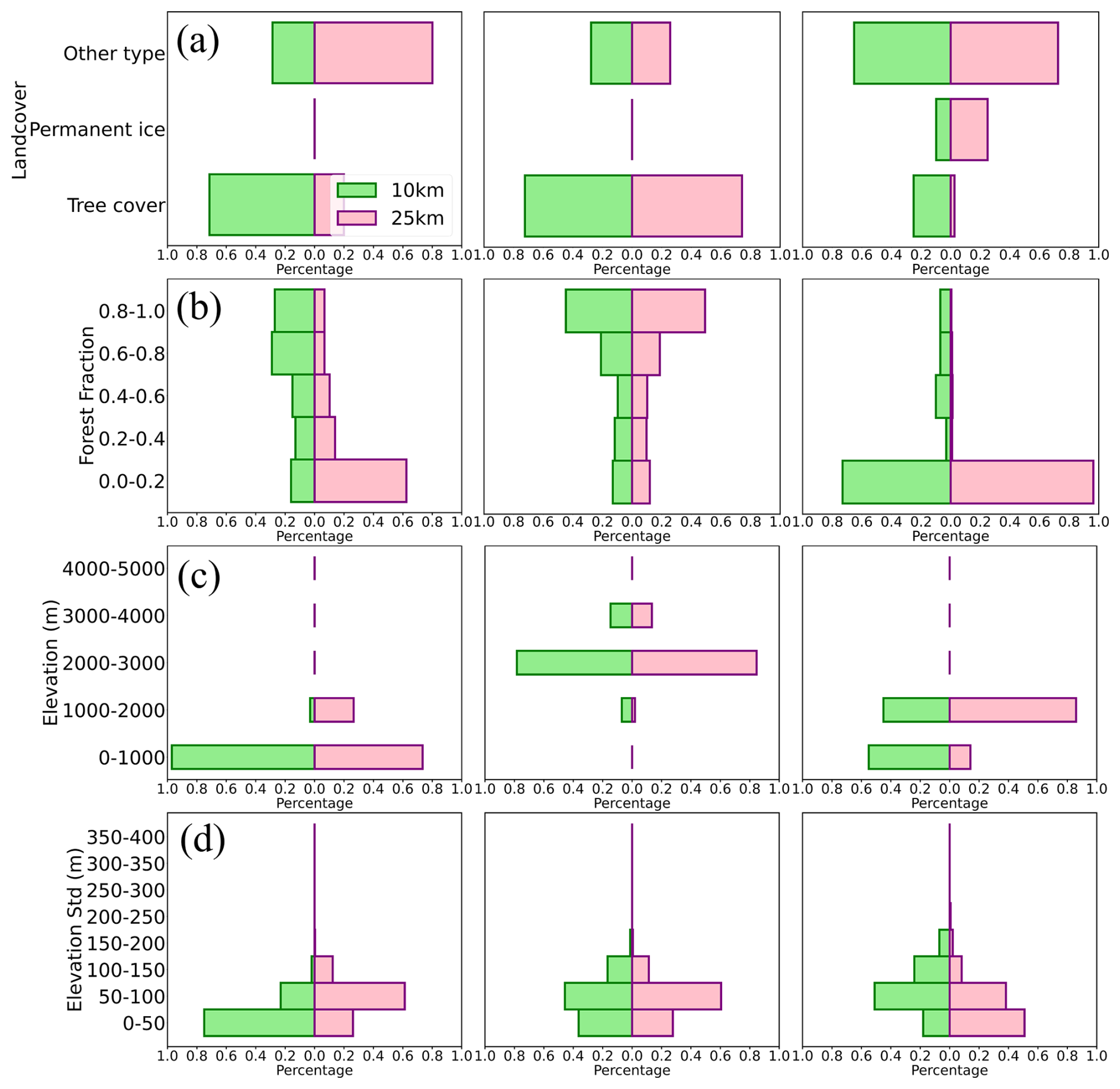
Figure 16 Distributions of (a) land cover types, (b) forest fraction, (c) elevation, and (d) standard deviation of elevation in three selected nested grids, with the left, middle, and right columns representing the first, middle, and third grids, respectively.

To explain the scale effects associated with geographical heterogeneity, we calculated the differences between the 10 and 25 km grids in terms of land cover type, forest fraction, elevation, and standard deviation of elevation (Fig. 16). For the first nested grid, the terrain is predominantly low-elevation (below 1000 m) at both the 10 and 25 km scales, which shows lower spatial variability than high-elevation regions do. Moreover, when the snowpack is less than 100 cm, the C-snow retrievals perform well (Figs. 4 and 5). Thus, the C-snow retrievals at 1, 10 and 25 km are in good agreement with the station observations. For the second nested grid, the geographic environments at the 10 and 25 km scales are very similar; thus, the SD retrievals at both scales are similar. However, the terrain is very complex, e.g., high elevation (2000–3000 m) and high topographic relief (0–200). Thus, the representativeness of the stations may be problematic, resulting in poor agreement with the C-snow retrieval results. For the third nested grid, we find that the heterogeneity of the 10 and 25 km grids is high. For example, the coverage of permanent ice (24.96 %) at the 25 km scale is high relative to that at the 10 km scale, whereas the tree cover fraction (25 %) in the 10 km grid is high. Additionally, the terrain is more complex in the 25 km grid than in the 10 km grid, e.g., at high altitudes. The overestimation occurs mainly because of permanent ice, which is consistent with the results in Fig. 10. The large differences (scale effects) in the SD retrieval results at the 10 and 25 km scales are related to the heterogeneity of the geographic environment. Specifically, the greater the heterogeneity of the geographic environment between the 10 and 25 km scales is, the greater the differences in the SD retrievals.

4 Discussion

The differences in C-snow validation results across scales arise from multiple interacting factors, including the type of validation dataset (point-scale station data vs. spatially dense ASO data), the representativeness of observations within each grid, terrain complexity, land cover composition, spatial aggregation effects, and other environmental influences. Our findings are consistent with previous research on C-snow product evaluation. For instance, Alfieri et al. (2022) reported RMSE values ranging from 20 to 60 cm in the Po River Basin, which aligns with our results at finer scales (e.g., 1 km). Sourp et al. (2025) reported RMSE values between 21 and 138 cm in the Sierra Nevada region, with biases reaching −124 cm, which corroborates our ASO-based validation results. Importantly, our analysis further demonstrates that these errors exhibit different scale-dependent trends.

Compared with that of the station data, the accuracy of the C-snow data tends to decrease as the scale increases, whereas the accuracy of the ASO data tends to increase. This discrepancy can be attributed to the inherent differences in the nature of these validation datasets (Fig. 8). Station measurements are point-scale observations, which makes it difficult to reflect the distribution of SD over large areas. In contrast, ASO provides dense sampling data, which can better represent the spatial distribution of SD. This allows ASO data to more accurately reflect the overall snow conditions within a given area, thereby improving the validation accuracy as the scale increases. Although ASO data have better spatial continuity, their coverage is relatively limited. The accuracy of LiDAR-derived SD is also affected by factors such as terrain and vegetation cover (Enderlin et al., 2022; Neuenschwander et al., 2020; Klápště et al., 2020). Within the coverage scope of the ASO data, steep slopes (as high as 80°) and high forest fractions (mean value of 53 %) likely affect the accuracy of the observations (Fig. A1).

When station data are used for the validation of satellite products, reasonably converting to spatial scales is a key issue. The method used to convert point-scale observations to the spatial scale of satellite pixels also affects the validation results (Fassnacht and Deems, 2006; Hou et al., 2022). Beforehand, we tested and compared the mean and median sampling methods and observed similar validation outcomes. Therefore, this study employs a simple averaging approach, despite its partial neglect of spatial variability (Ge et al., 2019). Although simple averaging methods are easy to use, they cannot fully consider the impact of complex factors such as topography and vegetation distribution on the spatial distribution of the SD, which may lead to deviations in the validation results. In addition, the number of stations affects the validation results. Most grids at the 10 and 25 km scales contain only one station. On one hand, a single station observation may not adequately represent the snow depth across the entire grid. Our test demonstrated that the accuracy of the C-snow product improves when multiple stations are present within a grid cell (Fig. 9). On the other hand, due to the sparsity of station observations, spatial aggregation results are hardly influenced by the choice of interpolation method. Therefore, it is fundamentally necessary to collect more observational data to enhance spatial representativeness, e.g., satellite-based lidar and altimeter estimates. Then future research can use more advanced spatial interpolation methods, such as interpolation methods based on geographically weighted regression or machine learning algorithms, to more accurately reflect the spatial changes in the SD and thus improve the validation.

The presence of permanent ice significantly affects the accuracy of the C-snow product. As the coverage of permanent ice within the grids increases, the bias and ubRMSE also increase, indicating an overestimation trend (Fig. 11). Permanent ice exhibits electromagnetic properties similar to those of snowpacks, increasing the backscattering of radar signals (Scott et al., 2006). During the melt season, an increase in the roughness of the ice surface leads to an increase in the backscattering coefficient (Baumgartner et al., 1999). The dynamic nature of glaciers, characterized by crevasses and glacier movement, can lead to temporal variations in the backscattering coefficient (Sander and Bickel, 2007; Brock, 2010), complicating interactions between radar signals and snow characterization. Thus, quality control of spatially sampled C-snow products, especially at coarse scales, must be performed to ensure that the retrieval results in permanent ice-covered areas are filtered and removed. These limitations may cause deviations or uncertainties in the retrieval results of the C-snow product in these specific areas. To overcome these limitations, future research can explore improved retrieval algorithms to better separate snow signals from glacial backgrounds and conduct multisource data fusion retrieval using other remote sensing data sources, thereby enhancing the applicability of the C-snow product in complex environments. Moreover, combining field observations and model simulations to study in depth the interaction mechanism between snow physical processes and radar signals can provide theoretical support for improving the C-snow product.

5 Conclusion

In this study, we evaluated and compared the accuracies of the C-snow retrieval results at three spatial scales (1, 10, and 25 km) through station measurements and ASO observations. We also analyzed the factors influencing the accuracy at these scales and explored the inconsistency in scale effects via station and airborne reference datasets. Our results indicate that as the spatial scale increases, the correlation between the C-snow products and station observations significantly decreases, with a corr.coe of 0.52 at the 1 km scale, which decreases to 0.44 at the 10 km scale and 0.32 at the 25 km scale. The error increases with scale, from 69.43 cm at the 1 km scale to 81.87 cm at the 25 km scale. Compared with the airborne ASO data, the C-snow product became increasingly more accurate as the spatial scale increased, with bias values decreasing from −91.31 to −52.73 cm and ubRMSE decreasing from 104.3 to 83.29 cm. These different scale patterns occur mainly because of the different representativeness of station and ASO data.

We also determined that the land cover type affects the accuracy of C-snow classification. In areas covered with tree cover, the accuracy of C-snow significantly decreases as the spatial scale increases, with the corr.coe decreasing from 0.53 to 0.37 and the ubRMSE increasing from 67.90 to 72.57 cm. In areas covered by permanent ice, C-snow consistently overestimates the SD at all scales, which is related to the percentage of ice coverage. The impact of terrain on the accuracy of C-snow is complex. The overestimation of C-snow at the 1 km scale is evident for elevations below 1000 m, whereas the SD tends to be underestimated in other elevation ranges. For elevations between 2000 and 3000 m, the C-snow retrievals at both the 10 and 25 km scales displayed an underestimation trend, with Rbias values of −8.14 % and −8.95 %, respectively. The standard deviation of the elevation also affects the accuracy of C-snow. When the standard deviation of elevation is between 50 and 100 m, C-snow at the 1 km scale is underestimated (Rbias of −19.41 %), and when the standard deviation of elevation is greater than 100 m, C-snow at the 25 km scale is overestimated (Rbias of 29.60 %).

In this study, we assessed the performance of C-snow products at different spatial scales and analyzed the corresponding influencing factors. According to our study, the C-snow products at the three scales are characterized by high uncertainty. In particular, we should be careful when coarse-scale C-snow products are used as a reference, and at a minimum, some outlier data should be filtered and removed. Future research should continue to explore the possibility of improving C-snow retrieval by combining SAR backscattering, polarimetric, interferometric and satellite LiDAR data to increase the reliability and accuracy of Sentinel-1-based products in practical applications.

Appendix A

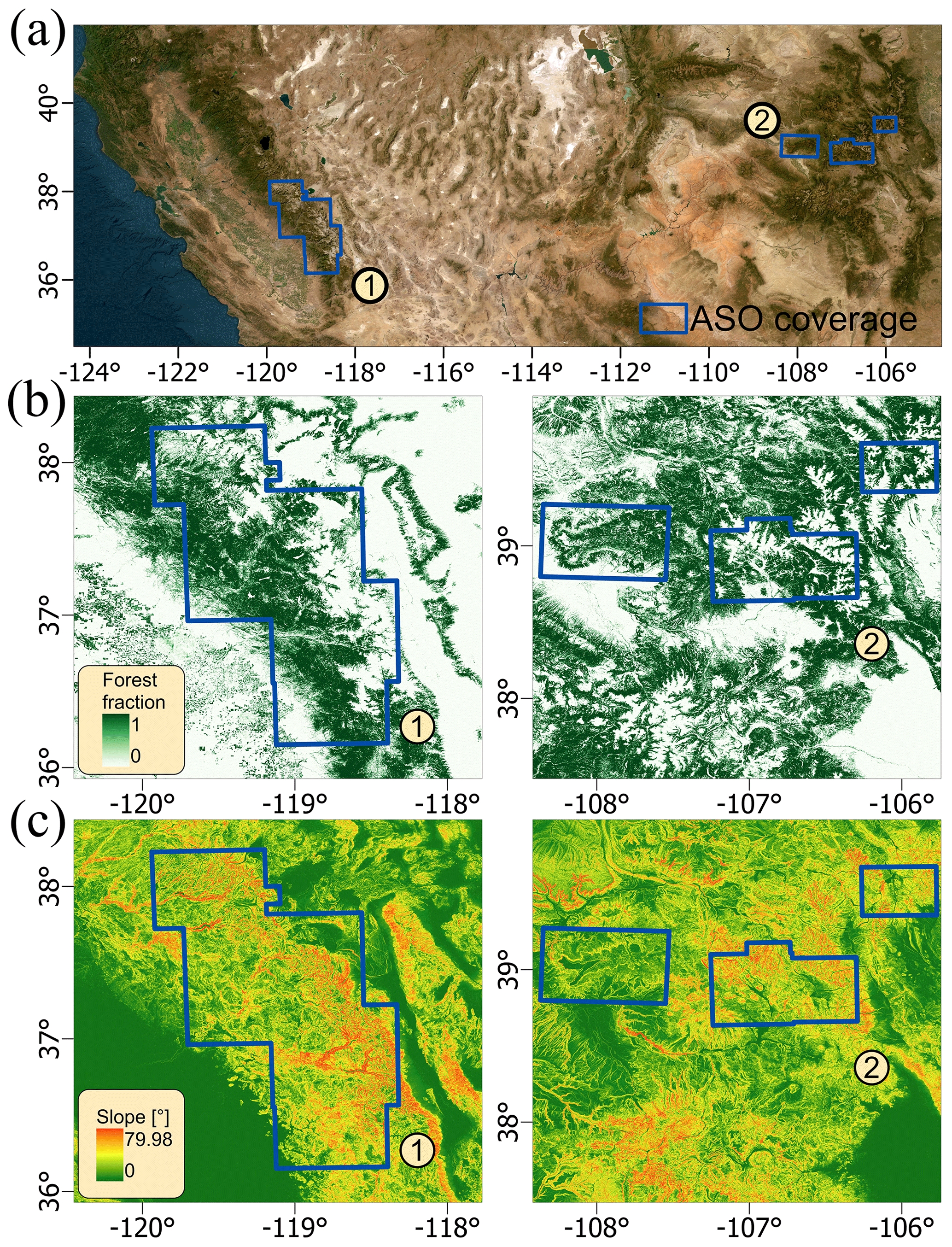
Figure A1 (a) Overall geographical conditions within the coverage area of ASO, with zoomed-in views of (b) the forest fraction and (c) slope conditions. Basemap source: Earthstar Geographics.

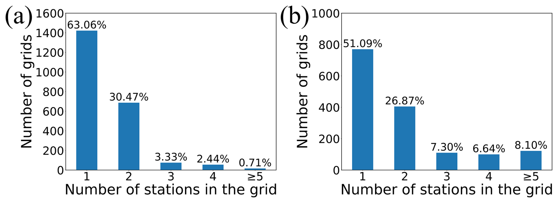
Figure A2 Statistics regarding the number of stations within the grids at scales of (a) 10 km and (b) 25 km.