Modelling L-band microwave brightness temperature time series for firn aquifers

Firn aquifers are important in polar ice sheet hydrology and the associated mass and energy transport processes. Although the firn aquifer extent has been mapped using passive microwave satellite observations, models for predicting the L-band brightness temperature time series have remained elusive. This paper implements a radiative transfer model for time series L-Band V and H-pol brightness temperature (TB) observations from the 3 km SMAP enhanced resolution data product. The model relates the firn aquifer permittivity and properties of the dry firn layer above the aquifer to SMAP observations. Results are presented for aquifers within both the Greenland and Antarctic ice sheets. The results show that the brightness temperature is more sensitive to aquifer liquid water content changes when the water table is closer to the surface. The method provides a tool for the radiometry study of firn aquifer and a theoretical basis for potentially retrieving firn aquifer liquid water content using passive microwave data.

1 Introduction

Summer surface melt in the percolation facets of the Greenland Ice Sheet (GrIs) and the Antarctic Ice Sheet(AIS) is an important process (Mankoff et al., 2021; Lenaerts et al., 2019). An extreme event in 2012, for example, produced surface melt over the entire GrIS (Nghiem et al., 2012). Meltwater is typically expected to refreeze locally within the firn or run off into the ocean. However, under certain conditions, an ice-water mixed layer called the Perennial firn aquifer can remain unfrozen during the winter season. A major discovery of an aquifer occurred in 2011 on the southeastern coast of Greenland during the Arctic Circle Traverse expedition, which involved a drilled borehole and GPR survey (Forster et al., 2014). If drained, the Greenland aquifer could contribute up to a 0.4 mm increase in sea level (Koenig et al., 2014).

Instead of simply acting as a meltwater store, the embedded water can flow and drain the aquifer quickly (Miller et al., 2018), and studies have shown an average aquifer age of 6.5 years (Miller et al., 2020b). This indicates that the aquifer is not buffering the mass loss or the rise of the sea level but perhaps amplifying its contribution. Understanding the aquifer's water content can help close the mass balance of Greenland (Slater et al., 2021; Bamber et al., 2018; Shepherd et al., 2012) and the meltwater routing mechanism.

The mapping of firn aquifers has been studied using airborne GPR data from Operation Ice Bridge (Miège et al., 2016; Chu et al., 2018). The total amount of water was estimated in regions where the ice-ground reflection could be observed, from which the decay due to the aquifer layer could be estimated (Chu et al., 2018). Such studies are limited to the available flight paths, and GPR data were gathered only once yearly in the late spring. Mapping for the horizontal extent of the firn aquifer from satellite data was first performed using Sentinel-1 C-band SAR data (Brangers et al., 2020).

L-band brightness temperatures from the Soil Moisture Active and Passive (SMAP) (Entekhabi et al., 2010; Long et al., 2019) mission satellite have also been used in firn aquifer studies. Brightness temperature data show a sigmoid function shape decrease in brightness temperature from late summer to late spring of the next year due to increased scattering from dry firn (Miller et al., 2020a). The horizontal extent of the Greenland aquifers was then mapped based on time series signatures in enhanced resolution SMAP brightness temperature data. A saturation factor was also derived from time series data to first map the percolation zone and then identify the aquifer and subsurface ice slab (Miller et al., 2022). However, the liquid water content inside the aquifer has not been quantitatively studied. Due to the low absorption of ice and air, thermal emission from a firn aquifer is modulated by the aquifer-firn interface and the dry firn structure above. Though modelling efforts have been made to explain the time series of the brightness temperature, a simple layered random medium model cannot explain the polarization dependence in the measurements (Bringer et al., 2017). The modelled results showed agreement with SMAP H-pol measurements, but the V-pol is 40 K higher than the measurements. This is because the layering structures are not able to account for the depolarization effects due to the assumption of flat interfaces between layers. Such a large difference in the V and H channels would make the parameters used to explain the data much different from each other, hence introducing uncertainties in retrieving properties of the firn aquifer.

Noticing the limitations of the current models, this paper aims to provide a radiative transfer model that can explain the V and H-pol brightness temperature with the same set of parameters. Unlike previous approaches, which cannot match the observed V- and H-polarized brightness temperatures concurrently, the proposed model achieves polarization-consistent simulations, thereby eliminating a major source of uncertainty in future retrieval works. In this model, Three-Dimensional random media is used to describe the random fluctuations of the dry firn density (Tsang et al., 2004; Xu et al., 2023), and the phase matrix used in the radiative transfer model is developed based on this description. A solution based on this model is provided. Time series simulation is also performed based on the hypothesis of decreasing water table depth starting from the end of summer. Such a hypothesis comes from the observation of the land glacier firn aquifer (Christianson et al., 2015). Simulation of the time series is not to justify or falsify the hypothesis, but to show the ability of the new model and provide a possible explanation for the brightness temperature time series. In modelling aquifer thermal emissions, two components need to be characterized. The first is a permittivity model for the firn aquifer, which is the key parameter that relates the firn-aquifer interface reflection to the water content of the aquifer. We use the results from Huang et al. (2024) for the values, as the aquifer is a complex structure of ice-water mixture. The second is a radiative transfer model that accounts for the reflection of thermal emission due to the firn-aquifer interface and for density variations in the dry firn. In the emission problem, the firn-aquifer interface produces upward emissions and also reflects downward-going emissions from the dry firn above. Multiple scattering also occurs within the dry firn layer due to its inhomogeneity. The approach also allows the possibility of estimating the water content of the aquifer remotely.

The analysis considers 3 km enhanced resolution SMAP brightness temperature time series data for locations in Greenland and Antarctica. For Greenland, the 3 km pixel covering FA-13 (66.1812, −39.0435) (Koenig et al., 2014) is studied. FA-13 provides in situ measurements of density (Sumup data set, Montgomery et al., 2018), temperature (Miège et al., 2020b), and water level depth (position of aquifer upper boundary). The location lies on a 2014 survey path of the University of Kansas Accumulation Radar (CReSIS, 2024). The other location lies on the Wilkins Ice Shelf (Montgomery et al., 2020) , Antarctica, where a field investigation was performed in Dec 2018. The investigation provides information on the density profile and the water table depth. Temperature and liquid water content information are not available in this location; other in situ information on the Wilkins Ice Shelf is available on the website of the U.S. Antarctic Program (USAP) Data Center (Miège et al., 2020a). Information from the in-situ measurements is applied with the forward model to simulate SMAP V and H-pol brightness temperatures. Data collected from winter 2015 to summer 2016 in Greenland and during 2018 for the Wilkins Ice Shelf is analysed.

The next section illustrates the physical model for the thermal emission problem. First, mathematical derivations for the radiative transfer model are described, and a discussion of aquifer permittivity is then provided. Data sets used are discussed. In Sect. 3, the numerical results are presented together with the SMAP measurements over Greenland's east coast from winter 2015 to Spring 2016 and over Wilkins Ice Shelf in 2018. Additional discussions and conclusions are then provided in Sects. 4 and 5, respectively.

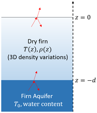
Figure 1 A two-layer model for the firn aquifer emission problem in the early spring before the surface melt starts. The top region is air (z>0), the middle region is dry firn with changing properties. The density fluctuation in this region is considered as 3 dimensional. The lower part is a firn aquifer with a constant temperature of T₀=273.15.

2 Method

The model describes a firn aquifer as the two-region structure illustrated in Fig. 1: dry firn on top of a saturated aquifer. The thickness of the dry firn layer is denoted as d, where $z=-d$ is the water level depth (upper aquifer boundary). The dry firn is described as a random medium having permittivity fluctuations (due to ice density variations) in both the vertical and horizontal directions, as well as a mean value that varies with depth. The mean density profile is obtained by fitting the borehole density measurements with an exponential curve. The fluctuating profile is characterized by the following correlation function:

$$\begin{array}{}\text{(1)}& C\left(\mathit{r},\mathit{r}{}^{\prime }\right)={\mathrm{\Delta }}^{\mathrm{2}}\exp \left(-{\displaystyle \frac{\left|z-z{}^{\prime }\right|}{l_z}}\right)\exp \left(-{\displaystyle \frac{{\left|{\mathit{r}}_{\perp }-{\mathit{r}}_{\perp }{}^{\prime }\right|}^{\mathrm{2}}}{l_{\mathit{\rho }}^{\mathrm{2}}}}\right)\end{array}$$

where Δ=SD(ρ) is the standard deviation of the density fluctuations, with l_z and l_ρ the vertical and horizontal correlation lengths. Density fluctuations in the vertical direction are modelled as exponentially correlated, while those in the horizontal direction are modelled with a Gaussian function. The exponential correlation function captures the high-frequency changes, while the Gaussian reflects more low-frequency changes in the structure. This model of 3D variations was previously used to model brightness temperatures over the accumulation zone in Greenland (Xu, 2024); the 3-dimensional variations represented cause angular and polarization coupling between V and H polarizations that was found to improve the match to measured data. Previously, the lower boundary of the variation region was considered to have no reflection. In this case, due to the existence of a firn aquifer, the reflection from this boundary could not be ignored. Because aquifers usually exist in the percolation zone of the ice sheet, their density properties can be very different from those in the accumulation zone, where the freeze-thaw process is rare. Borehole measurements indicate a high-density variation profile in the firn above an aquifer.

2.1 Radiative transfer model in the dry zone region

The emission can be described in the dry zone region by the coupled radiative transfer equations; the geometry of the model is presented in Fig. 1:

$$\begin{array}{}\text{(2)}& {\displaystyle }\begin{array}{rl}\cos \mathit{\theta }{\displaystyle \frac{d}{\mathrm{d}z}}{\mathit{T}}_{\mathrm{u}}\left(\mathit{\theta },z\right)& =-{\overleftrightarrow{\mathit{\kappa }}}_{\mathrm{e}}\left(\mathit{\theta },z\right){\mathit{T}}_{\mathrm{u}}\left(\mathit{\theta },z\right)+{\mathit{\kappa }}_{\mathrm{a}}\left(z\right)T_{\mathrm{0}}\left(z\right)\\ & +\underset{\mathrm{0}}{\overset{\frac{\mathit{\pi }}{\mathrm{2}}}{\int }}\mathrm{d}\mathit{\theta }{}^{\prime }\sin \mathit{\theta }{}^{\prime }[\overleftrightarrow{P}\left(\mathit{\theta },\mathit{\theta }{}^{\prime },z\right){\mathit{T}}_{\mathrm{u}}\left(\mathit{\theta }{}^{\prime },z\right)\\ & +\overleftrightarrow{P}\left(\mathit{\theta },\mathit{\pi }-\mathit{\theta }{}^{\prime },z\right){\mathit{T}}_{\mathrm{d}}(\mathit{\theta }{}^{\prime },z)]\end{array}\text{(3)}& {\displaystyle }\begin{array}{rl}-\cos \mathit{\theta }{\displaystyle \frac{d}{\mathrm{d}z}}{\mathit{T}}_{\mathrm{d}}\left(\mathit{\theta },z\right)& =-\overleftrightarrow{{\mathit{\kappa }}_{\mathrm{e}}}\left(\mathit{\theta },z\right){\mathit{T}}_{\mathrm{d}}\left(\mathit{\theta },z\right)+{\mathit{\kappa }}_{\mathrm{a}}\left(z\right)T_{\mathrm{0}}\left(z\right)\\ & +\underset{\mathrm{0}}{\overset{\frac{\mathit{\pi }}{\mathrm{2}}}{\int }}\mathrm{d}\mathit{\theta }{}^{\prime }\sin \mathit{\theta }[\overleftrightarrow{P}\left(\mathit{\pi }-\mathit{\theta },\mathit{\theta }{}^{\prime },z\right){\mathit{T}}_{\mathrm{u}}\left(\mathit{\theta }{}^{\prime },z\right)\\ & +\overleftrightarrow{P}\left(\mathit{\pi }-\mathit{\theta },\mathit{\pi }-\mathit{\theta }{}^{\prime },z\right){\mathit{T}}_{\mathrm{d}}(\mathit{\theta }{}^{\prime },z)]\end{array}\end{array}$$

where T_u(θ,z) and T_d(θ,z) are the upward and downward brightness temperatures, $\overleftrightarrow{{\mathit{\kappa }}_{\mathrm{e}}}(\mathit{\theta },z)$ is the extinction coefficient matrix, κ_a(z) is the absorption coefficient. $\overleftrightarrow{P}(\mathit{\theta },\mathit{\theta }{}^{\prime },z)$ is the phase matrix that couples the brightness temperature in θ^′ to the direction of θ. The parameters in the radiative transfer equations are functions of depth. This is because the temperature and density profiles vary according to the depth. The radiative transfer equations are subject to the boundary conditions:

$$\begin{array}{}\text{(4)}& {\displaystyle }{\mathit{T}}_{\mathrm{d}}\left(\mathit{\theta },z=\mathrm{0}\right)=\overleftrightarrow{R_{\mathrm{10}}}\left(\mathit{\theta }\right){\mathit{T}}_{\mathrm{u}}(\mathit{\theta }z=\mathrm{0})\text{(5)}& {\displaystyle }\begin{array}{rl}{\mathit{T}}_{\mathrm{u}}\left(\mathit{\theta },z=-d\right)& =\overleftrightarrow{R_{\mathrm{12}}}\left(\mathit{\theta }\right){\mathit{T}}_{\mathrm{d}}\left(\mathit{\theta },z=-d\right)\\ & +\left(\mathrm{1}-\overleftrightarrow{R_{\mathrm{12}}}\left(\mathit{\theta }\right)\right)T_{\mathrm{aquifer}}\end{array}\end{array}$$

where $\overleftrightarrow{R_{\mathrm{10}}}\left(\mathit{\theta }\right)$ and $\overleftrightarrow{R_{\mathrm{12}}}\left(\mathit{\theta }\right)$ are diagonal reflectivity matrices for the dry firn-air interface (the upper boundary of the dry firn region) and the dry firn-aquifer interface (the lower boundary of the dry firn region). At the dry firn-aquifer interface, the brightness temperature emitted from the aquifer is transmitted into the dry firn region, as indicated by the term. $\left(\mathrm{1}-\overleftrightarrow{R_{\mathrm{12}}}\left(\mathit{\theta }\right)\right)T_{\mathrm{aquifer}}$ where T_aquifer is the aquifer's physical temperature.

The radiative transfer equations are solved using an iterative approach. The differential equations are converted into integral equations that express the upward and downward brightness temperature in terms of integrals. Details on how to obtain the expressions are documented in Xu (2024), and major steps are listed in the Appendix. The integral expression and the 0th solution are provided in the appendix. The nth-order solutions are obtained by substituting the n−1th-order term inside the scattering expressions as:

$$\begin{array}{}\text{(6)}& {\displaystyle }\begin{array}{rl}& {{\mathit{T}}_{\mathbf{u}}}^n\left(\mathit{\theta }z\right)={\mathit{S}}^n\left(\mathit{\theta }z\right)\\ & +{\left[I-{\overleftrightarrow{r}}_{\mathrm{10}}\left(\mathit{\theta }\right){\overleftrightarrow{r}}_{\mathrm{12}}\left(\mathit{\theta }\right)\exp \left(-\mathrm{2}\sec \mathit{\theta }{\int }_{-d}^{\mathrm{0}}\overleftrightarrow{{\mathit{\kappa }}_{\mathrm{e}}}\left(\mathit{\theta },z^{\prime \prime }\right)\mathrm{d}{z}^{\prime \prime }\right)\right]}^{-\mathrm{1}}\\ & {\overleftrightarrow{r}}_{\mathrm{12}}\left(\mathit{\theta }\right){\mathit{W}}^n(\mathit{\theta },-d)\exp \left(-\sec \mathit{\theta }{\int }_{-d}^z\overleftrightarrow{{\mathit{\kappa }}_{\mathrm{e}}}\left(\mathit{\theta },z^{\prime \prime }\right)\mathrm{d}{z}^{\prime \prime }\right)\\ & +{\left[I-{\overleftrightarrow{r}}_{\mathrm{10}}\left(\mathit{\theta }\right){\overleftrightarrow{r}}_{\mathrm{12}}\left(\mathit{\theta }\right)\exp \left(-\mathrm{2}\sec \mathit{\theta }{\int }_{-d}^{\mathrm{0}}\overleftrightarrow{{\mathit{\kappa }}_{\mathrm{e}}}\left(\mathit{\theta },z^{\prime \prime }\right)\mathrm{d}{z}^{\prime \prime }\right)\right]}^{-\mathrm{1}}\\ & {\overleftrightarrow{r}}_{\mathrm{10}}\left(\mathit{\theta }\right){\overleftrightarrow{r}}_{\mathrm{12}}\left(\mathit{\theta }\right)\exp \left(-\sec \mathit{\theta }{\int }_{-d}^z\overleftrightarrow{{\mathit{\kappa }}_{\mathrm{e}}}\left(\mathit{\theta },z^{\prime \prime }\right)\mathrm{d}{z}^{\prime \prime }\right)\\ & \exp \left(-\sec \mathit{\theta }{\int }_{-d}^{\mathrm{0}}\overleftrightarrow{{\mathit{\kappa }}_{\mathrm{e}}}\left(\mathit{\theta },z^{\prime \prime }\right)\mathrm{d}{z}^{\prime \prime }\right){\mathit{S}}^n(\mathit{\theta },\mathrm{0})\end{array}\text{(7)}& {\displaystyle }\begin{array}{rl}& {{\mathit{T}}_{\mathbf{d}}}^n\left(\mathit{\theta }z\right)={\mathit{W}}^n\left(\mathit{\theta }z\right)\\ & +{\left[I-{\overleftrightarrow{r}}_{\mathrm{12}}\left(\mathit{\theta }\right){\overleftrightarrow{r}}_{\mathrm{10}}\left(\mathit{\theta }\right)\exp \left(-\mathrm{2}\sec \mathit{\theta }{\int }_{-d}^{\mathrm{0}}\overleftrightarrow{{\mathit{\kappa }}_{\mathrm{e}}}\left(\mathit{\theta },z^{\prime \prime }\right)\mathrm{d}{z}^{\prime \prime }\right)\right]}^{-\mathrm{1}}\\ & \exp \left(-\sec \mathit{\theta }{\int }_z^{\mathrm{0}}\overleftrightarrow{{\mathit{\kappa }}_{\mathrm{e}}}\left(\mathit{\theta },z^{\prime \prime }\right)\mathrm{d}{z}^{\prime \prime }\right){\overleftrightarrow{r}}_{\mathrm{10}}\left(\mathit{\theta }\right){\mathit{S}}^n(\mathit{\theta },\mathrm{0})\\ & +{\left[I-{\overleftrightarrow{r}}_{\mathrm{12}}\left(\mathit{\theta }\right){\overleftrightarrow{r}}_{\mathrm{10}}\left(\mathit{\theta }\right)\exp \left(-\mathrm{2}\sec \mathit{\theta }{\int }_{-d}^{\mathrm{0}}\overleftrightarrow{{\mathit{\kappa }}_{\mathrm{e}}}\left(\mathit{\theta },z^{\prime \prime }\right)\mathrm{d}{z}^{\prime \prime }\right)\right]}^{-\mathrm{1}}\\ & \exp \left(-\sec \mathit{\theta }{\int }_z^{\mathrm{0}}\overleftrightarrow{{\mathit{\kappa }}_{\mathrm{e}}}\left(\mathit{\theta },z^{\prime \prime }\right)\mathrm{d}{z}^{\prime \prime }\right){\overleftrightarrow{r}}_{\mathrm{12}}\left(\mathit{\theta }\right)\\ & {\overleftrightarrow{r}}_{\mathrm{10}}\left(\mathit{\theta }\right)\exp \left(-\sec \mathit{\theta }{\int }_{-d}^{\mathrm{0}}\overleftrightarrow{{\mathit{\kappa }}_{\mathrm{e}}}\left(\mathit{\theta },z^{\prime \prime }\right)\mathrm{d}{z}^{\prime \prime }\right){\mathit{W}}^n(\mathit{\theta },-d)\end{array}\end{array}$$

where

$$\begin{array}{}\text{(8)}& \begin{array}{rl}{S}^{\mathrm{n}}\left(\mathit{\theta },z^{\prime }\right)& =\sec \mathit{\theta }{\int }_{-d}^z\mathrm{d}{z}^{\prime }\exp \left(-\sec \mathit{\theta }{\int }_{z^{\prime }}^z\overleftrightarrow{{\mathit{\kappa }}_{\mathrm{e}}}\left(\mathit{\theta },z^{\prime \prime }\right)\mathrm{d}{z}^{\prime \prime }\right)\\ & {\int }_{\mathrm{0}}^{\frac{\mathit{\pi }}{\mathrm{2}}}\mathrm{d}{\mathit{\theta }}^{\prime }\sin {\mathit{\theta }}^{\prime }[\mathit{P}\left(\mathit{\theta },{\mathit{\theta }}^{\prime },z^{\prime }\right){\mathit{T}}_{\mathrm{u}}^{n-\mathrm{1}}\left({\mathit{\theta }}^{\prime },z^{\prime }\right)\\ & +\mathit{P}\left(\mathit{\theta },\mathit{\pi }-{\mathit{\theta }}^{\prime },z^{\prime }\right){\mathit{T}}_{\mathrm{d}}^{n-\mathrm{1}}\left({\mathit{\theta }}^{\prime },z^{\prime }\right)]\end{array}\end{array}$$

and

$$\begin{array}{}\text{(9)}& \begin{array}{rl}{W}^n\left(\mathit{\theta },z\right)& =\sec \mathit{\theta }{\int }_z^{\mathrm{0}}\mathrm{d}{z}^{\prime }\exp \left(-\sec \mathit{\theta }{\int }_z^{z^{\prime }}\overleftrightarrow{{\mathit{\kappa }}_{\mathrm{e}}}\left(\mathit{\theta },z^{\prime \prime }\right)\mathrm{d}{z}^{\prime \prime }\right)\\ & {\int }_{\mathrm{0}}^{\frac{\mathit{\pi }}{\mathrm{2}}}\mathrm{d}{\mathit{\theta }}^{\prime }\sin {\mathit{\theta }}^{\prime }[\overleftrightarrow{P}\left(\mathit{\pi }-\mathit{\theta },{\mathit{\theta }}^{\prime }\right){\mathit{T}}_{\mathrm{u}}^{n-\mathrm{1}}\left({\mathit{\theta }}^{\prime },z\right)\\ & +\overleftrightarrow{P}\left(\mathit{\pi }-\mathit{\theta },\mathit{\pi }-{\mathit{\theta }}^{\prime }\right){\mathit{T}}_{\mathrm{d}}^{n-\mathrm{1}}\left({\mathit{\theta }}^{\prime },z\right)]\end{array}\end{array}$$

The solution of the downward and upward brightness temperatures is the sum of the multiple orders:

$$\begin{array}{}\text{(10)}& {\displaystyle }{\mathit{T}}_{\mathrm{u}}\left(\mathit{\theta },z\right)={\mathit{T}}_{\mathrm{u}}^{\mathrm{0}}\left(\mathit{\theta },z\right)+{\mathit{T}}_{\mathrm{u}}^{\mathrm{1}}\left(\mathit{\theta },z\right)+{\mathit{T}}_{\mathrm{u}}^{\mathrm{2}}\left(\mathit{\theta },z\right)+\mathrm{\dots }\text{(11)}& {\displaystyle }{\mathit{T}}_{\mathrm{d}}\left(\mathit{\theta },z\right)={\mathit{T}}_{\mathrm{d}}^{\mathrm{0}}\left(\mathit{\theta },z\right)+{\mathit{T}}_{\mathrm{d}}^{\mathrm{1}}\left(\mathit{\theta },z\right)+{\mathit{T}}_{\mathrm{d}}^{\mathrm{2}}\left(\mathit{\theta },z\right)+\mathrm{\dots }\end{array}$$

The iteration continues until the increment of the next order is smaller than 0.3K. The brightness temperature that is measured by a radiometer at the observation angle θ_ob is then

$$\begin{array}{}\text{(12)}& \mathit{T}\left({\mathit{\theta }}_{\mathrm{ob}}\right)=\left(\mathrm{1}-r_{\mathrm{10}}\left(\mathit{\theta }\right)\right){\mathit{T}}_{\mathrm{u}}(\mathit{\theta }z=\mathrm{0})\end{array}$$

2.2 Full-wave simulations for the aquifer permittivity

A key aspect of the model is the relative permittivity of the aquifer layer, for which a full-wave approach is used. Full wave simulation refers to the numerical solutions to Maxwell's equations. A firn is a complex, porous structure (Baker, 2019) formed as meltwater percolates down to the deeper part of the firn and fills the space between the ice. In (Huang et al., 2024), a computer-generated bi-continuous medium is used in Monte Carlo full-wave simulations to study the effective permittivity of an aquifer. The major reason for doing this is due to the limited kinds of shapes that can be applied in the classical mixing formulas (Long and Ulaby, 2015; Sihvola, 1999). In such formulas, the inclusions, for the aquifer case, water, have to be assumed to be either needles or spheres, such that effective permittivity can be evaluated. However, these shapes could not represent the complex structure of firn, and it is shown later in Fig. 6 that the shapes are important in obtaining the effective permittivity. A brief review of the method is presented here.

Consider Fig. 2, in which two problems are solved to evaluate the effective permittivity. The random media to be evaluated is truncated into a sphere, as in Fig. 2a. Due to the randomness of the media, several samples of the bi-continuous (Ding et al., 2010) modelled firn aquifer structure are generated. The scattered waves and absorption for the random structure samples are calculated to evaluate the scattering and absorption coefficients, $Q_{\mathrm{scat}}^{\mathrm{A}}$ and $Q_{\mathrm{a}}^{\mathrm{A}}$ respectively. In Fig. 2, the white and black areas represent ice and water, respectively.

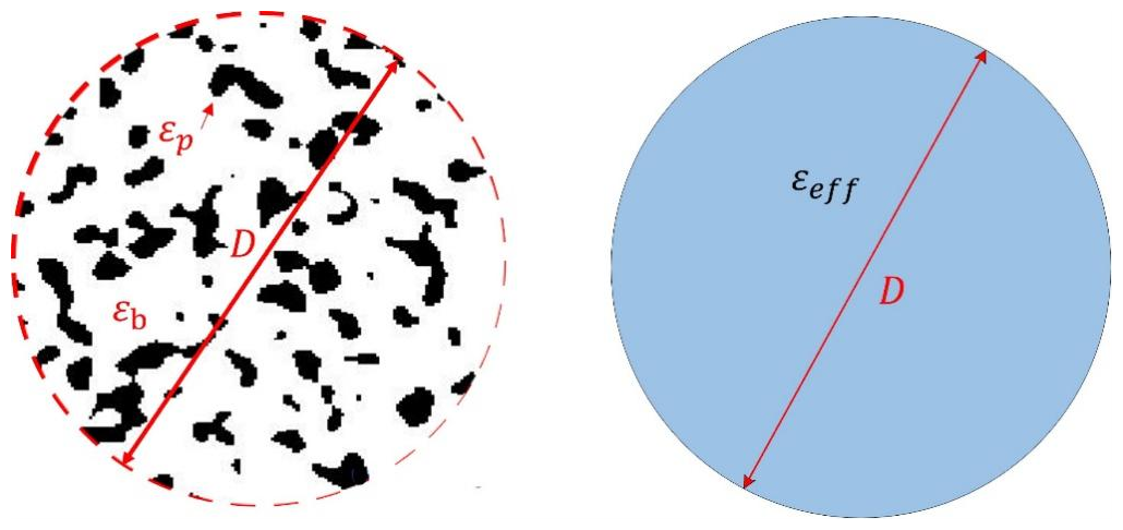
Figure 2 Problem A (left) and Problem B (right) are to be solved to evaluate effective permittivity.

Notice that the scattering and absorption from problem A are evaluated based on the average scattering and absorption from the computer-generated samples, which are obtained by the following:

$$\begin{array}{}\text{(13)}& {\displaystyle }{Q}_{\mathrm{abs}}^{\mathrm{A}}=〈{\displaystyle \frac{k}{\mathit{\pi }(D/\mathrm{2}{)}^{\mathrm{2}}}}\int {\mathit{ϵ}}^{\prime \prime }\left(\mathit{r}\right){|}^{\mathrm{2}}\mathrm{d}V〉\text{(14)}& {\displaystyle }{Q}_{\mathrm{scat}}^{\mathrm{A}}={\displaystyle \frac{\mathrm{1}}{\mathit{\pi }{\left(\frac{D}{\mathrm{2}}\right)}^{\mathrm{2}}}}\underset{\mathrm{0}}{\overset{\mathrm{4}\mathit{\pi }}{\int }}{\left|〈f_{pp}({\mathit{\theta }}_{\mathrm{s}},{\mathit{\varphi }}_{\mathrm{s}})〉\right|}^{\mathrm{2}}+{\left|〈f_{qp}({\mathit{\theta }}_{\mathrm{s}},{\mathit{\varphi }}_{\mathrm{s}})〉\right|}^{\mathrm{2}}\mathrm{d}\mathrm{\Omega }\end{array}$$

where the angular bracket 〈 〉 stands for a Monte Carlo ensemble average over the samples. E_int(r) is the internal field inside the mixture. f_pp and f_qp are the scattering amplitudes for p-polarized incident waves, with the scattered waves being p and q-polarized. In the linear polarization basis, p and q can both represent H and V. For the mixture of water and ice in the aquifer, in the L band, water has much higher dielectric loss. The absorption loss due to ice can thus be ignored.

In problem B, the scattering and absorption cross-section ($Q_{\mathrm{scat}}^{\mathrm{B}}$ and $Q_{\mathrm{abs}}^{\mathrm{B}}$) of a homogeneous sphere are solved. The sphere's diameter in Problem B is the same as the artificial boundary in Problem A. The calculations are based on the analytical Mie scattering theory. $Q_{\mathrm{scat}}^{\mathrm{B}}$ and $Q_{\mathrm{abs}}^{\mathrm{B}}$ are compared with $Q_{\mathrm{scat}}^{\mathrm{A}}$ and $Q_{\mathrm{abs}}^{\mathrm{A}}$. The real and imaginary parts of problem B are adjusted until $Q_{\mathrm{scat}}^{\mathrm{B}}=Q_{\mathrm{scat}}^{\mathrm{A}}$, $Q_{\mathrm{abs}}^{\mathrm{B}}=Q_{\mathrm{abs}}^{\mathrm{A}}$ The effective permittivity of the mixture is considered to be the value of the adjusted permittivity.

In this research, the aquifer's liquid water contents range from 5 % to 25 %. The values are obtained through full-wave simulation using bi-continuous media with 〈ζ〉=11 000 and b=5, which corresponds to an effective particle size of 1 mm. A detailed discussion of the simulation process can be found in Huang et al. (2024). In the dry firn, the density profile is converted into the permittivity profile from the work of Matzler (1996) and Tiuri et al. (1984). Results from the radiative transfer model combined with the aquifer effective permittivity were computed for the three sites of interest using the available in-situ data. The region above the aquifer is assumed to be dry snow.

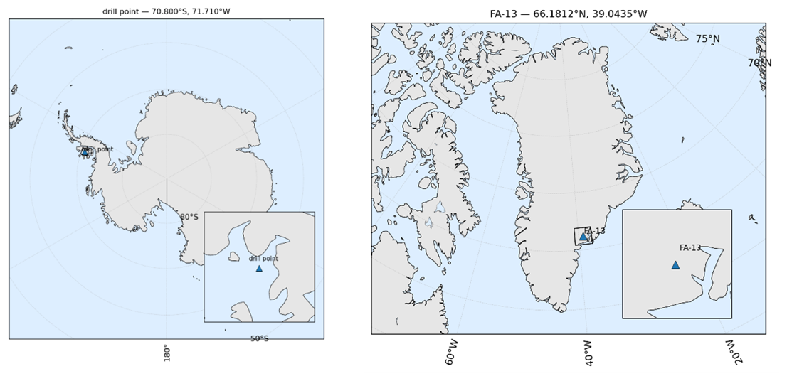
Figure 3 Borehole locations. The borehole is near the southeast coast of Greenland, and the borehole study on Antarctica is on the Wilkins Ice Shelf.

2.3 Investigation sites and data

The borehole locations are presented in Fig. 3 for Greenland and Antarctica, respectively. Both locations are close to the ocean coast. In situ measurements of physical temperature and firn density are plotted in Figs. 4–5 for the Greenland and Antarctic sites, respectively.

2.3.1 FA-13 Greenland

For the borehole of FA-13 in Greenland, the water table location (upper boundary of the aquifer) is available from the GPR echogram from the Accumulation Radar survey 2014 (Fig. B1). The FA-13 borehole was drilled and studied in 2013. The density and temperature profiles are plotted in Fig. 4. The temperature profile is obtained by directly interpolating the measured temperature.

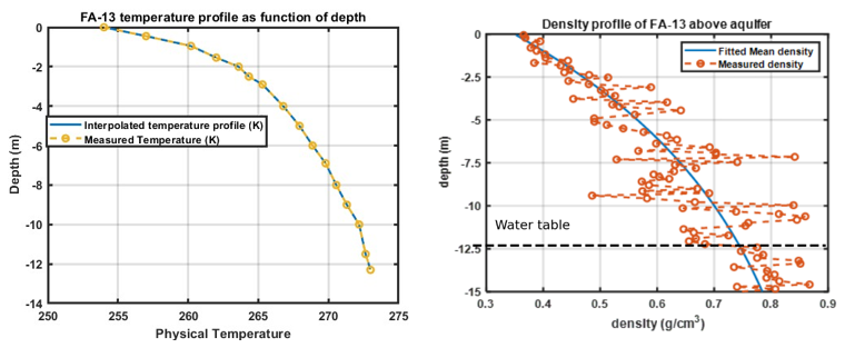
Figure 4 Temperature (left) and density profiles of FA13 from (Koenig et al., 2014; Montgomery et al., 2018). The measurements are taken on a scale of 0.5 m.

For FA-13, the temperature profile smoothly increases from 254 K at the firn-air interface to 273.15 K at the dry firn aquifer interface. This indicates that the top layer contains no liquid water before reaching the water table since the temperatures are below the melting point.

For the density profiles, the mean density is obtained by fitting a function of the shape $C-D\exp (-Ez)$ to the measured data. The density profiles show properties that are very different from those in the inner part of Greenland or Antarctica. Instead of having a slowly increasing mean density, as shown in the borehole measurements, where the mean profile reaches the critical density of 0.55 g cm⁻³ at about 5 m down from the surface, the mean density profiles in the aquifer regions increase dramatically. The density can be as high as 0.8 g cm⁻³ at a depth of 12 m, as shown in the case of FA13.

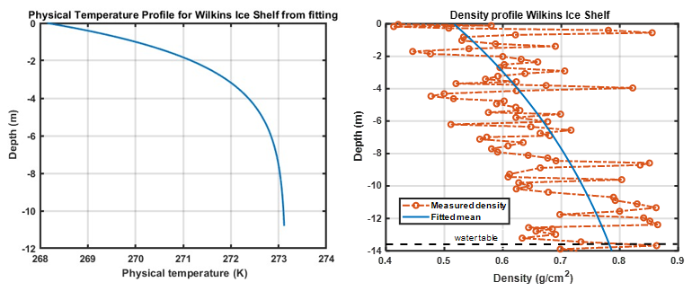
Figure 5 Density profile from the borehole in Wilkins Ice Shelf and the fitted temperature connecting surface and water table. The temperature profile is composed of the surface temperature and the water table depth.

2.3.2 Wilkins Ice Shelf, Antarctica

Density measurement and water table location are available from the Wilkins Ice Shelf's borehole (Fig. 5). The physical temperature in the borehole is not publicly available. A fitting method is used to obtain the temperature profile, as the radiative transfer model needs a temperature profile as input; a fitted temperature profile is generated using the surface temperature and water-ice mixture profile. For the Wilkins location, the function $T\left(z\right)=A-B\exp \left(Cz\right)$ is used to connect the surface and aquifer temperatures. In the forward simulation, the physical temperature in the dry firn region is obtained as follows: The surface temperature of the Wilkins Ice Shelf borehole location is chosen as −5 °C given that the nearest valid surface temperature is in the range of −3 to −10 °C in mid May. The temperature profile follows an exponential-like function as $T\left(z\right)=\mathrm{273.15}-\mathrm{5}\exp \left(Cz\right)$. The C value can be obtained by forcing $T\left(z=-\mathrm{13.5}\right)-\mathrm{273.15}<\mathrm{10}\wedge -\mathrm{3}$. The results show that setting b, being one-fifth of the water table depth, which is b=2.65 m, would fit the need. Given that the subsurface temperature is more stable as observed from FA-13 (Koenig et al., 2014), a better approach to estimate the temperature profile is needed in the future retrieval work. Mean density of the Wilkins Ice Shelf borehole is obtained from the same method used for FA-13. Density fluctuates much more strongly than that in the FA-13 borehole. The magnitude of density fluctuations is also much higher than that in the accumulation zone of Greenland and Antarctica. In terms of the density variations, the density fluctuates dramatically from the mean value due to the presence of refrozen ice structures in these regions.

2.3.3 Other Parameters

The water level for all the boreholes used in this research is presented in Table 1 The water table positions of FA-13 and Wilkins Ice Shelf are from the borehole measurements.

Table 1 Water Table levels for all locations.

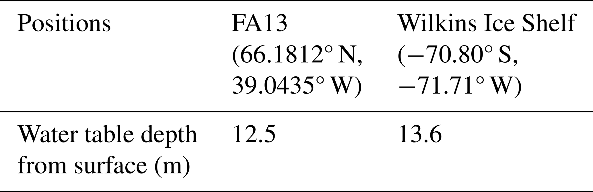
Figure 6 provides the effective permittivity of the aquifer (ice water mixture) as a function of liquid water content. The three curves correspond to different shapes of inclusions, such as spheres, bicontinous media(shapeless), and needles. Maxwell-Garnett mixing formula is used to evaluate the sphere and needle cases, while the bicontinous media is evaluated using the method in Sect. 2.2. As shown in the plots, both the real and imaginary parts of the effective permittivity values increase with respect to the increase in liquid water content. However, the speed of the increase is very different.

Medium with sphere inclusions has the lowest permittivity values in both the real and imaginary parts. The increments are also the smallest in all three cases. For the real and imaginary parts, the values increase from 3.65 to 5.97 and from 0.006 to 0.045 as water content increases from 0.05 to 0.25. Needle inclusion has the largest values and the largest increments. The values increase from 4.8 to 12.4 and from 0.17 to 1.01 for the real and imaginary parts, respectively. The bicontinous media is between the two, with an increase from 3.75 to 9.5 and 0.017 to 0.42 for the real and imaginary parts, respectively. This indicates that effective permittivity depends highly on the shape of the inclusion. A good geometry description of the mixture in permittivity modelling is important in modelling the emission.

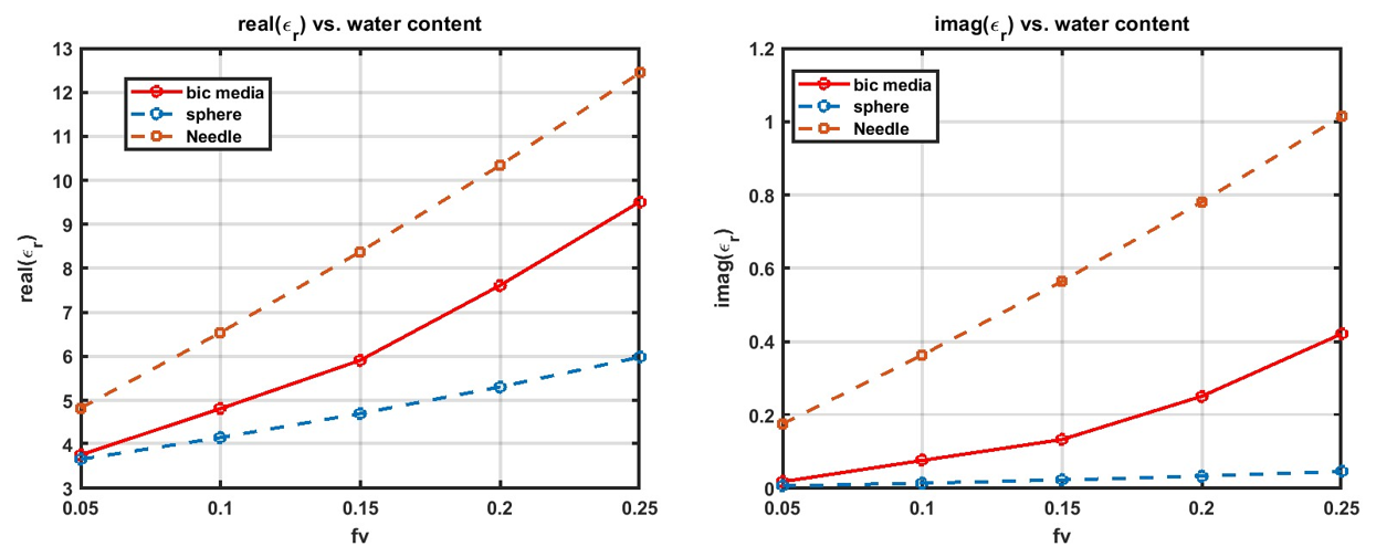
Figure 6 Effective permittivity values through the full wave bi-continuous media and spheres.

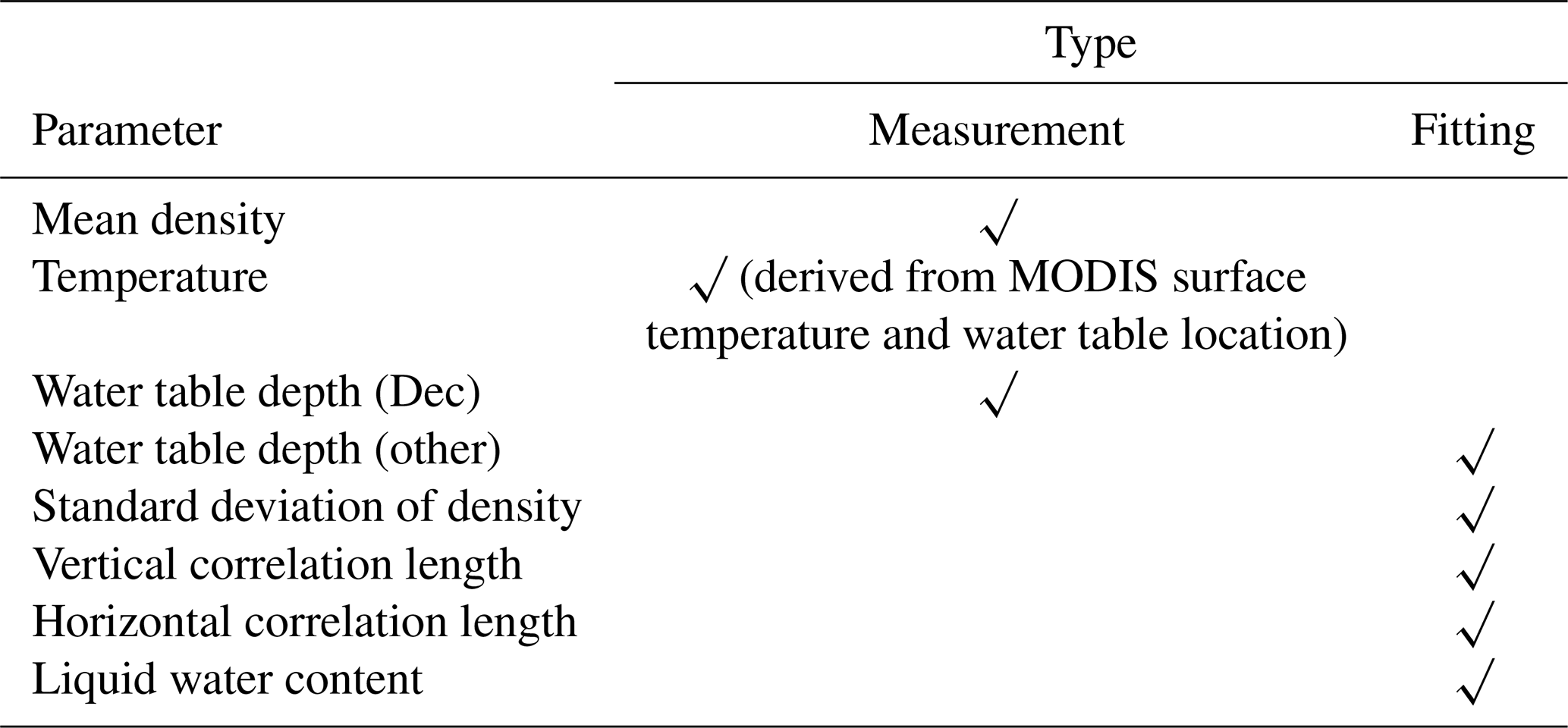
In the simulation process, the input parameters are either from measurements or from empirical fitting. They are summarized in the Tables 2 and 3.

Table 2 Summary for the parameters used for forward simulation of time series at FA-13

Table 3 summary for the parameters used for forward simulation of time series at Wilkins Ice Shelf.

3 Results

3.1 Forward simulation of SMAP brightness temperatures

Time series results for FA13 are provided in Fig. 7. The numerical simulation is performed for five points in the time series from 7 December 2015, to early April 2016. Melting events occur in the later days of April. Thus, the latter part of the time series is not discussed. The parameters we used for the five-time series points are listed in Table 4.

The temperature profiles and water table location are provided in the top two plots in Fig. 7. At the beginning of the time series, early December 2015, the water table is assumed to be half of the depth of April 2016. As the spring of 2016 came, the water table gradually decreased to its lowest level of 12.3 m below the surface. Notice that the change of water table is a hypothesis, as it is observed that the water table of mountain glacier aquifers would decrease seasonally (van den Akker et al., 2025). Further research is needed to quantify the seasonal changes in the water table. Regarding the temperature profile, at each time point, the temperature profile in April is “squeezed” to fit the temperature at the dry firn aquifer interface. The temperature–depth profile was rescaled by applying a uniform scaling factor to the depth axis, while preserving the temperature values. The scaling factor was determined such that the deepest point of the profile coincides with the water table depth.

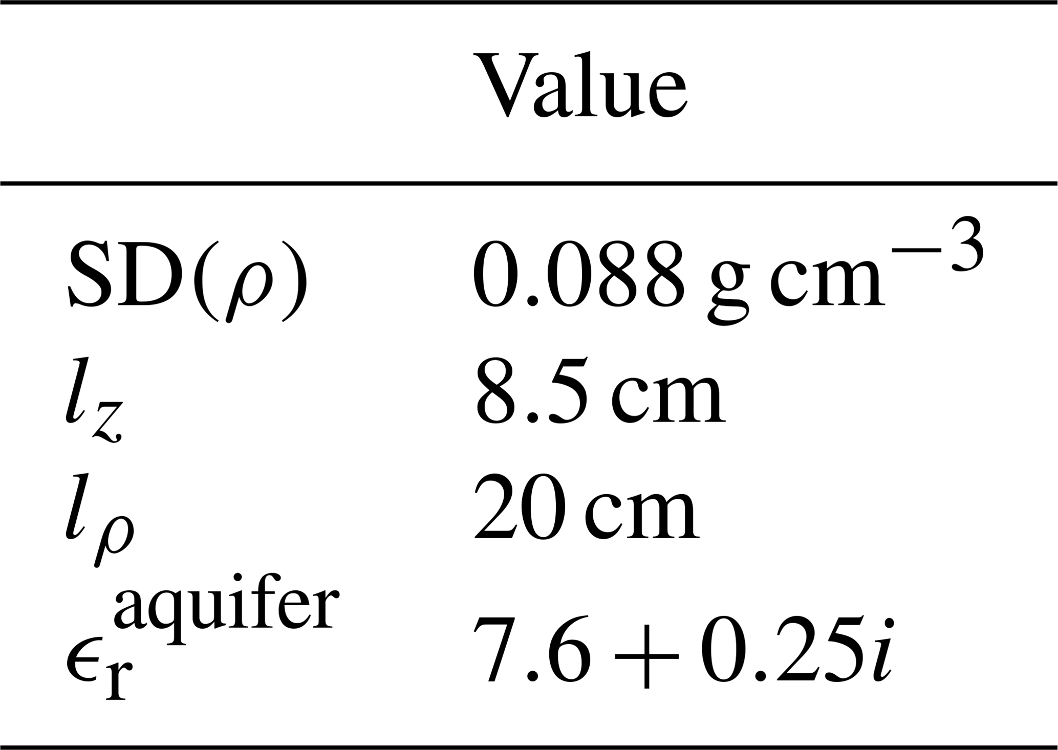
The mean density profile is used as input for the iterative approach. The density fluctuation properties are used as a tuning parameter. The variance of density and vertical correlation length is first tuned such that the V-pol brightness temperature is close to the observations. Then the horizontal correlation length is tuned to adjust the difference between V and H-pol. Although the properties of density fluctuation can be obtained from the measured profile, tuning parameters are used instead. This is because the density measurement is usually performed over the drilled ice core samples. Such samples are usually tens of centimeters long, and measuring the density of the sample would unavoidably smooth out the density fluctuations and suppress the spatial variations within the sample. Radiative transfer theory uses the statistical properties as the inputs, profiles from measurement only represent the given location, but cannot provide statistical information for the radiometer resolution area. For this case, a density standard deviation of 0.088 g cm⁻³ is used with vertical and horizontal correlation lengths of 8.5 and 20 cm, respectively. The statistical properties of the density fluctuations are considered to be homogeneous from the top to the bottom of the dry firn.

The firn aquifer permittivity is set as 7.6 + 0.25i, corresponding to 20 % of liquid water content for the water and ice mixture in the firn aquifer. The results are obtained from the full wave simulations using bi-continuous media, as in Fig. 6 In the time series simulations, the permittivity of the region below the water table is assumed to be the same for all the data points where forward simulation is performed.

With the given density parameters, the simulated time series matches the measured brightness temperatures for both V and H polarizations. The overall standard deviation is around 3 K. A detailed analysis of the contribution to the brightness temperature reduction in terms of reflectivity is provided in Table 4. In the analysis, the depth of the water table decreases from 6 m in early December to 12.3 m in early April. As indicated in the table, the reduction from the aquifer interface decreases. This can be explained by the change in the firn permittivity adjacent to the aquifer. The permittivity of dry firn above the aquifer changes from 2.25 to 2.65. The permittivity difference between the aquifer and the dry firn is thus decreased. A major reduction in the emission is due to the density fluctuations in the dry firn. As the depth increases, dry firn volume increases, leading to an increase in reflection numbers due to density fluctuations. The brightness temperature reductions can be explained by the increase in the dry firn volume. Notice that when modelling the time series, the mean density profile is fixed. The change of the water table would “truncate” the mean density profile that holds the variations.

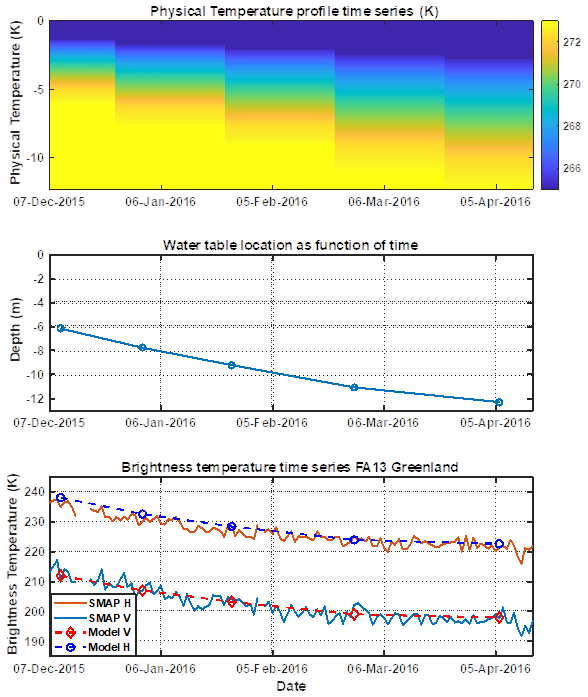
Figure 7 Time series for FA13 from winter 2015 to summer 2016. The match-up stopped in early April 2016.

Table 4 FA-13 parameters for the 5 points of time series in forward simulations of TB for Greenland. TB reduction evaluates the difference between emissivity = 1, direct emission from the aquifer, and the TB modelled time series. This is to evaluate how much brightness is reduced due to the dry firn above the aquifer.

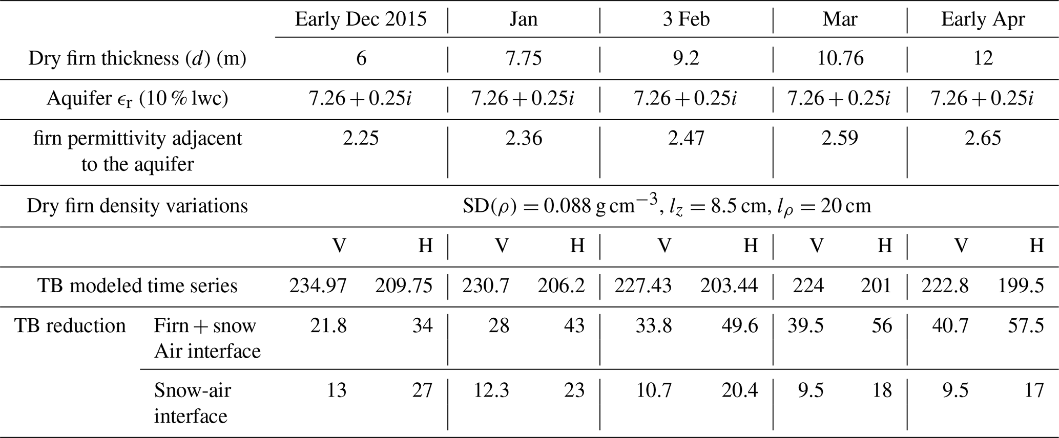
Table 5 Density fluctuation parameters and the aquifer permittivity for the forward match-up results of FA-13 in Fig. 7.

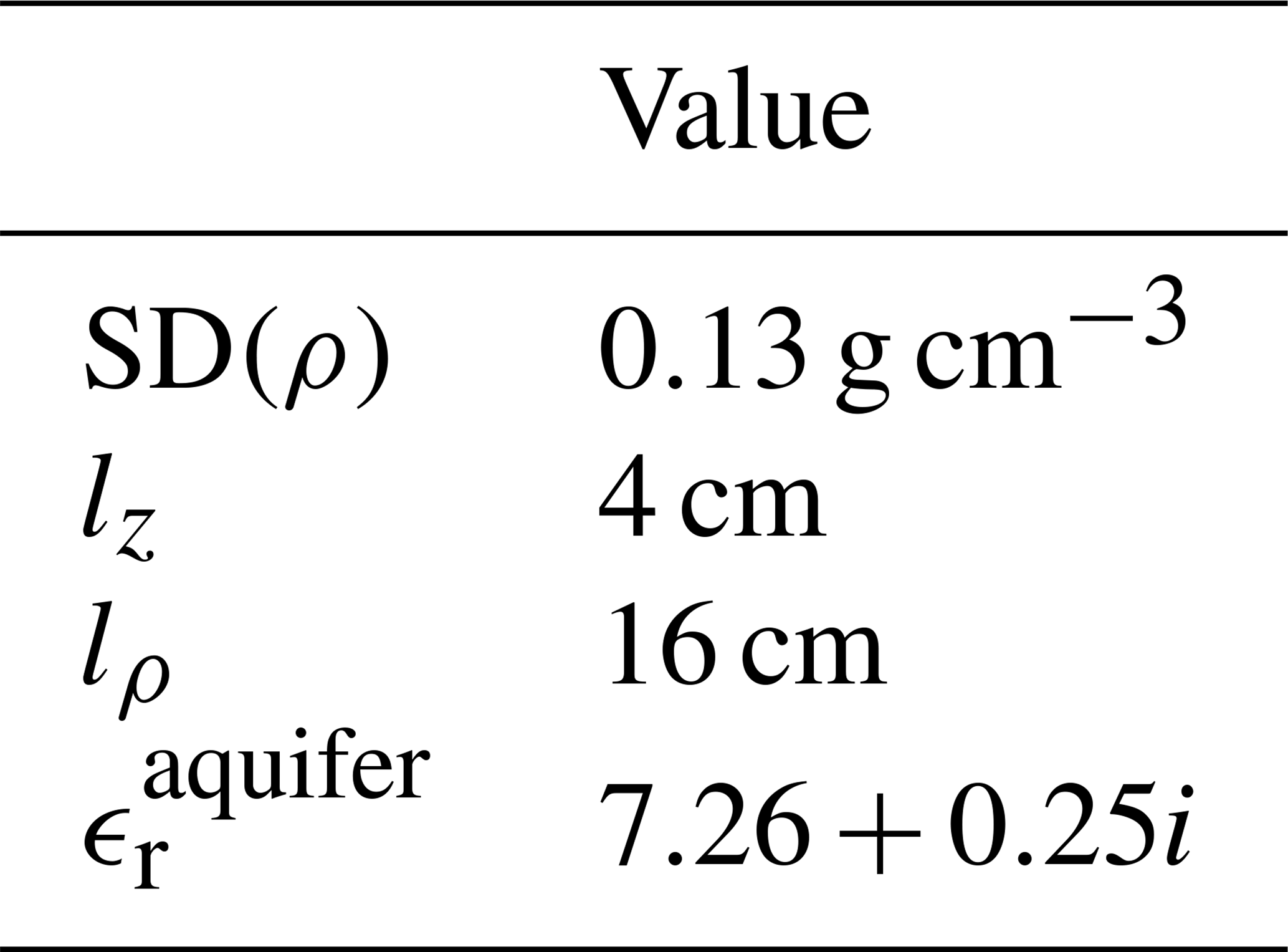
To simulate the brightness temperature for the time series points, the water table location is adjusted as shown in Fig. 8. The properties are used to characterize the density fluctuation properties to match up both the V and H-pol brightness temperatures: SD(ρ)=0.13 g cm⁻³, l_z=4 cm, l_ρ=16 cm. The forward simulated results are plotted together with the SMAP measurements. The simulated results reflect the decrease in brightness temperature, assuming the changes are purely due to the changes in the water table.

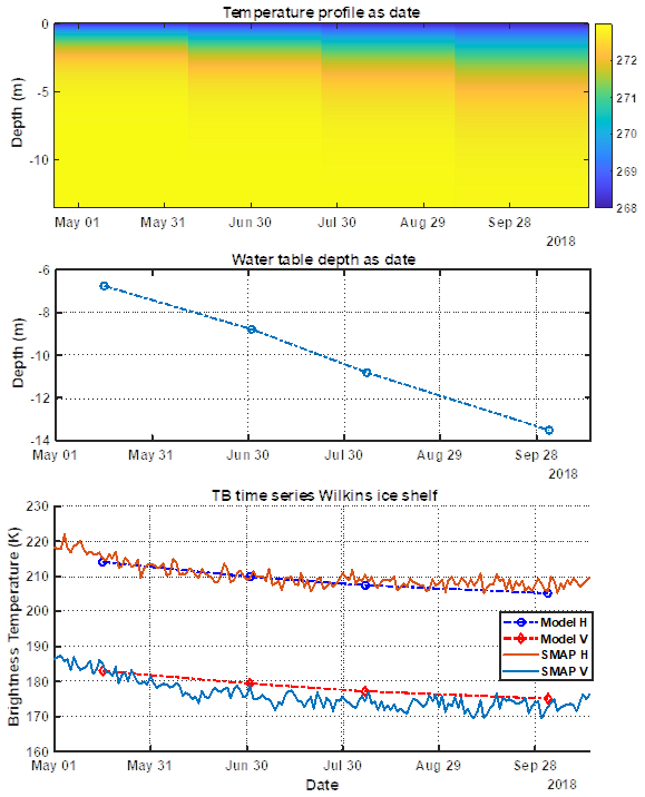
Figure 8 Brightness temperature time series data and forward modelled results over the borehole pixel in Wilkins Ice shelf, 2018.

Table 6 Density fluctuation parameters and the aquifer permittivity for the forward match-up results in Fig. 8 for the Wilkins Ice shelf.

3.2 Parameter Sensitivity Analysis

In this section, the FA-13 site is used as an example to analyse the sensitivity of brightness temperature to liquid water content in the firn aquifer. Brightness temperatures at 40° observation angle are calculated for different aquifer water table depths and liquid water content.

Brightness temperatures as a function of liquid water content in the aquifer are plotted in Fig. 8. Each subfigure corresponds to a different water table depth from the surface, starting from 6.15 m (half of the maximum depth) to 12.3 m (maximum depth) below the firn-air interface. When performing the simulations, the volume scattering from the dry firn is characterized using. SD(ρ)=0.088 g cm⁻³, l_z=0.085 m, l_ρ=0.2 m, which is the same as the parameters used for the time series match-up.

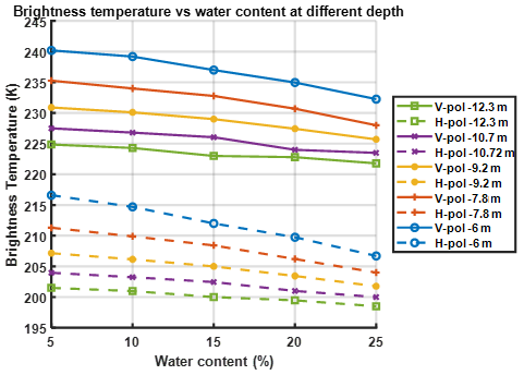
Figure 9 Brightness temperature as a function of liquid water content in the firn aquifer with the water table at different depths.

All brightness temperature plots show a decreasing trend with the increased liquid water content inside the aquifer. However, the impact of liquid water content decreases as the water table depth increases. When the water table is 6.15 m below the surface, the brightness temperatures decrease by 8 K in V-pol and 10 K in H-pol as the liquid water content increases from 5 % to 25 %. Then, for water table depth at 7.68, 9.23, and 10.22 m, the brightness temperature decreased by 7.2, 5.4, and 4 K for V-pol, and 7.3, 5.4, and 4 K for H-pol, respectively. The changes in brightness temperature finally become 3 and 3.3 K when the aquifer water table depth is 12.3 m. This phenomenon happens due to two factors: (1) The decrease of the permittivity contrast between the dry firn and aquifer. The permittivity of the aquifer is fixed as the liquid water content is fixed. However, the firn permittivity increases when depth increases due to the increase in mean density. (2) The second factor is the increase in volume scattering in the dry firn region – the total volume scattering increases as more scatterers are included due to the increase in depth.

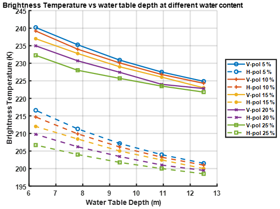
Figure 10 Brightness temperature changes as a function of water table depth at different fixed liquid water contents.

Brightness temperature changes as a function of depth are plotted in Fig. 10 for fixed aquifer liquid water content. For all the cases, as the water table depth changes from 6.15 to 12.3 m, the decrease in brightness temperatures is usually more than 10 K for both V and H-pol. This decrease is mainly due to the increased dry firn volume and thus the increased volume scattering. As the water table becomes deeper, the permittivity difference between dry firn and aquifer gets smaller. This would increase the emissivity from the aquifer. However, such an increase is overwhelmed by the increase in dry firn volume as indicated by the decreasing trend of brightness temperature. The most significant drop in brightness temperature happens for a liquid water content of 5 %. The brightness temperature drops from 240 to 225 K for V-pol and from 216.6 to 201.5 K. At 25 % liquid water content in the aquifer, the brightness temperature drops about 10K when the water table changes from 6.15 to 12.3 m. The dynamic range decreases as the liquid water content increases. This is due to the increase in multiple reflections happening between the top and bottom interfaces of the dry firn region.

The combined effects of water content and water table depths are presented in this section with the following two combinations: (1) Increasing liquid water content in the aquifer as the water table deepens. (2) Decreasing the liquid water content in the aquifer as the water table deepens. It is unclear how the liquid water content would change according to the seasonal changes. These results illustrate the two possible trends of liquid water content from winter to spring. The simulation results would provide a physical intuition for interpreting the time series data.

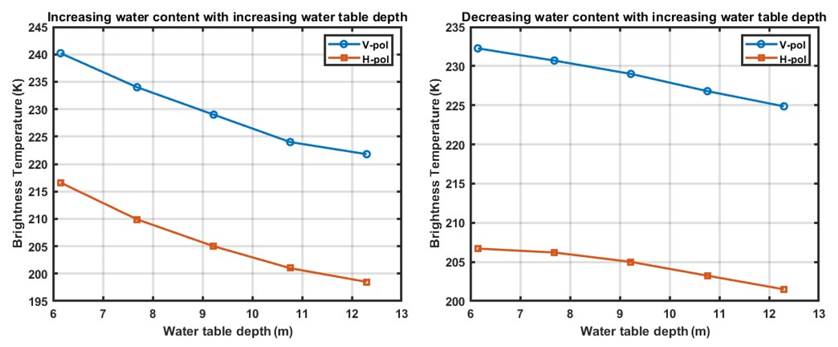
Figure 11 Brightness temperature changes as a function of depth with the liquid water content in an increasing and decreasing order. For the left-hand side figure, liquid water content increases from 5 % to 25 % from 6.2 to 12.3 m water table depth. For the right-hand side figure, liquid water content decreases from 25 % to 5 % as the water table depth increases.

Figure 11 plots brightness temperatures for the cases when the liquid water content increases and decreases with respect to the water table depth. The left figure shows the case where liquid water content increases as water table depth decreases. The first case where water content decreases assumes that the aquifer is very wet after the melt season, then it dries up as the low temperature at the surface gradually takes heat out of the firn. The second case, where water content increases as the water table lowers, assumes that water gradually accumulates in a deeper position. Noticing that the temporal changes of the firn aquifer are only assumptions, their correctness would need to be justified or falsified by future direct measurements of the firn aquifer. The figure indicates that the decrease in water table depth, when accompanied by an increase in water content, results in a more pronounced reduction in brightness temperature than that caused by the decrease in water table depth alone. The overall effect contributed to a 20 K reduction in V-pol and an 18 K reduction in H-pol. On the other hand, for the right-hand side figure, the decreasing water content counters the effects of the increasing depth. The overall effects decrease the change of brightness temperature with respect to depth. The V-pol decreases by 7 K, and the H-pol decreases by only about 5 K in total. This implies that the decreasing of SMAP brightness temperature is a complex process; decreased water table location and changes in the firn aquifer liquid water content can both contribute to such changes.

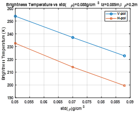
Figure 12 Brightness temperature changes with respect to SD(ρ) V-pol and H-pol both decrease as the value of SD(ρ) Increases.

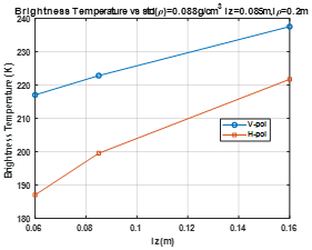
Figure 13 Brightness temperature changes with respect to l_z. With smaller l_z the reduction in brightness temperature gets stronger.

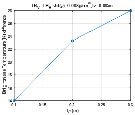
Figure 14 The brightness temperature difference between V and H-pol with respect to the horizontal correlation length.

The parameters of SD(ρ)l_z and l_ρ are the parameters that control the properties of volume scattering in the dry firn. The parameters of SD(ρ) and l_z are determining the strength of each reflection and the number of reflections in a unit length in the z-direction. As shown in Figs. 12 and 13, the increase of SD(ρ) and the reduction of l_z would reduce the brightness temperature in both V and H-pol. The horizontal correlation length controls the difference between V-pol and H-pol emission, as shown in Fig. 14. The increase of l_ρ would make the media behave more likely to layers as a longer horizontal correlation length means the media is homogeneous in a longer horizontal area(layers have l_ρ=∞), making the V-pol and H-pol more different from each other. Smaller l_ρ values allow the V-pol and H-pol to be coupled to each other.

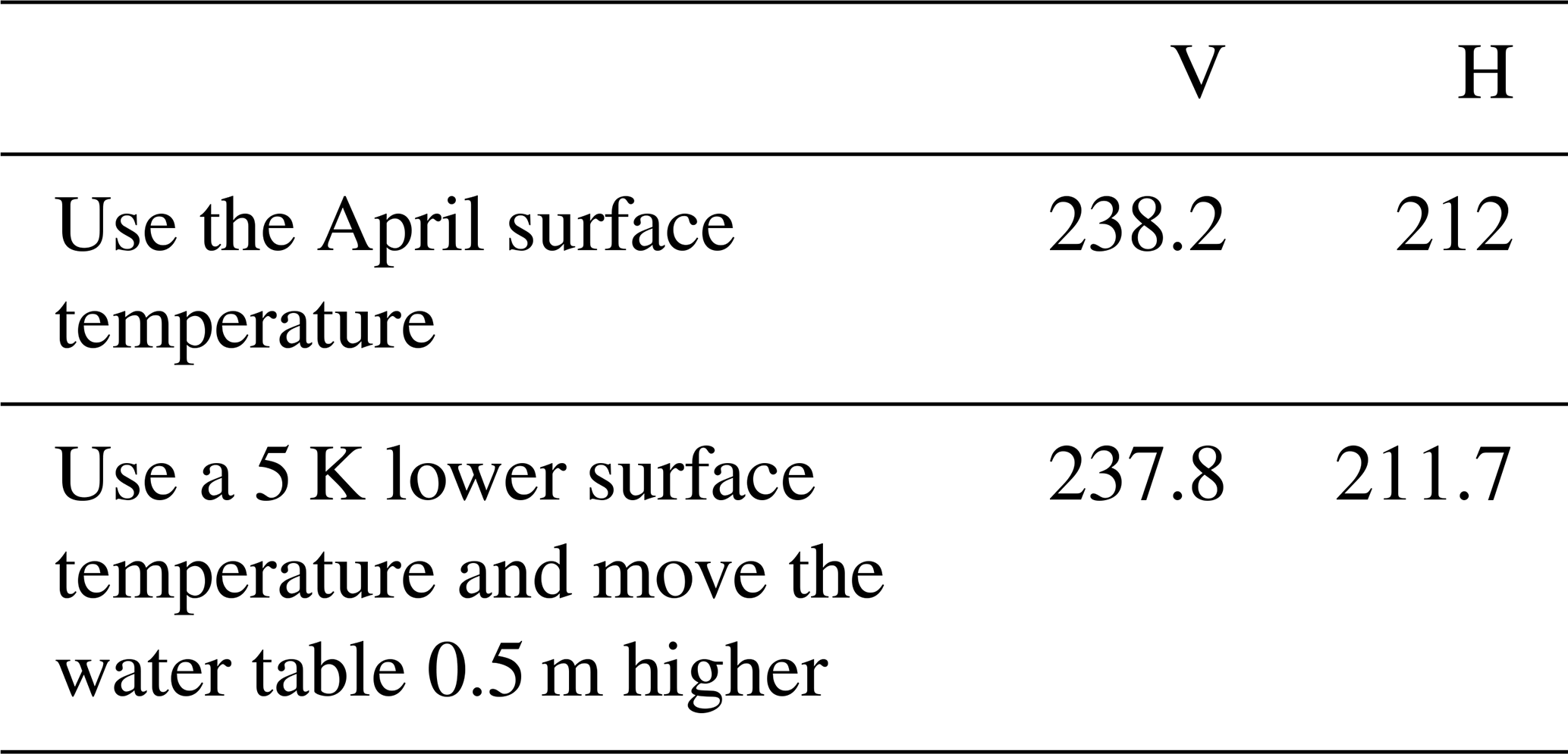
The uncertainty in the surface temperature could affect the parameters used in the forward simulation of the brightness temperature. For example, the surface temperature is changed by 5 K in the FA-13 in December. Keeping the same density properties, by changing the water table depth 0.5 m higher, the model predicted TB would be within 1 K of the observed results. The question of how the seasonal temperature change affects the water table location of the aquifer is a more complicated scientific problem beyond the scope of this paper. The question shall be answered in future studies.

Table 7 Model results by changing surface temperature.

4 Discussion

The radiative transfer model provided in this paper has shown its ability to predict the time series brightness temperature changes from winter to early spring before surface melting starts for both the V and H-pol time series brightness temperatures. This model potentially provides an explanation for the difference between V and H polarized brightness temperature data. For future work on the retrieval of liquid water content for the top region of the aquifer, this model enables the use of both V and H-pol measurements. The radiative transfer model in this work provides a tool that can simulate the observed brightness temperature and help with the retrieval of the firn aquifer properties in future work. Some of the inputs are tuned empirically (e.g., density fluctuation parameters) either because the measurements are not available or the parameters are not provided on the microwave scale. These parameters will be used as empirical inputs to serve the retrieval of firn aquifer properties.

Comparing the time series results from the aquifer, it can be observed that the brightness temperatures from Wilkins Ice Shelf are about 10 K lower than the TB observed over southeast Greenland. Our analysis provides one of the possible explanations that dry firn above the aquifer of the Wilkins Ice Shelf has a higher density variation. The selection of higher density variation than Greenland can be justified by the comparison of density profiles in the first section.

In Fig. 7, the time series is simulated based on the assumption of unchanged liquid water content in the firn aquifer and density parameter with a changing depth of the firn aquifer. In Fig. 11 The simulated brightness temperatures are based on the same density parameters but include changes in the liquid water content. If the liquid water content in the aquifer has a decreasing trend, the brightness temperature from December to April is much less than the case when the liquid water content increases with time, and the change in Fig. 7. This shows that the change in the liquid water with respect to time can also influence the time series brightness temperature at the L-band.

The model used in this paper has assumed a dry condition above the aquifer; when there is wetness above, the current model cannot handle it. Figure C1 shows the temperature profiles measured in the boreholes of FA 15-1 and -2. This is different from the case in FA-13, where the temperature profiles reach 0° C at the position of the water table, the temperature profiles in these two boreholes reach 0° C at a much shallower position than the water table. As a result of this, there is a “warm” region. The high temperatures in these regions allow the existence of liquid water. These regions are called unsaturated zones in the work of Miller et al. (2017). The thermal emission from these regions is much more complicated since the liquid water content in these regions will affect the contribution from the aquifer. With higher liquid water, radiometers may not see emissions from the aquifer. Further studies are needed to understand the loss factor of the unsaturated zone, where the media is a three-phase mixture of air, ice, and water. A method of separating the regions with and without unsaturated zones is needed to apply the physical model presented in this paper.

One of the features that could affect the emission is the mean density profile of the firn. The mean profile affects both the reflections due to the dry firn and the interface of dry firn and aquifer. To evaluate its effects, several different mean density profiles need to be used in the simulation. However, the in-situ data is very limited. Another approach is to use the simulated profiles. The Community Firn Model (Stevens et al., 2021) has been updated lately to better deal with the percolation facets of the polar ice sheet. However, the simulated mean density profile reaches the ice density at a much shallower depth than the measured mean density, which does not correctly reflect the truth. The modelled results need to be further improved before using them to analyse the mean density profile effects.

As discussed earlier in the paper, the variation properties of the dry firn affect the emission. These properties would better be characterized before retrieving the properties related to the firn aquifer (e.g., water table depth, liquid water content). As higher frequency microwaves are more sensitive to the near-surface properties, data from the AMSR-2 multi-frequency radiometer (C, X, Ku, and Ka) would potentially help with achieving such goals.

5 Conclusions

A physical model for the L-band microwave thermal emission of a firn aquifer region was reported. The radiative transfer model formulation is solved iteratively to include scattering contributions within the inhomogeneous dry firn region. The reflections of thermal emission are considered due to the firn-aquifer interface, air-firn interface, and density fluctuations in the dry firn region. A full-wave approach was used to simulate the effective permittivity of the aquifer. The 3D structure of the modeled density fluctuations allowed both V and H-polarized SMAP measurements to be reproduced using a single set of parameters and to reproduce SMAP time series data over the Greenland coast and Wilkins Ice Shelf, Antarctica.

Sensitivity analyses further show that the L-band brightness temperature varies more strongly with aquifer liquid water content when the water table is closer to the surface. This is shown in Fig. 10 by the reduced sensitivity to liquid water content as the water table becomes deeper: The dynamic range reduces from 8 to 3 K as the water table decreases from 6 to 12.5 m. This indicates a possible better result in the future retrieval work compared to deeper aquifer cases. It is also shown that both the firn aquifer depth and the liquid water content in the firn aquifer would affect the time series brightness temperature at the L-band. The method provides a tool for the radiometry study of the firn aquifer. The brightness temperatures due to different combinations of density properties and firn aquifer properties can be estimated through the model. The method can also be extended to explain the passive microwave measurements at other frequencies. The model also provides a theoretical basis for potentially retrieving firn aquifer liquid water content using passive microwave data. Look-up tables can be generated and used for future retrieval.

The SMAP brightness temperature time series is also modelled by the radiative transfer model with the hypothesis of a decreasing water table from December to April. The hypothesis itself needs to be further validated by the direct observations of water table location over the seasons.

Appendix A: Iterative solution of radiative transfer equations

The first step is to convert the equations from differential-integral form into pure integral form. For the upward brightness temperature, the variable z is changed into z^′, then the term $\exp \left(-\sec \mathit{\theta }{\int }_{z^{\prime }}^{\mathrm{0}}\overleftrightarrow{{\mathit{\kappa }}_{\mathrm{e}}}\left(\mathit{\theta },z^{\prime \prime }\right)\mathrm{d}{z}^{\prime \prime }\right)$ is multiplied by both sides of the equation. For upward-going brightness temperatures, integration was performed on z^′ ranges from $z{}^{\prime }=-d$ to $z{}^{\prime }=z$. The equation is thus changed into:

$$\begin{array}{}\text{(A1)}& \begin{array}{rl}& {\int }_{-d}^z\cos {\mathit{\theta }}_i{\displaystyle \frac{d}{\mathrm{d}{z}^{\prime }}}{\mathit{T}}_{\mathrm{u}}\left(\mathit{\theta },z^{\prime }\right)\exp \left(-\sec \mathit{\theta }{\int }_{z^{\prime }}^{\mathrm{0}}\overleftrightarrow{{\mathit{\kappa }}_{\mathrm{e}}}\left(\mathit{\theta },z^{\prime \prime }\right)\mathrm{d}{z}^{\prime \prime }\right)\\ & =\cos {\mathit{\theta }}_i{\mathit{T}}_{\mathbf{u}}\left(\mathit{\theta },z\right)\exp \left(-\sec \mathit{\theta }{\int }_z^{\mathrm{0}}{\overleftrightarrow{\mathit{\kappa }}}_{\mathrm{e}}\left(\mathit{\theta },z^{\prime \prime }\right)\mathrm{d}{z}^{\prime \prime }\right)\\ & -\cos {\mathit{\theta }}_i{\mathit{T}}_{\mathrm{u}}\left(\mathit{\theta },z^{\prime }=-d\right)\exp \left(-\sec \mathit{\theta }{\int }_{-d}^{\mathrm{0}}{\overleftrightarrow{\mathit{\kappa }}}_{\mathrm{e}}\left(\mathit{\theta },z^{\prime \prime }\right)\mathrm{d}{z}^{\prime \prime }\right)\\ & -{\int }_{-d}^z\mathrm{d}{z}^{\prime }\cos {\mathit{\theta }}_i{\mathit{T}}_{\mathbf{u}}\left(\mathit{\theta },z^{\prime }\right)\left[\sec \mathit{\theta }\overleftrightarrow{{\mathit{\kappa }}_{\mathrm{e}}}\left(\mathit{\theta },z^{\prime }\right)\right]\\ & \exp \left(-\sec \mathit{\theta }{\int }_{z^{\prime }}^{\mathrm{0}}\overleftrightarrow{{\mathit{\kappa }}_{\mathrm{e}}}\left(\mathit{\theta },z^{\prime \prime }\right)\mathrm{d}{z}^{\prime \prime }\right)\end{array}\end{array}$$

Integrate the left-hand side by parts and cancel out the same terms on both sides of the equation. The formatted equation becomes the following:

$$\begin{array}{}\text{(A2)}& \begin{array}{rl}{\mathit{T}}_{\mathbf{u}}\left(\mathit{\theta }z\right)& ={\mathit{T}}_{\mathrm{u}}\left(\mathit{\theta },z^{\prime }=-d\right)\\ & \exp \left(-\sec \mathit{\theta }{\int }_{-d}^z\overleftrightarrow{{\mathit{\kappa }}_{\mathrm{e}}}\left(\mathit{\theta },z^{\prime \prime }\right)\mathrm{d}{z}^{\prime \prime }\right)\\ & +\sec \mathit{\theta }{\int }_{-d}^z{\mathit{\kappa }}_{\mathrm{a}}\left(z^{\prime }\right)T_{\mathrm{0}}\left(z^{\prime }\right)\\ & \exp \left(-\sec \mathit{\theta }{\int }_{z^{\prime }}^z\overleftrightarrow{{\mathit{\kappa }}_{\mathrm{e}}}\left(\mathit{\theta },z^{\prime \prime }\right)\mathrm{d}{z}^{\prime \prime }\right)\mathrm{d}{z}^{\prime }\\ & +\mathit{S}\left(\mathit{\theta }z\right)\end{array}\end{array}$$

where S_u(θz) is the term that accounts for the scattering:

$$\begin{array}{}\text{(A3)}& \begin{array}{rl}& S\left(\mathit{\theta },z^{\prime }\right)=\sec \mathit{\theta }{\int }_{-d}^z\mathrm{d}{z}^{\prime }\exp \left(-\sec \mathit{\theta }{\int }_{z^{\prime }}^z\overleftrightarrow{{\mathit{\kappa }}_{\mathrm{e}}}\left(\mathit{\theta },z^{\prime \prime }\right)\mathrm{d}{z}^{\prime \prime }\right)\\ & {\int }_{\mathrm{0}}^{\frac{\mathit{\pi }}{\mathrm{2}}}\mathrm{d}{\mathit{\theta }}^{\prime }\sin {\mathit{\theta }}^{\prime }[\mathit{P}\left(\mathit{\theta },{\mathit{\theta }}^{\prime },z^{\prime }\right){\mathit{T}}_{\mathrm{u}}\left({\mathit{\theta }}^{\prime },z^{\prime }\right)\\ & +\mathit{P}\left(\mathit{\theta },\mathit{\pi }-{\mathit{\theta }}^{\prime },z^{\prime }\right){\mathit{T}}_{\mathrm{d}}\left({\mathit{\theta }}^{\prime },z^{\prime }\right)]\end{array}\end{array}$$

Using a similar technique, the downward brightness temperature in the dry firn region can be obtained by multiplying the term. $\exp \left(-\sec \mathit{\theta }{\int }_{-d}^{z^{\prime }}\overleftrightarrow{{\mathit{\kappa }}_{\mathrm{e}}}\left(\mathit{\theta },z^{\prime \prime }\right)\mathrm{d}{z}^{\prime \prime }\right)$ and integrate z^′ from $z^{\prime }=z$ to $z{}^{\prime }=\mathrm{0}$. After some math, the downward brightness temperature can be simplified into the following:

$$\begin{array}{}\text{(A4)}& \begin{array}{rl}{\mathit{T}}_{\mathbf{d}}\left(\mathit{\theta }z\right)& ={\mathit{T}}_{\mathbf{d}}(\mathit{\theta },\mathrm{0})\exp \left(-\sec \mathit{\theta }{\int }_z^{\mathrm{0}}\overleftrightarrow{{\mathit{\kappa }}_{\mathrm{e}}}\left(\mathit{\theta },z^{\prime \prime }\right)\mathrm{d}{z}^{\prime \prime }\right)\\ & +\sec \mathit{\theta }{\int }_z^{\mathrm{0}}{\mathit{\kappa }}_{\mathrm{a}}\left(z^{\prime }\right)T_{\mathrm{0}}\left(z^{\prime }\right)\\ & \exp \left(-\sec \mathit{\theta }{\int }_z^{z^{\prime }}\overleftrightarrow{{\mathit{\kappa }}_{\mathrm{e}}}\left(\mathit{\theta },z^{\prime \prime }\right)\mathrm{d}{z}^{\prime \prime }\right)\mathrm{d}{z}^{\prime }\\ & +\mathit{W}\left(\mathit{\theta }z\right)\end{array}\end{array}$$

where:

$$\begin{array}{}\text{(A5)}& \begin{array}{rl}W\left(\mathit{\theta },z\right)=& \sec \mathit{\theta }{\int }_z^{\mathrm{0}}\mathrm{d}{z}^{\prime }\exp \left(-\sec \mathit{\theta }{\int }_z^{z^{\prime }}\overleftrightarrow{{\mathit{\kappa }}_{\mathrm{e}}}\left(\mathit{\theta },z^{\prime \prime }\right)\mathrm{d}{z}^{\prime \prime }\right)\\ & {\int }_{\mathrm{0}}^{\frac{\mathit{\pi }}{\mathrm{2}}}\mathrm{d}{\mathit{\theta }}^{\prime }\sin {\mathit{\theta }}^{\prime }[\overleftrightarrow{P}\left(\mathit{\pi }-\mathit{\theta },{\mathit{\theta }}^{\prime }\right){\mathit{T}}_{\mathrm{u}}\left({\mathit{\theta }}^{\prime },z\right)\\ & +\overleftrightarrow{P}\left(\mathit{\pi }-\mathit{\theta },\mathit{\pi }-{\mathit{\theta }}^{\prime }\right){\mathit{T}}_{\mathrm{d}}\left({\mathit{\theta }}^{\prime },z\right)]\end{array}\end{array}$$

account for the scattering contribution to the downward directions.

Looking at the expressions for upward and downward going brightness temperatures, the boundary values on the right-hand side of the equations, ${\mathit{T}}_{\mathrm{u}}(\mathit{\theta }z=-d)$ and T_d(θz=0), are still unknown. Since the targeted unknowns in the radiative transfer equations are T_u(θz) and T_d(θz). The boundary values need to be canceled using the boundary condition equations.

By setting z=0 in T_u and $z=-d$ at $z=-d$, and use the boundary conditions to cancel out the terms $T_{\mathrm{u}}\left(\mathit{\theta },z=\mathrm{0}\right)$ and $T_{\mathrm{d}}(\mathit{\theta }z=-d)$. The terms can be specified as:

$$\begin{array}{}\text{(A6)}& {\displaystyle }\begin{array}{rl}& {\mathit{T}}_{\mathbf{u}}(\mathit{\theta },-d)={\left[I-\overleftrightarrow{r_{\mathrm{10}}}\left(\mathit{\theta }\right){\overleftrightarrow{r}}_{\mathrm{12}}\left(\mathit{\theta }\right)\exp \left(-\mathrm{2}\sec \mathit{\theta }{\int }_{-d}^{\mathrm{0}}\overleftrightarrow{{\mathit{\kappa }}_{\mathrm{e}}}\left(\mathit{\theta },z^{\prime \prime }\right)\mathrm{d}{z}^{\prime \prime }\right)\right]}^{-\mathrm{1}}\\ & \left\{\left(\mathrm{1}-{\overleftrightarrow{r}}_{\mathrm{12}}\left(\mathit{\theta }\right)\right)T_{\mathrm{2}}+{\overleftrightarrow{r}}_{\mathrm{12}}\left(\mathit{\theta }\right)\sec \mathit{\theta }{\int }_{-d}^{\mathrm{0}}{\mathit{\kappa }}_{\mathrm{a}}\left(z^{\prime }\right)T_{\mathrm{0}}\left(z^{\prime }\right)\right.\\ & \exp \left(-\sec \mathit{\theta }{\int }_{-d}^{z^{\prime }}\overleftrightarrow{{\mathit{\kappa }}_{\mathrm{e}}}\left(\mathit{\theta },z^{\prime \prime }\right)\mathrm{d}{z}^{\prime \prime }\right)\mathrm{d}{z}^{\prime }\\ & +\overleftrightarrow{r_{\mathrm{10}}}\left(\mathit{\theta }\right){\overleftrightarrow{r}}_{\mathrm{12}}\left(\mathit{\theta }\right)\sec \mathit{\theta }\exp \left(-\sec \mathit{\theta }{\int }_{-d}^{\mathrm{0}}\overleftrightarrow{{\mathit{\kappa }}_{\mathrm{e}}}\left(\mathit{\theta },z^{\prime \prime }\right)\mathrm{d}{z}^{\prime \prime }\right)\\ & {\int }_{-d}^{\mathrm{0}}{\mathit{\kappa }}_{\mathrm{a}}\left(z^{\prime }\right)T_{\mathrm{0}}\left(z^{\prime }\right)\exp \left(-\sec \mathit{\theta }{\int }_{z^{\prime }}^{\mathrm{0}}\overleftrightarrow{{\mathit{\kappa }}_{\mathrm{e}}}\left(\mathit{\theta },z^{\prime \prime }\right)\mathrm{d}{z}^{\prime \prime }\right)\mathrm{d}{z}^{\prime }\\ & +\overleftrightarrow{r_{\mathrm{10}}}\left(\mathit{\theta }\right){\overleftrightarrow{r}}_{\mathrm{12}}\left(\mathit{\theta }\right)\exp \left(-\sec \mathit{\theta }{\int }_{-d}^{\mathrm{0}}\overleftrightarrow{{\mathit{\kappa }}_{\mathrm{e}}}\left(\mathit{\theta },z^{\prime \prime }\right)\mathrm{d}{z}^{\prime \prime }\right)\mathit{S}(\mathit{\theta },\mathrm{0})\\ & \left.+{\overleftrightarrow{r}}_{\mathrm{12}}\left(\mathit{\theta }\right)\mathit{W}(\mathit{\theta },-d)\right\}\end{array}\end{array}$$

$$\begin{array}{}\text{(A7)}& {\displaystyle }\begin{array}{rl}& {\mathit{T}}_{\mathbf{d}}(\mathit{\theta },\mathrm{0})={\left[I-{\overleftrightarrow{r}}_{\mathrm{12}}\left(\mathit{\theta }\right){\overleftrightarrow{r}}_{\mathrm{10}}\left(\mathit{\theta }\right)\exp \left(-\mathrm{2}\sec \mathit{\theta }{\int }_{-d}^{\mathrm{0}}\overleftrightarrow{{\mathit{\kappa }}_{\mathrm{e}}}\left(\mathit{\theta },z^{\prime \prime }\right)\mathrm{d}{z}^{\prime \prime }\right)\right]}^{-\mathrm{1}}\\ & \mathit{\left\{}{\overleftrightarrow{r}}_{\mathrm{10}}\right(\mathit{\theta })\left(\mathrm{1}-{\overleftrightarrow{r}}_{\mathrm{12}}\left(\mathit{\theta }\right)\right)T_{\mathrm{2}}\exp \left(-\sec \mathit{\theta }{\int }_{-d}^{\mathrm{0}}\overleftrightarrow{{\mathit{\kappa }}_{\mathrm{e}}}\left(\mathit{\theta },z^{\prime \prime }\right)\mathrm{d}{z}^{\prime \prime }\right)\\ & +{\overleftrightarrow{r}}_{\mathrm{10}}\left(\mathit{\theta }\right)\sec \mathit{\theta }{\int }_{-d}^{\mathrm{0}}{\mathit{\kappa }}_{\mathrm{a}}\left(z^{\prime }\right)T_{\mathrm{0}}\left(z^{\prime }\right)\exp \left(-\sec \mathit{\theta }{\int }_{z^{\prime }}^{\mathrm{0}}\overleftrightarrow{{\mathit{\kappa }}_{\mathrm{e}}}\left(\mathit{\theta },z^{\prime \prime }\right)\mathrm{d}{z}^{\prime \prime }\right)\mathrm{d}{z}^{\prime }\\ & +\sec \mathit{\theta }{\overleftrightarrow{r}}_{\mathrm{12}}\left(\mathit{\theta }\right){\overleftrightarrow{r}}_{\mathrm{10}}\left(\mathit{\theta }\right)\exp \left(-\sec \mathit{\theta }{\int }_{-d}^{\mathrm{0}}\overleftrightarrow{{\mathit{\kappa }}_{\mathrm{e}}}\left(\mathit{\theta },z^{\prime \prime }\right)\mathrm{d}{z}^{\prime \prime }\right)\\ & {\int }_{-d}^{\mathrm{0}}{\mathit{\kappa }}_{\mathrm{a}}\left(z^{\prime }\right)T_{\mathrm{0}}\left(z^{\prime }\right)\exp \left(-\sec \mathit{\theta }{\int }_{-d}^{z^{\prime }}\overleftrightarrow{{\mathit{\kappa }}_{\mathrm{e}}}\left(\mathit{\theta },z^{\prime \prime }\right)\mathrm{d}{z}^{\prime \prime }\right)\mathrm{d}{z}^{\prime }\\ & +{\overleftrightarrow{r}}_{\mathrm{10}}\left(\mathit{\theta }\right)\mathit{S}(\mathit{\theta },\mathrm{0})\\ & +{\overleftrightarrow{r}}_{\mathrm{10}}\left(\mathit{\theta }\right)\exp \left(-\sec \mathit{\theta }{\int }_{-d}^{\mathrm{0}}\overleftrightarrow{{\mathit{\kappa }}_{\mathrm{e}}}(\mathit{\theta },z^{\prime \prime })\mathrm{d}{z}^{\prime \prime }\right)\mathit{W}(\mathit{\theta },-d)\mathit{\}}\end{array}\end{array}$$

Substitute back into the upward and downward expressions.

The final expressions for the upward and downward brightness temperatures are:

$$\begin{array}{}\text{(A8)}& {\displaystyle }\begin{array}{rl}& {\mathit{T}}_{\mathbf{u}}\left(\mathit{\theta }z\right)={\left[I-{\overleftrightarrow{r}}_{\mathrm{10}}\left(\mathit{\theta }\right){\overleftrightarrow{r}}_{\mathrm{12}}\left(\mathit{\theta }\right)\exp \left(-\mathrm{2}\sec \mathit{\theta }{\int }_{-d}^{\mathrm{0}}\overleftrightarrow{{\mathit{\kappa }}_{\mathrm{e}}}\left(\mathit{\theta },z^{\prime \prime }\right)\mathrm{d}{z}^{\prime \prime }\right)\right]}^{-\mathrm{1}}\\ & \exp \left(-\sec \mathit{\theta }{\int }_{-d}^z\overleftrightarrow{{\mathit{\kappa }}_{\mathrm{e}}}\left(\mathit{\theta },z^{\prime \prime }\right)\mathrm{d}{z}^{\prime \prime }\right)\left(\mathrm{1}-{\overleftrightarrow{r}}_{\mathrm{12}}\left(\mathit{\theta }\right)\right)T_{\mathrm{2}}\\ & +\sec \mathit{\theta }{\int }_{-d}^z{\mathit{\kappa }}_{\mathrm{a}}\left(z^{\prime }\right)T_{\mathrm{0}}\left(z^{\prime }\right)\exp \left(-\sec \mathit{\theta }{\int }_{z^{\prime }}^z\overleftrightarrow{{\mathit{\kappa }}_{\mathrm{e}}}\left(\mathit{\theta },z^{\prime \prime }\right)\mathrm{d}{z}^{\prime \prime }\right)\mathrm{d}{z}^{\prime }\\ & +{\left[I-{\overleftrightarrow{r}}_{\mathrm{10}}\left(\mathit{\theta }\right){\overleftrightarrow{r}}_{\mathrm{12}}\left(\mathit{\theta }\right)\exp \left(-\mathrm{2}\sec \mathit{\theta }{\int }_{-d}^{\mathrm{0}}\overleftrightarrow{{\mathit{\kappa }}_{\mathrm{e}}}\left(\mathit{\theta },z^{\prime \prime }\right)\mathrm{d}{z}^{\prime \prime }\right)\right]}^{-\mathrm{1}}\\ & \exp \left(-\sec \mathit{\theta }{\int }_{-d}^z\overleftrightarrow{{\mathit{\kappa }}_{\mathrm{e}}}\left(\mathit{\theta },z^{\prime \prime }\right)\mathrm{d}{z}^{\prime \prime }\right){\overleftrightarrow{r}}_{\mathrm{12}}\left(\mathit{\theta }\right)\sec \mathit{\theta }\end{array}\end{array}$$

$$\begin{array}{}\text{(A9)}& {\displaystyle }\begin{array}{rl}& {\int }_{-d}^{\mathrm{0}}{\mathit{\kappa }}_{\mathrm{a}}\left(z^{\prime }\right)T_{\mathrm{0}}\left(z^{\prime }\right)\exp \left(-\sec \mathit{\theta }{\int }_{-d}^{z^{\prime }}\overleftrightarrow{{\mathit{\kappa }}_{\mathrm{e}}}\left(\mathit{\theta },z^{\prime \prime }\right)\mathrm{d}{z}^{\prime \prime }\right)\mathrm{d}{z}^{\prime }\\ & +{\left[I-{\overleftrightarrow{r}}_{\mathrm{10}}\left(\mathit{\theta }\right){\overleftrightarrow{r}}_{\mathrm{12}}\left(\mathit{\theta }\right)\exp \left(-\mathrm{2}\sec \mathit{\theta }{\int }_{-d}^{\mathrm{0}}\overleftrightarrow{{\mathit{\kappa }}_{\mathrm{e}}}\left(\mathit{\theta },z^{\prime \prime }\right)\mathrm{d}{z}^{\prime \prime }\right)\right]}^{-\mathrm{1}}\\ & \exp \left(-\sec \mathit{\theta }{\int }_{-d}^z\overleftrightarrow{{\mathit{\kappa }}_{\mathrm{e}}}\left(\mathit{\theta },z^{\prime \prime }\right)\mathrm{d}{z}^{\prime \prime }\right){\overleftrightarrow{r}}_{\mathrm{10}}\left(\mathit{\theta }\right){\overleftrightarrow{r}}_{\mathrm{12}}\left(\mathit{\theta }\right)\sec \mathit{\theta }\\ & \exp \left(-\sec \mathit{\theta }{\int }_{-d}^{\mathrm{0}}\overleftrightarrow{{\mathit{\kappa }}_{\mathrm{e}}}\left(\mathit{\theta },z^{\prime \prime }\right)\mathrm{d}{z}^{\prime \prime }\right){\int }_{-d}^{\mathrm{0}}{\mathit{\kappa }}_{\mathrm{a}}\left(z^{\prime }\right)T_{\mathrm{0}}\left(z^{\prime }\right)\\ & \exp \left(-\sec \mathit{\theta }{\int }_{z^{\prime }}^{\mathrm{0}}\overleftrightarrow{{\mathit{\kappa }}_{\mathrm{e}}}\left(\mathit{\theta },z^{\prime \prime }\right)\mathrm{d}{z}^{\prime \prime }\right)\mathrm{d}{z}^{\prime }+\mathit{S}\left(\mathit{\theta }z\right)\\ & +{\left[I-{\overleftrightarrow{r}}_{\mathrm{10}}\left(\mathit{\theta }\right){\overleftrightarrow{r}}_{\mathrm{12}}\left(\mathit{\theta }\right)\exp \left(-\mathrm{2}\sec \mathit{\theta }{\int }_{-d}^{\mathrm{0}}\overleftrightarrow{{\mathit{\kappa }}_{\mathrm{e}}}\left(\mathit{\theta },z^{\prime \prime }\right)\mathrm{d}{z}^{\prime \prime }\right)\right]}^{-\mathrm{1}}\\ & {\overleftrightarrow{r}}_{\mathrm{12}}\left(\mathit{\theta }\right)\mathit{W}(\mathit{\theta },-d)\exp \left(-\sec \mathit{\theta }{\int }_{-d}^z\overleftrightarrow{{\mathit{\kappa }}_{\mathrm{e}}}\left(\mathit{\theta },z^{\prime \prime }\right)\mathrm{d}{z}^{\prime \prime }\right)\\ & +{\left[I-{\overleftrightarrow{r}}_{\mathrm{10}}\left(\mathit{\theta }\right){\overleftrightarrow{r}}_{\mathrm{12}}\left(\mathit{\theta }\right)\exp \left(-\mathrm{2}\sec \mathit{\theta }{\int }_{-d}^{\mathrm{0}}\overleftrightarrow{{\mathit{\kappa }}_{\mathrm{e}}}\left(\mathit{\theta },z^{\prime \prime }\right)\mathrm{d}{z}^{\prime \prime }\right)\right]}^{-\mathrm{1}}\\ & {\overleftrightarrow{r}}_{\mathrm{10}}\left(\mathit{\theta }\right){\overleftrightarrow{r}}_{\mathrm{12}}\left(\mathit{\theta }\right)\exp \left(-\sec \mathit{\theta }{\int }_{-d}^z\overleftrightarrow{{\mathit{\kappa }}_{\mathrm{e}}}(\mathit{\theta },z^{\prime \prime })\mathrm{d}{z}^{\prime \prime }\right)\\ & \exp \left(-\sec \mathit{\theta }{\int }_{-d}^{\mathrm{0}}\overleftrightarrow{{\mathit{\kappa }}_{\mathrm{e}}}(\mathit{\theta },z^{\prime \prime })\mathrm{d}{z}^{\prime \prime }\right)\mathit{S}(\mathit{\theta },\mathrm{0})\end{array}\end{array}$$

For the downward component:

$$\begin{array}{rl}& {\mathit{T}}_{\mathbf{d}}\left(\mathit{\theta }z\right)=[I-{\overleftrightarrow{r}}_{\mathrm{12}}(\mathit{\theta }\left){\overleftrightarrow{r}}_{\mathrm{10}}\right(\mathit{\theta })\\ & \exp \left(-\mathrm{2}\sec \mathit{\theta }{\int }_{-d}^{\mathrm{0}}\overleftrightarrow{{\mathit{\kappa }}_{\mathrm{e}}}\left(\mathit{\theta },z^{\prime \prime }\right)\mathrm{d}{z}^{\prime \prime }\right){]}^{-\mathrm{1}}\\ & \exp \left(-\sec \mathit{\theta }{\int }_z^{\mathrm{0}}\overleftrightarrow{{\mathit{\kappa }}_{\mathrm{e}}}\left(\mathit{\theta },z^{\prime \prime }\right)\mathrm{d}{z}^{\prime \prime }\right){\overleftrightarrow{r}}_{\mathrm{10}}\left(\mathit{\theta }\right)\\ & \left(\mathrm{1}-{\overleftrightarrow{r}}_{\mathrm{12}}\left(\mathit{\theta }\right)\right)T_{\mathrm{2}}\exp \left(-\sec \mathit{\theta }{\int }_{-d}^{\mathrm{0}}\overleftrightarrow{{\mathit{\kappa }}_{\mathrm{e}}}\left(\mathit{\theta },z^{\prime \prime }\right)\mathrm{d}{z}^{\prime \prime }\right)\\ & +\sec \mathit{\theta }{\int }_z^{\mathrm{0}}{\mathit{\kappa }}_{\mathrm{a}}\left(z^{\prime }\right)T_{\mathrm{0}}\left(z^{\prime }\right)\\ & \exp \left(-\sec \mathit{\theta }{\int }_z^{z^{\prime }}\overleftrightarrow{{\mathit{\kappa }}_{\mathrm{e}}}\left(\mathit{\theta },z^{\prime \prime }\right)\mathrm{d}{z}^{\prime \prime }\right)\mathrm{d}{z}^{\prime }\\ & +[I-{\overleftrightarrow{r}}_{\mathrm{12}}(\mathit{\theta }\left){\overleftrightarrow{r}}_{\mathrm{10}}\right(\mathit{\theta })\\ & \exp \left(-\mathrm{2}\sec \mathit{\theta }{\int }_{-d}^{\mathrm{0}}\overleftrightarrow{{\mathit{\kappa }}_{\mathrm{e}}}\left(\mathit{\theta },z^{\prime \prime }\right)\mathrm{d}{z}^{\prime \prime }\right){]}^{-\mathrm{1}}\\ & \exp \left(-\sec \mathit{\theta }{\int }_z^{\mathrm{0}}\overleftrightarrow{{\mathit{\kappa }}_{\mathrm{e}}}\left(\mathit{\theta },z^{\prime \prime }\right)\mathrm{d}{z}^{\prime \prime }\right){\overleftrightarrow{r}}_{\mathrm{10}}\left(\mathit{\theta }\right)\\ & \sec \mathit{\theta }{\int }_{-d}^{\mathrm{0}}{\mathit{\kappa }}_{\mathrm{a}}\left(z^{\prime }\right)T_{\mathrm{0}}\left(z^{\prime }\right)\\ & \exp \left(-\sec \mathit{\theta }{\int }_{z^{\prime }}^{\mathrm{0}}\overleftrightarrow{{\mathit{\kappa }}_{\mathrm{e}}}\left(\mathit{\theta },z^{\prime \prime }\right)\mathrm{d}{z}^{\prime \prime }\right)\mathrm{d}{z}^{\prime }\\ & +[I-{\overleftrightarrow{r}}_{\mathrm{12}}(\mathit{\theta }\left){\overleftrightarrow{r}}_{\mathrm{10}}\right(\mathit{\theta })\\ & \exp \left(-\mathrm{2}\sec \mathit{\theta }{\int }_{-d}^{\mathrm{0}}\overleftrightarrow{{\mathit{\kappa }}_{\mathrm{e}}}\left(\mathit{\theta },z^{\prime \prime }\right)\mathrm{d}{z}^{\prime \prime }\right){]}^{-\mathrm{1}}\\ & \exp \left(-\sec \mathit{\theta }{\int }_z^{\mathrm{0}}\overleftrightarrow{{\mathit{\kappa }}_{\mathrm{e}}}\left(\mathit{\theta },z^{\prime \prime }\right)\mathrm{d}{z}^{\prime \prime }\right){\overleftrightarrow{r}}_{\mathrm{12}}\left(\mathit{\theta }\right)\\ & {\overleftrightarrow{r}}_{\mathrm{10}}\left(\mathit{\theta }\right)\exp \left(-\sec \mathit{\theta }{\int }_{-d}^{\mathrm{0}}\overleftrightarrow{{\mathit{\kappa }}_{\mathrm{e}}}\left(\mathit{\theta },z^{\prime \prime }\right)\mathrm{d}{z}^{\prime \prime }\right)\sec \mathit{\theta }\\ & {\int }_{-d}^{\mathrm{0}}{\mathit{\kappa }}_{\mathrm{a}}\left(z^{\prime }\right)T_{\mathrm{0}}\left(z^{\prime }\right)\exp \left(-\sec \mathit{\theta }{\int }_{-d}^{z^{\prime }}\overleftrightarrow{{\mathit{\kappa }}_{\mathrm{e}}}\left(\mathit{\theta },z^{\prime \prime }\right)\mathrm{d}{z}^{\prime \prime }\right)\mathrm{d}z\\ & +\mathit{W}\left(\mathit{\theta }z\right)\end{array}$$

$$\begin{array}{}\text{(A10)}& \begin{array}{rl}& +[I-{\overleftrightarrow{r}}_{\mathrm{12}}(\mathit{\theta }\left){\overleftrightarrow{r}}_{\mathrm{10}}\right(\mathit{\theta })\\ & \exp \left(-\mathrm{2}\sec \mathit{\theta }{\int }_{-d}^{\mathrm{0}}\overleftrightarrow{{\mathit{\kappa }}_{\mathrm{e}}}\left(\mathit{\theta },z^{\prime \prime }\right)\mathrm{d}{z}^{\prime \prime }\right){]}^{-\mathrm{1}}\\ & \exp \left(-\sec \mathit{\theta }{\int }_z^{\mathrm{0}}\overleftrightarrow{{\mathit{\kappa }}_{\mathrm{e}}}\left(\mathit{\theta },z^{\prime \prime }\right)\mathrm{d}{z}^{\prime \prime }\right){\overleftrightarrow{r}}_{\mathrm{10}}\left(\mathit{\theta }\right)\mathit{S}(\mathit{\theta },\mathrm{0})\\ & +[I-{\overleftrightarrow{r}}_{\mathrm{12}}(\mathit{\theta }\left){\overleftrightarrow{r}}_{\mathrm{10}}\right(\mathit{\theta })\\ & \exp \left(-\mathrm{2}\sec \mathit{\theta }{\int }_{-d}^{\mathrm{0}}\overleftrightarrow{{\mathit{\kappa }}_{\mathrm{e}}}\left(\mathit{\theta },z^{\prime \prime }\right)\mathrm{d}{z}^{\prime \prime }\right){]}^{-\mathrm{1}}\\ & \exp \left(-\sec \mathit{\theta }{\int }_z^{\mathrm{0}}\overleftrightarrow{{\mathit{\kappa }}_{\mathrm{e}}}\left(\mathit{\theta },z^{\prime \prime }\right)\mathrm{d}{z}^{\prime \prime }\right){\overleftrightarrow{r}}_{\mathrm{12}}\left(\mathit{\theta }\right)\\ & {\overleftrightarrow{r}}_{\mathrm{10}}\left(\mathit{\theta }\right)\exp \left(-\sec \mathit{\theta }{\int }_{-d}^{\mathrm{0}}\overleftrightarrow{{\mathit{\kappa }}_{\mathrm{e}}}\left(\mathit{\theta },z^{\prime \prime }\right)\mathrm{d}{z}^{\prime \prime }\right)\mathit{W}(\mathit{\theta },-d)\end{array}\end{array}$$

Each expression includes terms without scattering (the three terms at the beginning of each expression) and terms that involve scattering (the remaining four terms). The first and second terms are the direct contribution of the aquifer and dry firn emissions. The third term is the downwelling dry firn emission reflected from the aquifer interface. The fourth term is the scattering source term, while the fifth is scattering reflected at the boundary once. The last terms are scattering sources due to double reflections at upper and lower boundaries.

The terms without scattering are considered as the 0th-order solution in the iterative approach.

Validations of the Iterative Approach for Homogenous Dry Firn

In this case, the dry firn layer has a uniform mean density profile so that the iterative approach can be compared to the eigenvalue approach (Tsang et al., 2004). The physical temperatures and density properties are all constant. The physical temperatures of the aquifer and dry fin are set as 273.15 and 265 K, respectively. Assuming the aquifer has a liquid water content of 20 %, through the full wave simulation approach, the corresponding permittivity value is 7.6 + 0.25i (Huang et al., 2024). The mean density profile of the dry firn is set as 1.55 g cm⁻³, corresponding to a permittivity of 1.65 for the real part. For the imaginary part, the value of 0.01 is chosen to accelerate the convergence of the simulation. The density variation is characterized by a standard deviation of 0.05 g cm⁻³ with a vertical and horizontal correlation length of 5 and 50 cm, respectively. For both methods, 64 quadrature angles are selected to solve the same emission problem. In the iterative approach, contributions from each order are recorded to check the convergence of the solution. In Fig. A1, up to the 9th order iteration, results are plotted for the V and H brightness temperature at 40° as an example to illustrate the convergence. Brightness temperature as a function of observation angles is plotted in Fig. A2 to compare the solutions.

For this problem, the iteration approach calculates up to 30 orders. As indicated in Fig. A1, the first five orders are the major contributors to the solution. Contributions from the 8th and 9th orders are much less significant. Only 1.3 and 0.65 K are provided for these two orders in V-pol, 0.8 and 1.5 K for H-pol. The contributions from the iterations will be much lower as the order goes up. Brightness temperature predictions as a function of observation angles are provided in Fig. A2. As it is shown, for both V and H polarizations, the two methods show good agreement with each other. The V polarization results first increase as the observation is close to the Brewster angle and then go down. At the same time, the H-pol decreases monotonically.

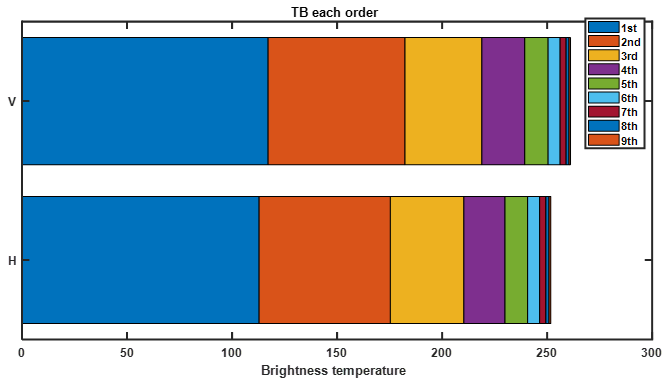
Figure A1 Contribution of brightness temperature from each order for 40°. The first several orders are shown for this simple case. In this particular case, contributions beyond the 2nd order have little contribution.

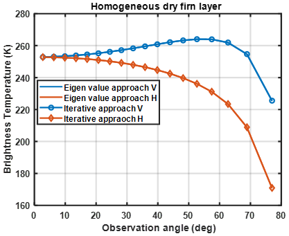
Figure A2 A single homogenous dry firn layer results from eigen value method and the iterative approach. The results from the two methods agree very well with each other.

Appendix B: Accumulation Radar echogram near FA-13

The accumulation radar echogram is provided in Fig. B1. This figure shows the water table locations along the flight track. The FA-13 site is on the left of the echogram.

Figure B1 Accumulation Radar data in 2014 near FA-13.

Appendix C: Temperature profile of FA-15

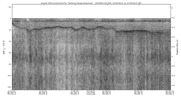
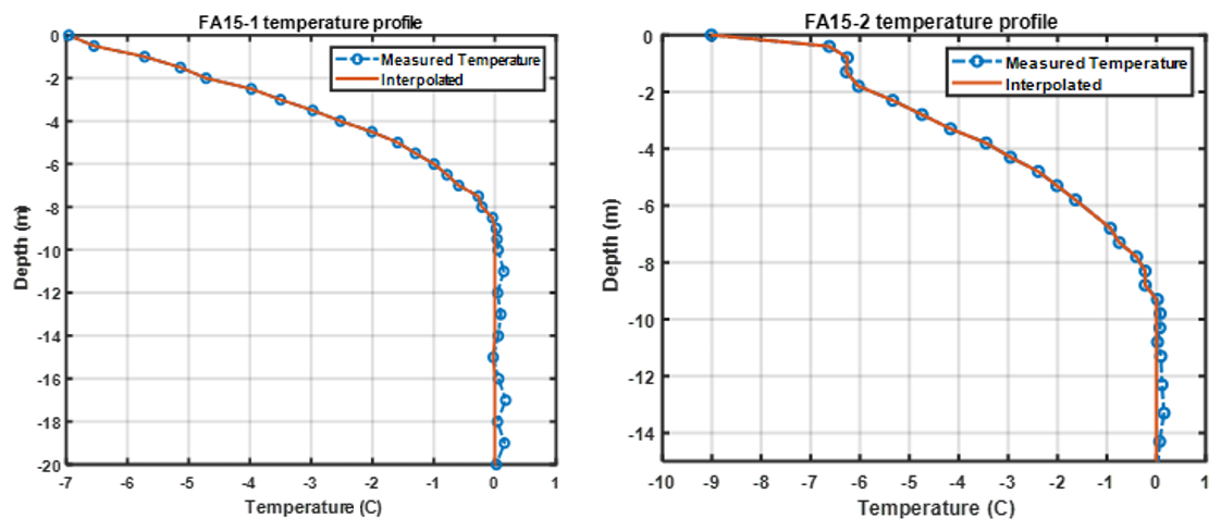
Figure C1 Temperature(left) of FA15-1 and FA15-2 (Miller et al., 2017). The water table locations are 19.8 and 14.4 m, respectively. Unlike what is observed in FA-13, where the physical temperature becomes 0° C at the interface of the dry firn and aquifer, the physical temperature profiles in these two boreholes reach 0° C before reaching the aquifer water table.