Investigating the impact of sub-ice shelf melt on Antarctic ice sheet spin-up and projections

Sub-ice shelf melting is critical for the stability of the Antarctic ice sheet, as it influences ice-shelf buttressing that reduces grounded ice flow. Previous studies have emphasized that uncertainties in the state of sub-ice shelf melting contribute to uncertainties in future sea-level projections. To better understand how sub-ice shelf melt rates affect model initialization and predictions, we adopt a single ice-sheet model (PISM) and investigate two different sub-ice shelf melt rate schemes during model spin-ups. We then drive the Antarctic ice sheet into the future using identical environmental forcings. We find that, despite closely matched steady-state geometries achieved through the spin-up process with different sub-ice shelf melt rates, the prognostic simulations reveal significantly divergent ice mass changes, particularly in marine ice sheet regions. By 2100, the difference in global sea-level contributions from the Antarctic ice sheet can be as large as ∼ 57 %, primarily from West Antarctica. This discrepancy arises because the spin-up initialization method alters the ice sheet's dynamic state, such as basal friction and thermal regimes, leading to differences in ice-sheet mass changes over time. Therefore, this study underscores the importance of sub-ice shelf melting and ice-sheet model initialization methods in reducing uncertainties in predicting the Antarctic ice sheet's future.

1 Introduction

A substantial majority of Antarctica's grounded ice discharges through its fringing ice shelves, which provide critical buttressing to upstream ice through two primary mechanisms: lateral shear stresses along sidewalls and basal resistance forces at pinning points on topographic highs (Schoof, 2007; Goldberg et al., 2009; Feldmann and Levermann, 2023; Feldmann et al., 2024; Miles and Bingham, 2024). Ice shelves are highly vulnerable to oceanic forcing due to the near-flotation elevation exposes them to warm seawater, which causes enhanced basal melting (Bindschadler et al., 2013; Depoorter et al., 2013; Li et al., 2023). Observations reveal accelerating ocean-driven thinning of Antarctic ice shelves over recent decades (Paolo et al., 2015; Rignot et al., 2019), where enhanced basal melting reduces buttressing effects and promotes grounding-line retreat, which collectively represent the primary driver of increased ice discharge (Jacobs et al., 2011; Pritchard et al., 2012; Seroussi et al., 2014; Jourdain et al., 2020; Reese et al., 2020). Particularly on retrograde bed slopes, such retreat may trigger Marine Ice Sheet Instability (MISI), a critical feedback mechanism that is often identified as a decisive factor in the collapse of the West Antarctica (Schoof, 2007; Hill et al., 2024). This process may amplify Antarctica's contribution to global sea-level rise by 0.5 to 0.8 m of sea-level equivalent (m SLE) this century (Ritz et al., 2015).

Methods for ice-sheet models to represent sub-ice shelf melting include linear/non-linear and local/non-local dependency thermal forcing parameterizations (Martin et al., 2011; Favier et al., 2019; Lowry et al., 2021), ice-shelf cavity models developed from box or plume models (Lazeroms et al., 2018; PICO, Reese et al., 2018; Favier et al., 2019; PICOP, Pelle et al., 2019), empirical approximations (Cornford et al., 2015, 2020), basin-averaged melt estimates (Seroussi et al., 2019), and spatially partitioned quadratic parameterizations (ISMIP6 protocol, Jourdain et al., 2020). The initMIP-Antarctica experiments revealed that ice-sheet model responses exhibit significant divergence due to variations in initial basal melting conditions, with the resulting range accounting for 5 % to 125 % of the total mass change (Seroussi et al., 2019, 2020). This pronounced model spread underscores persistent challenges in accurately representing sub-ice shelf oceanic processes during ice-sheet model initialization (Pritchard et al., 2012; Alevropoulos-Borrill et al., 2020), and may propagate into projection uncertainties, particularly for ice dynamics influenced by oceanic forcing. For instance, simulations with the Yelmo ice-sheet model indicate that the Antarctic ice sheet's sea-level contribution is highly sensitive to the ice-ocean interaction under varying basal melt coefficients, with several projections reaching up to 3 m SLE by 2500 (Juarez-Martínez et al., 2024).

Previous model intercomparison projects (e.g., initMIP-Antarctica; Seroussi et al., 2019) combined ice-sheet models with varying numerical complexities and initialization methods, making it difficult to attribute uncertainties to specific sources; our study isolates the impact of oceanic conditions by using a single ice-sheet model with identical initialization except for the basal melting scheme. Zhang et al. (2024) addressed this limitation by adopting a single ice-sheet model (Community Ice Sheet Model, CISM; Lipscomb et al., 2019; Berdahl et al., 2023) to investigate the impacts of geothermal heat flux and basal sliding conditions on Greenland Ice Sheet initialization. Extending this approach and considering the crucial role of ice shelves in Antarctica, we propose conducting similar experiments for the Antarctic ice sheet (AIS) using a single ice-sheet model and initialization method to assess the impacts of sub-ice shelf melt rates. This focused investigation will address two key questions: (1) How do varying sub-ice shelf melt rates impact the model initialization state? (2) How does this initial state affect long-term AIS projections?

Therefore, in this paper, we consider two different sub-ice shelf melt rates schemes (Sect. 2) in the Parallel Ice Sheet Model by first spinning-up and then projecting the AIS. The structure of this paper is organized as follows: Sect. 2 details the methodological approach and experimental design for spin-up and projection. Sections 3 and 4 provide comprehensive results and discuss the implications for ice dynamics and sea-level rise projections, while Sect. 5 analyses uncertainties in the model initialization and projection.

2 Model and Methods

We conduct ice-sheet simulations using the Parallel Ice Sheet Model (PISM v.1.0) (Bueler et al., 2007; Martin et al., 2011; Winkelmann et al., 2011; Albrecht et al., 2020), an open-source, three-dimensional thermomechanical coupled model that integrates ice dynamics and thermodynamics. The PISM employs a hybrid stress balance strategy (Martin et al., 2011; Winkelmann et al., 2011) by combining the Shallow Ice Approximation (SIA) for grounded ice (Gudmundsson, 2003; Bueler et al., 2007; Pollard and DeConto, 2012) and the Shallow Shelf Approximation (SSA) for floating ice (Hindmarsh, 2006; Bueler and Brown, 2009; Pollard and DeConto, 2012). In this ice-sheet model, basal resistance, which directly governs sliding velocities, is calculated using a generalized power law that ranges from plastic Coulomb sliding to linear sliding (Bueler and Brown, 2009; Winkelmann et al., 2011; Garbe et al., 2020). The grounding-line migration in PISM is determined through a sub-grid scheme, which interpolates key physical variables such as basal shear stress, basal melt rate, and basal friction based on spatial gradients across the interface between grounded and floating cells (Feldmann et al., 2014; Nowicki et al.,2020). This approach reduces physical gradients across the grounding line and simulates a more realistic and dynamic representation of the ice margin (Leguy et al., 2014; Golledge et al., 2015).

We utilize the BedMachine v.3 dataset (Morlighem et al., 2019) for initial topography, encompassing ice thickness and bedrock topography. Air temperature and precipitation inputs are derived from RACMO 2.3p2, averaged over 1979–2014 (van Wessem et al., 2018). Surface mass balance is calculated using a degree-day model (Ohmura, 2001; Calov and Greve, 2005), with near-surface temperature locally adjusted based on elevation changes using a correction factor of 0.008 °C m⁻¹ (Pittard et al., 2022). The PISM ocean module supplies the ice dynamics core with sub-ice shelf temperature and mass flux, with the former applied as a Dirichlet boundary condition in the energy conservation code, and the latter as a source in the mass conservation equation (Martin et al., 2011).

For model spin-up, where directly using observed basal melt rates (Rignot et al., 2013; Fig. 1), which are derived from satellite altimetry (ICESat-1), radar (OIB/ALOS PALSAR), and regional climate outputs (RACMO2), and ice-shelf basal temperature (Chambers et al., 2021; Fig. 1), the sub-ice shelf mass flux is given by:

$$\begin{array}{}\text{(1)}& S_{\mathrm{1}}={\mathit{\rho }}_{\mathrm{i}}B\end{array}$$

where ρ_i indicates the ice density, and B represents the sub-ice shelf melt rates. For simulations driven by Southern Ocean temperature and salinity (Schmidtko et al., 2014; Fig. 2) as implemented in LOW21 (Lowry et al., 2021), the mass flux at ice-ocean interface – representing the coupled melting effect of ocean temperature and salinity – is obtained indirectly through a simplified linear thermal forcing (TF-linear) parameterization (Beckmann and Goosse, 2003; Martin et al., 2011):

$$\begin{array}{}\text{(2)}& S_{\mathrm{2}}={\mathit{\rho }}_{\mathrm{sw}}{c}_{\mathrm{m}}{\mathit{\gamma }}_{\mathrm{T}}{F}_{\mathrm{melt}}\left(T_{\mathrm{s}}-T_{\mathrm{f}}\right)/\left(L_{\mathrm{i}}{\mathit{\rho }}_{\mathrm{i}}\right),\end{array}$$

where ρ_sw denotes the seawater density, c_m represents the specific heat capacity of the ocean mixed layer, L_i refers to the latent heat of phase change for ice, γ_T represents the thermal exchange velocity between seawater and ice (assigned ${\mathit{\gamma }}_{\mathrm{T}}={\mathrm{10}}^{-\mathrm{4}}$; Hellmer and Olbers, 1989; Holland and Jenkins, 1999), F_melt is a model parameter (assigned $F_{\mathrm{melt}}=\mathrm{5}\times {\mathrm{10}}^{-\mathrm{3}}$; Beckmann and Goosse, 2003). T_s is the vertically averaged ocean temperature between 200 and 1000 m depth along the continental slope, representing relatively warm water masses of the coastal current (Holland and Jenkins, 1999; Beckmann and Goosse, 2003). T_f denotes the freezing temperature of seawater:

$$\begin{array}{}\text{(3)}& T_{\mathrm{f}}=\mathrm{273.15}+\mathrm{0.0939}-\mathrm{0.057}{S}_{\mathrm{0}}+\mathrm{7.64}\times {\mathrm{10}}^{-\mathrm{4}}{z}_{\mathrm{b}}\end{array}$$

where S₀ denotes the specified ocean salinity, z_b as the elevation (generally negative) of the base of the ice shelf.

We applied a “multi-stage” spin-up procedure (Golledge et al., 2015; Lowry et al., 2021) to achieve a pseudo-equilibrium ice-sheet state under constant climate conditions, with a 16 km spatial resolution: (1) a brief 10-year smoothing utilizing the shallow ice approximation, (2) a 250 000-year thermal evolution run with the “no_mass” option, which fixes the ice geometry and allows the enthalpy field to evolve to equilibrium, (3) a 1500-year model run incorporating full model physics, including the application of sub-ice shelf melt rates to constrain ice dynamics, and (4) a 65-year historical run to connect initialization and prediction, during which the current ice thickness is reconstructed.

In projection, to ensure that differences in results originated solely from the model spin-up, we employed the same daily-resolution climate forcings as LOW21 (Lowry et al., 2021), derived from the CMIP5 IPSL-CM5A-MR RCP 2.6/8.5 (2015–2100; Barthel et al., 2020; Payne et al., 2021; Nowicki et al., 2021). Furthermore, we also conducted the experiments to include SSP scenarios for Antarctic ice-sheet evolution, using daily climate forcings from the CMIP6 CNRM-CM6-1 SSP 1–2.6/5–8.5 product (Nowicki et al., 2016; Kamworapan et al., 2021; Nowicki et al., 2021) spanning 2015–2100. These daily data were pre-processed by averaging to produce annual mean forcings, which were then used to drive the ice-sheet model. The basal melting scheme was parameterized using the same linear thermodynamic framework (S2) for the ice-shelf-ocean boundary layer as that employed in LOW21 – specifically, the approach defined in Eq. (2), which is driven by the annual-mean spatial distribution and time series of absolute salinity and temperature fields derived from the RCP/SSP scenarios (Jourdain et al., 2020; Nowicki et al., 2020). We have conducted projection experiments from 2015 by turning on or off the sub-grid grounding-line scheme in PISM. The “sub-grid scheme on (SGO) scenario” incorporated sub-grid melt interpolation near grounding lines, accelerating their retreat in the coarse-resolution model, while the “sub-grid scheme off (SGF) scenario” ignored melt in partially floating cells, yielding more conservative mass loss estimates (Albrecht et al., 2011; Golledge et al., 2015; Nowicki et al.,2020).

In summary, with the above approach, we produced two sets of simulations that differ essentially only in their ice-sheet initial state (Fig. 3). During spin-up, “S1 simulations” were forced by the basal melting derived from Eq. (1), and “S2 simulations” were forced by basal melting obtained from Eq. (2). For the projections, both S1 and S2 simulations were forced using the same method – basal melting calculated from Eq. (2), driven by salinity and temperature from climate scenarios. For S1 simulations, projections were performed for both RCP and SSP scenarios, while S2 simulations, which were obtained from LOW21, were conducted only for the RCP scenarios. Although S1 simulations are initialized with the S1 method (Eq. 1), but driven by the S2 parameterization (Eq. 2) for projections, their results are not contaminated by a potential shock (Appendix A).

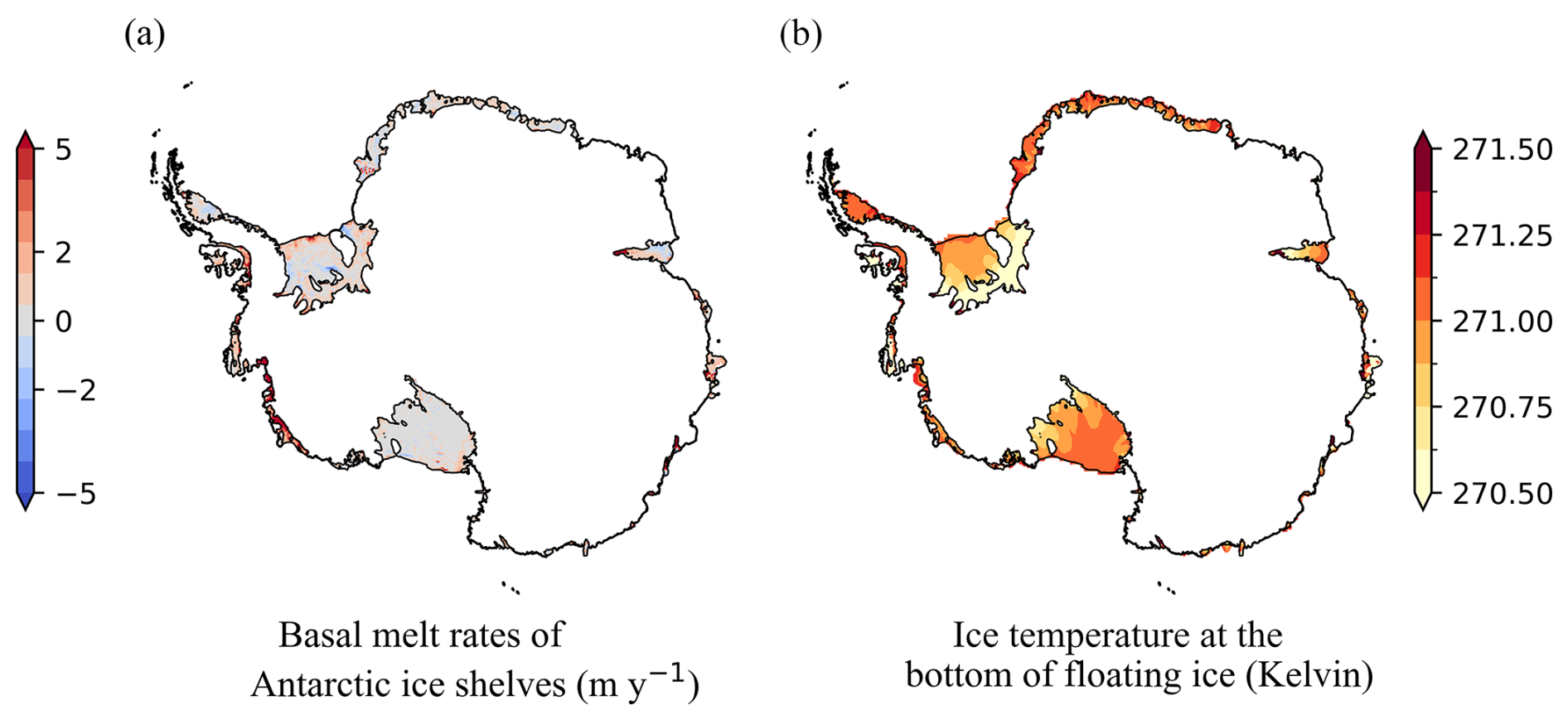
Figure 1 Ocean conditions used in S1 spin-up. (a) observation of sub-ice shelf basal melt rates (Rignot et al., 2013); (b) Temperature field beneath ice shelves (Chambers et al., 2021).

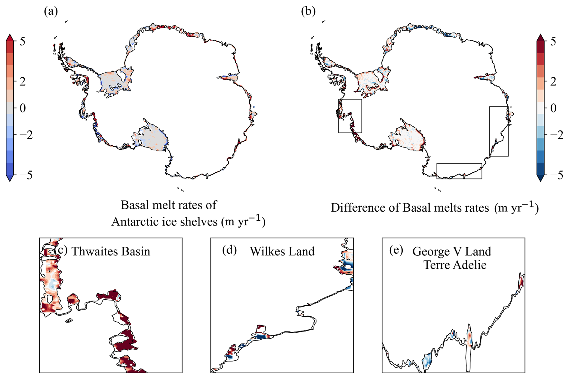
Figure 2 Comparison of initial sub-ice shelf melt rates between S1 and S2 spin-ups. (a) Sub-ice shelf melt rates derived from the TF-linear parameterization (S2). (b) Difference in basal melt rates (S1–S2). Regions of interest are highlighted by black boxes: (c) Thwaites Basin, (d) Wilkes Land, and (e) George V Land–Terre Adelie.

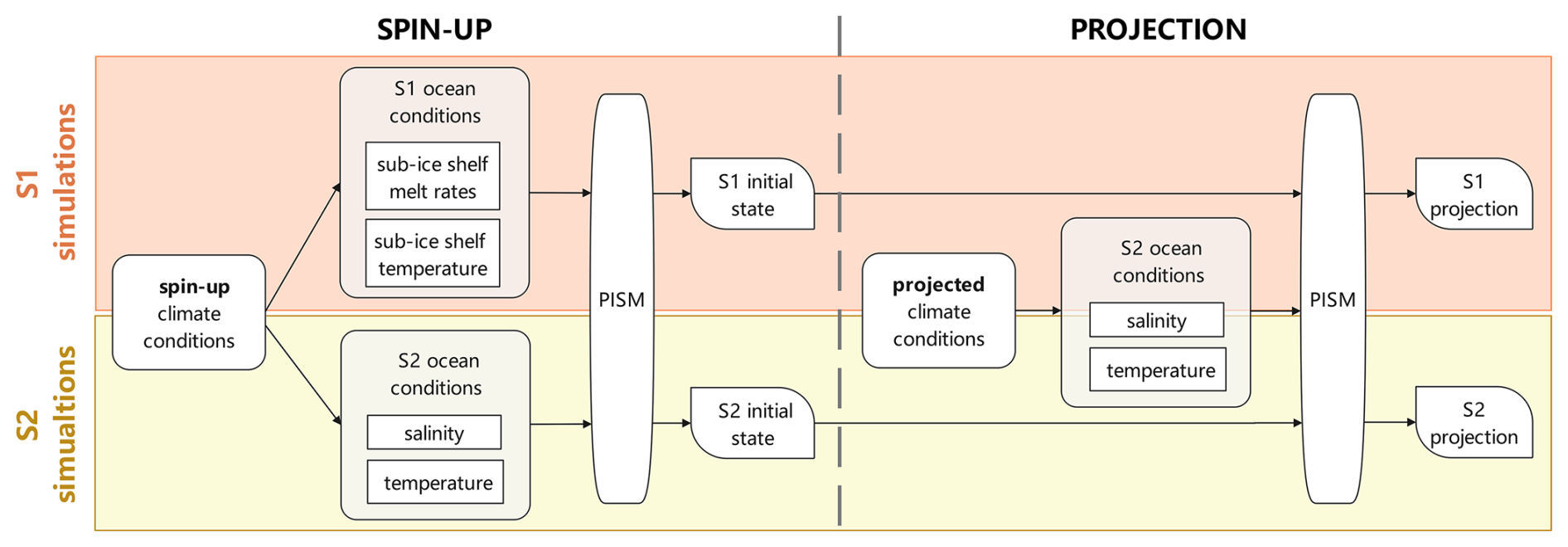
Figure 3 Overview of model spin-up and projection processes. The schematic summarizes the model setup during spin-up and projection. The ocean initialization employs two distinct schemes: using observed basal melt rates along with ice-shelf basal temperature (S1 simulations, orange box), and using Southern Ocean temperature and salinity (S2 simulations, yellow box; reproducing LOW21). Projections initialized from these two ice-sheet states and forced with an identical basal melting method (Eq. 2) as well as future oceanic conditions from 2015 to 2100.

3 Model Initialization Results

3.1 Comparison with the case of different sub-ice shelf melt rates

We validated the simulated ice-sheet geometry from both S1 and S2 using observational datasets (BedMachine v.3; MEaSUREs Phase-Based Antarctica Ice Velocity Map v.1). The results show that both simulations achieve comparable accuracy against observations: the root mean square errors (RMSE) for ice thickness are approximately 89 m (S1) and 87 m (S2), differing by 2 m; the RMSE for ice surface velocity are roughly 270 m yr⁻¹ (S1) and 267 m yr⁻¹ (S2), differing by 3 m yr⁻¹. The comparison (Fig. 4) shows that the ice-mass distribution and ice flow of S1 also closely match those of S2. To better highlight regions with notable discrepancies in ice thickness and ice surface velocity between the two simulations, such as Thwaites Glacier, we selected a representative transect to compare the grounding-line positions, ice thickness, and surface velocity profiles between S1 and S2.

We also compared the results of two simulations against those from the Antarctic ice-sheet model initialization (initMIP-Antarctica) that employed PISM (Seroussi et al., 2019). Both studies align with ensemble trends in ice mass, ice sheet area, ice shelf area, and potential sea-level contributions. S1 simulations exhibit minor differences in total ice sheet mass (−6 % to +11 %) and ice area (−7 % to −1 %) compared to initMIP-Antarctica. Notably, deviations in potential sea-level contributions are more pronounced (−17 % to −2 %), while ice shelf area discrepancies reach 44 % relative to the DMI_PISM simulation (Fig. 5). Overall, despite minor differences in other metrics between two simulations and the initMIP-Antarctica ensemble simulations, the spin-up ice volumes (potential sea-level contributions) in both S1 (25.81 × 10⁶ km³) and S2 (25.77 × 10⁶ km³) exhibit close agreement with the observed total ice volume (BedMachine v.3; 26 (± 0.4) × 10⁶ km³). This validates the robustness of our initialization configuration and gives confidence for future projection experiments.

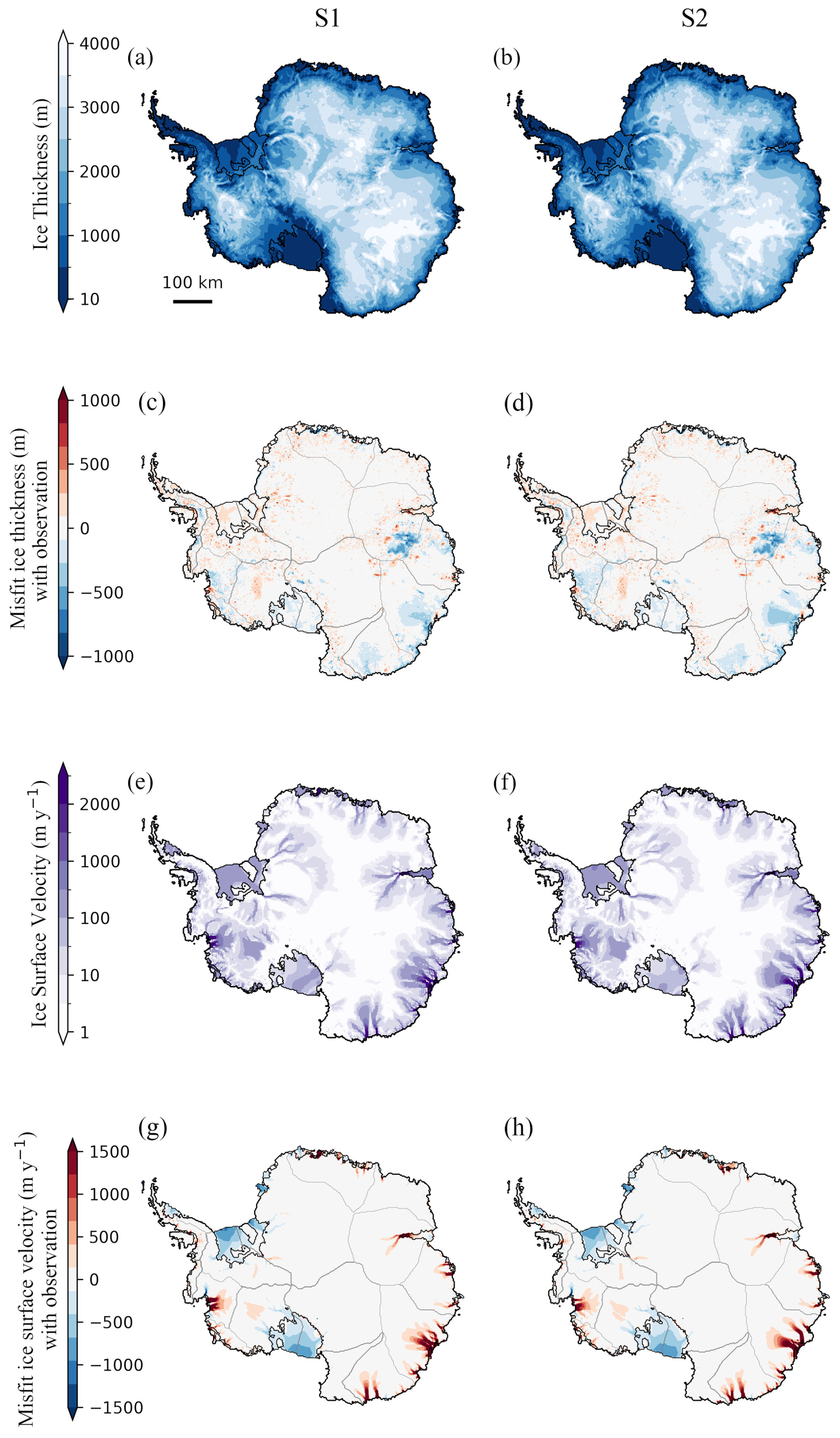
Figure 4 Comparing simulated initial state with observations. Modeled ice thickness (m) and ice surface velocity (m yr⁻¹) at the end of spin-up. The left column shows ice thickness and ice surface velocity results from S1, alongside their misfits from observation (Morlighem et al., 2019; Mouginot et al., 2019). The right column shows the corresponding results from S2, sharing common color bars with S1.

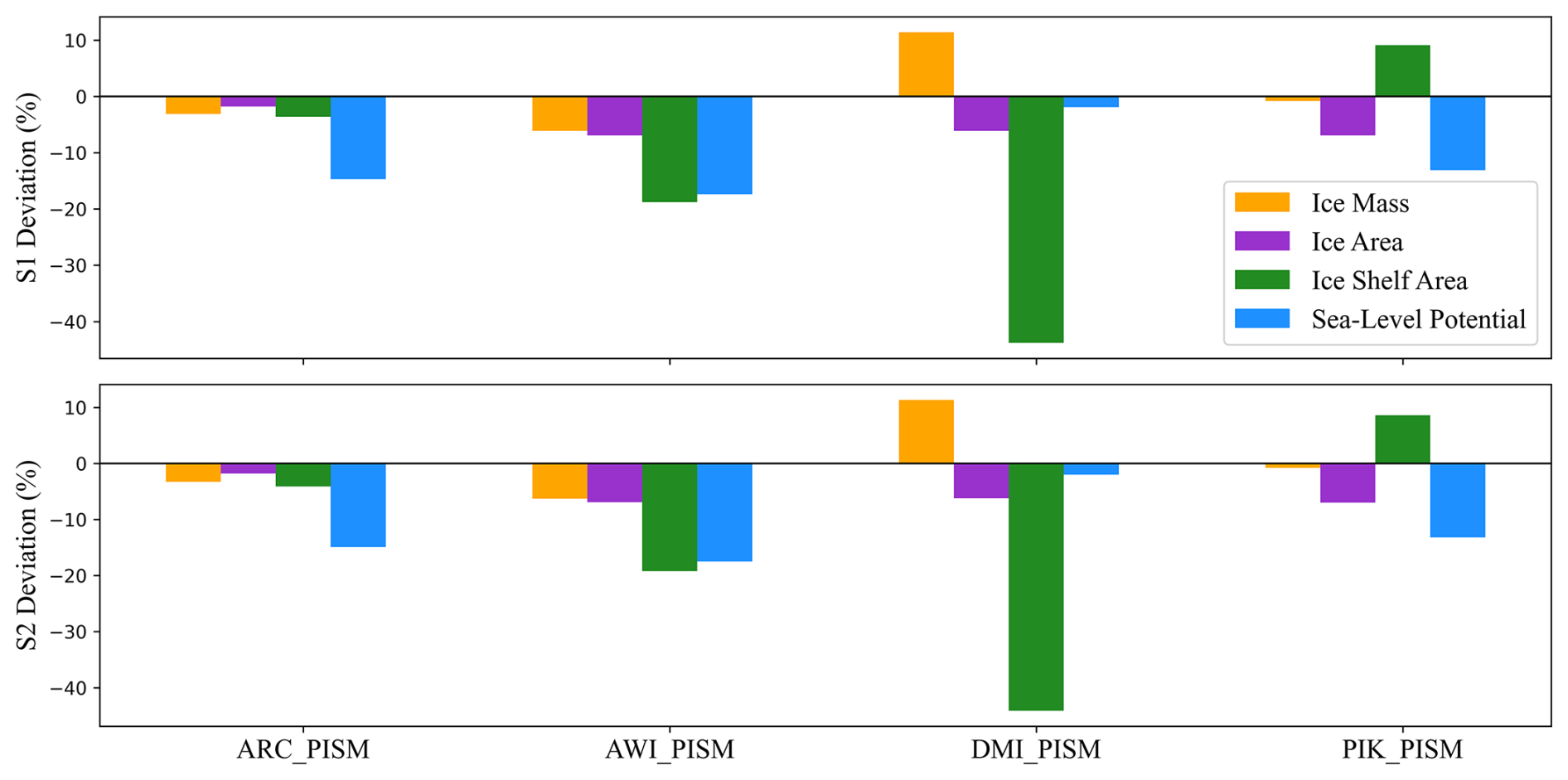
Figure 5 Percentage deviations in steady-state metrics (ice mass, ice sheet area, ice shelf area, potential sea-level contribution) relative to the initMIP-Antarctica PISM-based ensemble. The vertical axis represents the percentage deviation between the results of S1, S2, and the simulations from participating institutions (^*_PISM, where ^* denotes the institution abbreviation).

3.2 Differences in Marine Ice-sheet regions

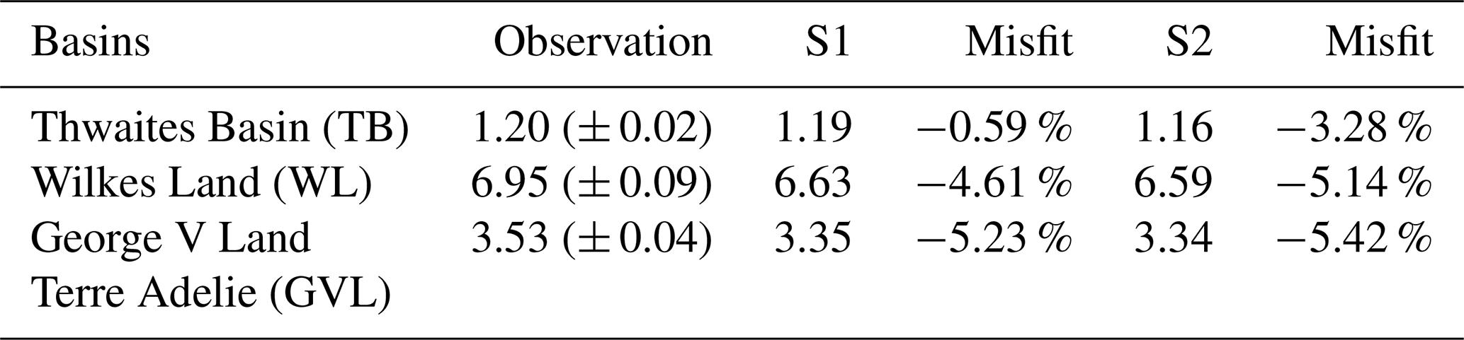
There are significant ice surface velocity differences in three marine-based regions characterized by retrograde bed slopes (Fig. 6): Thwaites Basin (TB) in the West Antarctica (WAIS), Wilkes Land (WL), and George V Land–Terre Adelie (GVL) in the East Antarctica (EAIS). These regions are particularly susceptible to MISI due to their subglacial topography (Joughin et al., 2014; Mengel and Levermann, 2014; Greenbaum et al., 2015).

In the Thwaites Basin, the observed sub-ice shelf melt rates used in S1 (reaching 17.7 m yr⁻¹ beneath Thwaites ice shelf; Fig. 1) exceed S2's parameterized values by approximately 5 m yr⁻¹ (Fig. 2). This higher basal melting weakens the ice-shelf buttressing effect and accelerates the grounded ice flow, with a corresponding 74 m yr⁻¹ RMSE difference from S2 (RMSE_S1–RMSE_S2; Fig. 6f). Compared to S2, this results in around 40 m more ice thinning near the grounding line and an approximately 30 km more grounding-line retreat (Fig. 8), demonstrating an intrinsic connection within the ice-sheet system. This systemic response is further evidenced by widespread thickening upstream, with a mean anomaly of 49.5 m. The ice volume above flotation in S1 shows a 5.5-fold bias reduction (−0.59 %; 1.19 m SLE) compared to S2 (−3.28 %; 1.16 m SLE), aligning closely with observations (1.20 ± 0.02 m SLE; Table 1).

In the Wilkes Land, the Totten Glacier exhibits increased ice flow under observed melt rates, yielding a 44 m yr⁻¹ lower RMSE in S1 relative to S2 (RMSE_S1–RMSE_S2; Fig. 6g), leading to regional mean ice thinning of 38.5 m. The faster flow of Totten Glacier strengthens lateral resistance along its boundaries with adjacent glaciers, subsequently reducing ice flux into the Voyeykov and Moscow Ice Shelves (Gagliardini et al., 2010; Van Der Veen et al., 2014). This dynamic response is consistent with the simulated mean thickness anomaly of +39.2 m across these regions. The ice volume above flotation bias in WL decreases to −4.61 % (6.63 m SLE) in S1, compared to −5.14 % (6.59 m SLE) in S2, achieving a 10 % improvement relative to the observed 6.95 ± 0.09 m SLE (Table 1).

In the George V Land–Terre Adelie, the enhanced flow of the Ninnis Ice Shelf in S1 results in increased ice discharge and regional mean thinning (33.7 m; Fig. 6c). Conversely, the Cook and Mertz Ice Shelves and their upstream glaciers experience reduced ice flux, causing regional ice thickness to increase by 25.5 m on average relative to S2. S1 simulations demonstrate a reduced ice volume above flotation bias of −5.23 % (3.35 m SLE) in WL, outperforming −5.42 % (3.34 m SLE) of S2 and reflecting closer agreement with the observed 3.53 ± 0.04 m SLE (Table 1).

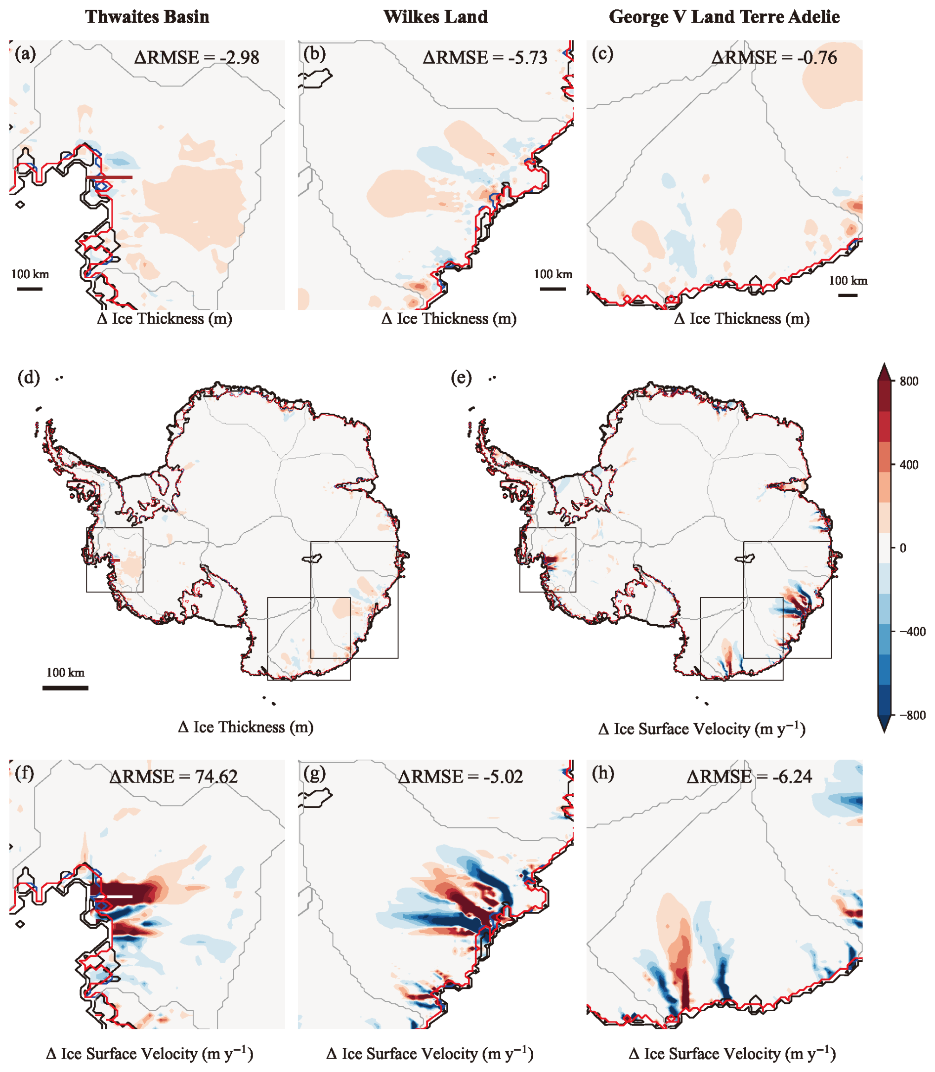
Figure 6 Comparison of spin-up ice thickness and ice surface velocity differences between S1 and S2. (a–c) Ice thickness differences (S1–S2) in the TB, WL, and GVL, respectively. (f–h) Ice surface velocity differences (S1–S2) in the TB, WL, and GVL, respectively. The difference in root mean square error between S1 and S2 (ΔRMSE = RMSE_S1–RMSE_S2), compared to observations. (d) and (e) present the deviations in ice thickness and ice surface velocity between two simulations, with three black boxes highlighting regions showing the most significant discrepancies. Grounding lines: S1 (red), S2 (blue), and observed data (black) from BedMachine v.3 (Morlighem et al., 2019). The profile line locations corresponding to Fig. 8 are in Thwaites Glacier: (a), (d) brown; (f) white.

A comparison of simulation results for ice volume above flotation between S1 and S2 across three marine ice sheet basins (TB, WL, and GVL; Table 1) reveals that the ice-sheet model driven by observed sub-ice shelf melt rates achieves slightly better alignment with observations. Although the RMSE of ice surface velocity in the TB shows an increase of 74 m yr⁻¹ in S1 compared to S2 (RMSE_S1–RMSE_S2; Fig. 6f), the bias in ice volume above flotation decreases by approximately 2.8 %, while the biases for WL and GVL are reduced by 0.5 % and 0.2 % (Misfit_S1–Misfit_S2; Table 1), respectively.

Table 1 Ice volume above flotation (m SLE) in three marine ice sheet basins after spin-up, simulated at 16 km resolution. Misfit (in %) denotes the percentage deviation of the S1 and S2 simulation results from observations, respectively.

3.3 Marine Ice Sheet dynamics during model spin-up

In the WAIS, particularly for glaciers adjacent to the Amundsen Sea Embayment, the subglacial bedrock topography lying below sea level amplifies the sensitivity to ocean-driven forcings (Pritchard et al., 2012). Previous studies stated that the Aurora Subglacial Basin in WL and the Wilkes Subglacial Basin in GVL, in the EAIS, are characterized by extensive sedimentary basins that are highly susceptible to warming ocean conditions (Aitken et al., 2014; Frederick et al., 2016; Noble et al., 2020). These basins are also subject to an active subglacial hydrology process (Wright et al., 2012), and evidence of ocean-driven dynamic ice loss has been documented along the ice-sheet margin (Li et al., 2016). The interplay between oceanic forcing, subglacial hydrology, and sedimentary geology significantly influences ice-sheet dynamics in these regions.

In the S1 simulations, enhanced oceanic forcing (Fig. 2), which is represented by higher basal melt rates, intensifies ice-shelf basal melting, leading to geometric thinning and reduced buttressing effect of upstream ice flow (Gudmundsson, 2013; Miles et al., 2022). This triggers grounding-line retreat, which accelerates ice flow, amplifies strain rates, and enhances dissipative heating (Cuffey and Paterson, 2010; Dawson et al., 2022), thereby increasing temperatures at the basal ice layer (Fig. 7a–c). It then promotes basal melting (Fig. 7d–f) while reducing ice viscosity via thermal softening, collectively facilitating enhanced deformation and potentially increasing ice-sheet destabilization (Hindmarsh, 2006; Adams et al., 2021). Additionally, subglacial meltwater lubricates the ice-bedrock interface, reducing basal friction through decreased effective pressure and accelerating ice flow (Fig. 7g–l). Enhanced sliding generates additional strain heating (Garbe et al., 2020), which promotes further basal melting and meltwater production. In this positive feedback process, termed the basal thermal-hydrological feedback, elevated basal water content persistently reduces resistance, thereby facilitating ice sliding and ultimately leading to ice thinning (Fowler et al., 2001; Clarke, 2005; Van Pelt and Oleremans, 2012; Zhao et al., 2025).

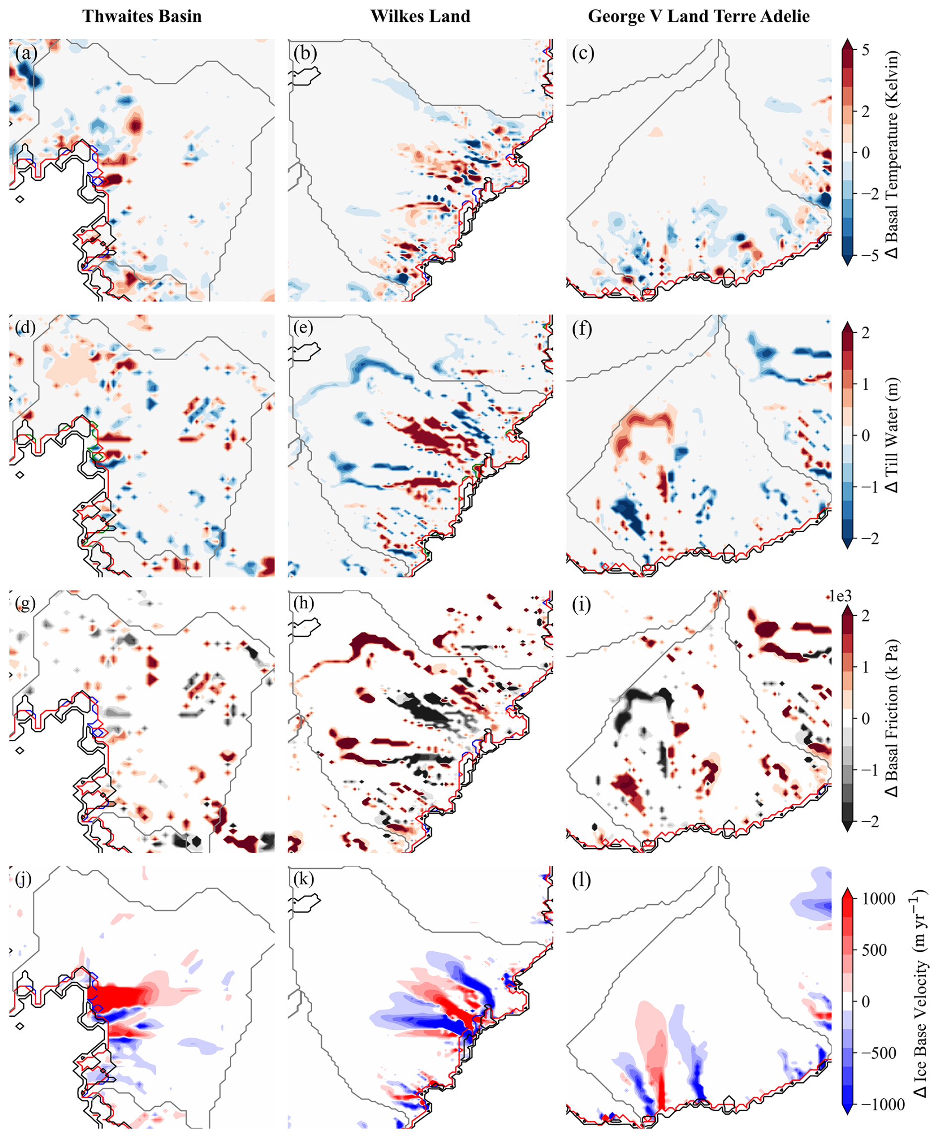
Figure 7 Spatial distribution of differences (S1–S2) in basal ice temperature field (Kelvin) (a–c), basal till water content (m) (d–f), basal friction (k Pa) (g–i), and basal ice velocity (m yr⁻¹) (j–l) in the three basins. The red and blue lines indicate the grounding-line positions for S1 and S2, respectively, while the black line represents the observed grounding line from BedMachine v.3.

3.4 Grounding line location comparison

The impact of sub-ice shelf melt rates on ice-sheet initialization is also apparent in the positions of the grounding line. In the WAIS, the retrograde bed topography amplifies the susceptibility to MISI (Pritchard et al., 2012; Ritz et al., 2015), rendering it highly responsive to ocean forcing. During spin-up, these elevated basal melt rates (Fig. 2) trigger MISI more easily, causing the grounding line on retrograde bedrock to retreat continuously until reaching a new steady state (Rignot et al., 2019; Li et al., 2022). Cross-sectional analysis of Thwaites Glacier (Fig. 8) demonstrates this mechanism, with enhanced basal melting, causing an approximately 30 km grounding-line retreat from a stabilized position (S2; dashed grey line) to a new quasi-stable state (S1; solid grey line). The retreat in S1 increases ice discharge due to the reduced ice-shelf buttressing effect, resulting in roughly 40 m ice thinning proximal to the grounding line and an anomalous nearly twofold acceleration in ice surface velocity compared to S2 results (S1–S2). This feedback highlights how ocean-forced basal melting propagates through ice-sheet dynamics processes to alter initial ice geometry.

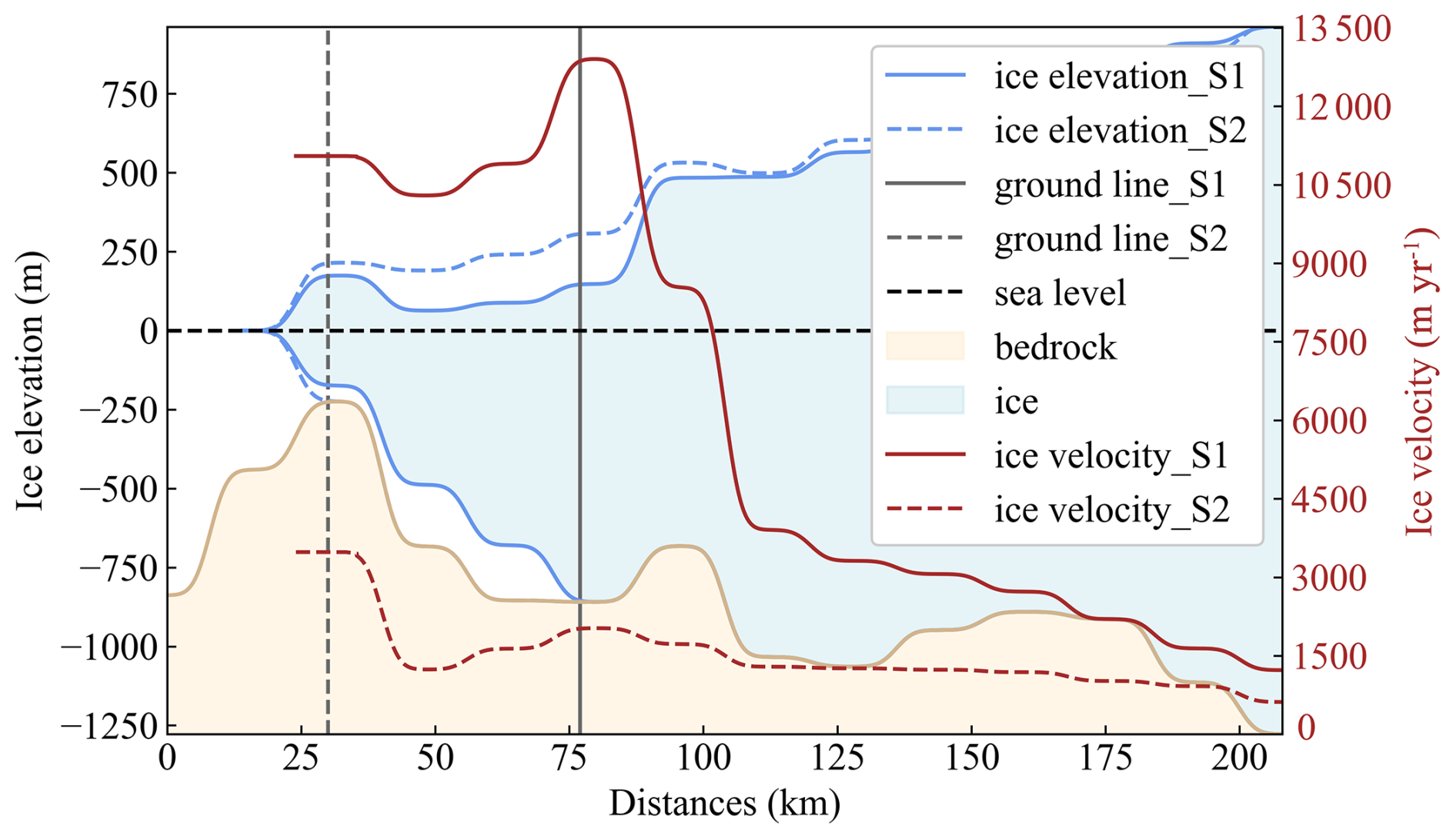
Figure 8 Comparison between S1 and S2 along the Thwaites Basin transect after spin-up. Ice elevation (blue line), ice surface velocity (brown line), and grounding-line positions for S1 and S2 are indicated by the grey solid and dashed lines, respectively. Sea level: black dashed line.

In fact, the grounding-line position varies across different ice streams depending on topography, neighbouring ice shelf basal melt rates, and ice velocities (Martin et al., 2011; Pittard et al., 2022), resulting in spatial discrepancies between observed and simulated grounding-line positions that vary spatially across the AIS. For instance, the grounding line of the Siple Coast on the west side of the Ross Ice Shelf in S1 agrees with S2 but extends further to the nearshore compared to the observation (Fig. 6d–e). This discrepancy likely arises from a self-limiting, stabilizing mechanism inherent to prograde slopes. As the grounding-line retreats into shallower bedrock, the ice thins and ice flux decreases; this leads to ice re-accumulation that prompts grounding-line readvancement, creating reversible shifts around an equilibrium point (Huybers et al., 2017). Notably, under a consistent model parameter configuration, the inclusion of observed sub-ice shelf melt rates did not significantly alter the steady-state grounding-line migration position across the whole AIS, except within three marine-based regions.

4 Model Projection Results

4.1 Global mean sea-level contribution from AIS

Prognostic simulations (2015–2100) show that the divergent initial ice-sheet states of S1 and S2 lead to markedly different sea-level contributions across the AIS, even under identical climatic forcings and basal melting scheme (Figs. 9 and 10). Specifically, S1 projected a 0.20–0.52 m SLE contribution from the AIS exceed the LOW21 ensemble projections (0–0.32 SLE; which includes predicted results from S2) by roughly 0.18 m SLE, representing a ∼ 57 % increase (Fig. 9). This discrepancy is driven primarily by enhanced ice loss from the West Antarctica (0.29–0.34 m SLE; Table 2), where high sub-ice shelf melt rates triggered MISI more readily, whereas the East Antarctica and the Antarctic Peninsula (AP) show minimal sea-level contributions by 2100, i.e., 0.01–0.02 m SLE and 0.0011–0.0045 m SLE, respectively (Table 2). However, the S1 projections from 2015–2075 exhibit no significant dependence on emission scenarios, with substantial overlap in prediction ranges (Fig. 9c). This is consistent with the hysteretic response of ice-sheet dynamics, meaning that the ice sheet's state in the near-term (2015–2075) is largely determined by historical forcing, masking the influence of divergent future scenarios (Garbe et al., 2020). By 2100, the mean AIS contributions to sea-level rise in S1 projections under SSP 5–8.5 reach 0.36 m SLE – 12.5 % higher than the RCP 8.5 equivalent (0.32 m SLE) – with RCP high-emission projections even matching SSP low-scenario results (Fig. 9d; Table 2). These differences between RCP 8.5 and SSP 5–8.5 projections are largely due to the SSP scenarios in CMIP6 climate models simulating higher warming magnitudes (averaging +0.14–0.25°) than RCP scenarios in CMIP5 at equivalent radiative forcing (Tokarska et al., 2020; Wyser et al., 2020; Rounce et al., 2023). Consequently, under anthropogenic warming, the sea-level commitment of AIS under SSP high-risk scenarios demands heightened scientific attention.

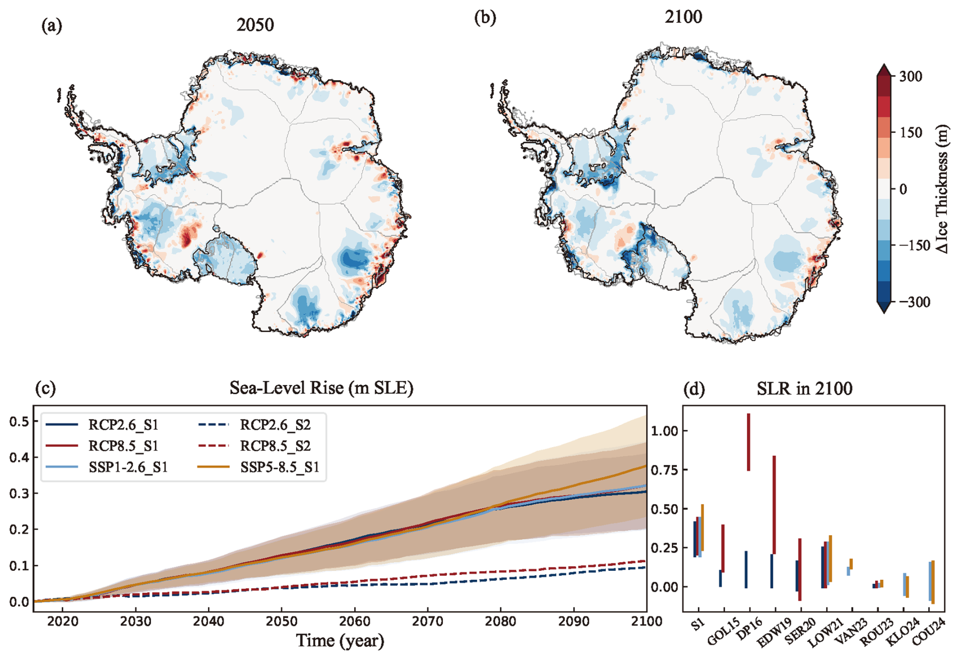
Figure 9 Ice sheet thickness differences and projected contributions of the AIS to sea-level rise (m SLE). Spatial differences in the projected ice thickness between the S1 and S2 multi-scenario ensemble means for 2050 (a) and 2100 (b). The values are derived by averaging the differences (S1–S2) under the RCP 2.6 (RCP 2.6_S1, RCP 2.6_S2) and RCP 8.5 (RCP 8.5_S1, RCP 8.5_S2) scenarios in (c). (c) Predicted sea-level rise for “SGO scenario” to “SGF scenario” simulations in S1 under four scenarios (color shading) and mean values (color lines). The dashed lines represent projections from the S2 initial state – a set of results from the LOW21 ensemble projections: red for RCP 8.5, blue for RCP 2.6. (d) Projected contributions to sea-level rise (SLR) by 2100 from the S1 simulations, compared to other studies: CHU13 (Church et al., 2013), GOL15 (Golledge et al., 2015), DP16 (DeConto and Pollard, 2016), EDW19 (Edwards et al., 2019), SER20 (Seroussi et al., 2020), LOW21 (Lowry et al., 2021), VAN23 (van der Linden et al., 2023), KLO24 (Klose et al., 2024), and COU24 (Coulon et al., 2024).

4.2 Regional Contributions to Global Mean Sea-Level Rise

To explore the spatially variable response of the AIS, we partitioned the ice sheet into seven sectors based on their adjacency to surrounding oceans (Fig. 10). This regional breakdown reveals stark contrasts in the mechanisms and magnitudes of sea-level rise across the WAIS, EAIS, and AP (Fig. 10; Table 2), highlighting their distinct sensitivities to climate forcings. The WAIS emerges as the primary driver of AIS-related sea-level rise, contributing 0.29–0.34 m SLE by 2100. A mechanism similar to that observed in recent decades may be responsible for the projected mass loss. Specifically, anthropogenic warming could alter shelf-break wind patterns over the Amundsen and Bellingshausen Sea (AS/BS) embayments (Holland et al., 2019; Noble et al., 2020), potentially facilitating greater intrusion of warm water and intensifying ice melting beneath ice shelves (Dinniman et al., 2016; Noble et al., 2020; Li et al., 2023). The resulting reduction in ice-shelf buttressing accelerates ice discharge, which explains the dominance of the AS and BS sectors – accounting for ∼ 55 % of total WAIS mass loss in S1 projections (Table 2).

Following the IMBIE (Zwally et al., 2012), we further subdivided the East Antarctica into the East Indian Ocean (EIO) and West Indian Ocean (WIO) sectors. The EAIS presents a more complex picture, with a net contribution of 0.01–0.02 m SLE by 2100; although the integrated signal is small, it masks pronounced regional heterogeneity in mass changes. The net mass gain in the WIO sector shown in the S1 projections may be linked to enhanced moisture transport from the Southern Ocean, a mechanism consistent with observational trends (Boening et al., 2012) that would promote increased ice surface accumulation. However, this marginal gain is counteracted by ice dynamical adjustments within the EIO sector, specifically across the WL, where enhanced oceanic thermal forcing drives accelerated ice mass loss from the dynamically vulnerable Totten Glacier (Konrad et al., 2018). This contrast between surface mass gains and ice-dynamic losses underscores the spatially heterogeneous response of EAIS, modulated by regional bathymetry and ocean-driven melt.

The AP plays a comparatively minor role in sea-level rise, with contributions ranging from 0.0011–0.0043 m SLE by 2100. Peak mass loss occurs between 2075 and 2079, reaching 0.0061 m SLE under RCP 8.5 and 0.0045 m SLE under SSP 5–8.5, followed by a gradual decline (Fig. 10). The intensification of polar westerly winds could enhanced snowfall in the northern AP, which may partially offset warming-induced ice discharge and thus generate a negative feedback that suppresses mass loss (Goodwin et al., 2016). Given its limited ice volume, however, the AP's overall impact on sea-level rise remains marginal. The findings underscore the divergent climate responses of the EAIS, AP, and the WAIS. While the EAIS and AP exhibit mass gain or loss depending on the balance between accumulation and ablation, the WAIS is primarily driven by dynamic mass loss resulting from changes in oceanographic conditions.

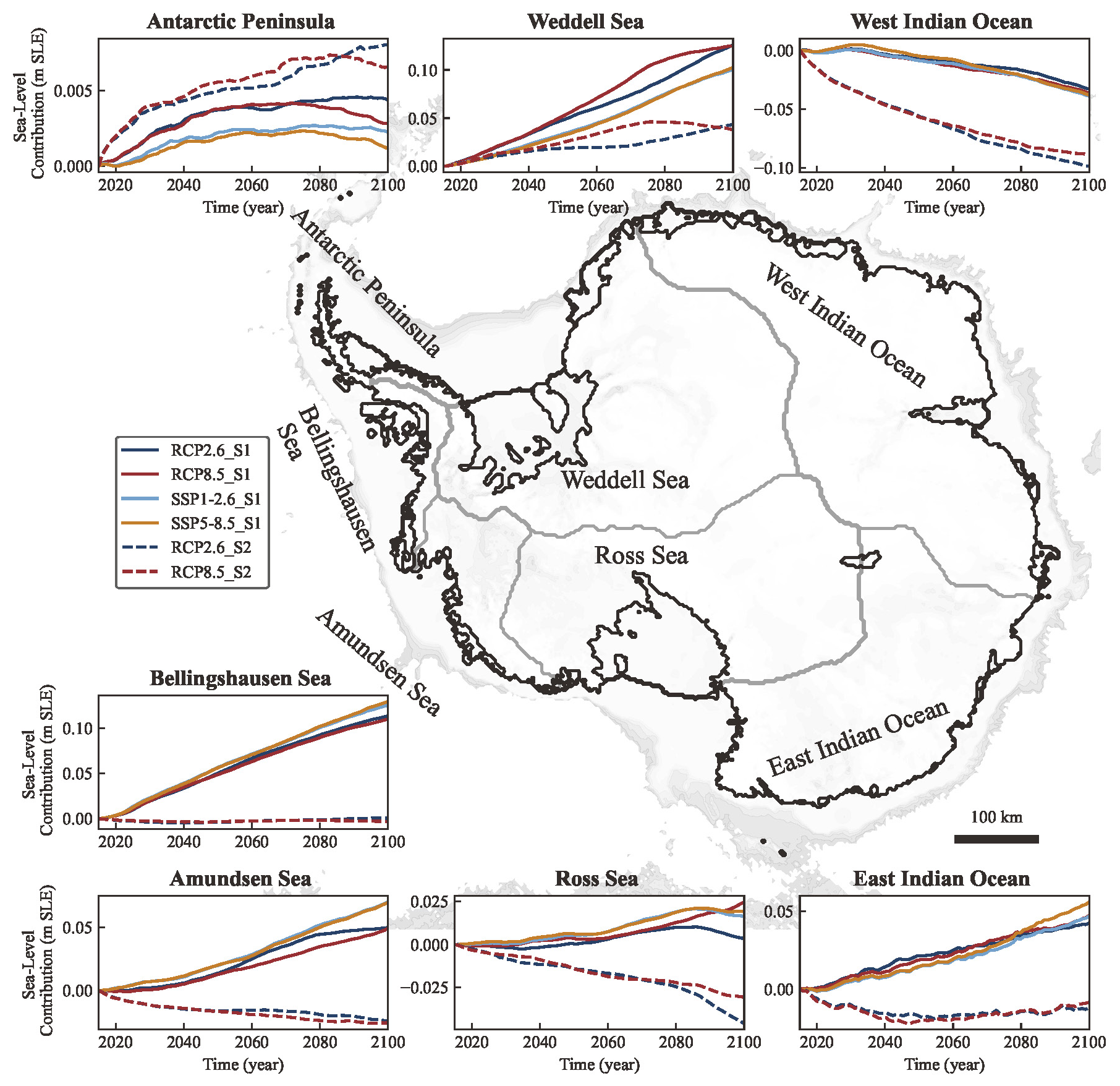
Figure 10 The mean contribution of the AIS seven sectors to sea-level rise from 2015 to 2100 (m SLE). The solid and dashed lines represent projections from the S1 and S2 initial states, respectively, under different climate scenarios, with the S2 predicted results being part of the LOW21 ensemble projections (red for RCP 8.5, blue for RCP 2.6).

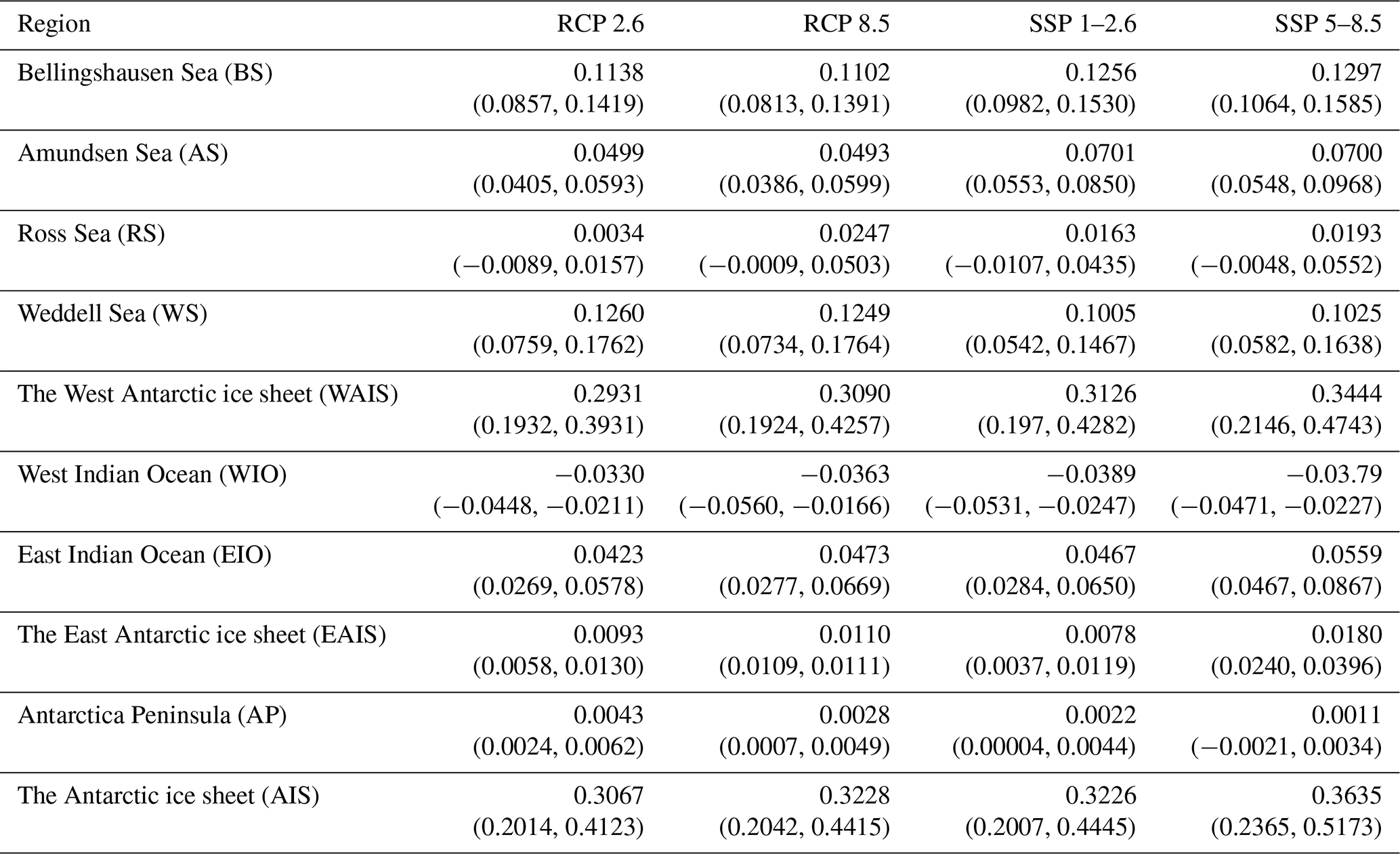
Table 2 Sea-level contribution (m SLE) of Antarctic ice sheet Basins by 2100 in S1 projections. The confidence intervals represent the range of sea-level contribution from the “SGO scenario” to the “SGF scenario” simulation across different RCP/SSP scenarios; the single value denotes the mean value of this range.

4.3 Comparison with previous projections

The S1 projections to sea-level rise by 2100 under the SSP 5–8.5 scenario diverge significantly from previous estimates, particularly for the WAIS. The Coupled Model Intercomparison Project Phase 6 models (CMIP6; Edwards et al., 2021) employed Gaussian process emulators – statistical approximations built upon ice-sheet simulations for ISMIP6 (Nowicki et al., 2016, 2020) and GlacierMIP Phase 2 (Hock et al., 2019) – to generate sea-level contributions. While their ensemble projections suggest that the WAIS contributions range from −0.04 to 0.11 m SLE, S1 projections show a significantly higher contribution of 0.20–0.47 m SLE. For the EAIS and AP, S1 projected sea-level contributions (0.03–0.04 m SLE and −0.0021–0.0034 m SLE, respectively; Table 2) align closely with the emulator results (−0.05–0.06 m SLE and −0.01–0.02 m SLE, respectively), with the WAIS emerging as the dominant divergence source.

Compared to the full ensemble results of ISMIP6 (Ice Sheet Model Intercomparison for CMIP6) Antarctic projections under RCP 8.5 (Seroussi et al., 2020), the S1 projected sea-level contributions for the WAIS are approximately 0.15 m SLE higher, while the AP shows a slight increase (∼ 0.002 m SLE), and the EAIS exhibits a minor reduction (∼ 0.02 m SLE). The ISMIP6-Antarctica projections provide a more comprehensive representation of potential Antarctic sea-level contribution under climatic forcings, with the parameterizations of oceanic conditions into basal melt rates being the dominant source of uncertainty (Seroussi et al., 2020). However, these experiments cannot identify the specific physical mechanisms behind the inter-model differences. Although a key limitation of our single model experiments is its reliance on PISM-specific parameterizations, which restrict the range of projected sea-level contributions and provide limited statistical uncertainty. Nevertheless, by comparing observed and parameterized basal melt rates as represented in model simulations under a consistent single-model framework, our results identify the specific regions and dynamic mechanisms underlying the ISMIP6 projection uncertainty associated with the representation of oceanic conditions.

These results demonstrate significant deviations in the WAIS sea-level contributions compared to prior studies, aligning with the disparity between S1 and S2 projections (Fig.10). The pronounced discrepancies in the WAIS primarily stem from its vulnerability to oceanic forcing and complex bed topography, projecting an average ice thickness decrease of 50 m by 2100 in S1 results relative to S2 (S1–S2; Fig. 9). While S2 simulations used parameterized melt rates in model spin-up, S1 incorporation of observational values reveals enhanced basal melting in the critical WAIS regions like TB (Fig. 2), accelerating dynamic ice loss through processes such as MISI. In contrast, the EAIS regions (WL and GVL) exhibit minor variations, contributing little to sea-level rise during projection (2050 and 2100; Fig. 9). This regional contrast highlights the WAIS's dominant role in creating divergence from earlier projections, demonstrating its heightened vulnerability to ocean-induced melt rates at the initialization.

5 Model Uncertainties

The elevated sub-ice shelf melt rates in S1 simulations (Fig. 2), notably in the Thwaites and Pine Island shelves, modify the AIS initial state. Through an iterative spin-up process, the model iteratively adjusts key variables such as basal ice temperature field, basal friction coefficients, and grounding-line positions to minimize discrepancies between simulation and observation. While the ice-sheet geometries for S2 and S1 are initialized with identical spin-up, distinct sub-ice shelf melt rates produce divergent ice thermodynamic states, causing the ice sheet to follow unique evolutionary trajectories in projection under identical external forcing, thus altering the potential contributions of sea-level rise.

The rationale for using the Rignot et al. (2013) basal melt rates in S1 was that the corresponding ocean thermal forcing aligns with the mean state of the Southern Ocean captured in Schmidtko et al. (2014) dataset (1975–2012; used in S2). However, as these data reflect conditions from approximately a decade ago, they inherently represent a temporal average and do not capture interannual variability in ocean forcing (Adusumilli et al., 2020). Furthermore, Paolo et al. (2023) also observed a widespread slowdown in ice-shelf thinning across the Amundsen, Bellingshausen, and Wilkes sectors, attributing it to changes in ocean forcing and internal ice-dynamic feedbacks. Therefore, S1 results should be interpreted as a response to a steady-state, general ice-shelf basal melting field. Future work should incorporate time-evolving melt rates to better constrain the sensitivity of the AIS to oceanic variability on interannual to decadal timescales.

Compared to other prior studies, S1 projections stem from variations in ice-sheet model configurations, including model resolution, ice dynamics (particularly stress balance schemes), represented physical processes (calving, hydrology, or bedrock uplift), and initialization methods (data assimilation or spin-up) (Seroussi et al., 2019; Levermann et al., 2020; Klose et al., 2024). Of these factors, the parameterizations of ice melt dynamics contribute most significantly to the uncertainty in sea-level estimates, surpassing those from climate forcings, initialization methods, or the selected physical processes. Given this dominance, ice-model-related uncertainties prevail throughout the entire simulation period (Seroussi et al., 2019, 2023). Therefore, continual model improvement and further exploration of the broader parameter space covered by initial state ensembles are essential to reduce uncertainties in future projections of dynamic mass loss from the AIS (Favier et al., 2019; Coulon et al., 2024; Klose et al., 2024).

Notably, the present-day AIS may not have been in a steady-state during the observational period (Martin et al., 2011). While this inference is primarily based on model–observation discrepancies, it may also be influenced by uncertainties inherent in the validation datasets. For example, the BedMachine v3 dataset relies on approximate calculations in regions such as ice-free land, ocean bathymetry, and cavities under ice shelves, potentially introducing spatial biases in ice thickness estimates (Morlighem et al., 2019). Similarly, the MEaSUREs ice velocity inevitably contains errors in flow direction derived from phase data and speckle tracking during SAR data processing (Mouginot et al., 2019). The apparent model–data mismatch reflects both a non-steady-state of AIS and the challenge of validating model simulations against uncertain modern records, which underscores the need for more accurate and extensive observations to better constrain ice-sheet models and improve the reliability of sea-level projections (Seroussi et al., 2020, 2023). Moreover, global climate models exhibit significant differences in projected global temperature increases, which in turn affect ice dynamics (Golledge et al., 2015; Schlegel et al., 2018; Klose et al., 2024). High-sensitivity climate models within the CMIP6 ensemble, such as IPSL-CM6A-LR (4.6 °C), UKESM1-0-LL (5.3 °C), and CESM2-WACCM (4.8 °C), predict substantial warming over Antarctica, potentially driving extensive melting of the WAIS.

6 Conclusions

The ice-sheet model was initialized using two different basal melting schemes: S1 simulations used observed sub-ice shelf melt rates, while S2 employed the TF-linear parameterization to replicate the LOW21 study. Following spin-up, the modeled ice geometry is consistent with observations in two cases. However, S1 simulated results reveal notable regional variations in ice-sheet dynamics across three marine ice-sheet regions compared to S2: the Thwaites Basin in the West Antarctica, Wilkes Land, and George V Land–Terre Adelie in the East Antarctica. In Thwaites Basin, elevated sub-ice shelf melt rates progressively trigger MISI, driving grounding-line retreat that significantly weakens the ice-shelf buttressing effect for upstream glaciers. S1 simulations demonstrate 3 m ice thickness discrepancies and 74 m yr⁻¹ ice surface velocity deviations compared to S2 under observational validation. Variations in ocean forcing conditions in Wilkes Land and George V Land–Terre Adelie may alter the thermomechanical features at the grounded ice sheet, which then induce dynamic adjustments, causing approximately 6 m and 44 m yr⁻¹ differences in ice thickness and ice surface velocity between S1 and S2, respectively.

Despite identical model configurations and future climate scenarios, S1 projections estimate a 57 % higher sea-level contribution (∼ 0.18 m SLE) by 2100 compared to the LOW21 ensemble results, which includes the S2 projections. This divergence stems from the different treatment in prescribing sub-ice shelf melt rates during the model spin-up. The majority contributor to this SLE discrepancy stems from the Amundsen Sea sector in the West Antarctica, a region typical of MISI, which also aligns with comparisons to other previous model projections. In future modeling efforts, we suggest further efforts in investigating the sensitivity of the Antarctic ice sheet model initializations to critical environmental factors before conducting fully prognostic AIS simulations, to better constrain the projected ranges of global sea-level rise.

Appendix A: Validation of the Potential Shock in “S1 Simulation”

In our experimental design, “S1 simulations” are initialized with basal melting prescribed from the S1 method (Eq. 1) but driven with the S2 method (Eq. 2) for projections. “S2 simulations”, in contrast, are both initialized and projected using S2 parameterization (Eq. 2). The time series of ice volume above flotation (VAF) for the S1 simulations transitions smoothly from the historical spin-up to the subsequent projection, exhibiting a continuous evolution with no detectable discontinuity at the transition year (Fig. A1a). The S2 simulations also display an equally smooth transition (Fig. A1b), confirming that the S2 parameterization itself does not induce abrupt volume changes when initiated from its own spin-up.

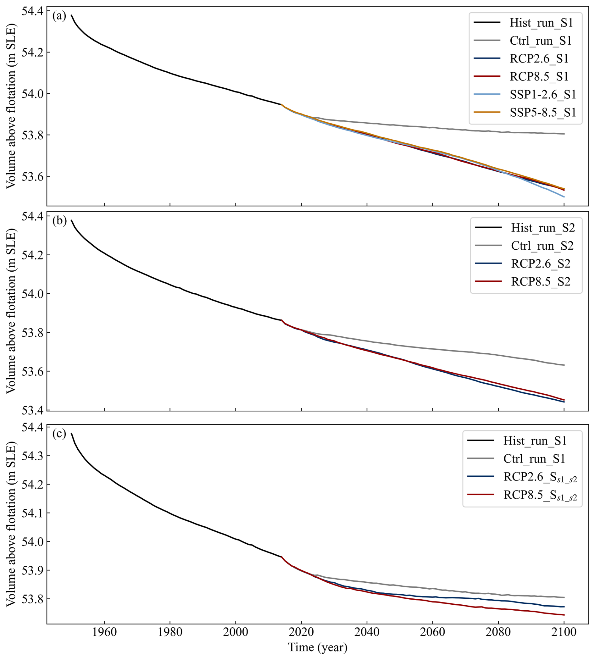
Figure A1 Ice volume above flotation (VAF) during spin-up and projection for (a) S1, (b) S2, and (c) S_{S1_S2} simulations. Black lines denote the historical spin-up, coloured lines show projections under RCP/SSP scenarios (light blue, red, dark blue, orange) and a constant-climate control run (grey).

To further assess whether a potential shock arises from the S1 initial state to S2 forcing during the projection in S1 simulations, we have introduced a general equation for the melt rate calculation (Eqs. A1 and A2): From the S2 projection, we extracted the annual oceanic forcing (S_{2_proj}; time, x, y) and subtracted the corresponding S2 initial state (S_{2_init}; x, y) to obtain a perturbation ΔS (time, x, y; Eq. A1). This ΔS was then added to the S1 spin-up (S_{1_init}; x, y) to construct a synthetic forcing S_{S1_S2} (time, x, y; Eq. A2) that represents the absolute ocean state under the S2 projection anomaly imposed on the S1 spin-up:

$$\begin{array}{}\text{(A1)}& {\displaystyle }\mathrm{\Delta }S=S_{\mathrm{2}\mathrm{\_}\mathrm{proj}}-S_{{\mathrm{2}}_{\mathrm{init}}},\text{(A2)}& {\displaystyle }{S}_{\mathrm{S}\mathrm{1}\mathrm{\_}\mathrm{S}\mathrm{2}}=S_{\mathrm{1}\mathrm{\_}\mathrm{init}}+\mathrm{\Delta }S\end{array}$$

Using this S_{S1_S2} forcing, we performed an additional projection starting from the S1 initial state. The resulting VAF time series (Fig. A1c) again shows no abrupt change, confirming the absence of a forcing shock. This can be attributed to two factors: (i) our projections are driven by absolute oceanic temperature and salinity, not anomalies; this ensures that the basal melt rates calculated from Eq. (2) respond directly to the full ocean state rather than to a perturbation. Although abrupt changes in the input forcing could theoretically affect ice-sheet evolution, the CMIP5 and CMIP6 climate forcing datasets used in our projections do not exhibit such abrupt shifts. (ii) The constant parameters values in the S2 parameterization are derived from in-situ observations or empirically calibrated against them, ensuring that the resulting basal melting closely matches the observations. Furthermore, in Fig. A1, the change in the slope of ice volume around 2015 likely indicates a discontinuity that appears to arise from the applied climate forcing rather than from the change in basal melting scheme, so it does not affect the difference between the two cases. In summary, no such shock is detected in the S1 simulated results when transitioning from the S1 initial state to S2 forcing.