Anticipating CRISTAL: an exploration of multi-frequency satellite altimeter snow depth estimates over Arctic sea ice, 2018–2023

The EU and ESA plan to launch a dual-frequency Ku- and Ka-band polar-orbiting synthetic aperture radar (SAR) altimeter, the Copernicus Polar Ice and Snow Topography Altimeter (CRISTAL), by 2027 to monitor polar sea ice thickness (SIT) and its overlying snow depth, among other applications. However, the interactions of Ku- and Ka-band radar waves with snow and sea ice are not fully understood, demanding further research effort before we can take full advantage of the CRISTAL observations. Here, we use three ongoing altimetry missions to mimic the sensing configuration of CRISTAL over Arctic sea ice and investigate the derived snow depth estimates obtained from dual-frequency altimetry. We apply a physical model for the backscattered radar altimeter echo over sea ice to CryoSat-2's (CS2's) Ku-band altimeter in SAR mode and to the SARAL mission's AltiKa (AK) Ka-band altimeter in low-resolution mode (LRM), and then we compare it to reference laser altimetry observations from ICESat-2 (IS2). ICESat-2 snow freeboards (snow + sea ice) are representative of the air–snow interface, whereas the radar freeboards of AltiKa are expected to represent a height at or close to the air–snow interface, and CryoSat-2 radar freeboards are expected to represent a height at or close to the snow–ice interface. The freeboards from AltiKa and ICESat-2 show similar patterns and distributions; however, the AltiKa freeboards do not thicken at the same rate over winter, implying that Ka-band height estimates can be biased low by 10 cm relative to the snow surface due to uncertain penetration over first-year ice in spring. Previously observed mismatches between radar freeboards and independent airborne reference data have frequently been attributed to radar penetration biases, but they can be significantly reduced by accounting for surface topography when retracking the radar waveforms. Waveform simulations of CRISTAL in its expected sea ice mode reveal that the heights of the detected snow and ice interfaces are more sensitive to multi-scale surface roughness than to snow properties. For late-winter conditions, the simulations suggest that the CRISTAL Ku-band radar retrievals will track a median elevation 3 % of the snow depth above the snow–ice interface because the radar return is dominated by surface scattering from the snow–ice interface which has a consistently smoother footprint-scale slope distribution than the air–snow interface. Significantly more backscatter is simulated to return from the air–snow interface and snow volume at Ka band, with the radar retrievals tracking a median elevation 10 % of the snow depth below the air–snow interface. These model results generally agree with the derived satellite radar freeboards, which are consistently thicker for AltiKa than CryoSat-2, across all measured snow and sea ice conditions.

1 Introduction

The Arctic marine system is one of the fastest-changing environments on Earth. Since the 1980s, the area of Arctic sea ice at the end of the summer melting season has approximately halved (Stroeve and Notz, 2018), while around three-quarters of the ice volume has disappeared (Kwok, 2018). The latest synthesis of climate model projections in the IPCC's Sixth Assessment Report suggests at least one practically ice-free summer in the Arctic is likely before 2050, regardless of the CO₂ emission scenario (Fox-Kemper et al., 2021). However, the spread in the projected timing of a regularly ice-free Arctic spans more than 30 years (Notz and Community, 2020). Much of this uncertainty comes from the structure of the sea ice component of the climate model (Bonan et al., 2021), and the Coupled Model Intercomparison Project (CMIP) Phase 6 ensemble does not reproduce the observed patterns of pan-Arctic sea ice thickness (SIT) accurately (Watts et al., 2021). According to Massonnet et al. (2018), the “current main obstacle to reducing uncertainties in projected sea ice volume or area trends is not the complexity of the models used, but rather the lack of long-term and reliable estimates of sea ice volume that can be used to constrain their projections.” Upgrading the observational SIT record will benefit climate model projections, improve the initialization of seasonal sea ice forecasts (e.g., Bushuk et al., 2017), and provide enhanced understanding of the Arctic's fast-changing sea ice mass and energy budgets.

The EU and ESA plan to launch a new Sentinel Expansion Mission, the Copernicus Polar Ice and Snow Topography Altimeter (CRISTAL), by 2027 to continue and enhance the record of spaceborne sea ice thickness observations in the Arctic (Kern et al., 2020). The observations from CRISTAL will build on a legacy of pan-Arctic SIT generated from the polar-orbiting ESA CryoSat-2 (CS2) mission since 2010 (e.g., Landy et al., 2022) and from historic radar altimeters (ERS-1/-2 and ENVISAT RA-2) with sub-Arctic coverage since 1995 (e.g., Bocquet et al., 2023). Complementary observations of pan-Arctic sea ice thickness have also been produced from the polar-orbiting NASA ICESat (2003–2009) and ICESat-2 (IS2; 2018 onwards) spaceborne laser altimetry missions (Kwok and Cunningham, 2008; Petty et al., 2023a). CRISTAL will carry a dual-frequency interferometric Ku- and Ka-band synthetic aperture radar (SAR) altimeter, with the goal to produce profiles of SIT at ∼250 m intervals along the track of the satellite with conventional delay-Doppler processing and <80 m with fully focused processing (Kern et al., 2020). The dual-frequency sensor is motivated by the assumption that Ku-band pulses penetrate through the snow layer on sea ice (e.g., Beaven et al., 1995), whereas Ka-band pulses scatter at the upper snow surface or layer (Guerreiro et al., 2016). This allows snow depth to be estimated from the height difference of the backscattered echoes. One of the largest sources of uncertainty in state-of-the-art SIT datasets comes from the snow load, which is conventionally obtained from a climatology (e.g., Warren et al., 1999) or estimated from an external source (such as fused climatology and passive-microwave-derived estimates or reanalysis-based accumulation models) to convert the altimeter's freeboard measurement to an estimate of SIT (Tilling et al., 2018; Mallett et al., 2021; Glissenaar et al., 2021). If the snow depth can be accurately measured by CRISTAL, concurrently with the measured sea ice freeboard, then uncertainty in the derived SIT may start approaching the 0.15 m on a 25 km length scale targeted by the mission (Kern et al., 2020; compared to the typical >0.5 m uncertainty on CryoSat-2 SIT estimates).

The basic assumptions of radar backscatter that have motivated the configuration of the dual-frequency CRISTAL payload are significantly more complex in reality. A variety of studies based on theoretical methods (Nandan et al., 2017, 2020; Tonboe et al., 2021; Meloche et al., 2024), in situ (or surface-based) radar (Willatt et al., 2009, 2023; Stroeve et al., 2020; Nandan et al., 2023), airborne radar (Willatt et al., 2011; King et al., 2018; de Rijke-Thomas et al., 2023), and satellite radar observations (Ricker et al., 2015; King et al., 2015; Nab et al., 2023) have challenged the assumption that spaceborne Ku-band radar altimetry (e.g., CryoSat-2) can accurately detect the height of the snow–ice interface over snow-covered sea ice floes. It has been suggested that CryoSat-2 may be sensitive to a radar scattering distribution with mean height within the snowpack, 60 %–90 % deep in the snow relative to the air–snow interface (Armitage and Ridout, 2015; Lawrence et al., 2018; Nab et al., 2023; Landy et al., 2022), implying that CryoSat-2 radar freeboards are consistently biased thick if there are not strong competing biases. Moreover, studies investigating coincident satellite observations from CryoSat-2 and the CNES/ISRO Ka-band altimeter mission SARAL AltiKa (AK) have challenged the assumption that Ka-band radar freeboards accurately represent the height of the air–snow interface over sea ice (Armitage and Ridout, 2015; Lawrence et al., 2018). AltiKa may also, therefore, be sensitive to a radar scattering distribution with a mean height within the snowpack of 0 %–40 % of the snow depth (Guerreiro et al., 2016; Armitage and Ridout, 2015; Nab et al., 2023).

Radar pulse propagation at the Ku and Ka band depends on the electromagnetic characteristics of the snow and sea ice cover. The radar wave can be scattered at the air–snow and snow–ice interfaces, depending on the dielectric contrast between layers and the “radar-scale” millimeter–centimeter roughness of the interface, i.e., similar to the wavelengths of ∼2 cm at the Ku band and ∼8 mm at the Ka band (Kurtz et al., 2014; Kwok, 2014; Landy et al., 2019; de Rijke-Thomas et al., 2023; Meloche et al., 2024). The wave can also be scattered and absorbed within the snow volume, depending on the snow density, grain size, dielectric properties (moisture, related to brine content), and structure (wind crusts, ice lenses) (Nandan et al., 2017, 2023; Willatt et al., 2023). These surface and volume scatterers are then distributed over a range of heights, with respect to the spherical wavefront of the propagating pulse, by the large-scale (meters to thousands of meters) topography of the sea ice cover. A rougher surface topography produces a broader backscattered radar echo (Kurtz et al., 2014; Landy et al., 2020). This complex set of scattering mechanisms can produce a mean height of the backscattered radar intensity that does not exactly match the absolute mean height of the snow surface (at the Ka band) or the sea ice surface (at the Ku band), even in the case where the waves negligibly or totally penetrate the snowpack. Ka-band waves are theoretically 1–2 orders of magnitude more sensitive to snow volume scattering than Ku-band waves (Mätzler, 1998; Rémy et al., 2015), and AltiKa freeboards are generally thicker than CryoSat-2 freeboards (Armitage and Ridout, 2015); however, the relative radar penetration depth into snow may not always be 0 % at the Ka band and 100 % at the Ku band.

It is not only the geophysical properties of the target that affect the returning altimeter waveform. The sensor design and measurement geometry can affect the relative importance of each scattering mechanism, and different methods for interpreting the radar signal can impact derived geophysical parameters such as the sea ice surface height or freeboard. For instance, de Rijke-Thomas et al. (2023) recently showed that the portion of the Ku-band radar signal that is reflected at the snow–ice interface depends closely on the altitude of the altimeter, and on the roughness and slope distribution of the target sea ice. The coherent radar reflection from the snow–ice interface (rather than incoherent surface or volume scattering) becomes increasingly dominant as the observation altitude increases, up to a range of ∼0.1–1 km sufficient for the far-field condition to apply, or the surface slope distribution narrows. Furthermore, a “retracking” algorithm must be applied to estimate the average elevation of the target surface from the leading edge of the waveform (Quartly et al., 2019). For sea ice altimetry, the so-called radar freeboard is then determined from the difference in retracked heights between sea ice floes and local sea surface reference samples at leads (Ricker et al., 2014). The retracking algorithm applied to floes and leads is based on a set of assumptions for their characteristic scattering properties. A bias in the derived sea ice freeboard vs. some reference validation dataset may therefore come from a geophysical source (e.g., pulse attenuation in the snow volume) or from the interpretation of the measurement (e.g., invalid assumptions of the retracking algorithm) (Landy et al., 2020). It can be impossible to separate these sources of error without auxiliary information.

In spite of these challenges, there have been several attempts to produce pan-Arctic snow depth estimates from dual-frequency altimetry. Guerreiro et al. (2016) developed a methodology with CryoSat-2 observations processed in pseudo-low-resolution mode (LRM) to match the LRM AltiKa observations and calculated snow depth at satellite crossovers <3 d apart assuming 0 % and 100 % snow penetration at the Ka and Ku band, respectively. This altimetric snow depth (ASD) “KuKa” processing chain was later updated to compute snow depth composites from monthly gridded CryoSat-2 and AltiKa freeboards (Garnier et al., 2021), with a comparison to snow depth estimates from Operation Ice Bridge (OIB) taken between 2014–2018 indicating an R² score of 0.44. Alternatively, Lawrence et al. (2018) calibrated CryoSat-2 SAR and SARIn mode and AltiKa LRM observations with coincident observations of derived radar freeboard and laser freeboard from combined airborne lidar and snow-radar spring OIB data to align the satellite freeboards from each altimeter down and up to the snow–ice and air–snow interfaces, respectively (Lawrence et al., 2018). A similar comparison to OIB data produced an R² score of 0.38. The offsets to OIB were attributed to variable radar penetration rates into snow (Armitage and Ridout, 2015), surface roughness, and sampling differences between sensors. Calibrated freeboards averaged to monthly grids are differenced to produce KuKa snow depth estimates, after accounting for the delayed Ku-band wave propagation speed in snow. The dual-altimeter snow thickness (DuST) methodology has more recently been applied to produce pan-Arctic “KuLa” snow depth estimates from the difference between CryoSat-2 observations, with the same calibration to airborne freeboards applied, and ICESat-2 ATL10 observations as part of the ESA Polar+ Snow on Sea Ice Project. Kwok et al. (2020) and Kacimi and Kwok (2022) also estimated pan-Arctic KuLa snow depths from the difference between uncalibrated CryoSat-2 and ICESat-2 observations, showing thinner depth estimates than the long-term snow depth climatology described in Kwok and Cunningham (2015). KuLa snow depth products have shown evidence for snow accumulation of 10 cm or more over winter and spring, matching expectations from reanalysis precipitation (Kwok et al., 2020), whereas KuKa products exhibit a much lower rate of seasonal accumulation (Lawrence et al., 2018; Garnier et al., 2021).

Here, we exploit the overlap in Arctic observations by the CryoSat-2, AltiKa, and ICESat-2 missions, at latitudes up to 81.5° N after October 2018, to examine how each sensor detects the freeboard of the snow, sea ice, or something in between. We use a waveform modeling method to simulate the theoretical radar return from rough snow and ice surfaces at the Ku and Ka bands, then we use these simulations to inform the retracking of surface height from CryoSat-2 and AltiKa, respectively. Monthly winter freeboards from CryoSat-2, AltiKa, and ICESat-2 are intercompared and used to derive two different estimates of the snow depth, which are then evaluated against independent snow depth data. Satellite laser/radar surface roughness estimates and radar backscattering coefficients, together with airborne estimates for the sea ice and snow freeboard, are used to investigate the wave-scattering mechanisms behind differences in sensors. Finally, we consider lessons learned from these multi-frequency observations in advance of the CRISTAL mission launch.

2 Data

2.1 CryoSat-2 SIRAL observations

The SAR Interferometric Radar Altimeter (SIRAL) on board CryoSat-2 combines a pulse-limited Ku-band radar altimeter with synthetic aperture and interferometric signal processing. The footprint of the sensor is therefore pulse-Doppler-limited ∼300 m along the track and pulse-limited to ∼1700 m across the track of the beam, with observations at ∼300 m intervals (Wingham et al., 2006) available up to a latitudinal limit of 88° N. Here, we use the Level-1B (L1B) SAR- and SARIn-mode Baseline E observations, obtained from the open ESA dissemination server at ftp://science-pds.cryosat.esa.int/ (last access: 9 August 2023), from October 2018 to April 2023, limited by the time period of ICESat-2 data (see Sect. 2.3) and covering the region north of 50° N. The L1B waveform observations from the larger 240 m range window in SARIn mode are truncated to match the 60 m range window of the SAR mode, and observations from the two modes are then treated identically. It is important to note that the range resolution of the altimeter is 0.47 m; however, the waveforms in the ESA L1B product are sampled at 0.23 m after zero padding is applied prior to the range FFT (Smith and Scharroo, 2014) to prevent aliased sampling of specular radar returns. This should lead to improved waveform fitting of lead echoes (see Sect. 3.3).

2.2 SARAL AltiKa observations

The AltiKa on board the Satellite with ARgos and ALtika (SARAL) is a Ka-band radar altimeter, with a pulse-limited footprint of ∼1400 m and a beam-limited footprint of ∼8 km, producing observations at 170 m intervals (Verron et al., 2015). It is primarily a sea-level monitoring mission, with a latitudinal limit of 81.5° N. Here, we use the L1B LRM mode Geophysical Data Record (sgdr_f) observations available from the AVISO Altimetry dissemination server at ftp://ftp-access.aviso.altimetry.fr (last access: 27 March 2024), from October 2018 to April 2023, and covering the Arctic region north of 50° N. The range resolution of the altimeter is 0.30 m.

2.3 ICESat-2 ATLAS observations

The Advanced Topographic Laser Altimeter System (ATLAS) on board ICESat-2 operates with a split-beam configuration of three 532 nm laser beam pairs, each including a strong and a weak beam. The beam pairs are spaced ∼3 km across the track of the sensor, with 90 m across-track and 2.5 km along-track separation between each strong and weak beam (Markus et al., 2017). The high pulse-repetition frequency produces laser pulses every ∼70 cm along track with a footprint diameter of ∼11 m. Here, we use the Level-3B ATL20 Version 4 Daily and Monthly Gridded Sea Ice Freeboard product available from NSIDC at Petty et al. (2023b), from October 2018 to April 2023. The laser freeboard is produced by aggregating 150 photons along a beam, determining the sea ice height from the photon distribution of this segment, and finding the height difference to a reference sea surface height determined from the photon distribution at local lead points (within 10 km along-track sections for each beam) (Kwok et al., 2019b). For ATL20, the along-track freeboards are aggregated at daily and then monthly timescales onto a 25 km×25 km Polar Stereographic North projection grid across the Arctic, which we resample onto an EASE2 grid using nearest-neighbor interpolation. Only the three strong beams are used to produce ATL20. To obtain an estimate for the surface roughness that is compatible with ATL20 and on a similar scale to the CryoSat-2 observations, we use the Level-3A ATL07 Version 6 Sea Ice Height product available from NSIDC at Kwok et al. (2023). Roughness is estimated from the standard deviation of surface heights from the central strong beam within 25 km along-track sections. Samples are removed if the section contains <100 heights and are then binned onto the same 25 km EASE2 grid.

Furthermore, we use the ICESat-2 Arctic Sea Ice Surface Topography data Version 2.1 from the University of Maryland–Ridge Detection Algorithm (Duncan and Farrell, 2022), available at https://zenodo.org/records/7129192 (last access: 3 December 2023). We use the snow surface roughness parameter, obtained from a ridge detection scheme applied to ATL03 photon heights, for April 2019, to support the simulation of CRISTAL waveforms (Sect. 5.4).

2.4 Reference observations

To validate our satellite snow depth estimates and investigate the radar backscatter mechanisms potentially introducing biases into freeboard observations, we compare the satellite measurements to several airborne and in situ datasets. This includes a set of reference observations prepared and gridded by AWI for the ESA Polar+ Snow on Sea Ice Project: (i) snow depth information from airborne radar data is available in the AWI IceBird Winter 2019 campaign dataset (Jutila et al., 2022a), available at https://doi.org/10.1594/PANGAEA.966057 (Jutila et al., 2024), for April 2019. These data were processed with the PySnowRadar package (https://doi.org/10.5281/zenodo.4071947; King et al., 2020) based on the “peakiness” method described in Jutila et al. (2022b). (ii) Snow depth information collected manually with a magnaprobe along the two loops of the MOSAiC campaign Central Observatory transects, approximately weekly (Itkin et al., 2023), is available at https://doi.org/10.1594/PANGAEA.937781 (Itkin et al., 2021) for October 2019 to April 2020. (iii) Snow depth information processed from airborne radar data collected by the Center for Remote Sensing and Integrated Systems (CReSIS) at the University of Kansas, with the peakiness method and same PySnowRadar parameters as the IceBird data, is available at http://data.cresis.ku.edu/#SR (last access: 25 July 2024) for the five OIB flight campaigns on 6, 12, 19, 20, and 22 April 2019. A snow density of 300 kg m⁻³ was applied to derive the snow depths, consistent with the IceBird processing for reference dataset (1) but not with the application of time-dependent snow density for the satellite estimates (see below). This mismatch in snow density adds a small uncertainty to the validation results. The reference observations are gridded onto a monthly 25 km EASE2 (Brodzik et al., 2012) projection to match the satellite data.

Furthermore, we use the laser-scanner-derived snow (or total) freeboard observations from the April 2019 OIB and AWI airborne campaigns, along with the airborne snow depth estimates, to estimate the expected Ku-band freeboard – under the assumption of total radar penetration – following the approach of Lawrence et al. (2018). The sea ice freeboard is calculated by subtracting the airborne radar snow depths from the laser scanner snow freeboards and then converted to the expected Ku-band radar freeboard by accounting for the delayed radar wave propagation through snow (assuming a snow density of 300 kg m⁻³). The laser scanner snow freeboard observations represent the expected Ka-band radar freeboard, under the assumption of zero radar penetration.

3 Methods

3.1 Basis of the approach

The basis for the waveform modeling approach (the Lognormal Altimeter Retracker Model, LARM) is to fit a physical model for the backscattered radar altimeter echo to observed altimeter waveforms and obtain, through the model inversion (Landy et al., 2020), estimates for the retracked snow–ice interface elevation (CryoSat-2), air–snow interface elevation (AltiKa), or sea surface height at leads (both sensors). A mean sea surface (MSS) model, here the DTU21 solution (Baltazar Andersen et al., 2023), is subtracted from the retracked heights to calculate sea ice height and sea surface height anomalies (SSHAs). The radar freeboard is calculated from the height difference between the ice floe elevation anomalies and an estimate for the SSHA interpolated (see below) between tie points from nearby leads along the orbital track of the satellite. Radar freeboards from a given month are then binned and averaged on a 25 km×25 km EASE2 grid that covers the entire Arctic and are finally corrected for the delayed travel speed of the CryoSat-2 Ku-band radar wave through snow (Mallett et al., 2020) to produce estimates for the pan-Arctic snow depth, following, e.g., Lawrence et al. (2018). These steps are explained in more detail below.

The fundamental assumption of the method is that forward model solutions for the CryoSat-2 Ku-band SAR echo or AltiKa Ka-band LRM echo adequately represent the height of the snow–ice or air–snow interface, respectively, based on the physical mechanisms scattering or reflecting the radar waves at each frequency. Here we take the simple but necessary approach to model both Ku-band and Ka-band radar waveforms as if the backscatter is returned from a single backscattering surface, assumed to represent the snow–ice and air–snow interfaces, respectively. Several studies have called this assumption into question, as described in the Introduction. For instance, snow volume scattering, attenuation by brine-wetted snow, new snowfall, and variations in radar-scale surface roughness may impact the height of the maximum radar backscattering intensity at each frequency. In cases where our fundamental assumption of a single scattering surface is invalidated and/or the model inadequately reproduces the true scattering response of the radar wave, we will obtain a bias in the retracked elevation.

The alternative option would be to forward model the full combination of possible surface and snow volume scattering mechanisms; e.g., see Sect. 5.4. However, any influential model parameter that cannot be constrained by additional data (e.g., snow depth, density, grain size, dielectric properties) would need to be a free parameter in the model inversion. In this scenario, the inversion of a larger number of free parameters based on a single waveform would consequently be very uncertain with high degeneracy between certain model parameters, for example, the surface roughness and snow depth (de Rijke-Thomas, 2019), so this is currently not considered a viable option.

3.2 Radar waveform modeling

In the case of a single backscattering surface, the radar altimeter echo model is parameterized by four terms: A, the scaled waveform amplitude; t₀, the tracking point of the mean radar scattering surface (or “epoch”); σ, the surface topography root-mean-square height; and s_rms, the millimeter–centimeter “radar-scale” roughness. This is assuming that variations in the radar antenna parameters (e.g., satellite altitude, off-nadir pointing angle) have a negligible impact on the shape of the sea ice waveform return and can be ignored.

We use the Facet-Based Echo Model (FBEM) which simulates the radar altimeter echo as the integral of the power backscattered from a tetrahedral mesh representing the sea ice surface topography (Landy et al., 2019). The FBEM is available as an open-source MATLAB code at https://github.com/jclandy/FBEM (last access: 3 March 2023). The scattering mechanisms are characterized for each facet of the mesh. Backscatter from the air–snow or snow–ice interface is obtained from the sum of the scattered and reflected components, simulated with the Integral Equation Model (IEM; Fung and Chen, 2004) and Kirchoff physical optics approximation (Fung and Eom, 1983), respectively. The balance between scattering and reflection depends on the radar frequency and radar-scale roughness of the surface (Landy et al., 2020). A waveform simulation uses a single radar-scale roughness for every facet; however, the backscatter from each facet still varies nonlinearly as a function of the facet's local slope angle – being larger for smaller slope angles that face the radar (Landy et al., 2020; Nandan et al., 2023). This means level ice facets contribute disproportionately to the total backscattered echo, compared to sloped facets (i.e., ridges), and reduce the height of maximum backscattered radar intensity compared to the true mean floe surface height (de Rijke-Thomas et al., 2023). This is analogous to the radar altimetry sea state bias over the ocean (Tran et al., 2010).

The large-scale topographies of the air–snow or snow–ice interfaces are characterized by a lognormal probability density function of the height distribution, following Landy et al. (2020). A single lookup table of Ku-band SAR altimeter echoes is simulated from FBEM for sea ice and lead surfaces with lognormal height PDF, σ ranging from 0 to 1 m, and s_rms ranging from 0 to 6 mm, as described in Landy et al. (2020). Radar antenna parameters are characterized for the CryoSat-2 SIRAL instrument (Landy et al., 2019). Examples for the modeled SAR echoes with fixed s_rms of 2 mm but varying σ are shown in Fig. 1a. The parameter s_rms controls the magnitude of the radar backscatter from the surface and the incidence angle dependence of the backscattering coefficient, with a smaller value producing a higher power and a peakier waveform return. The parameter σ controls the roughness of the large-scale sea ice topography and principally affects the width of the waveform leading edge. When s_rms=2 mm and σ=0 (orange waveform), the echo represents the approximate reflection of the transmitted pulse. Such peaky waveforms are characteristically produced when the radar signal is reflected from leads in sea ice. The radar tracking point t₀ defines the mean elevation of the surface height distribution within the radar footprint. Zero time in Fig. 1 represents t₀ and is crossed at a different amplitude of the waveform leading edge power depending principally on σ. This implies that the relative retracking amplitude should decrease as the large-scale roughness of the snow–ice interface increases, from around 98 % for σ=0 % to 67 % for σ=0.5 m (i.e., tracing down the t=0 line in Fig. 1a).

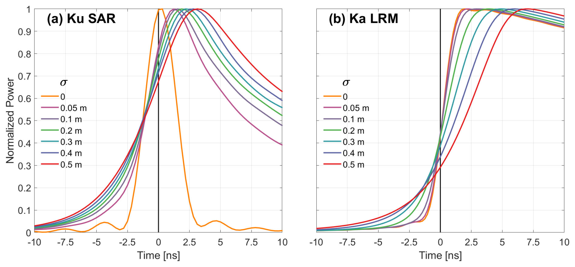
Figure 1 Radar echo simulations for a single backscattering interface (snow or sea ice) with a lognormal roughness height distribution and different roughness standard deviations σ in (a) Ku-band SAR-mode with radar sensing parameters from CryoSat-2 SIRAL and in (b) Ka-band LRM-mode with radar sensing parameters from AltiKa SARAL. For these examples, s_rms is held at a fixed 2 mm. Zero time represents the radar tracking point t₀.

A single lookup table of Ka-band LRM altimeter echoes is also simulated from FBEM for sea ice and lead surfaces with lognormal height PDF, σ ranging from 0 to 1 m, and s_rms ranging from 0 to 6 mm. Radar antenna parameters are characterized for the AltiKa SARAL instrument, based on https://directory.eoportal.org/web/eoportal/satellite-missions/s/saral (last access: 26 September 2020). Examples for the modeled LRM echoes with fixed s_rms of 2 mm but varying σ are shown in Fig. 1b. The roughness of the large-scale sea ice topography σ appears to impact the width of the leading edge more in Ka-band LRM mode than in Ku-band SAR mode (e.g., Guerreiro et al., 2016; Fredensborg Hansen et al., 2021). The radar tracking point t₀ is also again crossed at a different amplitude of the waveform leading edge power depending on σ (i.e., tracing down the t=0 line in Fig. 1b). This implies that the relative retracking amplitude for LRM waveforms should also decrease as the large-scale roughness of the air–snow interface increases, from around 50 % for σ=0 % to 28 % for σ=0.5 m.

3.3 Waveform fitting and freeboard derivation

We use a least-squares fitting procedure to optimize the functional form of the modeled sea ice echo to observed CryoSat-2 or AltiKa waveforms. The fitting routine is based on the bounded trust region reflective algorithm (implemented through the MATLAB function lsqnonlin) to minimize the difference between the model fit and each observed power waveform, as described in Landy et al. (2020). A filtering routine is applied to exclude samples at major secondary peaks, on the waveform trailing edge from the model fit (Fig. 2). This routine identifies all waveform peaks between the primary peak and noise floor (on the waveform trailing edge) and then removes samples if the area of the peak is above a threshold value. The routine is identical between CryoSat-2 and AltiKa, but the thresholds are different. Initial values for the four free parameters are determined as t₀ at 70 % of the waveform leading edge power, A at the waveform maximum, and σ and s_rms corresponding to the modeled echo from the lookup table with a peakiness value closest to the peakiness of the observed waveform (Landy et al., 2020). At the end of the fitting procedure, we obtain optimal estimates for all four parameters. Examples for the best-fitting modeled echoes to sea ice floe surfaces and leads, for both CryoSat-2 and AltiKa waveforms, are shown in Fig. 2 along with their associated parameters. It is evident that the large-scale topography σ and small-scale roughness s_rms are both larger for the floe surfaces than for leads. It is also notable that the zero padding applied to CryoSat-2 SAR waveforms doubles the range sampling, without adding any new information (Smith and Scharroo, 2014), but provides an improved constraint on the elevation of specular leads than can be obtained from the specular AltiKa LRM waveforms at their native bandwidth-limited range resolution (Fig. 2b and d).

Figure 2 Best-fitting model echoes to observed radar waveforms from (a, b) CryoSat-2 SAR mode and (c, d) AltiKa LRM mode. Panels (a) and (c) show model fits to characteristic diffuse-type waveforms returned from a rough sea ice and/or snow surface. Panels (b) and (d) show model fits to characteristic specular-type waveforms returned from smooth ocean lead surfaces. The dashed lines mark the “epoch” or radar retracking point, i.e., the mean level of the scattering surface, with respect to the echo maxima. Hollow samples at major secondary peaks are discarded from the waveforms during fitting.

The satellite range is obtained from half the retracked two-way travel time to the surface multiplied by the speed of light. The surface height relative to the WGS84 ellipsoid is then obtained from the satellite altitude minus the range and is subsequently corrected for atmospheric effects (dry and wet troposphere, ionospheric delay, inverse barometer correction) and geophysical effects of the ocean (ocean tide, loading tide, pole tide) using corrections provided in the data products. The corrections can therefore be different between sensors, with negligible impact on the results (Ricker et al., 2016). A conservative low-pass filter is applied to the along-track height profile to remove residual sea surface topography (with a horizontal wavelength greater than 200 km) that is not removed by the geophysical corrections.

Waveforms are separated into three classes (sea ice floes, leads, and ocean) with a simple thresholding technique based on several waveform shape parameters. No class is used for “ambiguous” waveforms. For CryoSat-2, the parameter thresholds are based on results from Müller et al. (2023) who showed that previous classification schemes for CryoSat-2 generally assigned observations over thin sea ice to the ambiguous class, potentially biasing the derived sea ice freeboard high by omitting them. Observations are classed as leads where the radar backscattering coefficient (σ⁰) is > 23 dB in SAR mode and > 24 dB in SARIn mode, the pulse peakiness (PP) is > 0.258 in SAR mode and > 0.254 in SARIn mode, and the leading edge width (LEW) is < 4.69 ns in SAR mode and < 6.56 ns in SARIn mode (Hendricks et al., 2021). Observations are classed as ocean where σ⁰ < 2.5 dB, the stack standard deviation (SSD) > 55, or the sea ice concentration (from the OSISAF product OSI-401-d) < 15 %. All remaining valid observations are classified as sea ice. For AltiKa, the parameter thresholds are based on Armitage and Ridout (2015) and Zakharova et al. (2015). Observations are classified as leads where σ⁰ > 15 dB, the PP > 0.156, and the LEW < 4.58 ns. Observations are classed as ocean where σ⁰ < 2.5 dB or the sea ice concentration < 15 %. All remaining valid observations are classified as sea ice.

The SSHA is obtained at ice-covered locations from a linear interpolation between lead elevations, along the orbit of the satellite and smoothed on a 25 km length scale, as described in Landy et al. (2020). All sea ice observations >300 km from their nearest lead are discarded. Along-track radar freeboards are calculated from the elevation difference between sea ice floes and the interpolated SSHA. An estimate for the SSHA uncertainty at a lead location is made from the standard deviation of lead elevations within a 50 km along-track window around the lead. At ice floe locations, the SSHA uncertainty is estimated from the uncertainty at proximal leads, scaled by the inverse of the squared distance to the nearest lead, up to a maximum of 10 cm at 300 km.

3.4 Snow depth estimation and intercomparison

The radar freeboards for both CryoSat-2 and AltiKa are gridded, at monthly intervals, onto the same 25 km×25 km EASE2 projection Arctic grid using a binned weighted mean algorithm, with each freeboard observation weighted inversely by its absolute uncertainty. The SSHA uncertainty is gridded with the same method. The range error on a single 20 Hz CryoSat-2 observation is estimated to be 10 cm for SAR mode and 14 cm for SARIn mode (Wingham et al., 2006), and the range error on a single 40 Hz AltiKa LRM mode observation is estimated to be 5 cm (Dettmering et al., 2015). This range error is considered to be fully random, incorporating speckle and retracking error from the waveform fitting process; however, there may be other systematic errors, such as retracker bias, that are not known and are thus not included. For a conservative estimate of the total radar freeboard uncertainty, we therefore sum the range error (multiplied by $\mathrm{1}/\sqrt{N}$ observations in a grid cell) and the mean gridded SSHA uncertainty in quadrature. After averaging to a 25 km scale, the precision on the gridded radar freeboards is around 2–3 cm (Fredensborg Hansen et al., 2024).

The ICESat-2 ATL20 monthly snow freeboard data are reprojected onto our EASE2 grid. We then estimate the snow depth in two ways: (i) from the height difference between CryoSat-2 and AltiKa, “KuKa”, and (ii) from the height difference between CryoSat-2 and ICESat-2, “KuLa”. We assume that the CryoSat-2 radar freeboards represent the elevation of the snow–ice interface (see Sect. 5.4 below), but this is not yet corrected for the delayed Ku-band wave propagation velocity through the snowpack. To derive estimates for the snow depth from the height difference in gridded freeboards, we therefore multiply by the height difference corresponding to the ratio of radar wave velocities in snow and free space (Lawrence et al., 2018) using Eq. (81) in Ulaby et al. (1986) Volume 3. The snow density is estimated to vary seasonally, between 266–329 kg m⁻³, from October to April, based on Mallett (2025). Snow depth uncertainty is derived from the radar freeboard uncertainties and their covariance for KuKa and from the radar and laser freeboard uncertainties and their covariance for KuLa following the method of Lawrence et al. (2018). Note that we do not calibrate the radar freeboards, as in Lawrence et al. (2018), so uncertainties on the calibrations are also omitted from the uncertainty calculation.

4 Results

We firstly analyze the basin-wide patterns and distributions of the CryoSat-2 (CS2) and AltiKa (AK) radar freeboards and ICESat-2 (IS2) laser freeboards in 2 selected months: December 2018, in the early stages of the snow accumulation season but with sea ice close to its maximum extent, and April 2019, towards the end of the same snow accumulation season. We then analyze the differences between the KuKa and KuLa versions of the snow depth, including the seasonal differences in estimated snow accumulation rate. Finally, we intercompare the derived snow depths with airborne and in situ snow depth measurements collected between 2019–2020.

4.1 Radar and laser freeboard intercomparison

The CryoSat-2 radar freeboard observations in December and April are thinner than both the AltiKa radar and ICESat-2 snow freeboards. All three datasets show relatively thicker freeboards over the MYI than over the FYI zone (Figs. 3a–c and 5a–c). The mean of the CS2 freeboard distribution is 3.7 and 5.3 cm in December and April, respectively, compared to 21 and 26 cm for AK and 18 and 30 cm for IS2 (Figs. 4a and 6a). Around half of the December CS2 freeboards south of 81.5° N are thinner than 3 cm, representing new ice forming recently in the marginal ice zone (MIZ). This threshold is approximately the lower freeboard detection limit of CryoSat-2 when using a physically based retracker (see Fig. 7 in Landy et al., 2020 and Fredensborg Hansen et al., 2024). Thicker AK and IS2 freeboards in the MIZ represent snow accumulating on newly forming sea ice (see Sect. 5.3).

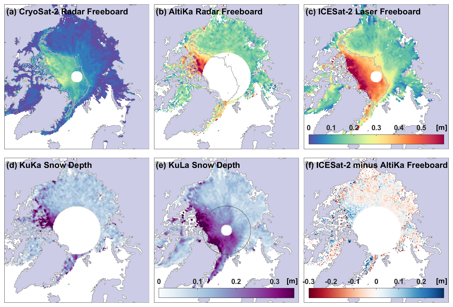
Figure 3 Example of the CryoSat-2 (a) and AltiKa (b) radar freeboards obtained from physical model waveform fitting in December 2018, with comparison to ICESat-2 (c) laser freeboards. Two estimates for the snow depth are obtained from a simple difference between KuKa (CryoSat-2 and AltiKa) freeboards (d) and KuLa (CryoSat-2 and ICESat-2) freeboards (e) corrected for the delayed Ku-band wave speed through the snow volume. A map of the difference between ICESat-2 and AltiKa freeboards is shown in panel (f). The gray lines in panels (a)–(c) show the boundary of the MYI zone based on the monthly mean sea ice type from OSI SAF (OSI-403-d).

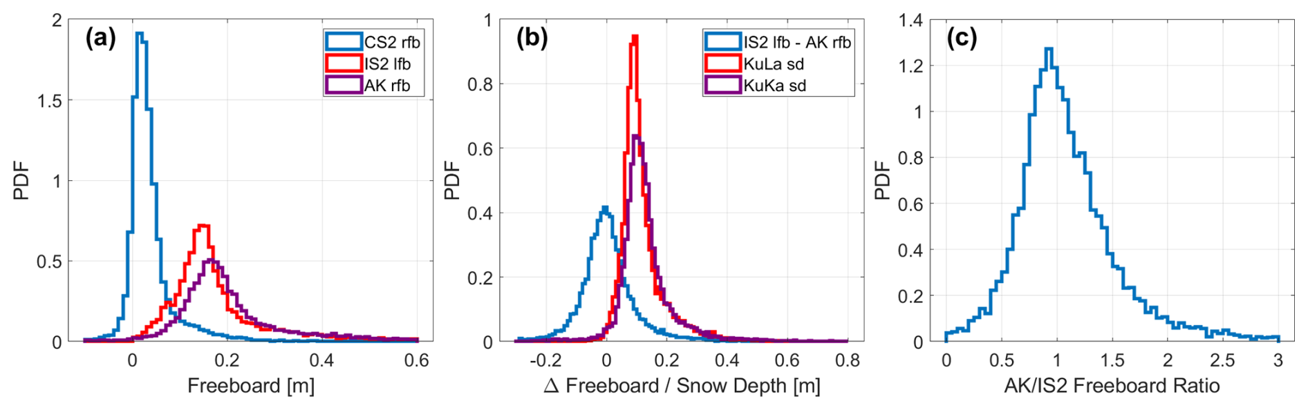
Figure 4 Comparison of the gridded radar freeboards (rfb) obtained from physical model waveform fitting applied to CryoSat-2 and AltiKa to laser freeboards (lfb) obtained from ICESat-2 in December 2018. (a) Freeboard distributions. (b) Derived snow depth (sd) distributions and the distribution of gridded differences between AltiKa and ICESat-2. (c) The AltiKa freeboards plotted as a ratio of the ICESat-2 freeboards. Note that distributions only cover the coinciding region of observations between the three sensors south of 81.5° N.

The AK and IS2 freeboards display many similarities in their regional variability, for example, thicker freeboards in the northern region of the Canadian Arctic Archipelago (CAA), in the Beaufort Sea, and in the Fram Strait. The transition in freeboard across the MYI tongue circulating into the Beaufort Sea, in particular, is captured by both AK and IS2 in December and April. It is evident, however, that the AK radar freeboards show more local spatial variability than the smoother patterns of the CS2 and IS2 freeboards, which may be attributable to higher uncertainty in the AltiKa LRM freeboard observations. All three sensors exhibit freeboard patterns in December that closely match the ice type zones mapped in the OSI-403-d product, with sharp gradients in freeboard across the MYI edge (Fig. 3a–c). It is notable that, by April, the clear separation by ice type is not preserved in the CS2 freeboards, and, while it is more obvious in the AK and IS2 freeboards, it is not in the Atlantic Sector, where the ice is more dynamic and seasonal ice thickening/snow accumulation might depend less on the ice type (Fig. 5a–c; see Sect. 5.3).

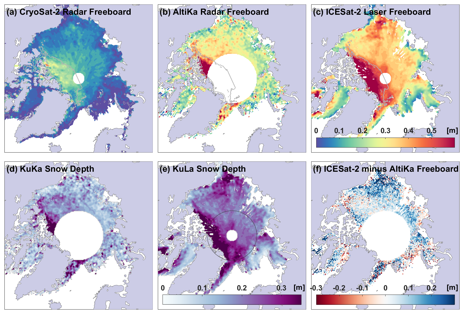
Figure 5 Same as Fig. 3 but for April 2019.

Figure 6 Same as Fig. 4 but for April 2019.

The CS2 radar freeboard distributions are narrower than the others, with ∼15 % of grid cells having near-zero or slightly negative freeboards, reflecting thinner sea ice floes loaded by surface snow (Figs. 4a and 6a). MYI freeboards are evident in the tails of the CS2 distributions thicker than ∼10 cm. The AK and IS2 freeboard distributions are both unimodal in December, but the IS2 distribution alone becomes bimodal by April, reflecting thickened IS2 freeboards in the Chukchi and East Siberian seas that are not observed in the AK data and only weakly observed in the CS2 data. Generally, the freeboard patterns from CS2 and IS2 are quite similar, albeit with different magnitudes. The thinnest CS2 freeboards (<5 cm) in the MIZ typically coincide with the thinnest IS2 freeboards (<10 cm) (Figs. 3a and c and 5a and c), where snow depth is expected to be thinnest over newly formed sea ice (see Sect. 5.3). Clear exceptions are in the Chukchi Sea, where IS2 freeboards thicken more than any other region between December 2018–April 2019 (Kwok et al., 2020), and in Baffin Bay, where the east–west gradient in IS2 freeboards is not so evident in the CS2 freeboards (Glissenaar et al., 2021). The IS2 freeboards also show a broader distribution of thickness (std dev 15.3 cm) across the entire Arctic in April than the CS2 freeboards (std dev 6.7 cm).

4.2 Snow depth intercomparison

The KuKa and KuLa snow depths are shown in Fig. 3d and e and 5d and e. There are some clear similarities between the two products, including thicker derived snow depths over MYI north of Canada and in the Fram Strait than over FYI in the surrounding Arctic seas. The locations of thicker snow depths in the northern CAA and in the Beaufort Sea are very similar. However, the KuLa maps show more regional variability in snow depth than the KuKa maps, including within the first-year ice/MIZ regions, where snow depth is sensitive to freeze-up timing, strong snowfall events, and wind compaction/snow loss events (Webster et al., 2018). For instance, there is no clear gradient in snow depth at the Barents Sea or Baffin Bay ice edge in the December KuKa product (Fig. 3d). The KuKa snow depths exhibit more local variability on the scale of tens of kilometers, reflecting the variability in the AK radar freeboards, whereas the KuLa snow depths exhibit smooth regional gradients in snow depth over scales of thousands of kilometers. The pan-Arctic (up to 81.5° N) snow depth distributions are relatively narrow and similar in December (Fig. 4) but diverge in April, with KuKa snow depths showing a mode at 15 cm and KuLa snow depths showing a broader peak with mode at 19 cm but a small secondary peak of thinner depths at ∼10 cm.

The height differences between AK and IS2 freeboards show some regional patterns. In December, IS2 is ∼3–4 cm thicker than AK over the MYI region north of Canada but generally similar to AK over FYI, albeit with local grid-cell scale differences (Fig. 3f). In April, AK freeboards generally underestimate those from IS2, by 3–15 cm, except around the ice edge (Fig. 5f). Figures 4c and 6c show that the distributions of the grid-cell freeboard ratio between AK and IS2 have a mode around 1 in December and around 0.85 in April. The shift in freeboard ratio for April is particularly caused by IS2 observing much thicker freeboards than AK in the Chukchi and East Siberian seas (Fig. 5f). The distributions are approximately Gaussian around these modal values, except from a tail of grid cells with higher ratio that gives the distributions a positive skew (skewness ∼1), where AK freeboards are 50 %–100 % thicker than those measured by IS2.

4.3 Seasonal snow accumulation

The time series of KuKa and KuLa mean snow depth and variability, across the five accumulation seasons, exhibit some clear differences (Fig. 7). Both time series show increasing snow depths through winter, with the exception of October to November, when large areas of newly forming sea ice with lower accumulated snow reduce the basin-wide mean. The mean and standard deviation of the snow depth are also both higher over MYI than FYI, for both products. However, the basin-wide standard deviation in the snow depth is around 8–13 cm for KuKa compared to 6–10 cm for KuLa. The rates of estimated snow accumulation are also quite different between the products, with a mean seasonal increase of 0.5 cm month⁻¹ for KuKa compared to 1.7 cm month⁻¹ for KuLa. The rate of snow accumulation for the KuKa product is implausibly low. For the KuLa product, the pan-Arctic mean rate of accumulation, including observations up to 88° N, is 1.6 cm month⁻¹ (Fig. A1). Relatively low rates of snow accumulation have been observed previously for CryoSat-2-AltiKa snow depth products (Lawrence et al., 2018; Garnier et al., 2021).

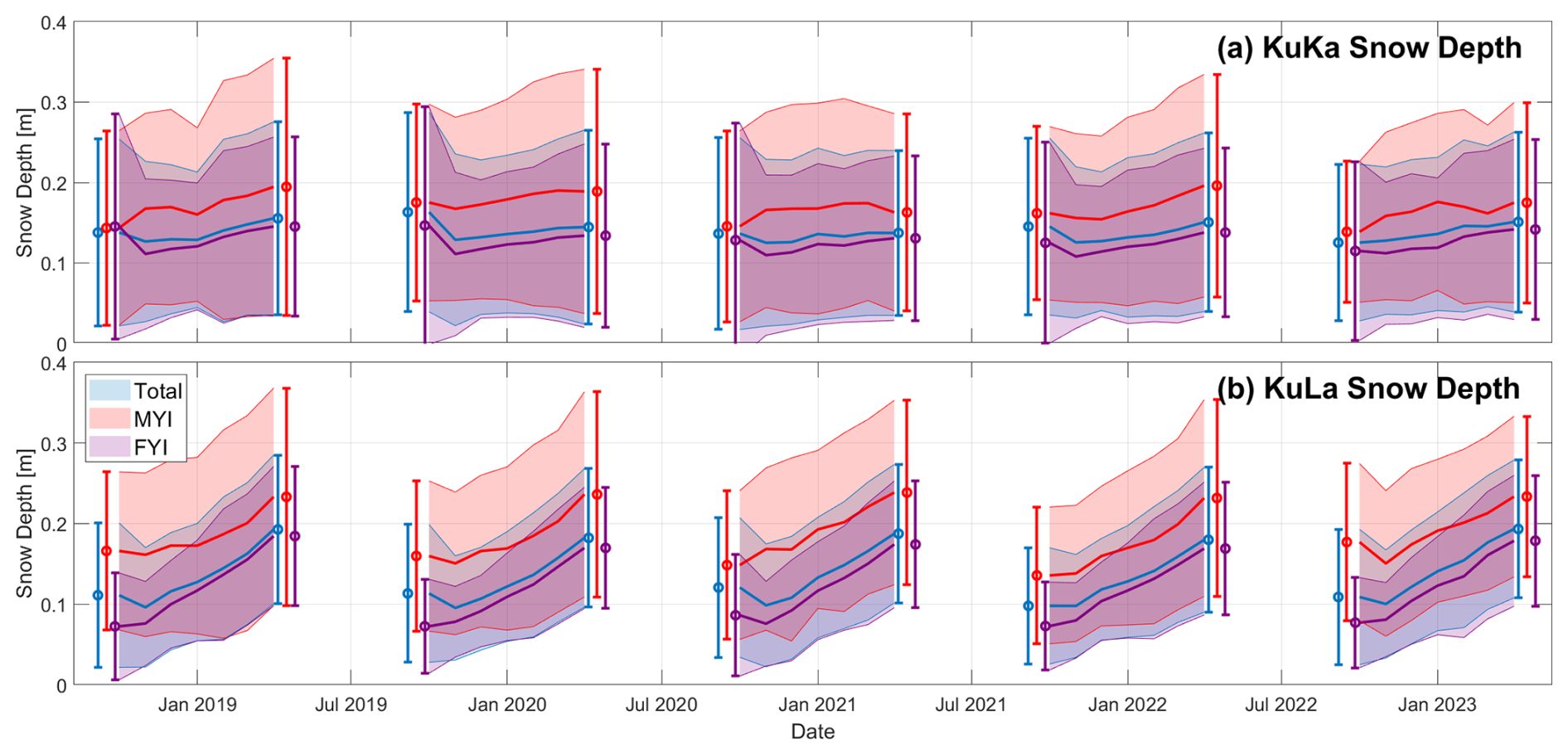
Figure 7 Time series for the seasonal change in snow depth obtained from (a) KuKa radar and (b) KuLa radar and laser freeboards over the 2018–2023 sea ice growth/snow accumulation seasons, for coincident data up to 81.5° N. The envelopes represent ± 1 standard deviation around the mean snow depth. The points and whiskers also show snow depths of ± 1 standard deviation around the mean at the start and end of each observation season. A second version of this figure, including KuLa observations up to 88° N, is shown in Appendix Fig. A1.

The KuLa snow depths, which offer near-basin-wide coverage, grow from around 8–18 cm over first-year ice and 17–26 cm over multi-year ice across the snow accumulation season (Fig. 7b). The accumulation of snow on MYI is slower than on FYI, however, at a mean accumulation rate of around 1.6 cm month⁻¹ on MYI vs. around 1.9 cm month⁻¹ on FYI. The interannual variability in KuLa snow depth is 0.4 and 0.6 cm, respectively, at the start and end of the snow accumulation season across these 5 years. This is significantly lower than the 3–7 cm interannual variability in snow depth obtained from a Lagrangian snow accumulation scheme (SnowModel-LG) and would make only a small contribution to the estimated interannual variability in sea ice thickness (20–30 cm) (Mallett et al., 2021).

4.4 Evaluation against independent observations

The satellite snow depths are compared with in situ observations and airborne snow depth estimates (see Sect. 2.4) in Fig. 8. It is important to note that KuKa observations are compared to reference data covering only N=50 of our 25 km×25 km grid cells in April 2019, with a low density of leads for some grid cells in the northern channels of the Canadian Arctic Archipelago. Our KuLa snow depths are compared to the same data plus additional reference data at higher latitudes covering a total of N=188 grid cells across 8 months. Each satellite product overestimates the reference snow depth by 2 cm, on average, and tends to overestimate the thinner snow depths over FYI, in particular. The KuKa product has a slope of 0.58 with respect to the reference data, meaning that it underestimates the spread of snow depths at a 25 km scale. The thinnest reference snow depths are overestimated and the thickest reference snow depths are underestimated by ∼5 cm. For KuLa also, reference snow depths from the thinnest category of 5–10 cm, collected during IceBird over FYI in the Beaufort Sea and from the MOSAiC Central Observatory in situ transects in fall, are consistently overestimated (Fig. 8). However, the slope of the KuLa product is 0.86 with respect to the reference data, meaning that it generally represents the spread of the snow depths at 25 km very closely. The KuLa product reasonably matches the magnitude and variability in the reference snow depths, with a correlation of 0.79 and an RMSE of 7 cm (Fig. 8). For fewer grid cells, south of 81.5° N, the KuKa product has a correlation of 0.70 and RMSE of 9 cm vs. the reference snow depths. When grid cells north of 81.5° N are excluded from the KuLa comparison, the correlation is 0.80 and RMSE is still 7 cm; however, the bias increases to 3 cm, and the slope reduces to 0.72.

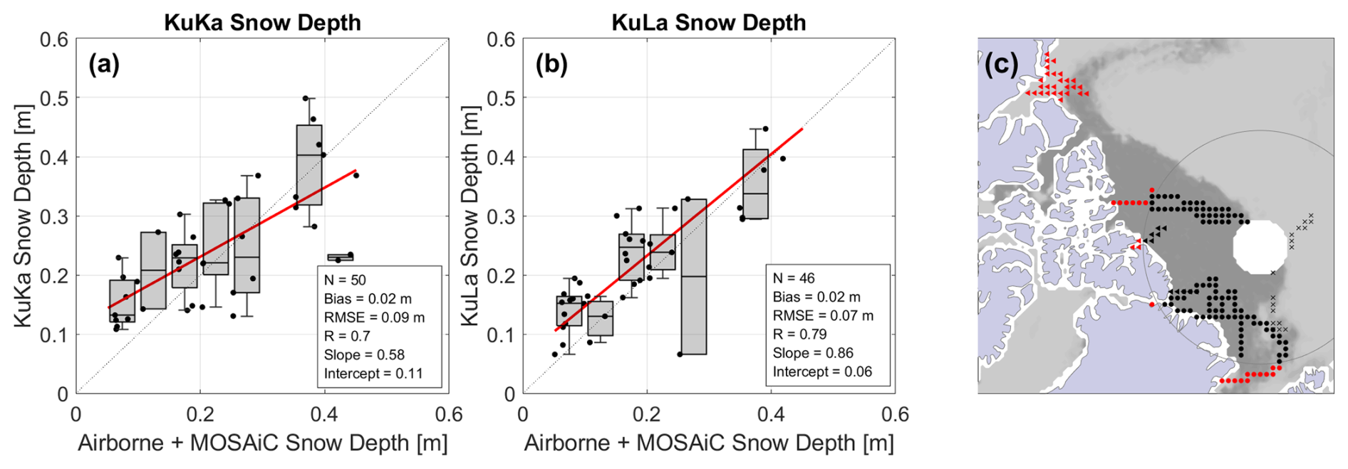
Figure 8 Intercomparison between snow depth estimates from (a) KuKa radar freeboards, (b) KuLa radar and laser freeboards, and independent snow depth observations. Box and whiskers are binned at 5 cm intervals. The map in panel (c) shows sea ice type from OSI-403-d, with MYI in dark gray and FYI in light gray, for April 2019, with the locations of data from OIB April 2019 (circles), IceBird April 2019 (triangles), and the MOSAiC Transect October 2019–April 2020 (crosses). Red samples are compared to KuKa and KuLa satellite snow depths, whereas black samples are compared only to KuLa snow depths.

5 Discussion

It is challenging to identify the source or sources of bias between the KuKa and KuLa snow depths in any given mont, and between each product and the reference snow depth data. Biases could be caused by (i) the height of maximum intensity of the Ku- or Ka-band radar backscatter not aligning with the snow–ice or air–snow interface, respectively, owing to radar penetration or surface-roughness-related effects; (ii) the ICESat-2 laser penetrating into the snowpack (Studinger et al., 2024) or possible lead height retrieval errors leading to uncertainties in the laser freeboards (Kwok et al., 2019a); (iii) our model for the radar altimeter not adequately simulating the true backscattered radar response in SAR or LRM mode; (iv) our model assumption of a single backscattering surface not being valid, owing to strong contributions from snow volume scattering or reflections from other interfaces than the one modeled; (v) inaccurate sample classification erroneously removing sea ice floe or including lead elevation measurements in the freeboard products (e.g., Petty et al., 2021; Fredensborg Hansen et al., 2021; Müller et al., 2023); or (vi) different orbital sampling between sensors and interpolation errors mapping observations to monthly pan-Arctic grids (Lawrence et al., 2019). The reference data themselves are also uncertain, especially measuring the thinnest and thickest snow depths (Kwok et al., 2017). Any one or a combination of these effects could produce a mismatch between the AltiKa and ICESat-2 freeboards, which we are assuming both measure the height of the air–snow interface, or an error in derived KuKa or KuLa snow depth. Here we investigate some of these possible causes.

5.1 Radar waveform retracking

The radar waveform retracking algorithm can have a significant impact on the obtained CryoSat-2 or AltiKa radar freeboard (Landy et al., 2020), even though its application can be quite subjective, for instance, the choice of threshold for an empirical algorithm or assumed sea ice scattering properties for a physical-model-based algorithm. Here, we assume that retracked heights from AltiKa correspond to the height of the air–snow interface, but they may in fact measure a depth well into the snowpack. We therefore estimate the AK floe retracking threshold that would be required to exactly match the AK radar freeboard to either the IS2 laser or the CS2 radar freeboard and compare it to the solution derived here from LARM. This should indicate whether the retracking thresholds generated by the model echoes in LARM (Fig. 1b) produce freeboards closer to the air–snow or snow–ice interface height of the sea ice, based on IS2 and CS2 freeboards, respectively. For this experiment, the AK lead waveforms in December 2018 are retracked with LARM (i.e., Fig. 2d), then each floe waveform is retracked with an empirical threshold method at 2.5 % intervals from 5 % to 95 % of the first primary peak. For each 25 km grid cell in Fig. 9, we find the retracking threshold that best matches the grid-cell-mean AK radar freeboard to the grid-cell-mean (a) IS2 laser freeboard and (c) CS2 radar freeboard.

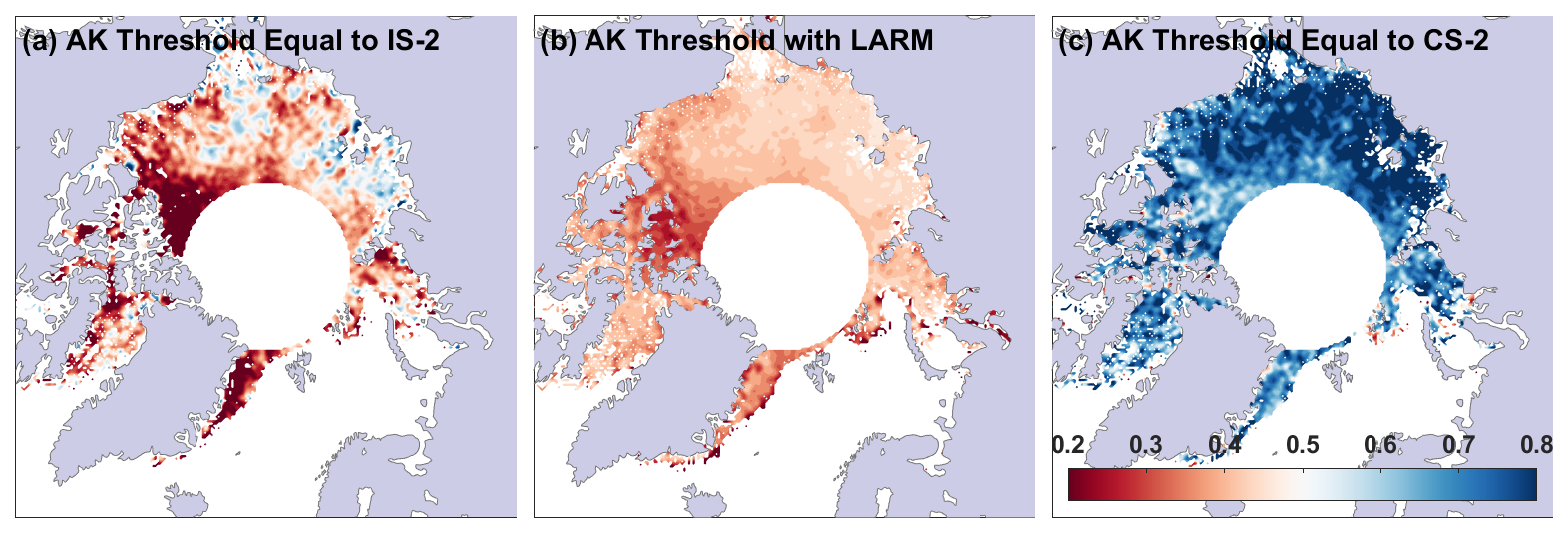
Figure 9 Fractional retracking thresholds of the first primary peak of the AltiKa waveform leading edge (a) required to match the AltiKa radar freeboard to the ICESat-2 laser freeboard, (b) obtained from the physical retracking method LARM, and (c) required to match the AltiKa radar freeboard to the CryoSat-2 radar freeboard, averaged within EASE2 25 km grid cells, in December 2018.

Previous studies have used a fixed 50 % threshold for retracking sea ice floe waveforms from AltiKa (Armitage and Ridout, 2015; Garnier et al., 2021). The grid-cell-mean AK retracking threshold that is optimized from the physical echo model with LARM is shown in Fig. 9b. There is a clear pattern with thresholds around 30 % in the MYI zone north of the Canadian Arctic, then a gradient towards thresholds of 45 % over younger FYI areas, reflecting variations in roughness (Fig. 1b). Surface-based radar studies have discovered that a significant portion of the Ka-band signal at nadir returns from the snow–ice interface, compared to the typical assumptions of satellite-based Ka-band sea ice altimetry (Stroeve et al., 2020; Nandan et al., 2023; Willatt et al., 2023). If backscatter from the snow–ice interface dominated the satellite nadir Ka-band return too, such that the AltiKa echo leading edge mainly represented the illumination of the snow–ice interface, then the floe waveforms from December 2018 would need to be retracked at the thresholds shown in Fig. 9c, i.e., at 60 %–90 %. The thresholds from LARM are much closer to those best matching IS2 than CS2, indicating that the dominant backscattering elevation is well above the snow–ice interface. However, for a perfect match to IS2 (and what we can assume is a more reliable measurement of the air–snow interface elevation Kwok et al., 2019a), the AK thresholds should look like Fig. 9a, i.e., around 20 % over the roughest sea ice areas and >50 % in areas of new ice formation where floes are smooth and specular. The spread of thresholds in Fig. 9a is wider than estimated from the LARM algorithm.

Figure 10 shows a comparison between estimates for the Ku-band radar freeboard and Ka-band radar or laser freeboard obtained from OIB and IceBird airborne reference data, and coincident freeboard observations from CryoSat-2 (light purple), AltiKa (light green), and ICESat-2 (blue), at a scale of 25 km, in April 2019. These are the same reference datasets used for the snow depth comparison in Sect. 4.4. Each satellite–airborne comparison shows some scatter, with the CryoSat-2 observations only having a correlation of 0.59 with the reference data. The correlation with the ICESat-2 observations is higher at 0.85, and the laser altimeter accurately captures grid cells with thicker freeboard from 70–90 cm in the reference data. There are fewer grid cells with reference data at latitudes <81.5° N to evaluate AltiKa, but the satellite radar altimeter also captures thinner freeboards ∼20–30 cm and thicker freeboards >70 cm, with a relatively higher correlation of 0.86 with the OIB laser freeboards. The distributions of the satellite freeboards match closely to the reference data but are typically narrower (Fig. 10b). This reflects the truncation of the true freeboard distribution in the satellite measurements, where, for instance, the kilometer scale of the radar footprint or interpolation of the SSHA over tens of kilometers makes the measurement tend more towards the modal than the mean freeboard at these scales (Ricker et al., 2014; Landy et al., 2020; Belter et al., 2020). This is also one of the main reasons why the slopes of the freeboard (Fig. 10a) and snow depth comparisons (Fig. 8) are $<\mathrm{1}.$

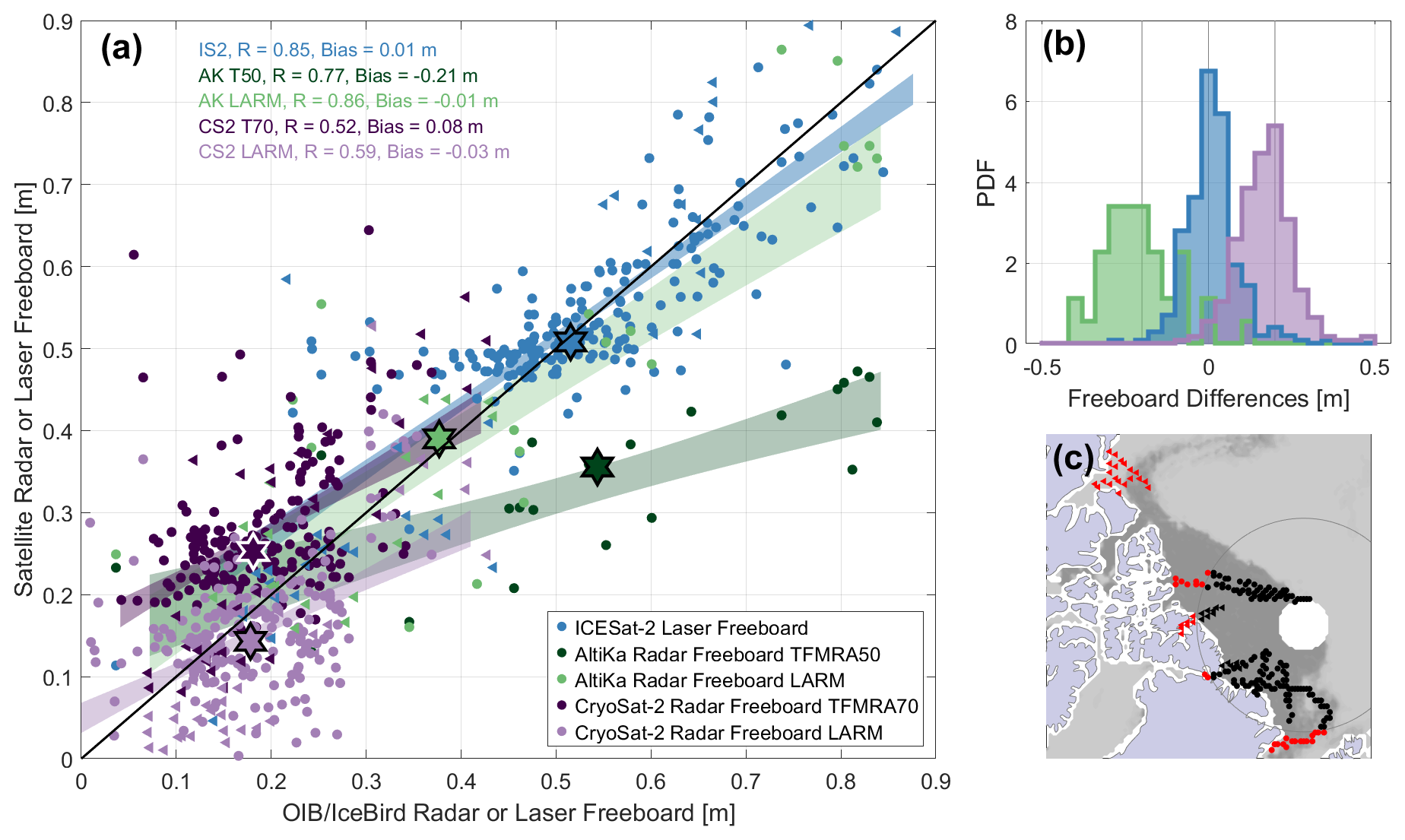
Figure 10 Comparison between satellite Ku-band, Ka-band, and laser freeboards and Ku-band and laser freeboards estimated from airborne data collected by OIB (circles) and IceBird (triangles) in April 2019. (a) Scatterplot of satellite and airborne observations resampled to the same EASE2 grid, with the median of each cluster shown by a hexagram and the 66 % confidence interval on the best-fit line through samples shown by the filled envelopes. (b) Distributions of the differences between OIB- and IceBird-estimated Ku-band radar and measured laser freeboards with corresponding paired satellite freeboards from IS2 (blue), AK LARM (green), and CS2 LARM (purple). Note that the AK distribution has been offset by −0.2 m and that the CS2 distribution has been offset by +0.2 m, highlighted by the gray lines, for visual clarity. (c) Map of the sea ice type from OSI-403-d, with FYI represented by lighter gray and MYI represented by darker gray, overlaid with the locations of corresponding airborne and satellite observations above (black) and below (red) the maximum latitude of AltiKa at 81.5° N.

The major impact of the radar waveform retracking algorithm on the ice freeboard retrieval is illustrated in Fig. 10a. In dark green and dark purple, respectively, are the same satellite–airborne comparisons but with AltiKa ice floe observations retracked with the threshold first-maximum retracking algorithm (TFMRA) at 50 % amplitude on the waveform leading edge and with CryoSat-2 floe observations retracked with TFMRA at 70 % amplitude, as described in Armitage and Ridout (2015). The radar freeboards shown for each sensor are derived with the methods described in Armitage and Ridout (2015) and Lawrence et al. (2018). With TFMRA retracking, the CryoSat-2 radar freeboards overestimate the reference data by ∼10 cm, especially over thinner ice with freeboards <25 cm. A similar positive bias, summarized by the dark-purple hexagram, was found by Lawrence et al. (2018). This freeboard bias could be a geophysical effect, as previously suggested, i.e., attenuation of the Ku-band signal in brine-wetted snow (King et al., 2015; Nandan et al., 2017; Rösel et al., 2021) or volume and internal interface scattering over snow on MYI (Ricker et al., 2015). Our analysis here shows it could alternatively be a processing effect, i.e., through the choice of retracker or another processing step in the freeboard calculation. The correlation between CryoSat-2 TFMRA and reference freeboards is 0.52, and the slopes of the CryoSat-2 fits with different retrackers are similar, so the bias is the key difference. With TFMRA, the AltiKa radar freeboards have a correlation of 0.77 with the reference freeboards and underestimate the reference data, with the bias also increasing for thicker ice (dark green in Fig. 8a). A significant negative bias, summarized by the dark-green hexagram, was found by Lawrence et al. (2018), who corrected AltiKa (and CryoSat-2) freeboards for the detected biases with calibration functions based on radar waveform pulse peakiness. A retracking threshold of 50 % produces a relatively similar result to ICESat-2 over thinner FYI floes (Fig. 9a), but the threshold needs to be <30 % to accurately measure the air–snow interface elevation over thicker MYI floes (Fig. 9a and b). This variable bias could be a geophysical effect, as previously suggested, caused by significant penetration of the Ka-band signal into snow (Armitage and Ridout, 2015; Stroeve et al., 2020), or it could, at least partly, be a processing effect of the choice of retracking algorithm and influence of surface roughness on the optimal retracking threshold (Figs. 1b and 9a) (Lawrence et al., 2018).

5.2 Physical mechanisms behind observed radar scattering biases

It is clear from Figs. 5 and 9b that biases remain in the AltiKa radar freeboards, despite improvements that can be made by retracking with a physical model for the radar scattering surface. The assumptions of the physical model, for instance, of a single dominant scattering interface, may oversimplify the interactions of the radar with snow and sea ice (Kurtz et al., 2014; Landy et al., 2019). Another possibility is that the large-scale sea ice surface topography (σ) is not accurately accounted for in the AltiKa scattering model. To explore this, we calculate the mean height differences between AltiKa and ICESat-2 freeboards as a function of the binned AK σ (Fig. 11a), obtained from the model inversion (as described in Sect. 3.3), and backscatter coefficient (Fig. 11b), as well as the binned IS2 σ (Fig. 11c), across the full data record October–April 2018–2023. This is done separately for 0.1 m intervals of the AK radar or IS2 laser freeboard from 0–0.1 up to 0.6–0.7 m. For AK freeboards up to 0.4 m (covering 91 % of grid cells across the record), the AK-IS2 freeboard bias is approximately independent of the AK surface topography, although AK freeboards <20 cm consistently underestimate those from IS2 (Fig. 11a). For AK freeboard >0.4 m, the AK-IS2 freeboard bias depends on surface topography, with AK overestimating IS2 by as much as 40 cm when the AK surface topography is very smooth but only showing a small bias when the AK topography is rougher. These findings are consistent when the bias is analyzed as a function of IS2 freeboard and surface topography (Fig. 11c), suggesting that the impact of snow surface roughness on the AK retracking point (i.e., Fig. 1b) is modeled reasonably well, except in the 3 % of cases when AK freeboard is >0.4 m but σ is <0.2 m. The high variability in the bias for the roughest IS2 surface topography (Fig. 11c) is caused by limited data: only 2 % of IS2 σ in the full record is >0.35 m.

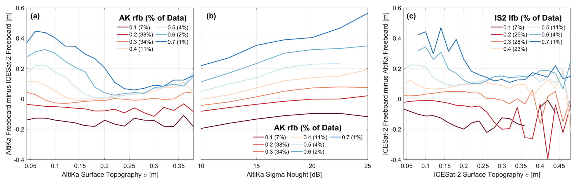
Figure 11 Height differences between coincident gridded radar freeboards from AltiKa and laser freeboards from ICESat-2 as a function of (a) the AltiKa radar scattering surface topography (σ_AK), (b) the AltiKa backscatter coefficient (sigma nought), and (c) the ICESat-2 surface topography (σ_IS2) over the period 2018–2023. In panels (a) and (b), separate lines are shown for 10 cm intervals of the AltiKa radar freeboard, and, in panel (c), separate lines are shown for 10 cm intervals of the ICESat-2 laser freeboard up to the value given in the legend. Note the percentages of the data making up each curve in the legends.

The bias between AltiKa and ICESat-2 is always positively sloped for increasing AK backscatter, with a relatively similar gradient between AK freeboard increments. If our assumption of a single dominant scattering surface, i.e., the air–snow interface, was incorrect, and the snow–ice interface and/or snow volume scattering were regularly acting to broaden the leading edge of the AK waveform producing an overestimated AK σ, we would expect the AK-IS2 freeboard bias to increase for higher AK σ. In this case, overestimated AK σ would be a strong proxy for over-penetration of the Ka-band radar. Instead, we observe that the bias is largest when there is a strong AK reflection, i.e., high sigma nought (Fig. 11b), and smoother AK or IS2 σ (Fig. 11a). In this scenario (blue lines, representing only ∼5 % of grid cells across the full record), AK and IS2 σ are totally uncorrelated (r=0.07), so the two sensors are likely to be measuring different backscattering surfaces. For the contrasting scenario, where AK underestimates IS2 (red lines, representing 63 % of valid grid cells), the curves are flat, so AK σ is unlikely to be a proxy for radar penetration (Fig. 11a). However, AK freeboard increasingly underestimates IS2 freeboard as the AK backscatter coefficient declines (Fig. 11b). This suggests that snow volume scattering (lower sigma nought) may increasingly dominate the returning Ka-band echoes vs. surface scattering/reflection (higher sigma nought), as AK increasingly underestimates IS2 freeboard.

Figure 12 shows the derived snow depth difference for KuLa (a) and KuKa (b) between January–April 2019. On average, 8.9 cm of new snow is estimated to have accumulated within the marked area over this period in the KuLa product, whereas only 3.2 cm is estimated to have accumulated in the KuKa product. Over the same period, the CS2 large-scale sea ice surface roughness (σ, derived from LARM) shows a marked increase of 5.9 cm in the same area (Fig. 12c). This is typical of the seasonal roughening of FYI in response to ice deformation (Babb et al., 2020). However, it may also partly be caused by the new snowfall from unusually intense winter storms (Kwok et al., 2020) changing the scattering response of the Ku-band signal so that significant backscatter is sourced from both the air–snow interface and the snow–ice interface (e.g., Nab et al., 2023), producing an echo with a leading edge including significant contributions from both interfaces (de Rijke-Thomas et al., 2023). Sea ice deformation and increased air–snow scattering can each cause the radar backscattering response to “spread” over a wider height distribution within the footprint (Landy et al., 2019) and reduce the total backscatter, which indeed drops by 2.6 dB on average (Fig. 12d).

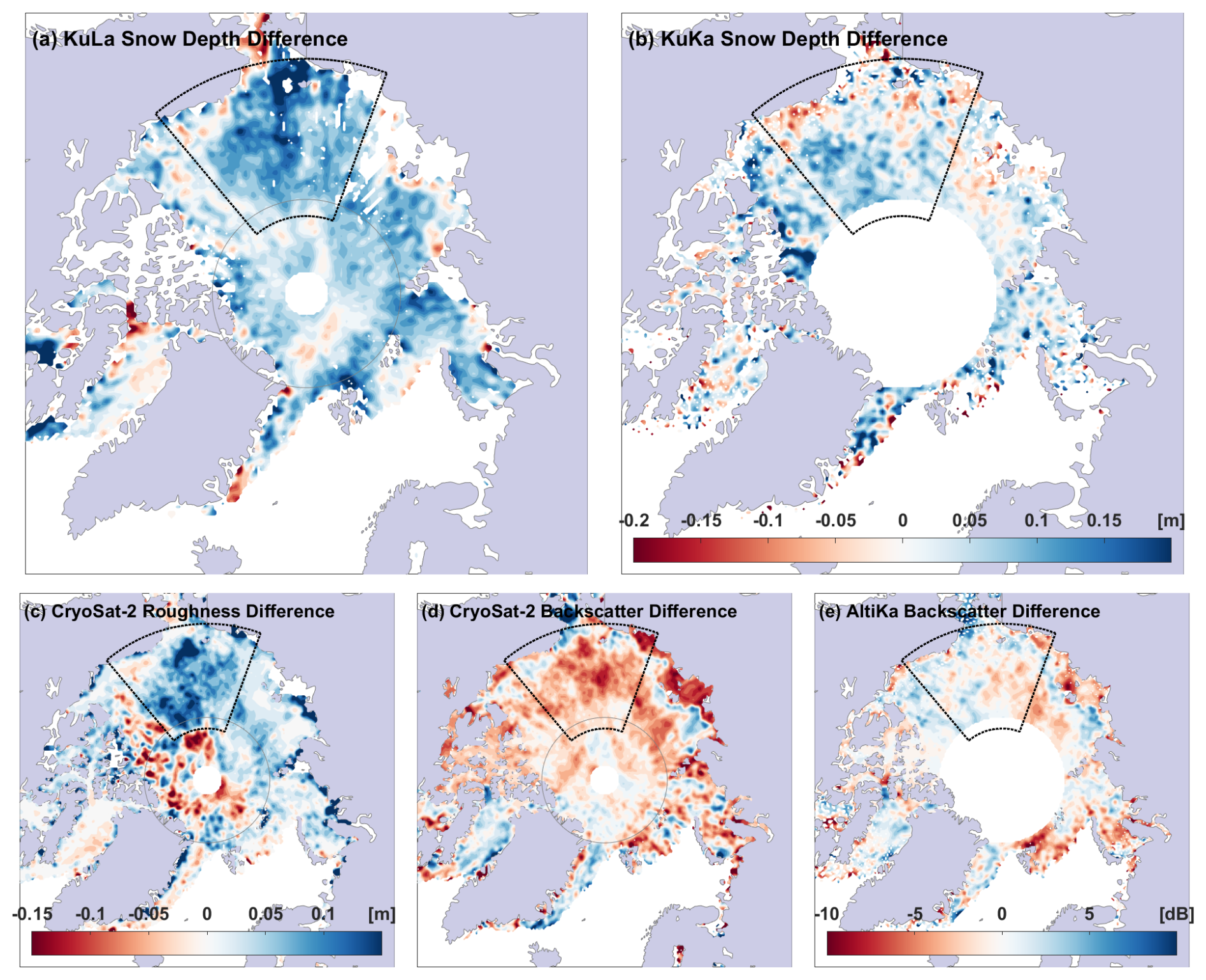
Figure 12 (a) KuLa and (b) KuKa snow depth differences (m) between January–April 2019, when a significant amount of new snow is likely to have accumulated on sea ice in the Beaufort, Chukchi, and East Siberian seas. Also shown are the concurrent changes in CryoSat-2 (c) sea ice surface roughness σ (m) (derived from LARM), (d) radar backscatter (dB), and (e) AltiKa radar backscatter (dB). The gray circles show the limit in coverage for AltiKa, and the dotted black ones mark the approximate area of rapid snow accumulation between January–April.

In contrast, the AK backscatter barely changes, with an average decrease of only 0.1 dB between January–April (Fig. 12e). Although the AK radar freeboard increases by 7.3 cm between January–April, this is around half the IS2 laser freeboard increase (14.8 cm), and there is no obvious response in the Ka-band backscatter. This suggests that the AK Ka-band signal may only respond weakly to the rapid accumulation of new snow. The Mie scattering coefficient of dry snow at the Ka band approximately halves when the snow density reduces from 350 to 175 kg m⁻³ (Long and Ulaby, 2015) (the Mie scattering coefficient quantifies the scattering of incident EM radiation by particles of similar diameter to the wavelength). The impact of AK backscatter change on the retracked height has also been recorded as only 5 cm dB⁻¹ over the Antarctic Ice Sheet (Rémy et al., 2015). Therefore, a lack of backscatter change in Fig. 12e suggests the radar remains most sensitive to surface and volume scattering from snow accumulated earlier in the season, which is deeper in the snowpack by April, and the increase in AK freeboard is mainly due to the ice freeboard thickening rather than new snow accumulation too.

5.3 Snow accumulation over newly formed sea ice

The basin-wide patterns, seasonal evolution, and validation results of the KuLa snow depths (Fig. 8) support the routine operational use of snow depth estimates from CryoSat-2 and ICESat-2. A further useful check on the consistency between these two sensors is to intercompare the radar and laser freeboards over areas of newly formed sea ice, where we would expect the freeboards – in the absence of significant snow – to be very similar. To explore this idea, we defined grid cells with new sea ice where new FYI appeared, on any given day between October–December 2018–2022, from the 10 km resolution OSISAF OSI-403-d Global Sea Ice Type product (Aaboe et al., 2021). In some cases, these grid cells will represent FYI advected from an adjacent grid cell, but, during the early ice growth period from October to December, this normally represents new FYI formation exceeding the product's minimum 30 % sea ice concentration (SIC) threshold. We then identified any of these “new ice” grid cells that were crossed by CS2 and IS2, within a 5 d period centered on the date of new ice formation and 12.5 km search radius (we decided to exclude AltiKa observations, given the limited number of occasions where all three sensors coincide within a short time window). We used L2 along-track CS2 radar freeboards from LARM and the daily gridded IS2 laser freeboards from ATL20.

The spread of valid “new ice” grid cells is shown in Fig. 13c. As expected, they are confined to typical areas of new sea ice formation in the Arctic fall, for instance, in the Beaufort, Chukchi, and Siberian Shelf seas (which we call the “Pacific Sector” here, marked in blue) and in the Greenland, Barents, and Kara seas and Baffin Bay (which we call the “Atlantic Sector” here, marked in red). There are clear differences in the derived freeboard and snow depth distributions, between these two sectors, across the 5-year study period. The CS2 radar freeboard distribution has a primary peak at 1.2 cm and a secondary peak at 6.9 cm in the Pacific Sector (Fig. 13a). The IS2 laser freeboard distribution has a similar shape, with a primary peak at 7.5 cm and a secondary peak at 11 cm. The limited number of IS2 freeboards in ATL20 thinner than 3 cm may be caused by the application of a 50 % SIC filter and negative freeboards being set to zero in ATL10, rather than a true absence of the thinnest ice. Filtering out dark leads now also reduces the prevalence of very thin IS2 freeboards (Kwok et al., 2021). The small offset in freeboards in the Pacific Sector produces derived snow depths with a mean of only 3.5 cm (Fig. 13d), showing that CS2 and IS2 are measuring approximately the same backscattering surface over sea ice in the absence of significant snow. In contrast, the radar and laser freeboard distributions are well separated in the Atlantic Sector, with means of 6.6 and 25.9 cm, respectively (Fig. 13b). There is a general pattern with thicker derived snow depths in the Barents Sea, around Svalbard, transitioning eastwards to thinner snow depths in the Kara Sea (Fig. 13c). The mean snow depth for new sea ice, within 5 d of formation, is 14.9 cm in the Atlantic Sector. These results support previous studies that suggest frequent intense cyclones (polar vortices) deposit considerable snow onto sea ice forming in the Barents Sea, soon after the date of formation (Merkouriadi et al., 2017; Graham et al., 2019). The large spread (10.2 cm standard deviation) in snow depths on new ice in the Atlantic Sector (Fig. 13d) also suggests that these heavy fall snowfall conditions are variable between years. On the other hand, the cyclone intensity is much lower in the Pacific Sector (Webster et al., 2019), leading to consistently lower rates of snow deposition on newly forming ice.

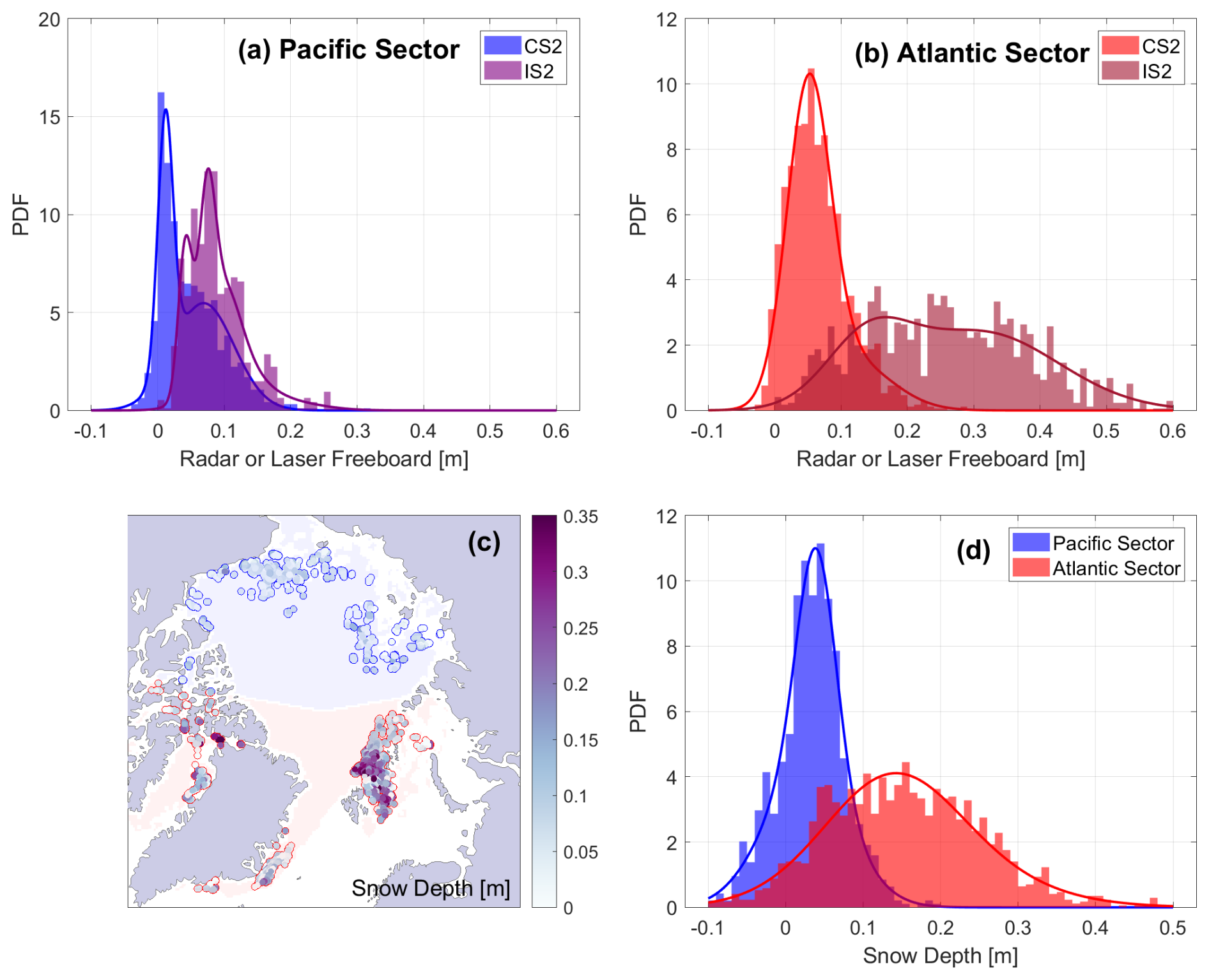
Figure 13 Estimated fresh snow depth on newly formed sea ice between 2018–2022, including CryoSat-2 and ICESat-2 freeboards in locations of newly formed ice, within the Pacific (a) and Atlantic (b) sectors of the Arctic, snow depth in locations of newly formed ice with coinciding observations from the two sensors (c), and derived snow depth distributions in the two sectors (blue = Pacific; red = Atlantic) (d). The distributions are fit with Gaussian mixture models.

5.4 Implications for CRISTAL

Although there are similarities between the radar and laser freeboards obtained by coincident Arctic observations from CryoSat-2, AltiKa, and ICESat-2, it is not straightforward how these findings will translate to the measurements expected from CRISTAL. For instance, the LRM observations from AltiKa are strongly sensitive to surface roughness, at scales up to the beam-limited footprint of the radar (∼8 km) (Guerreiro et al., 2017), whereas the delay-Doppler SAR-mode Ka-band observations from CRISTAL should be much less sensitive to roughness (Wingham et al., 2006). To investigate the potential effects of different snow properties and surface roughness on CRISTAL observations, here we use the results obtained in Sect. 4.1 and 4.2 as the basis for physically constrained simulations of the CRISTAL dual-frequency altimeter in delay-Doppler SAR mode (see sensor parameters in Table A1). In contrast to the approach described in Sect. 3.2, here we model the full backscattering response of the snow cover and sea ice, for the chosen month of April 2019, using (i) the KuLa product for the snow depth, (ii) the CS2 σ estimate as the large-scale roughness of the snow–ice interface topography, (iii) the IS2 σ estimate obtained by Duncan and Farrell (2022) as the large-scale roughness of the air–snow interface topography, and (iv) the CS2 s_rms estimate as the radar-scale roughness of both snow–ice and air–snow interfaces. Volume scattering and extinction in the snowpack are modeled with a Mie scattering scheme depending on snow density, grain radius, and temperature, as described in Landy et al. (2019). To account for variability in snow density and grain radius, we use all MicroCT observations (N=2846) collected in the month of April during the MOSAiC field campaign (Macfarlane et al., 2023).

Example Ku- and Ka-band waveforms are modeled for each 25 km grid cell of the April 2019 data (i.e., Fig. 5) as the average of 10 echoes simulated with different random realizations of the sea ice topography σ and random draws from the MOSAiC snow density and grain radius distributions. FBEM is currently only set up to simulate a single snow layer with a simplified volume scattering scheme that neglects the dense media effects (Tsang et al., 2007), underestimates the complexity of the typical multi-layered snowpack on Arctic sea ice (Macfarlane et al., 2023), and potentially reduces the impact of, for example, volume scattering from relatively large brine-wetted snow grains in the basal depth hoar layer (e.g., Nandan et al., 2017). Using the same s_rms value for both interfaces also underestimates the potential for one interface with smoother radar-scale roughness to dominate the total backscatter over the other. However, these simulation results are presented as a first approximation of snow and sea ice echoes that might be expected from CRISTAL. Each simulation includes separate component echoes for the snow surface, snow volume, and sea ice surface scattering contributions (Fig. 14a and b). For the Ku-band echo, we retrack the total waveform using the threshold determined from only the sea ice surface echo, i.e., following the necessary assumption taken in Sect. 3.1 as if we did not have snow information available for the simulation. This allows us to estimate the bias in the retracked height of the snow–ice interface, as a fraction of the snow depth, taking into account snow effects on Ku-band scattering (Fig. 14a and d). Similarly, for the Ka-band echo, we retrack the total waveform using the threshold determined from only the snow surface echo, allowing us to estimate the bias in the retracked height of the air–snow interface, as a fraction of the snow depth, taking into account Ka-band scattering effects from deeper in the snowpack and potentially from the sea ice surface too (e.g., Willatt et al., 2023) (Fig. 14b and d).

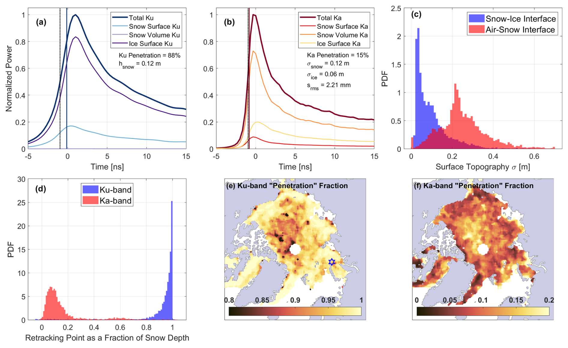
Figure 14 Simulated Ku- and Ka-band waveform returns from snow-covered sea ice, based on snow and sea ice geophysical properties estimated in April 2019, for CRISTAL in delay-Doppler SAR mode. Panels (a) and (b) show Ku- and Ka-band component echoes simulated for the grid cell to the northeast of Novaya Zemlya, highlighted with a blue star in panel (e). The five key parameters listed in panels (a) and (b) are applicable to both the Ku- and Ka-band simulations. The air–snow interface is identified by the dotted black line, the snow–ice interface is identified by zero time, and the retracking points of the waveforms are identified in blue and red, as described in the text. Panel (c) shows the pan-Arctic distributions of gridded snow–ice (σ_ice) and air–snow interface topography (σ_snow) for the month, as obtained from CS2 and IS2, respectively. Panel (d) shows distributions of the retracking points of Ku- and Ka-band waveforms, as fractions of the snow depth, for all grid cells in the month. Panels (e) and (f) show geographic variations in the “penetration” fraction of the snow depth, where 0 is the retracking point at the air–snow interface and 1 is the retracking point at the snow–ice interface.

For the Ku-band returns, the total echoes are typically dominated by the ice surface scattering component (e.g., Fig. 14a). This produces a relatively low bias in the retracking point owing to snow surface and volume scattering effects on the waveform leading edge. The retracked “snow–ice interface” height is located at a median 3 % of the relative depth of the snowpack above the true snow–ice interface; however, for 1/10 of the simulations, the retracked interface is biased >20 % of the snow depth above the true ice surface (Fig. 14d). Simulations exhibiting a larger bias are typically found in areas of rough MYI (Fig. 14e), where the CS2 σ and s_rms are larger, producing a relatively weaker radar reflection from the snow–ice interface. This enables volume scattering from snow grains to attenuate the signal and the snow surface reflection to have a larger influence on the waveform leading edge as shown by Kwok (2014) and de Rijke-Thomas et al. (2023) for airborne Ku-band radar data. At a pan-Arctic scale, the ice surface echo tends to dominate the Ku-band waveform because the slope distribution of the snow–ice interface is significantly smoother than the air–snow interface (Fig. 14c). This is backed up by airborne observations, which consistently measured a smoother snow–ice than air–snow interface topography (8 cm mean difference) for the same sea ice (Landy et al., 2020). Over FYI, the relatively smooth sea ice surface generally produces a strong radar reflection (de Rijke-Thomas et al., 2023) and therefore low bias in the retracking point (Fig. 14e).

For the Ka-band returns, the total echoes typically include a strong contribution from snow volume scattering (e.g., Fig. 14b). This has been suggested previously for Ka-band returns from snow (Rémy et al., 2015; Guerreiro et al., 2017; Larue et al., 2021); for instance, Adodo et al. (2018) found that the seasonal cycle of Ka-band backscatter over the Antarctic Ice Sheet is governed by the volume echo. However, in the Ka-band waveform simulations of Meloche et al. (2024), the volume backscatter was only found to dominate the total echo when the interface roughness exceeded 3–4 mm. Here, the bias on the retracking point for the air–snow interface is larger than for the snow–ice interface with Ku-band echoes because a weak reflection from the air–snow interface and volume scattering from deeper within the snowpack, or a strong reflection from the snow–ice interface, shifts the waveform leading edge to later range bins. The retracked “air–snow interface” height is located at a median 10 % of the relative depth of the snowpack below the true air–snow interface; however, for 17 % of the simulations, the retracked interface is biased >20 % of the snow depth below the true snow surface (Fig. 14d). The bias is larger when the snow surface scattering contribution is smaller and the volume scattering coefficient is lower (e.g., Rémy et al., 2015), such that backscatter increases less rapidly as the pulse propagates into the snow pack. When the CS2 σ is low relative to the IS2 σ (Fig. 14c), and the snow density and grain size are relatively low, the specular radar reflection from the snow–ice interface can be the strongest contributor to the waveform leading edge, and the height of the air–snow interface is underestimated by >50 % of the snow depth. In this scenario, the snow–ice interface can occasionally be seen as a secondary peak in the echo, mirroring results from surface-based radar studies at the Ka-band (Stroeve et al., 2020; Nandan et al., 2023; Willatt et al., 2023).

6 Conclusions

Our study supports the theoretical basis for along-track snow depth on sea ice retrieval from the dual-frequency observations of the CRISTAL mission. The magnitudes of the radar freeboards obtained from the Ku-band SAR mode CryoSat-2 data are significantly thinner than those obtained from the Ka-band LRM mode AltiKa data. However, the freeboards derived from CryoSat-2 and AltiKa observations can vary significantly depending on the techniques used to process them, particularly in the waveform retracking step. The roughness of the radar scattering surface has a major impact on the threshold that should be used to retrack altimeter waveforms, potentially introducing biases of tens of centimeters into the relative height measured over sea ice floes. Care must therefore be taken in the interpretation of radar freeboards to disentangle the sources of bias coming from geophysical factors, such as complex radar scattering over layered snow and sea ice vs. those from processing choices, with respect to some reference “truth”. Retracking thresholds of 20 %–30 % over MYI and >50 % over new sea ice are required to match AltiKa radar freeboards to ICESat-2 snow freeboards, covering a wider spread of thresholds than our physical retracker LARM uses to account for surface roughness. This implies that the roughness of the radar scattering surface is not the only factor affecting Ka-band radar freeboards in LRM altimetry.

There are strong similarities in the Arctic Basin-wide patterns of freeboard obtained from CryoSat-2, AltiKa, and ICESat-2, albeit with different magnitudes. Ka-band LRM freeboards can diverge from laser altimeter freeboards when the radar is not sensitive to scattering from newly deposited snow or when the impacts of surface roughness are not properly accounted for in the freeboard processing. Snow depths estimated from the difference between Ku-band and laser freeboards show accumulation rates of 1.9 cm month⁻¹ over FYI and 1.5 cm month⁻¹ over MYI; however, the accumulation rates for snow depths estimated from Ka- and Ku-band freeboards were only one-third of the KuLa accumulation rates at 0.5 cm month⁻¹. The interannual variability in the KuLa snow depths measured over the 5-year record is 1 order of magnitude lower than estimated from the reanalysis-based snow model accumulation scheme SnowModel-LG. Filtering only the cases for which CryoSat-2 and ICESat-2 freeboards observe the same area of newly forming sea ice, in the MIZ, shows that Pacific Sector snow depths are 3.5 cm within the first 5 d of ice formation, whereas Atlantic Sector depths are 3 times thicker over the same time span. Despite this rapid initial accumulation, Atlantic Sector snow depths are not considerably thicker than Pacific Sector depths by the end of the accumulation season in spring.

Model simulations of CRISTAL, in its anticipated sea ice sensing mode, suggest that, in spring, the altimeter will track a median Ka-band elevation 10 % below the air–snow interface and a median Ku-band elevation 3 % above the snow–ice interface. However, in 17 % and 10 % of cases, respectively, the retracked elevation is off by more than 20 %. Our derived KuKa snow depths have an RMSE of 8.9 cm vs. OIB and IceBird airborne observations and an RMSE of 10.4 cm vs. the KuLa snow depths (across all 35 measured winter months from 2018–2023). The CRISTAL mission is required to measure sea ice freeboard, snow depth, and ice thickness with uncertainties lower than or equal to 3, 5, and 15 cm, respectively, at a 25 km length scale equivalent to our gridded and airborne and satellite comparisons (Kern et al., 2020). An 8–10 cm snow depth uncertainty introduces 17–29 cm sea ice thickness uncertainty (Ricker et al., 2014), even if the Ku-band radar freeboard is measured with absolute certainty. Consequently, the uncertainties of KuKa snow depths obtained from CryoSat-2 and AltiKa are currently too high to meet the mission requirements for snow depth and ice thickness uncertainties. However, the novelty of approximately coincident along-track, Doppler-sharpened Ku- and Ka-band footprints may enable the snow depth uncertainties estimated from CRISTAL to be reduced by the 5–6 cm required to meet the mission goals.

Analyzing coincident freeboards and surface roughness observations from three different altimeters, and using these results to constrain simulations of Ku-/Ka-band SAR-mode radar echoes over snow-covered sea ice, offers some lessons in advance of the CRISTAL launch. For instance, it would be valuable to study, in more depth, (i) the covariance of the snow and sea ice surface topography at scales of 1–1000 m and its impact on near-nadir radar reflection, (ii) bounds on millimeter–centimeter radar-scale roughness of snow and ice interfaces and the external factors controlling these roughness variations in time and space, (iii) the evolution of the satellite Ku- and Ka-band radar return from the same snow and sea ice (e.g., landfast ice) over time to observe the effects of changing snow properties (depth, grain size, layering, dielectrics) on the backscatter and waveform shape, and (iv) auxiliary remote sensing observations or model output to support the interpretation of CRISTAL multi-frequency waveforms; for example, having the anticipated snowpack properties or an estimate for the multi-scale roughness of a radar observation would enable the application of smart freeboard bias corrections. All these recommendations apply equally to the Southern Ocean and the Arctic Ocean, where the snow and surface roughness properties can be quite different.

In any case, the CRISTAL observations promise to revolutionize our understanding of the topography and thickness of Arctic snow and sea ice as it continues to evolve in response to climate warming, extending the record of sea ice volume required to understand Arctic mass and energy budgets, improve seasonal ice edge forecasts, and benchmark future climate model projections.

Appendix A:  

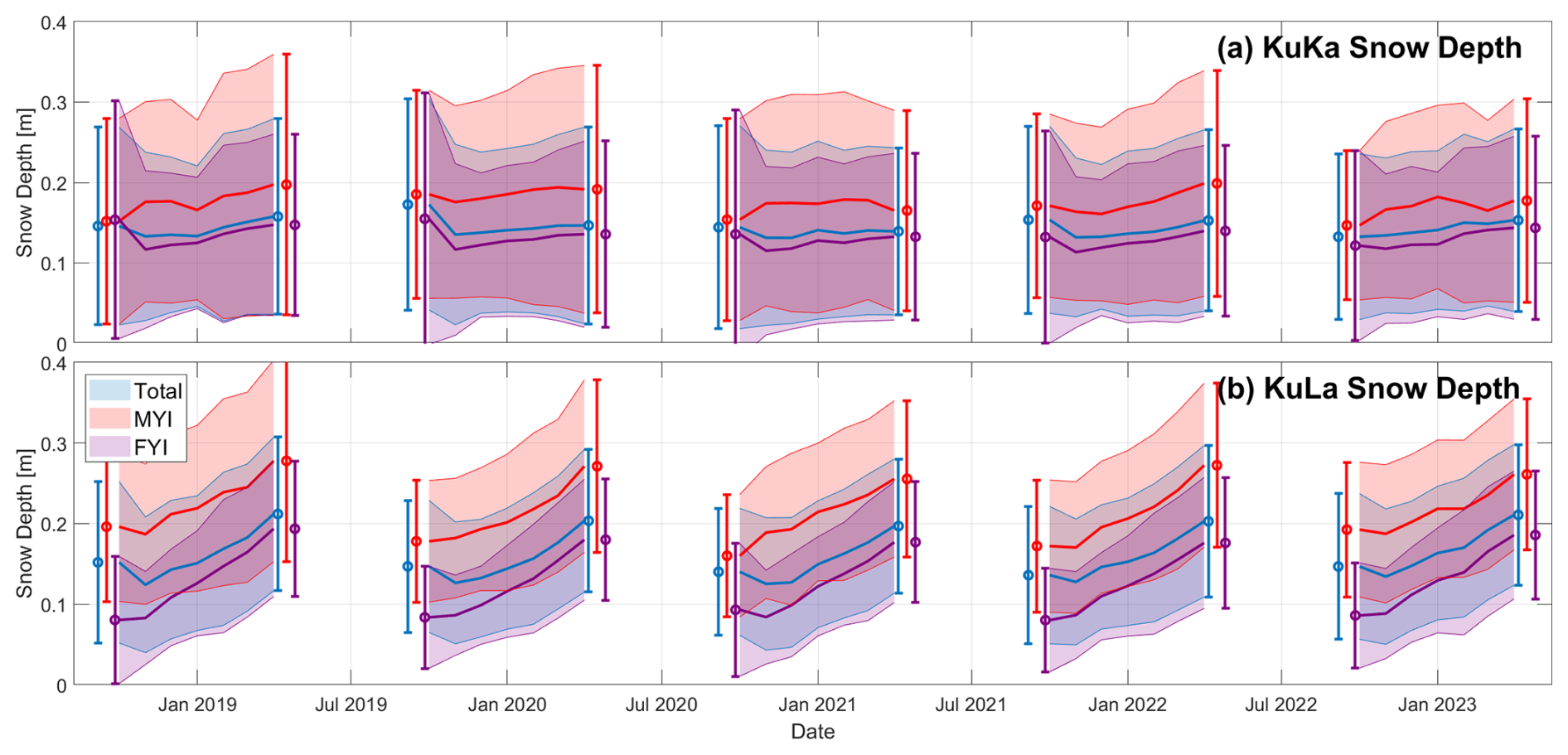
Figure A1 Copy of Fig. A1 but including KuLa snow depth estimates up to 88° N. Time series for the seasonal change in snow depth obtained from (a) KuKa radar and (b) KuLa radar and laser freeboards over the 2018–2023 sea ice growth/snow accumulation seasons. The envelopes represent ± 1 standard deviation around the mean snow depth. The points and whiskers show snow depths around the mean of 1 standard deviation at the start and end of each observation season.

Table A1 Parameters used for simulations of the Interferometric Radar altimeter for Ice and Snow (IRIS) in delay-Doppler SAR mode at Ku-band and Ka-band frequencies. Hamming weighting is applied prior to the beam-wise azimuth FFT. Other relevant sensor and target parameters not specified here are as listed in Landy et al. (2019).