In situ monitoring of seasonally frozen ground using soil freezing characteristic curve in permittivity–temperature space

Seasonally frozen ground (SFG) is a critical component of the cryosphere, yet its freezing dynamics are often oversimplified in large-scale monitoring frameworks – particularly in remote sensing (RS) and land surface modeling – through the use of binary 0 °C thresholds. This approach overlooks the physically significant “transitional” state where liquid water and ice coexist, leading to systematic errors in quantifying the timing and duration of the frozen season. To address this, we recast the Soil Freezing Characteristic Curve (SFCC) framework directly into permittivity–temperature space. By operating in dielectric space, we bypass the high uncertainty associated with soil-specific liquid water content calibrations and enable a robust categorization of soil into unfrozen, transitional, and frozen states. We fitted this model to in-situ measurements from eight monitoring networks (87 sites) across Canadian boreal forest, prairie, and tundra ecozones. Using Bayesian hierarchical partial pooling, we derived stabilized estimates of the freezing onset (T_f) and transition sharpness (b). Network-level T_f ranged from 0.15–0.44 °C, while b varied from 0.92–3.47 °C⁻¹, reflecting distinct freezing regimes. We found that the transitional state is a dominant seasonal feature at these sites, challenging binary 0 °C assumptions used in RS evaluation. In high-moisture sites characterized by thick organic insulation (e.g., within the observed eastern boreal forest networks), this state persisted for over 100 d – effectively the entire winter – despite persistent subzero air temperatures. In contrast, sites in the western boreal and prairie networks, which generally lack thick surface organic layers and have lower soil moisture, exhibited shorter but still significant transitional periods (30 and 60 d, respectively). Even in the extreme cold of the tundra network sites, the transitional phase persisted for over 40 d. These results confirm that surface insulation and soil moisture, rather than air temperature alone, govern the SFG regime at the observed locations, providing a reproducible, physically-based reference framework for the next generation of freeze–thaw products.

1 Introduction

Seasonally frozen ground (SFG), affecting most land areas above 45° N latitude (Zhang et al., 2003), is defined as a condition in which pore water turns into ice (Williams and Smith, 1989). It plays a major role in the land surface energy and water balance, impacting ecological, hydrological, and biological processes in cold regions (Ala-Aho et al., 2021; Hayashi, 2013; Ping et al., 2015; Loranty et al., 2018). By affecting hydrological partitioning, SFG regulates key processes such as infiltration, groundwater recharge, water chemistry, and runoff characteristics (Ala-Aho et al., 2021). Furthermore, SFG impacts soil respiration – the primary pathway of carbon emissions to the atmosphere – as microbial activity is largely regulated by soil temperature and liquid water availability (Davidson and Janssens, 2006; Lei et al., 2022; Nikrad et al., 2016; Arndt et al., 2023; Azizi-Rad et al., 2022; Mikan et al., 2002; Mavrovic et al., 2023). Therefore, accurately quantifying the timing, extent, and duration of SFG is critical for tracking environmental shifts and predicting changes in these vital ecosystem processes.

A common approach to monitoring SFG is the use of a simplistic temperature threshold – typically 0 °C – to distinguish between frozen and unfrozen states. However, this binary classification fails to capture the physically significant “transitional” phase where liquid water and ice coexist. This limitation is particularly prevalent in the remote sensing (RS) community; many freeze–thaw (FT) studies, ranging from foundational work (Kim et al., 2011; Zhang and Armstrong, 2001) to recent applications (Donahue et al., 2023; Taghipourjavi et al., 2024; Gao et al., 2020; Kou et al., 2017; Roy et al., 2020; Derksen et al., 2017), rely on 0 °C soil or air temperature thresholds for model training and evaluation. By neglecting the partially frozen state, these models may misrepresent the timing and duration of the frozen season. Only recently have researchers begun integrating soil moisture and temperature dynamics via the Soil Freezing Characteristic Curve (SFCC) into FT model evaluation (Rautiainen et al., 2025). The SFCC defines the relationship between liquid water content (θ_lw) and subzero temperatures (Spaans and Baker, 1996; Koopmans and Miller, 1966), offering a framework for capturing the complexities of the soil freezing process across three distinct zones: the unfrozen zone, the transitional zone, and the residual zone (Fig. 1, see Sect. S1 in the Supplement for further details).

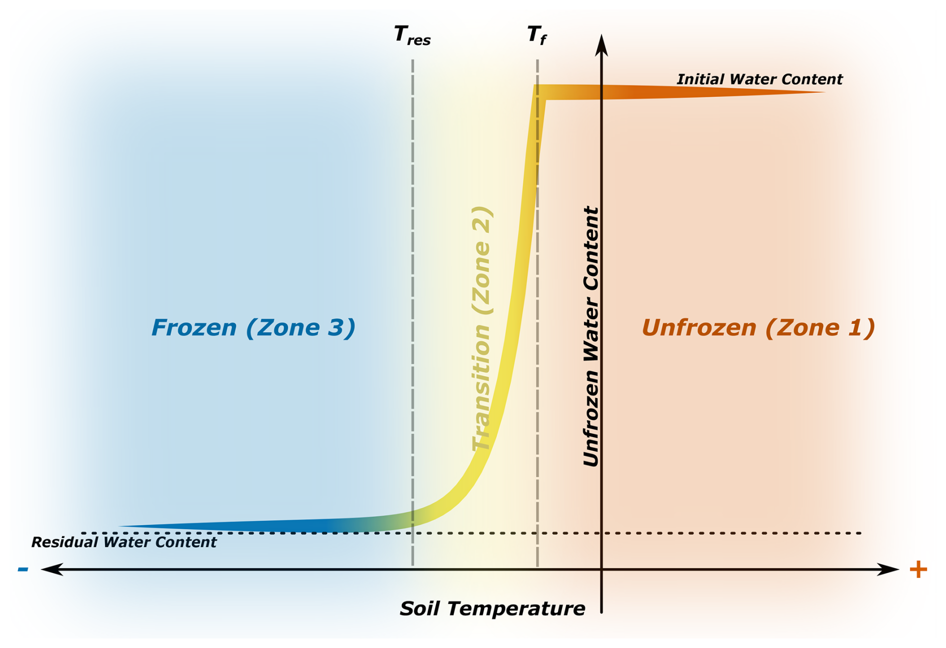
Figure 1 A typical Soil Freezing/Thawing Characteristic Curve (SFCC/STCC), adapted from Zhang et al. (2019). T_f marks the temperature at which soil begins to freeze, while T_res indicates the temperature at which the liquid water content stabilizes near the residual water content.

Dielectric-based methods are widely used to estimate θ_lw by exploiting the high permittivity contrast between liquid water (ε_lw≈80), soil minerals (ε_soil≈5), and ice (ε_ice≈3.2) (Seyfried and Murdock, 1996; Smith and Tice, 1988). However, relating bulk permittivity (ε_eff) to θ_lw in frozen soils remains challenging. Dielectric mixing models require accurate ice content estimates, which are difficult to obtain in situ, while empirical models often rely on calibrations developed for unfrozen soils that do not account for the dielectric contribution of ice (Amankwah et al., 2022; Zhou et al., 2014; Yoshikawa and Overduin, 2005). These limitations make constructing a traditional moisture-based SFCC problematic in dynamic field environments (see Sect. S2 for further details). To address this, we recast the SFCC directly into permittivity–temperature space. This demonstrates that for qualitative state classification (frozen, transitional, or unfrozen), the problematic conversion of permittivities into water content is effectively unnecessary.

Beyond air temperature, soil freezing is primarily regulated by surface cover – including snowpack, vegetation, and organic (humus) layers – as well as soil moisture (MacKinney, 1929). Collectively, surface cover acts as a thermal buffer, moderating soil–atmosphere heat exchange and reducing frost penetration (Fu et al., 2018; Zhang, 2005; Decker et al., 2003). Meanwhile, soil moisture exerts a dual control: latent heat delays freezing onset, while ice formation increases thermal conductivity, accelerating subsequent cooling (Kersten, 1949; Lei et al., 2020).

In this study, we apply the SFCC framework in permittivity–temperature space to monitor SFG across 87 sites in eight Canadian monitoring networks spanning boreal forest, prairie, and tundra ecozones. Using measurements from three sensor types (HydraProbe, TEROS12, and CS616), we derive soil freezing probabilities and investigate how freezing dynamics vary across distinct landscapes. This framework establishes a reproducible methodology to bridge the gap between in situ monitoring and the validation requirements of the RS community. Furthermore, the dataset generated through this analysis is directly applicable for the training, evaluation, and refinement of satellite-based freeze–thaw algorithms and land surface models.

2 Materials and Methods

2.1 Data Collection

2.1.1 In Situ Soil Measurements

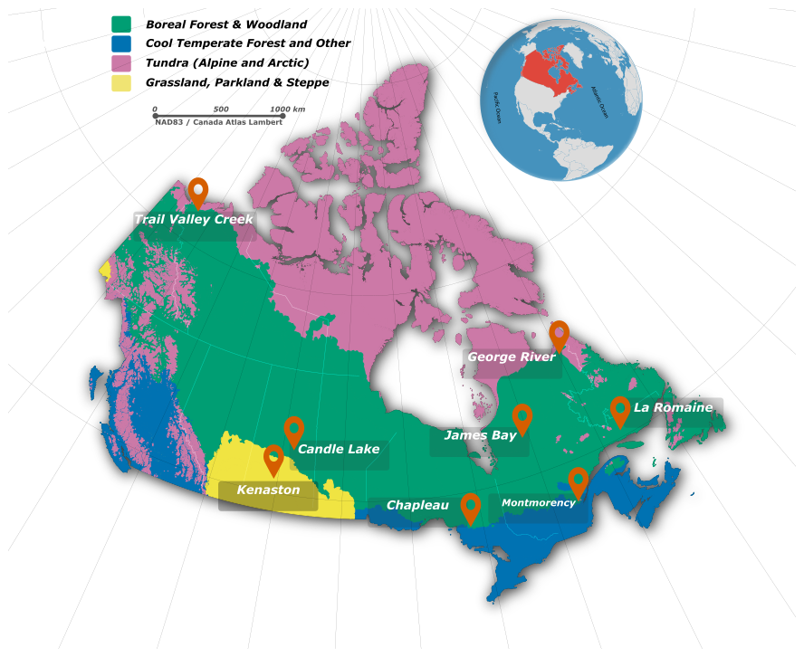
This study leverages in situ measurements of ε_eff and soil temperature to monitor the soil freezing processes. Our research spans eight networks located in diverse ecozones (Table 1 and Fig. 2), including Montmorency Forest (FM), La Romaine (LR), James Bay (BJ), Chapleau (CP) in eastern boreal forests, Candle Lake (BT) in western boreal forest, Kenaston (KN) in prairies, and Trail Valley Creek (TV) and George River (GR) in tundra. Three types of soil moisture sensors – HydraProbe (Stevens Water), TEROS12 (METER Group), and CS616 (Campbell Scientific) – were deployed based on availability across the monitoring networks. HydraProbe and TEROS12 simultaneously measure soil temperature and moisture, whereas the CS616 requires a separate soil temperature sensor (CS109SS-L) for temperature measurements. We provided an overview of these sensors, including their measurement principles and operational specifics, in Appendix A. At most sites, soil moisture probes were horizontally inserted to a depth of 5 cm, primarily within the organic layer unless it was notably thin, in which case measurements extended into the mineral layer. For the TEROS12 and HydraProbe, insertion was horizontal at this depth. In the Chapleau network, the CS616, with its 30 cm needle, was inserted at a 20° angle to integrate measurements over the top 10 cm of soil, with the midpoint depth set at 5 cm, thereby ensuring comparability with other sites (Fig. B1). Each site typically features a single sensor, except for Chapleau and Trail Valley Creek. Chapleau includes 24 CS616 sensors distributed across four 200 m×200 m plots, each representing a different forest type (Hanes et al., 2023). Since only one soil temperature sensor was available in the middle of each plot, data from multiple CS616 sensors were averaged to represent the soil conditions of that plot. At Trail Valley Creek, 12 HydraProbes were distributed across six sites (Montpetit et al., 2024), and data from each sensor were analyzed separately. Site- and sensor-specific calibration was not performed prior to installation; however, the use of manufacturer specifications and previously published validation studies provides confidence in the measurement accuracy of the deployed sensors within their expected uncertainty ranges (Seyfried and Murdock, 2004; Pardo Lara et al., 2021; Kelleners et al., 2005; Logsdon, 2009; Cominelli et al., 2024; Fragkos et al., 2024). A general quality control procedure was applied by removing physically implausible values, defined as soil temperatures outside the range of $-\mathrm{60}-\mathrm{60}\mathrm{°}\mathrm{C}$ and permittivity values outside the range of 1–90. All in situ measurements were then subjected to a standardized preprocessing workflow. Data were resampled to a uniform hourly resolution, and a continuous time index was constructed to ensure temporal consistency. Missing values were filled using linear interpolation; however, interpolated values were used solely for categorical soil state labeling and were excluded from all curve-fitting analyses to preserve the integrity of model-derived parameters. The distribution of sites within each network is strategically designed to capture the ecological diversity and maximize spatial variability, influenced by the challenging terrain and limited accessibility of the network areas. Detailed characteristics for each site – including geographic coordinates, soil textural composition (clay, sand, and silt percentages), organic content, specific soil types, elevation and stratification of soil layers – are available through an interactive map hosted in a GitHub repository (Soil-Temperature-Permittivity-Monitoring-Sites) (Salmabadi et al., 2025).

Table 1 Summary of soil moisture sensor deployment across our networks.

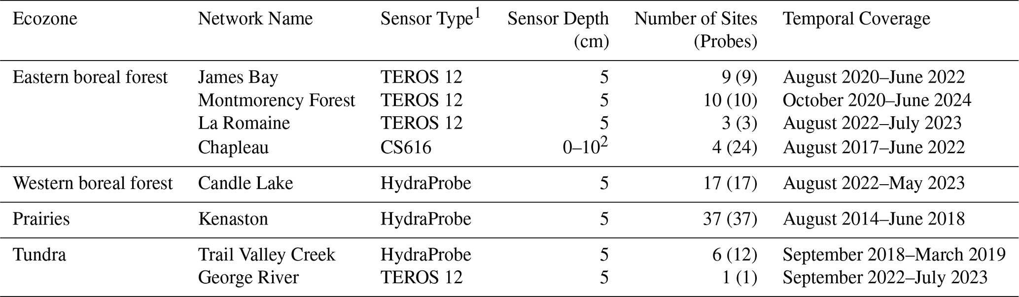
¹ All sensors include built-in soil temperature measurement, except the CS616, which requires a separate soil temperature sensor (CS109SS-L). ² The CS616 is angled at 20°, measuring the top 10 cm of soil with a midpoint at 5 cm.

Figure 2 Geographic distribution of monitoring networks across Canadian landscapes. The land cover map is adapted from Latifovic (2019).

2.1.2 Ancillary Data

Air temperature data were obtained from the ERA5-Land reanalysis developed by the European Centre for Medium-Range Weather Forecasts (ECMWF; C3S, 2018). ERA5-Land provides hourly 2 m air temperature at 0.25° spatial resolution and assimilates global observations within a physics-based numerical model to produce a consistent reanalysis extending from 1940 to the present. Snow cover data were derived from the Interactive Multisensor Snow and Ice Mapping System (IMS) produced by the U.S. National Ice Center (U. S. National Ice Center, 2004), which provides daily binary snow-cover maps for the Northern Hemisphere at 4 km resolution since 2004. The IMS product integrates multisensor satellite imagery and in situ observations. For each study site, snow-cover and air-temperature values were extracted from the corresponding IMS and ERA5-Land grid cells. Soil texture and organic carbon were obtained from the 100 m soil landscape grids of Canada (CanSIS; Geng et al., 2025). This dataset provides soil attributes at 100 m resolution using machine-learning-based predictive mapping. For this study, we extracted values specifically for the 0–5 cm depth interval at each site.

2.2 Data Preprocessing

The data preprocessing stage began by converting the raw outputs of the sensors into ε_eff for the bulk soil. This process varied depending on the sensor type, as each sensor produced different raw outputs. Detailed explanations of these sensor-specific preprocessing steps are provided in Appendix A. Next, we identified freezing and thawing cycles based on trends in soil temperature and ε_eff. A freezing cycle was defined as the period when soil temperature started decreasing and reached its minimum, while a thawing cycle extended from this minimum until temperatures rose above zero. This approach aimed to capture the main freezing and thawing events while excluding minor fluctuations, where temperatures briefly rose above or fell below zero within a narrow range, resulting in incomplete or transient freezing or thawing. Specifically, any fluctuations within ±2σ_T of 0 °C, where σ_T represents the instrument-specific temperature uncertainty, were ignored (see Appendix A for details on sensor uncertainty). If, during a freezing cycle, the soil temperature never dropped below the −σ_T threshold and ε_eff remained relatively unchanged, we classified these sites as never frozen. Although curve fitting was not feasible for these cycles due to insufficient data in Zones 2 and 3, they were retained for subsequent analysis of freeze monitoring across our networks. We assumed that the total water content in the system remained equal to the initial water content and did not change during the freezing or thawing processes (He and Dyck, 2013). We monitored ε_eff throughout both freezing and thawing cycles to validate this assumption. We interpreted significant, sudden surges in ε_eff as indicators of additional water entering the system, violating this assumption. Consequently, we excluded such cycles from further analysis. While this assumption generally held during freezing cycles, it was often invalid during thawing cycles, primarily due to snowmelt introducing substantial amounts of water into the soil. As a result, the SFCC could be reliably constructed for freezing cycles, but constructing the STCC from in situ measurements during thawing cycles was not feasible. Therefore, in this study we focused exclusively on freezing cycles, excluding thawing cycles from further analysis.

The final step in the preprocessing of in situ data involved ensuring a balanced dataset to prevent overfitting during the curve-fitting process. In practice, the distribution of data across temperature ranges was often uneven, which could bias the fitting process. We averaged ε_eff values within a 0.1°C temperature range to address this imbalance, corresponding to the sensors' temperature resolution. This approach not only compensated for the uneven distribution but also reduced noise caused by diurnal temperature fluctuations. Such fluctuations, while absent in controlled laboratory settings, were common in in situ environments.

2.3 Data Processing

2.3.1 SFCC Model

In this study, we applied the theoretical model introduced by Bai et al. to construct the SFCC, which estimates liquid water content as a function of soil temperature:

$$\begin{array}{}\text{(1)}& {\mathit{\theta }}_{\text{lw}}=\left\{\begin{array}{ll}({\mathit{\theta }}_{\text{int}}-{\mathit{\theta }}_{\text{res}}){\mathrm{e}}^{b(T_{\text{soil}}-T_{\mathrm{f}})}+{\mathit{\theta }}_{\text{res}}& \text{if }{T}_{\text{soil}}<T_{\mathrm{f}}\\ {\mathit{\theta }}_{\text{int}}& \text{if }{T}_{\text{soil}}\ge T_{\mathrm{f}}\end{array}\right.\end{array}$$

where θ_lw, θ_int, and θ_res represent the liquid, total (initial water content prior to freezing), and residual water content, respectively. T_soil is the soil temperature, T_f is the freezing onset temperature, and b controls the transition sharpness, representing the shape factor of the distribution function (°C⁻¹).

The relationship between the ε_eff and θ_lw can be physically derived using mixing models (Amankwah et al., 2022; Kelleners and Norton, 2012; Roth et al., 1990), which express effective (bulk) permittivity as a volume-weighted average of soil components:

$$\begin{array}{}\text{(2)}& {\mathit{\epsilon }}_{\text{eff}}^{\mathit{\alpha }}={\mathit{\theta }}_{\text{lw}}{\mathit{\epsilon }}_{\text{lw}}^{\mathit{\alpha }}+{\mathit{\theta }}_{\text{ice}}{\mathit{\epsilon }}_{\text{ice}}^{\mathit{\alpha }}+(n-{\mathit{\theta }}_{\text{lw}}-{\mathit{\theta }}_{\text{ice}}){\mathit{\epsilon }}_{\text{air}}^{\mathit{\alpha }}+(\mathrm{1}-n){\mathit{\epsilon }}_{\text{soil}}^{\mathit{\alpha }}\end{array}$$

where n represents the soil porosity, and ε_eff, ε_soil, ε_lw, ε_ice, and ε_air are the relative dielectric permittivities (dimensionless) of bulk soil, soil solids, liquid water, ice, and air, respectively. The parameter α depends on soil structure and composition, ranging from −1 (parallel arrangement) to 1 (series arrangement), with α≠0 (Amankwah et al., 2022). Solving for θ_lw gives:

$$\begin{array}{}\text{(3)}& {\mathit{\theta }}_{\text{lw}}={\displaystyle \frac{{\mathit{\epsilon }}_{\text{eff}}^{\mathit{\alpha }}-(\mathrm{1}-n){\mathit{\epsilon }}_{\text{soil}}^{\mathit{\alpha }}-n{\mathit{\epsilon }}_{\text{air}}^{\mathit{\alpha }}-{\mathit{\theta }}_{\text{ice}}\left({\mathit{\epsilon }}_{\text{ice}}^{\mathit{\alpha }}-{\mathit{\epsilon }}_{\text{air}}^{\mathit{\alpha }}\right)}{{\mathit{\epsilon }}_{\text{lw}}^{\mathit{\alpha }}-{\mathit{\epsilon }}_{\text{air}}^{\mathit{\alpha }}}}\end{array}$$

This equation defines the relationship between θ_lw and ε_eff, where ε_air, ε_lw, and ε_ice are known constants with minimal temperature dependence, while n, α, and ε_soil vary with soil composition and structure and are treated as unknowns. We modified the model by Bai et al. (2018) (Eq. 1) by incorporating Eq. (3) to implement the SFCC in permittivity–temperature space. The detailed solution process is presented in Appendix C. The modified equation is:

$$\begin{array}{}\text{(4)}& {\mathit{\epsilon }}_{\text{eff}}\left(T\right)=\left\{\begin{array}{ll}{\left(\left({\mathit{\epsilon }}_{\text{int}}^{\mathit{\alpha }}-{\mathit{\epsilon }}_{\text{res}}^{\mathit{\alpha }}\right){\mathrm{e}}^{b(T_{\text{soil}}-T_{\mathrm{f}})}+{\mathit{\epsilon }}_{\text{res}}^{\mathit{\alpha }}\right)}^{\frac{\mathrm{1}}{\mathit{\alpha }}}& \text{if }T<T_{\mathrm{f}}\\ {\mathit{\epsilon }}_{\text{int}}& \text{if }T\ge T_{\mathrm{f}}\end{array}\right.\end{array}$$

Here, ε_int represents the pre-freezing ε_eff, corresponding to the system's total water content, which is assumed to approximate the initial water content (He and Dyck, 2013). ε_res is the ε_eff associated with the residual water content. The parameter α, as mentioned earlier, is an exponent that depends on the soil structure and composition. In short, by incorporating a dielectric mixing model into the Bai et al.'s model, we formulated the SFCC in the permittivity–temperature space, where ε_eff is expressed as a function of soil temperature through parameters b (°C⁻¹), T_f, ε_int, and ε_res, derived via curve fitting.

2.3.2 SFCC Model Fitting and Parameter Estimation

To derive the model parameters – ε_int, ε_res, b, and T_f – and construct the SFCC, we applied a systematic data processing and curve-fitting approach tailored to our SFCC model (Eq. 4). We used non-linear least squares optimization with initial guesses and parameter bounds. The curve fitting was conducted using the curve_fit function from the SciPy library (version 1.13.1) in Python (Virtanen et al., 2020), employing the Trust Region Reflective (TRF) algorithm, which optimizes parameter values while keeping them within predefined bounds. Since the fitting is performed independently for each site and cycle, variations in absolute ε_eff values, caused by differences in probe operating frequencies – due to the frequency-dependent dielectric properties of water and bulk soil – do not affect soil state monitoring.

To ensure that the data used for model fitting primarily reflect the freezing process, we included only measurements where T_soil≤2 °C, capturing temperatures where freezing processes are actively occurring. During initial analyses, α, the exponent representing soil structure in the dielectric mixing model (Eq. 3), consistently converged to boundary values without improving model fit, indicating low sensitivity. This issue likely stems from eliminating parameter B when deriving the SFCC model from Bai et al. (2018)'s framework (Eq. C17). This reduction decreases the model's dependence on soil parameters such as porosity and soil solid permittivity, both of which influence α. To enhance model stability and interpretability, we fixed α at 0.5, a commonly used value (Pardo Lara et al., 2020; Seyfried et al., 2005). We set the lower bound of ε_res at 1, the lowest measurable probe range, and constrained the upper bound to remain below ε_int to prevent unrealistic values. The initial effective permittivity, ε_int, representing pre-freezing soil permittivity, was initialized as the mean ε_eff within ${\mathit{\sigma }}_{\mathrm{T}}\mathrm{°}\mathrm{C}\le T_{\text{soil}}\le \mathrm{2}\mathrm{°}\mathrm{C}$, where σ_T represents the instrument-specific temperature uncertainty (see Appendix A for details on sensor uncertainty). This range ensures that mainly unfrozen-state data (Zone 1) contribute to the estimate, accounting for sensor uncertainty. The bounds for ε_int were set as the observed minimum and maximum ε_eff within this range. The exponential constant b, which controls the transition from ε_int to ε_res, was initialized at 1.0, with a lower bound of 0.1 to prevent overly gradual transitions and no upper bound. For the T_f, we allowed values up to +1°C to accommodate known measurement biases and sensor discrepancies. For instance, Pardo Lara et al. (2020, 2021) suggested that dielectric sensors may detect permittivity changes indicative of freezing before thermistors register subzero temperatures, likely due to differences in placement, thermal inertia, or measurement volume. These discrepancies can cause T_f to register as slightly positive.

To assess the robustness and uncertainty of fitted parameters (ε_int, ε_res, b, T_f), we applied bootstrapping, resampling in situ soil temperature and ε_eff data 1000 times. To ensure representative selection across temperature ranges, we divided the data into blocks and resampled within each block with replacement. This approach preserved the natural distribution of ε_eff across the soil temperature range while introducing variability across iterations. The resulting bootstrapped parameter distributions were used to compute mean values and standard deviations. Subsequently, a Monte Carlo framework with N=15 000 simulations was employed for each measurement point (i.e., each hourly soil temperature observation). Soil temperature was modeled as a normal distribution, $T_{\text{sim}}\sim \mathcal{N}(T_{\text{obs}},{\mathit{\sigma }}_{\mathrm{T}}^{\mathrm{2}})$, with sensor-specific standard deviations. Each parameter (M) – where $M\in \mathit{\{}{T}_{\mathrm{f}},{\mathit{\epsilon }}_{\text{int}},{\mathit{\epsilon }}_{\text{res}},b\mathit{\}}$ – was independently sampled from a normal distribution, $\mathcal{N}({\mathit{\mu }}_M,{\mathit{\sigma }}_M^{\mathrm{2}})$, where μ_M and σ_M were derived from the bootstrap analysis. Simulations violating physical constraints (i.e., ε_int<ε_res) were discarded to maintain physical validity. For each valid simulation, the modeled effective permittivity ε_fitted,i was computed for each realization, and the ensemble mean was used as the expected effective permittivity, $\stackrel{\mathrm{‾}}{{\mathit{\epsilon }}_{\text{fitted}}}=\frac{\mathrm{1}}{N}{\sum }_{i=\mathrm{1}}^N{\mathit{\epsilon }}_{\text{fitted},i}$.

Following parameter estimation, a multi-step filtering process was applied to ensure the physical validity and reliability of the fitted SFCCs. Only cycles occurring during fall and winter (1 September–1 March), hereafter referred to as the freezing season, were retained, while short transient events observed in spring were excluded. The filtering process removed cycles with R²<0.6, visually detected anomalies (e.g., irregular water content changes during freezing), and unreliable parameter estimates (boundary values for T_f or b, or excessively wide confidence intervals). Extreme outliers in T_f and b were also excluded by retaining only the central 95 % of the distribution (2.5th–97.5th percentiles).

We applied Bayesian hierarchical partial pooling in PyMC to obtain stabilized estimates of b and T_f across sites and networks within ecozones. This hierarchical structure allowed information sharing among data-sparse sites and networks, reducing uncertainty while preserving genuine spatial differences. For b, we modeled log b with network- and site-level random intercepts in a non-centered parameterization, using a Student-t likelihood with heteroskedastic scales equal to the bootstrap standard error (SE) of log b combined with a residual term. For T_f, we used an analogous hierarchy on the original °C scale, with observation-level SEs and an additional residual variance. Weakly informative Normal priors were assigned to means, and Half-Student-t priors to variance components. Models were fit using the No-U-Turn Sampler (NUTS), and convergence ($\widehat{R}\le \mathrm{1.01}$, high effective sample sizes) and numerical stability (no or rare divergences) were confirmed. Sampler energy diagnostics were adequate (E-BFMI≥0.50), and out-of-sample performance was reliable (PSIS-LOO with 100 % of points $\widehat{k}\le \mathrm{0.7}$). Analogous hierarchical pooling was performed at the biome levels, with the resulting stabilized estimates presented in Tables S3 and S4 in the Supplement.

2.4 Data Postprocessing

2.4.1 Probability of Seasonally Frozen Ground

The probability of SFG (P_frozen; hereafter referred to as the freezing probability), which can also be interpreted as the degree of soil freezing at the network level, was computed by propagating uncertainty from the hierarchical posterior distributions of T_f and b. For each network, paired posterior samples $\mathit{\left\{}\right(T_{\mathrm{f}}^{\left(s\right)},b^{\left(s\right)}){\mathit{\}}}_{s=\mathrm{1}}^S$ were drawn from the PyMC hierarchical models, where $b^{\left(s\right)}=\exp \left(b_j^{\left(s\right)}\right)$ restores the parameter to its original scale. Soil temperature observations were perturbed according to sensor uncertainty, $T_{\text{sim}}^{\left(s\right)}\sim \mathcal{N}(T_{\text{obs}}$, ${\mathit{\sigma }}_{\mathrm{T}}^{\mathrm{2}})$, where σ_T was assigned based on the sensor type. For each posterior draw, the freezing probability was evaluated using the normalized SFCC, and the results were averaged across all Monte Carlo samples to obtain the mean freezing probability at each timestamp.

3 Results

3.1 Evaluation of SFCC Fits and Parameter Analysis

A total of 96 freezing cycles across all networks passed the filtering criteria and were retained for analysis. The performance of the SFCC curve-fitting process were evaluated by comparing fitted permittivity values ${\mathit{\epsilon }}_{{\text{eff}}_{\text{fitted}}}$ with in situ measurements of ${\mathit{\epsilon }}_{{\text{eff}}_{\text{observed}}}$ (Fig. 3). Goodness of fit was quantified using the coefficient of determination (R²), root mean square error (RMSE), and mean absolute error (MAE). Relative RMSE and MAE were normalized by the per-network dynamic range (${\mathit{\epsilon }}_{{\text{eff}}_{\text{int}}}-{\mathit{\epsilon }}_{{\text{eff}}_{\text{res}}}$; Table 2). Overall, the SFCC model reproduced the observed permittivity well, achieving a mean R² of 0.95 and relative RMSE and MAE of 5 % and 3 %, respectively. The best performance was observed in the BT and KN networks (R²>0.9; relative RMSE<5 %), whereas slightly lower fits (R²≈0.67) were observed in FM and GR networks, likely reflecting sparse sampling of the transitional zone as freezing progressed rapidly.

Figure 3 Comparison of observed and fitted effective permittivity values for freezing cycles.

Table 2 Performance of SFCC curve fitting by network. Relative RMSE and MAE (shown in parentheses) were normalized by the per-network dynamic range. “Overall (balanced)” represents random subsampling with an equal number of samples per network to mitigate overrepresentation effects.

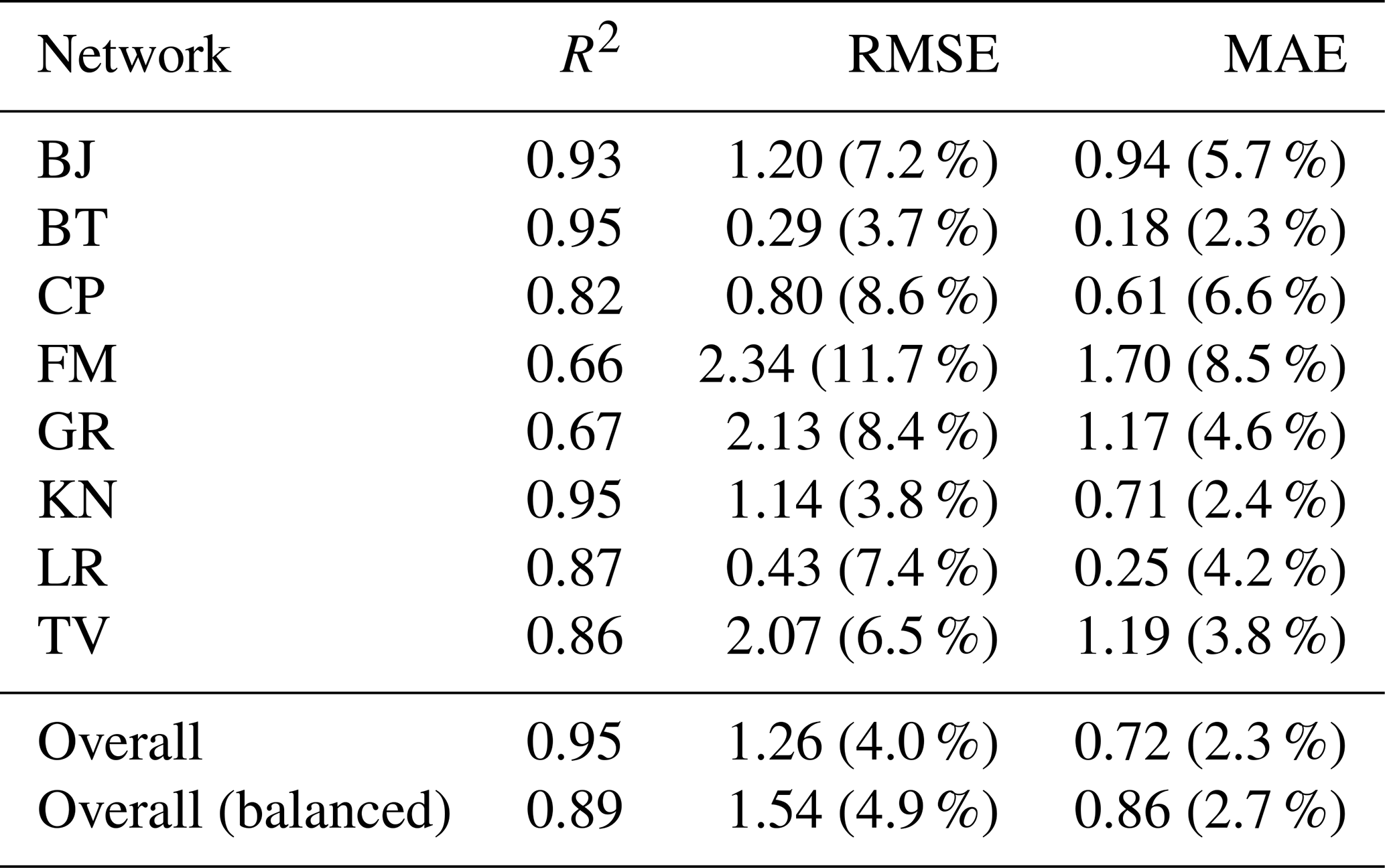
Figure 4 presents the cumulative distribution functions (CDFs) of residuals, highlighting key patterns in SFCC curve-fitting performance across networks and illustrating the residual distributions as a function of soil temperature. Across all networks, residuals are smallest at temperatures below T_f, demonstrating the strong ability of the SFCC fitting to reproduce ε_eff under stable frozen conditions. Residuals increase near T_f, where sparse data in the transitional zone limits the robustness of the curve fitting. Above T_f, residuals remain higher than subfreezing conditions, likely reflecting fluctuations in water content caused by rainfall, transpiration, or drainage. The CDFs exhibit steep slopes near zero across all networks, indicating minimal systematic bias and confirming that most residuals are small, supporting the overall robustness of fitting process. However, underprediction and overprediction are evident in the tails of distributions, corresponding to rapid freezing cycles that the SFCC cannot fully capture.

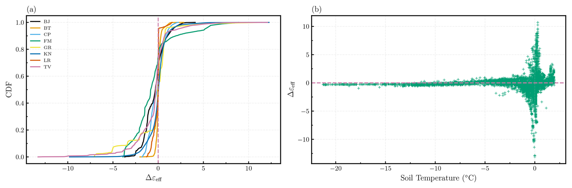
Figure 4 CDFs of residuals across networks (a), showing most residuals are small with steep slopes near zero, indicating minimal bias. Residuals as a function of soil temperature (b), with random subsampling of an equal number of samples per network for balanced representation.

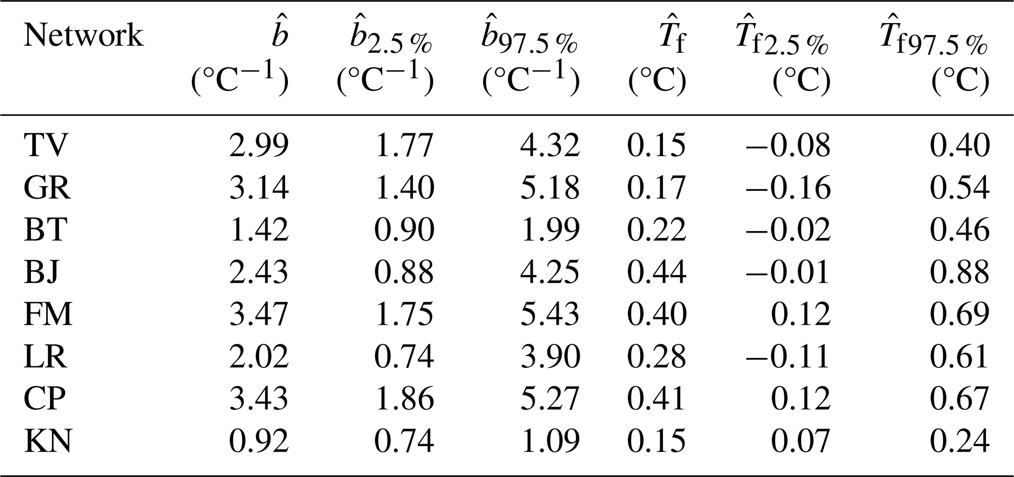
Figure 5 shows the forest plots of T_f (panel a) and b (panel b) across monitoring networks (Detailed network-level soil properties and mean initial water contents are provided in Tables S1 and S2). Black circles denote cycle-level estimates with 95 % confidence intervals, while red squares represent network-level means. Networks are ordered by mean T_f, with sample sizes (N) indicated. To integrate information across sites, networks, and ecozones and stabilize estimates in data-sparse regions, we applied Bayesian hierarchical (partial-pooling) models for both parameters. Table 3 reports posterior means and 95 % credible intervals for b and T_f under hierarchical partial pooling. Across all N=96 freezing cycles, b values ranged from 0.14–5.25, with most cycle-level estimates falling between 0.6 and 2.1 °C⁻¹. Network-level posterior means from the hierarchical model ranged from 0.92–3.47 °C⁻¹, revealing distinct differences in transition sharpness across networks. KN (prairie) and BT (western boreal) exhibited the lowest $\widehat{b}$ (<1.5), indicating gradual soil freezing transitions, while all other networks (BJ, CP, FM, LR, GR, TV) showed higher $\widehat{b}$ (>3), consistent with sharper phase-change behavior. Posterior credible intervals widened with increasing $\widehat{b}$, reflecting higher uncertainty in steep, rapidly changing transitions (Fig. 5). Cycle-level T_f ranged from $-\mathrm{0.54}-\mathrm{0.85}\mathrm{°}\mathrm{C}$, with most estimates between −0.01 and 0.40 °C. Network-level posterior means were slightly positive (0.15−0.44 °C). BJ, FM, LR, and CP exhibited the highest freezing points ($\widehat{T_{\mathrm{f}}}\approx \mathrm{0.40}\mathrm{°}\mathrm{C}$), whereas KN, GR, and TV showed the lowest ($\widehat{T_{\mathrm{f}}}\approx \mathrm{0.15}\mathrm{°}\mathrm{C}$).

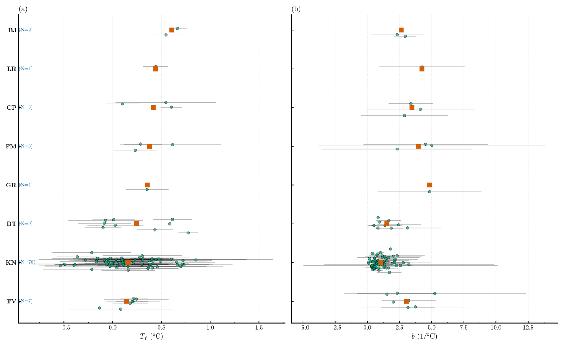
Figure 5 Forest plots showing the distribution of model parameters across networks: freezing point T_f (a) and shape factor b (b). Squares indicate network means, and circles represent individual freezing cycles with vertical bars showing 95 % confidence intervals.

Table 3 Posterior means and 95 % credible intervals of b and T_f from hierarchical partial pooling across networks.

3.2 Model Application to Field Data

To illustrate the application of our SFCC model (Eq. 4) and its integration with in situ data, we present four example sites from different networks and ecozones, each representing a distinct freezing regime: EC17 from KN (prairie; Fig. 6), BT17 from BT (western boreal forest; Fig. 7), BJ01 from BJ (eastern boreal forest; Fig. 8), and GR01 from GR (tundra; Fig. 9). Each example includes two panels: panel (a) shows the fitted SFCC overlaid on in situ soil temperature and ε_eff measurements with T_f marked; panel (b) presents the corresponding time series of soil temperature, freezing probability, ERA5 air temperature, and IMS snow cover. To summarize all networks, Fig. 10 displays the monthly mean freezing probability, with monthly mean air and soil temperatures overlaid on each tile. To compare networks quantitatively, soil states were classified at hourly resolution as frozen if P_frozen>0.75, unfrozen if $P_{\text{frozen}}<{\mathrm{10}}^{-\mathrm{6}}$, and transitional (partially frozen) otherwise. Daily states were assigned by majority rule.

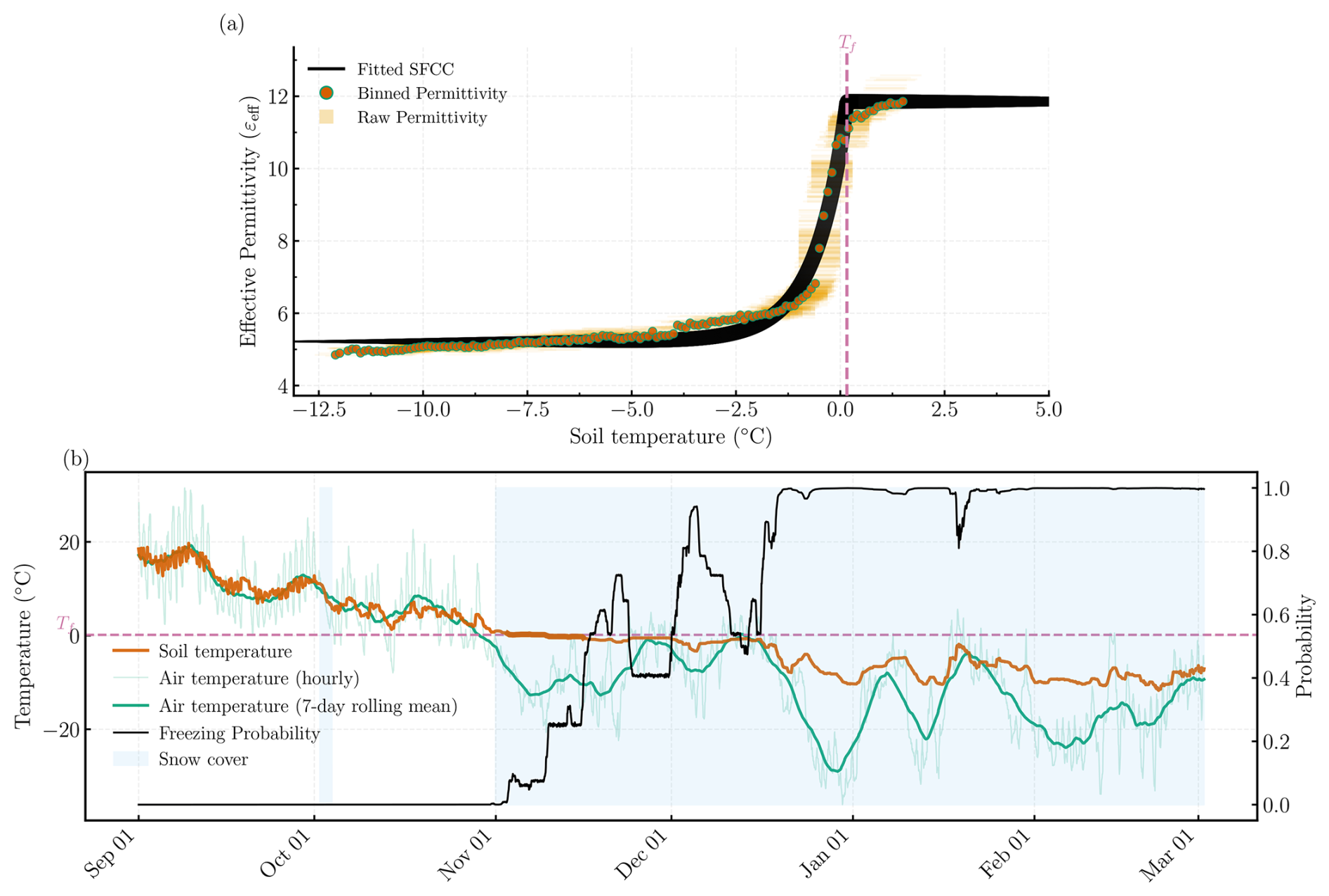
Figure 6 Fitted SFCC (a) and corresponding time series of soil temperature, air temperature, snow cover, and freezing probability (b) for the EC17 site in the Kenaston network (prairie). The site location is available via the interactive map on GitHub: Soil-Temperature-Permittivity-Monitoring-Sites.

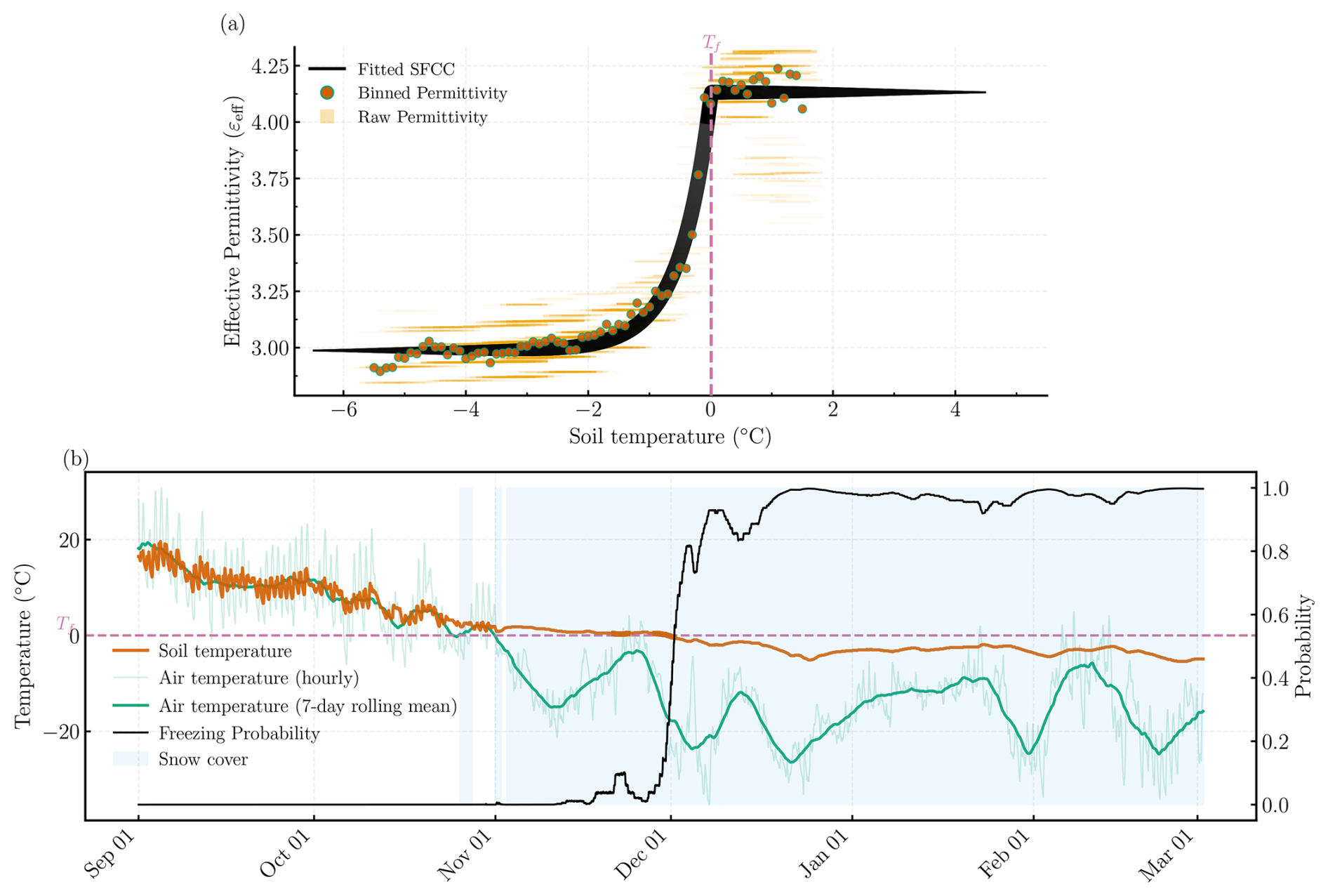
Figure 7 Similar to Fig. 6, but for the BT17 site in the Candle Lake network (western boreal forest).

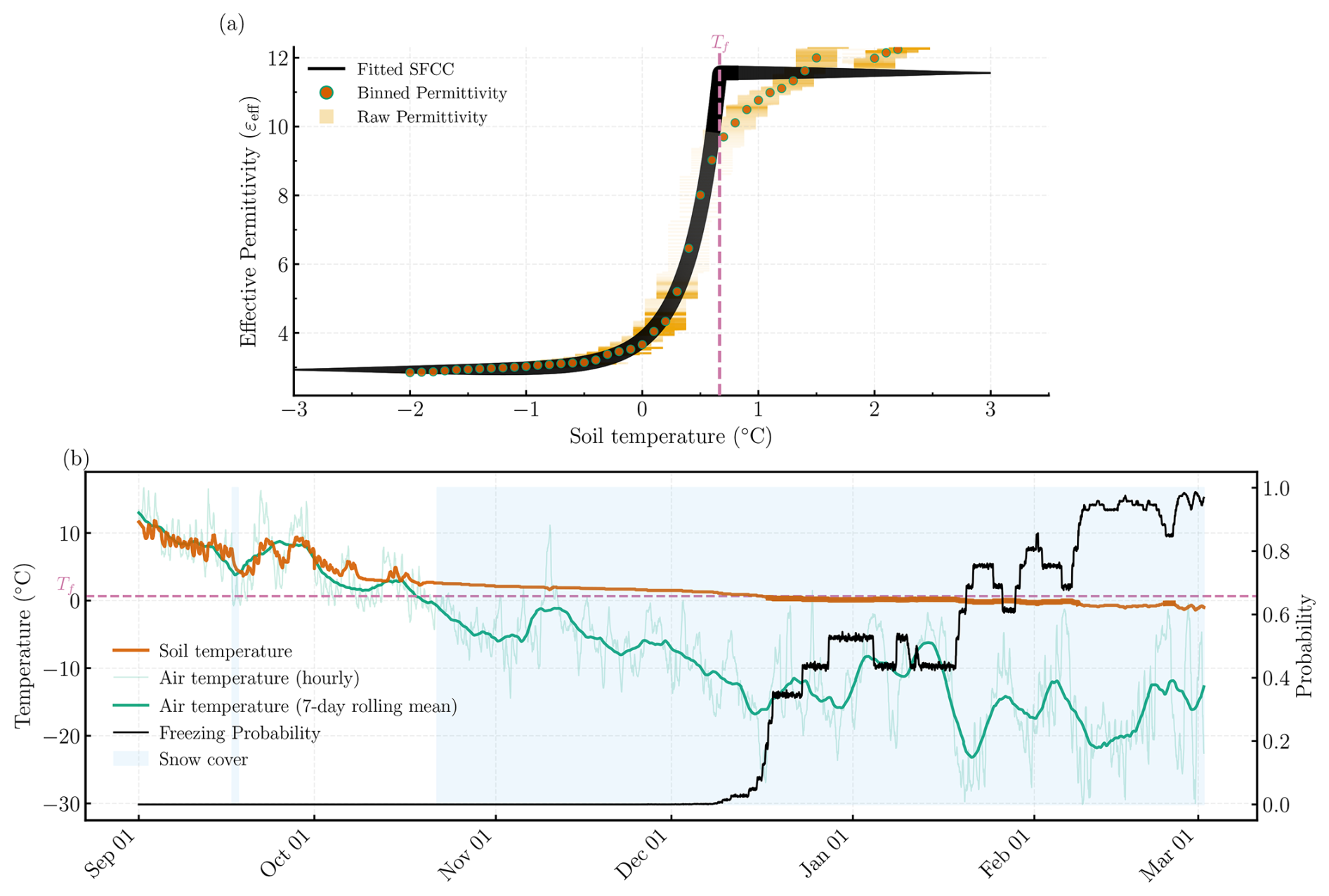
Figure 8 Similar to Fig. 6, but for the BJ01 site in the Baie–James network (eastern boreal forest).

Figure 9 Similar to Fig. 6, but for the GR01 site in the George River network (tundra).

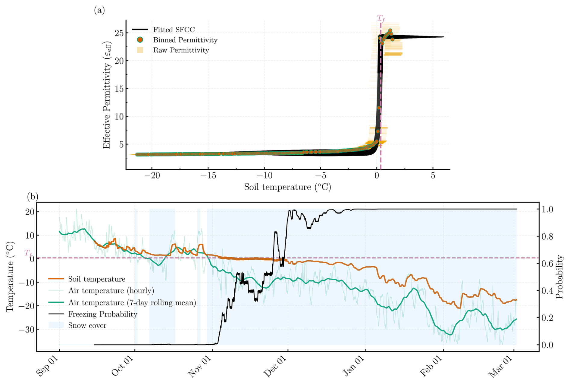
BJ, CP, FM, and LR – located in the eastern boreal forest – remained predominantly unfrozen or partially frozen throughout the freezing season, with no periods of complete freezing despite persistent snow cover (>90 % from December–February) and subzero air temperatures. Their soils stayed near 0 °C, yielding moderate freezing probabilities (P_frozen≤0.65). For instance, FM and CP remained partially frozen for approximately 125 d, while BJ and LR showed shorter transitional periods (≈100 d) with ≈75 unfrozen days. In contrast, BT (western boreal) exhibited extensive freezing from December onward (90 frozen and 30 transitional days), coinciding with subzero air temperatures and complete snow cover. Tundra networks (TV, GR) recorded the coldest soil and air temperatures from December to February (soil and air consistently below −2 and −10 °C, respectively) and persistent snow cover (≈100 %), resulting in almost continuous frozen conditions (P_frozen>0.95) lasting 135 and 95 days for TV and GR respectively. The KN (prairie) network showed an intermediate response: although mean air temperatures ($\approx -\mathrm{3}\mathrm{°}\mathrm{C}$) were comparable to eastern forest networks, soil cooling began earlier (November, T_soil≈0.9 °C) and remained frozen through February (P_frozen>0.9) under shallow or intermittent snow (50 %–95 %). On average, about 70 days were classified as frozen and 60 days as transitional at KN. Overall, while all networks experienced similar subzero air temperatures and persistent snow cover from December to February, only tundra (TV, GR), western boreal (BT), and prairie (KN) networks exhibited sustained frozen states, whereas eastern forest networks (BJ, CP, LR, FM) remained largely in transitional or unfrozen conditions.

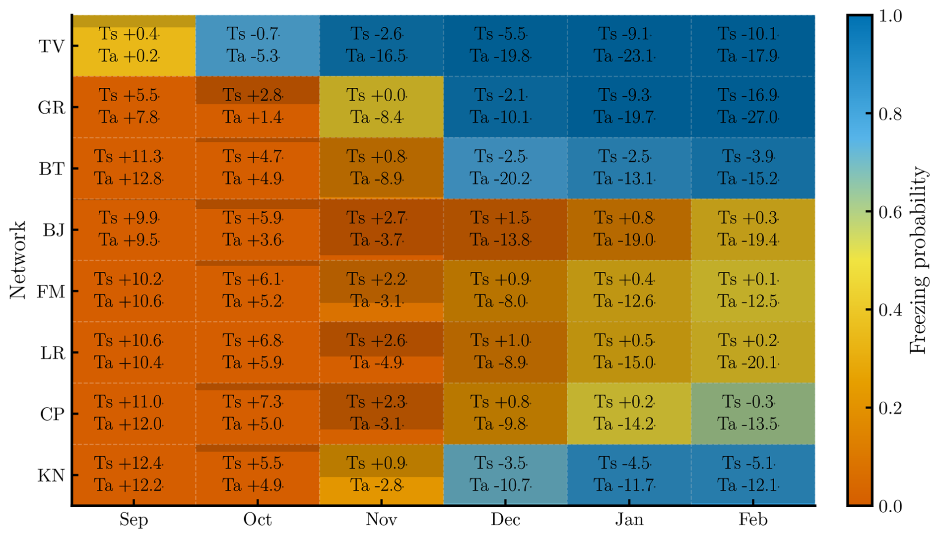
Figure 10 Monthly mean freezing probability for each network. Numbers within cells indicate monthly mean soil and air temperatures (T_s, T_a; °C), while the semi-transparent black fill of each cell represents the monthly mean snow cover (%).

4 Discussion

Our results were generally consistent with the physical factors known to govern the SFCC, particularly soil texture and initial water content (Chai et al., 2018; Bi et al., 2023a). For instance, the KN network, which features the highest clay content (≈27 %), exhibited the most gradual freezing transition (b≈0.92), a result consistent with soil physics principles where small pores and clay surfaces create a broad distribution of matric suctions that allow liquid water to persist at temperatures well below 0 °C (Tian et al., 2014; Zhang et al., 2019; Bi et al., 2023b). Conversely, the GR network, characterized by high initial water content (VWC≈0.40) and sandy texture (>60 % sand, <8 % clay), exhibited a much sharper transition (b≈3.24) (Tian et al., 2014; Zhang et al., 2019; Bi et al., 2023b). It is worth noting that while higher moisture content increases latent heat and delays the onset of freezing – a thermal timing effect clearly visible in our heatmaps where GR begins freezing a month later than the drier TV network – the SFCC b value itself is not a measure of thermal velocity; instead, it reflects the fact that once freezing begins in such coarse, wet soils, the water in large pores transitions to ice abruptly. Similarly, the BT network (b≈1.53) demonstrates that even in sandy soils (>80 % sand), extremely low initial water content (<8 %) can lead to a more gradual transition as the remaining water is held as thin films under higher suction. Despite recognizing these controlling factors, fully disentangling their individual contributions within a natural, open-system environment is inherently challenging. Multiple drivers operate simultaneously and interact nonlinearly, making it difficult to isolate each parameter's effect.

Differences in soil freezing across the networks primarily reflect the combined effects of insulation and soil texture and moisture rather than air temperature alone. Eastern boreal networks (BJ, FM, LR, and CP) remained largely unfrozen throughout winter due to thicker moss and organic layers, denser canopy cover, and higher soil moisture. These features collectively buffer ground heat loss, dampen temperature fluctuations, prolong the zero curtain phase, and keep the soil in a transitional state for extended periods. This interpretation aligns with modeling results from boreal forests in eastern Canada, where soils were shown to remain near 0 °C throughout winter despite mean air temperatures around −16 °C (Oogathoo et al., 2022; Lawrence et al., 2008). Such multilayer insulation reduces conductive and radiative heat exchange between the atmosphere and the soil, thereby limiting frost penetration even under severe cold conditions. In contrast, BT – a dry boreal network with sparse vegetation and thin organic horizons – and KN, which lacks vegetation and organic cover, exhibited earlier and deeper freezing. Tundra networks (GR and TV) experienced prolonged freezing driven by extreme cold and minimal insulation; soil freezing began almost immediately after air temperatures fell below 0 °C, although GR's higher soil moisture delayed freeze onset relative to TV.

A major source of systematic error in permittivity-based sensors is the volume mismatch between the permittivity-sensing domain and the temperature-sensing thermistor (Pardo Lara et al., 2020, 2021). As shown by Pardo Lara et al. (2021), this mismatch can lead to apparent hysteresis and positive freezing-point depression artifacts, where permittivity sensors detect freezing before the thermistor. This occurs because permittivity sensors integrate over a larger, water-biased volume – one that shrinks in wetter soils – while thermistors measure temperature within a much smaller, localized, and water-independent zone (Hansson and Lundin, 2006; Logsdon, 2009; Pardo Lara et al., 2021). Sensor geometry also plays a role. The thermistor in the TEROS12 is embedded in the central needle, minimizing spatial offset, while in the HydraProbe it is located in the base plate. The CS616 lacks a built-in thermistor, requiring external placement, which can exacerbate mismatch effects. However, the primary constraint in estimating T_f remains sensor accuracy. The stated accuracies of ±0.3 °C for the HydraProbe and ±0.5 °C for the TEROS12 are significant within the narrow freezing transitional zone. In our analysis, approximately 90 % of T_f values from the HydraProbe and all values from the TEROS12 and CS616 fell within their respective sensor uncertainty ranges (±2σ °C). This suggests that while volume mismatch may contribute to T_f variability, the observed positive offsets are primarily a function of sensor accuracy bounds rather than a significant systematic bias in the freezing process itself.

One key limitation of this study, as well as any attempt to construct SFCCs from in situ measurements, lies in the assumption that the total water content remains equal to the pre-freezing water content throughout the freezing period (He and Dyck, 2013). In an open system, soil moisture can fluctuate due to rainfall events, intermittent snowmelt, other hydrological inputs, or water redistribution during freezing. This makes identifying a stable “initial” water content (or corresponding ε_eff) particularly challenging. However, we found that averaging the permittivity within a small temperature range (e.g., σ_T °C to 2 °C, where σ_T represents the instrument-specific temperature uncertainty) before the onset of sustained cooling provides a reasonable proxy for the initial moisture conditions. Nevertheless, our results indicate that under freezing conditions – before major thawing or significant water inputs – this assumption holds reasonably well, lending credibility to the use of the derived SFCC parameters to define soil states. Thawing cycles were excluded from this analysis because constructing a reliable STCC from in-situ measurements is not feasible. Once air temperatures rise above 0 °C, the continuous influx of water – primarily from snowmelt – violates the assumption of constant total moisture content required for curve fitting. Because the model cannot identify a stable moisture baseline, the resulting uncertainty in the fitted parameters becomes unacceptably high. Ultimately, this external influx prevents the isolation of temperature-driven phase changes from changes in the total soil water volume. Another practical challenge in applying the SFCC in situ is identifying distinct freezing and thawing periods. In controlled laboratory settings, these phases are straightforward to define due to precisely managed temperature profiles. In natural environments, however, air temperatures fluctuate continuously – often with pronounced diurnal cycles – leading to brief or incomplete freeze–thaw events that are difficult to isolate. These fluctuations are particularly common during the fall and spring shoulder seasons, precisely when soils transition between unfrozen and frozen states. Notably, these transitional periods also provide the critical data needed for deriving T_f and b, making SFCC construction even more challenging. For practical purposes and to improve the reliability of SFCC fitting, we recommend focusing on the main, more sustained freezing periods while disregarding minor, short-lived fluctuations near 0 °C. Although this approach may exclude some small-scale freezing cycles, prioritizing the most clearly defined freeze–thaw phases balances the complexities of natural systems with the need for practical, reliable SFCC parameter estimation. Another challenge encountered during SFCC curve fitting arose when freezing progressed rapidly. The limited temporal resolution of the sensors restricted the number of observations within the transitional zone, reducing the model's ability to resolve steep transitions and increasing the uncertainty in the estimated b values. Consequently, the bootstrap confidence intervals of b widened systematically with increasing b (Fig. 5).

For SFG monitoring, sensors that measure both soil temperature and permittivity are essential. The HydraProbe is advantageous as it directly measures permittivity components, while the TEROS12, despite requiring empirical conversion, offers exceptional energy efficiency. The CS616 is less suitable due to its lack of integrated temperature measurement, undefined permittivity conversion, and poor reliability in cold conditions observed at our CP network. Electrical conductivity (EC) is the most influential factor affecting dielectric sensor accuracy (Seyfried and Murdock, 2004). Increased EC elevates the imaginary permittivity component, leading to signal attenuation and overestimated permittivity values (Seyfried et al., 2005). However, EC values at our sites were generally low – below 0.03 S m⁻¹ in boreal and tundra regions (Fig. S1 in the Supplement) and below 0.2 S m⁻¹ in KN's top 20 cm (Tetlock et al., 2019) – well within acceptable thresholds (0.05–0.14 S m⁻¹ depending on the sensor). Permittivity for TEROS12 and CS616 was derived from raw sensor output using manufacturer-recommended or physically based models. For CS616, we applied the formulation by Kelleners et al. (2005), using generalized calibration coefficients from prior studies (Kelleners et al., 2005; Logsdon, 2009; Hansson and Lundin, 2006). While this may introduce minor biases, the impact on freezing cycle detection is negligible. For TEROS12, we used a third-order polynomial to convert frequency to permittivity (see Eq. A2), though underestimation has been reported in saturated conditions (Cominelli et al., 2024; Fragkos et al., 2024). This is unlikely to affect our analysis, as saturated soils are rare during freezing periods – except at FM, where soil rarely freezes. Importantly, SFCCs can also be constructed directly from raw sensor output, with negligible differences compared to permittivity-based curves (Fig. S2). Both approaches reveal the clear signal drop needed to identify freezing transitions. Soil texture and organic matter may also affect permittivity measurements (Seyfried and Murdock, 2004; Seyfried et al., 2005), but most sites exhibit low clay and organic content, with only a few exceptions in KN and FM. Overall, the permittivity uncertainty is approximately 1–2 units for CS616 and TEROS12, and about 0.1–0.2 units for the HydraProbe – values that are well below the typical permittivity shifts observed during soil freezing and thawing. As long as a discernible permittivity change occurs, the SFCC fitting method can reliably identify the freezing transition. In rare instances where the change is too subtle – e.g., below the measurement uncertainty threshold – the curve-fitting algorithm fails to converge, and such data are automatically excluded from further analysis. Importantly, the SFCC approach is based on the relative change in permittivity with temperature rather than the absolute permittivity values, meaning that minor calibration errors or site-specific variability do not compromise our ability to detect meaningful freezing events. Furthermore, sensor measurement uncertainty (σ_T and σ_ε) was explicitly propagated through Monte Carlo simulations in all probabilistic analyses, ensuring that parameter estimation and freezing probabilities reflect the true uncertainty associated with the sensors.

5 Conclusions

This study applied an SFCC in permittivity–temperature space to enable robust monitoring of seasonally frozen ground (SFG) states using standard dielectric sensors, without the calibration challenges inherent in estimating liquid water content. The key insight from our multi-network analysis is that variations in freezing behavior are dominated by local ground surface properties rather than regional air temperature patterns. Importantly, the transitional (partially frozen) state accounts for the majority of the freezing season in eastern boreal networks and persists for at least one month even in western boreal and tundra networks – dynamics that binary frozen/unfrozen classifications fail to capture. These findings reinforce that air temperature alone cannot predict SFG extent, demonstrating that remote sensing products and land surface models must account for spatial variations in ground surface properties to accurately represent freeze–thaw dynamics at regional scales. The practical value of this approach lies in its compatibility with widely deployed sensor networks and its systematic, straightforward methodology for constructing SFCCs from in situ measurements. Numerous soil monitoring networks across cold regions (e.g., RISMA, SNOTEL, AmeriFlux) already measure both soil temperature and dielectric permittivity. These existing infrastructures could readily adopt the methodology presented in this study to monitor seasonally SFG. This is particularly important given the rapid warming of high-latitude regions and the need for ground-truth evaluation of satellite-based freeze–thaw products, which currently rely primarily on air or soil temperature observations for training and evaluation (Rautiainen et al., 2025; Donahue et al., 2023; Roy et al., 2020; Kou et al., 2017; Gao et al., 2020; Taghipourjavi et al., 2024; Kim et al., 2011; Zhang and Armstrong, 2001).

Appendix A: Sensor Details

A1 CS616 (Campbell Scientific)

The CS616 water content reflectometer measures soil dielectric permittivity by recording the period (in microseconds) of a square-wave oscillation. This oscillation is generated by an electromagnetic pulse that travels along the sensor's 30 cm stainless steel rods, reflects off their ends, and returns to the circuit board to trigger the next pulse. Since the wave velocity depends on the dielectric properties of the surrounding medium, the measured period is directly related to the effective relative permittivity (ε_eff). A physically based equation derived by Kelleners et al. (2005) can be used to convert the raw output to ε_eff:

$$\begin{array}{}\text{(A1)}& {\mathit{\epsilon }}_{\text{eff}}={\left({\displaystyle \frac{(t-\mathrm{2}{t}_{\mathrm{d}})c}{\mathrm{4}L}}\right)}^{\mathrm{2}}\end{array}$$

where $t=\mathit{\tau }/S_{\mathrm{t}}$ is the scaled time period (with S_t=1024 and τ the temperature-corrected raw output in seconds), t_d is the delay time correction (commonly $\mathrm{5.4}\times {\mathrm{10}}^{-\mathrm{9}}\mathrm{s}$), L is the effective rod length (typically 0.261 m for the CS616), and c is the speed of light in a vacuum ($\mathrm{3}\times {\mathrm{10}}^{\mathrm{8}}\mathrm{m}{\mathrm{s}}^{-\mathrm{1}}$) (Hansson and Lundin, 2006; Kelleners et al., 2005; Logsdon, 2009). Although L and t_d can vary slightly between CS616 probes, studies have shown minimal variability (Kelleners et al., 2005; Hansson and Lundin, 2006; Logsdon, 2009). These generalized constants yield acceptable permittivity estimates when sensor-specific calibration is not feasible. Validation against standard reference fluids showed excellent agreement (R²>0.99), and comparisons with TDR, HydraProbe, and Topp's model confirm reliable performance across soils. The accuracy of the CS616 may decline in soils with high EC ($>\mathrm{0.05}\mathrm{S}{\mathrm{m}}^{-\mathrm{1}}$), clay content (>30 %), or organic matter (>5 %) due to signal attenuation and delayed pulse detection. However, the CS616's relatively high operating frequency (∼175 MHz) reduces sensitivity to dispersive effects. The CS616's sensing volume averages permittivity over a non-uniform electric field, which is biased toward wetter zones. While this may slightly inflate permittivity in heterogeneous soils, it helps reduce the influence of small-scale spatial variability. While the CS616 does not measure soil temperature directly, it can be paired with the CS109SS-L sensor for temperature measurements. The CS109SS-L operates over a temperature range of −40 to +70 °C, with an accuracy of ±0.60 °C from −40 to −20 °C and ±0.49 °C from −20 to +70 °C.

A2 TEROS12 (METER Group)

The TEROS12 (METER Group, Inc.) uses capacitance-based technology to estimate soil dielectric permittivity. Operating at 70 MHz, it sends an oscillating signal through three 5.5 cm prongs, which act as a capacitor with the surrounding soil as the dielectric medium. The sensor measures the charge time, which reflects the soil's dielectric properties, and outputs a scaled frequency (RAW) value. This value is converted to ε_eff using a third-order polynomial calibration equation provided in the manual:

$$\begin{array}{}\text{(A2)}& \begin{array}{rl}{\displaystyle }{\mathit{\epsilon }}_{\text{eff}}=& {\displaystyle }(\mathrm{2.887}\times {\mathrm{10}}^{-\mathrm{9}}\times {\text{RAW}}^{\mathrm{3}}-\mathrm{2.080}\times {\mathrm{10}}^{\mathrm{5}}\times {\text{RAW}}^{\mathrm{2}}\\ {\displaystyle }& {\displaystyle }+\mathrm{5.276}\times {\mathrm{10}}^{\mathrm{2}}\times \text{RAW}-\mathrm{43.39}{)}^{\mathrm{2}}\end{array}\end{array}$$

The sensor's reported accuracy is ±1 unit for ${\mathit{\epsilon }}_{\text{eff}}\in [\mathrm{1},\mathrm{40}]$ and ±15 % for values above 40. However, studies have shown that the TEROS 12 can systematically underestimate dielectric permittivity in highly saturated soils and exhibits increased sensitivity under saline conditions (Cominelli et al., 2024; Fragkos et al., 2024). While the manufacturer lists a nominal sensing volume of approximately 1010 cm³, experimental evaluations report a smaller effective volume in moist sand (approximately 423 cm³) and a further reduction in pure water (down to 84 cm³). The sensor also demonstrates strong thermal stability, with temperature-induced changes in permittivity typically remaining below 1 unit across the 10–40 °C range (Cominelli et al., 2024). The TEROS 12 also incorporates an internal thermistor embedded in the central needle to measure temperature. These temperature readings range from $-\mathrm{40}-\mathrm{60}\mathrm{°}\mathrm{C}$, with an accuracy of ±0.5 °C from $-\mathrm{40}-\mathrm{0}\mathrm{°}\mathrm{C}$ and ±0.3 °C from 0–60 °C.

A3 HydraProbe (Stevens Water)

The HydraProbe (Stevens Water Monitoring Systems) uses coaxial impedance dielectric reflectometry to measure the real and imaginary components of complex dielectric permittivity. It features a coaxial waveguide with four stainless steel tines (0.3 cm diameter, 5.7 cm length) arranged in a circle around a central tine, protruding from a 4.2 cm metal base plate. A 50 MHz signal is transmitted through the tines, and the sensor analyzes the amplitude ratio of incident to reflected waves to solve Maxwell's equations. This allows separate estimation of the real (${\mathit{\epsilon }}_{\text{r}}^{\prime }$) and imaginary (${\mathit{\epsilon }}_{\text{r}}^{\prime \prime }$) components of ε_eff, computed as follows (von Hippel, 1955; Topp et al., 1980):

$$\begin{array}{}\text{(A3)}& {\mathit{\epsilon }}_{\text{eff}}={\displaystyle \frac{{\mathit{\epsilon }}_{\text{r}}^{\prime }}{\mathrm{2}}}\left(\mathrm{1}+\sqrt{\mathrm{1}+{\left({\displaystyle \frac{{\mathit{\epsilon }}_{\text{r}}^{\prime \prime }}{{\mathit{\epsilon }}_{\text{r}}^{\prime }}}\right)}^{\mathrm{2}}}\right)\end{array}$$

Laboratory tests confirm that the HydraProbe provides precise and consistent permittivity measurements, with inter-sensor variability typically below ±0.5 units and <1 % coefficient of variation in fluids (Seyfried and Murdock, 2004). It performs reliably up to soil EC values of $\sim \mathrm{0.14}\mathrm{S}{\mathrm{m}}^{-\mathrm{1}}$, beyond which accuracy declines. Loss tangent values above ∼1.45 lead to unstable readings. Despite lacking internal temperature correction, temperature effects are minor – e.g., ∼0.0077 units °C⁻¹ in air and up to $\pm \mathrm{0.06}{\mathrm{m}}^{\mathrm{3}}{\mathrm{m}}^{-\mathrm{3}}$ in saturated clay soils over a 40 °C range. The nominal sensing volume of the HydraProbe is approximately 4.0×10⁴ mm³, but it can expand up to $\sim \mathrm{3.5}\times {\mathrm{10}}^{\mathrm{5}}{\mathrm{mm}}^{\mathrm{3}}$ depending on soil conditions. The effective sensing volume increases in soils with lower permittivity – such as dry or frozen soils – and contracts in wetter soils with higher permittivity. Temperature is measured via a thermistor in contact with the base plate, with a range of −40 °C to +75 °C, an accuracy of ±0.3 °C, and a resolution of 0.1 °C.

Appendix B: Instrumentation Setup

Figure B1 illustrates the insertion depths and orientations of each probe (CS616, HydraProbe, and TEROS12), along with their standard needle lengths. Accompanying the schematic are actual images of the probes to enhance visual recognition and familiarity with their designs.

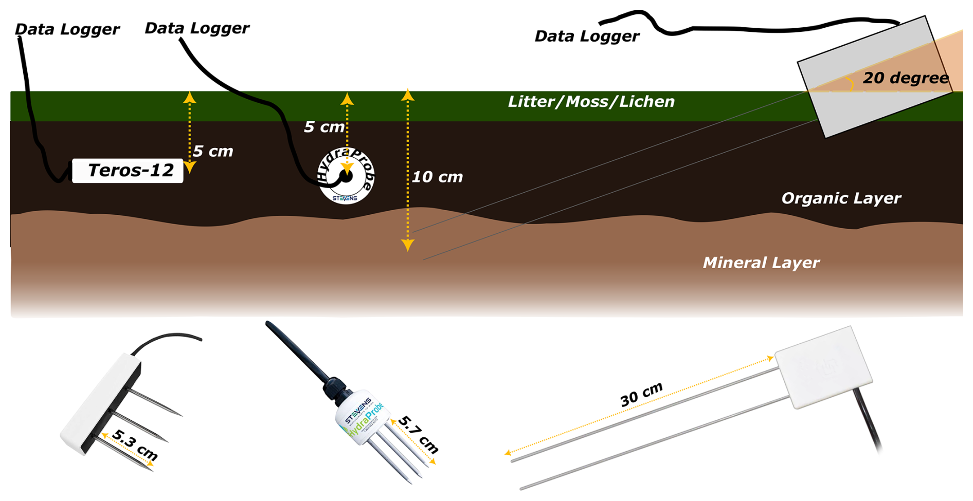
Figure B1 Instrumentation setup for soil moisture probes (CS616, HydraProbe, and TEROS12), with a schematic and corresponding probe images.

Appendix C: Derivation of Bai et al.'s Model in Permittivity–Temperature Space

In this section, we present the detailed steps that transform the Eq. (1) from liquid water content-soil temperature space into permittivity-soil temperature space. The resulting equation expresses the soil's effective permittivity as a function of soil temperature, as shown in Eq.( 4).

C1 For T>T_soil

The simplified form of Eq.( 3) is:

$$\begin{array}{}\text{(C1)}& {\mathit{\theta }}_{\text{lw}}=A{\mathit{\epsilon }}_{\text{eff}}^{\mathit{\alpha }}+B-{\mathit{\theta }}_{\text{ice}}C\end{array}$$

where A, B, and C are defined as:

$$\begin{array}{}\text{(C2)}& {\displaystyle }& {\displaystyle }A={\displaystyle \frac{\mathrm{1}}{{\mathit{\epsilon }}_{\text{lw}}^{\mathit{\alpha }}-{\mathit{\epsilon }}_{\text{air}}^{\mathit{\alpha }}}},\text{(C3)}& {\displaystyle }& {\displaystyle }B={\displaystyle \frac{(n-\mathrm{1}){\mathit{\epsilon }}_{\text{soil}}^{\mathit{\alpha }}-n{\mathit{\epsilon }}_{\text{air}}^{\mathit{\alpha }}}{{\mathit{\epsilon }}_{\text{lw}}^{\mathit{\alpha }}-{\mathit{\epsilon }}_{\text{air}}^{\mathit{\alpha }}}},\text{(C4)}& {\displaystyle }& {\displaystyle }C={\displaystyle \frac{{\mathit{\epsilon }}_{\text{ice}}^{\mathit{\alpha }}-{\mathit{\epsilon }}_{\text{air}}^{\mathit{\alpha }}}{{\mathit{\epsilon }}_{\text{lw}}^{\mathit{\alpha }}-{\mathit{\epsilon }}_{\text{air}}^{\mathit{\alpha }}}}.\end{array}$$

For T>T_soil, we know that θ_ice=0. Therefore, we have:

$$\begin{array}{}\text{(C5)}& {\mathit{\theta }}_{\text{lw}}=A{\mathit{\epsilon }}_{\text{eff}}^{\mathit{\alpha }}+B\end{array}$$

Additionally, the liquid water content θ_int is given by:

$$\begin{array}{}\text{(C6)}& {\mathit{\theta }}_{\text{int}}=A{\mathit{\epsilon }}_{\text{int}}^{\mathit{\alpha }}+B\end{array}$$

Thus, for T>T_soil:

$$\begin{array}{}\text{(C7)}& {\mathit{\epsilon }}_{\text{eff}}={\mathit{\epsilon }}_{\text{int}}\end{array}$$

C2 For T≤T_soil

For T≤T_soil, we can express θ_ice in terms of θ_int and θ_res:

$$\begin{array}{}\text{(C8)}& {\mathit{\theta }}_{\text{ice}}={\mathit{\theta }}_{\text{int}}-{\mathit{\theta }}_{\text{lw}}\end{array}$$

Step 1.

Substitute θ_ice into θ_res:

$$\begin{array}{}\text{(C9)}& {\mathit{\theta }}_{\text{res}}=A{\mathit{\epsilon }}_{\text{res}}^{\mathit{\alpha }}+B-({\mathit{\theta }}_{\text{int}}-{\mathit{\theta }}_{\text{res}})C\end{array}$$

Step 2.

Simplify the equation:

$$\begin{array}{}\text{(C10)}& {\mathit{\theta }}_{\text{res}}=A{\mathit{\epsilon }}_{\text{res}}^{\mathit{\alpha }}+B-{\mathit{\theta }}_{\text{int}}C+{\mathit{\theta }}_{\text{res}}C\end{array}$$

Step 3.

Bring like terms together:

$$\begin{array}{}\text{(C11)}& {\mathit{\theta }}_{\text{res}}(\mathrm{1}-C)=A{\mathit{\epsilon }}_{\text{res}}^{\mathit{\alpha }}+B-{\mathit{\theta }}_{\text{int}}C\end{array}$$

Step 4.

Solve for θ_res:

$$\begin{array}{}\text{(C12)}& {\mathit{\theta }}_{\text{res}}={\displaystyle \frac{A{\mathit{\epsilon }}_{\text{res}}^{\mathit{\alpha }}+B-{\mathit{\theta }}_{\text{int}}C}{\mathrm{1}-C}}\end{array}$$

Step 5.

Similarly, for θ_lw:

$$\begin{array}{}\text{(C13)}& {\mathit{\theta }}_{\text{lw}}={\displaystyle \frac{A{\mathit{\epsilon }}_{\text{eff}}^{\mathit{\alpha }}+B-{\mathit{\theta }}_{\text{int}}C}{\mathrm{1}-C}}\end{array}$$

Step 6.

Substitute these expressions into the Bai et al.'s model for T≤T_soil:

$$\begin{array}{}\text{(C14)}& {\mathit{\theta }}_{\text{lw}}=({\mathit{\theta }}_{\text{int}}-{\mathit{\theta }}_{\text{res}}){\mathrm{e}}^{b(T_{\text{soil}}-T_{\mathrm{f}})}+{\mathit{\theta }}_{\text{res}}\end{array}$$

Step 7.

Express θ_int−θ_res:

$$\begin{array}{}\text{(C15)}& {\mathit{\theta }}_{\text{int}}-{\mathit{\theta }}_{\text{res}}={\displaystyle \frac{A\left({\mathit{\epsilon }}_{\text{int}}^{\mathit{\alpha }}-{\mathit{\epsilon }}_{\text{res}}^{\mathit{\alpha }}\right)}{\mathrm{1}-C}}\end{array}$$

Step 8.

Substitute back and simplify:

$$\begin{array}{}\text{(C16)}& \begin{array}{rl}{\displaystyle \frac{A{\mathit{\epsilon }}_{\text{eff}}^{\mathit{\alpha }}+B-{\mathit{\theta }}_{\text{int}}C}{\mathrm{1}-C}}=& {\displaystyle \frac{A\left({\mathit{\epsilon }}_{\text{int}}^{\mathit{\alpha }}-{\mathit{\epsilon }}_{\text{res}}^{\mathit{\alpha }}\right)}{\mathrm{1}-C}}{\mathrm{e}}^{b(T_{\text{soil}}-T_{\mathrm{f}})}\\ {\displaystyle }& {\displaystyle }+{\displaystyle \frac{A{\mathit{\epsilon }}_{\text{res}}^{\mathit{\alpha }}+B-{\mathit{\theta }}_{\text{int}}C}{\mathrm{1}-C}}\end{array}\end{array}$$

Step 9.

Multiply both sides by 1−C to eliminate denominator:

$$\begin{array}{}\text{(C17)}& \begin{array}{rl}{\displaystyle }A{\mathit{\epsilon }}_{\text{eff}}^{\mathit{\alpha }}+B-{\mathit{\theta }}_{\text{int}}C=& {\displaystyle }A\left({\mathit{\epsilon }}_{\text{int}}^{\mathit{\alpha }}-{\mathit{\epsilon }}_{\text{res}}^{\mathit{\alpha }}\right){\mathrm{e}}^{b(T_{\text{soil}}-T_{\mathrm{f}})}\\ {\displaystyle }& {\displaystyle }+A{\mathit{\epsilon }}_{\text{res}}^{\mathit{\alpha }}+B-{\mathit{\theta }}_{\text{int}}C\end{array}\end{array}$$

Step 10.

Subtract common terms from both sides:

$$\begin{array}{}\text{(C18)}& A{\mathit{\epsilon }}_{\text{eff}}^{\mathit{\alpha }}=A\left({\mathit{\epsilon }}_{\text{int}}^{\mathit{\alpha }}-{\mathit{\epsilon }}_{\text{res}}^{\mathit{\alpha }}\right){\mathrm{e}}^{b(T_{\text{soil}}-T_{\mathrm{f}})}+A{\mathit{\epsilon }}_{\text{res}}^{\mathit{\alpha }}\end{array}$$

Step 11.

Divide both sides by A:

$$\begin{array}{}\text{(C19)}& {\mathit{\epsilon }}_{\text{eff}}^{\mathit{\alpha }}=\left({\mathit{\epsilon }}_{\text{int}}^{\mathit{\alpha }}-{\mathit{\epsilon }}_{\text{res}}^{\mathit{\alpha }}\right){\mathrm{e}}^{b(T_{\text{soil}}-T_{\mathrm{f}})}+{\mathit{\epsilon }}_{\text{res}}^{\mathit{\alpha }}\end{array}$$

Thus, we finally arrive at:

$$\begin{array}{}\text{(C20)}& {\mathit{\epsilon }}_{\text{eff}}={\left(\left({\mathit{\epsilon }}_{\text{int}}^{\mathit{\alpha }}-{\mathit{\epsilon }}_{\text{res}}^{\mathit{\alpha }}\right){\mathrm{e}}^{b(T_{\text{soil}}-T_{\mathrm{f}})}+{\mathit{\epsilon }}_{\text{res}}^{\mathit{\alpha }}\right)}^{\frac{\mathrm{1}}{\mathit{\alpha }}}\end{array}$$