Mapping Antarctic geothermal heat flow with deep neural networks optimized by particle swarm optimization algorithm

Geothermal heat flow (GHF) beneath the Antarctic Ice Sheet (AIS) is a critical basal boundary condition for ice-sheet dynamics modelling and sea-level rise projections. However, it remains insufficiently constrained due to the limited availability of in-situ observations. Here, we propose a deep neural network (DNN) framework that integrates both Particle Swarm Optimization (PSO) and a Bayesian output layer to predict GHF across the entire AIS. Rather than relying on manual or localized parameter selection, the PSO algorithm uses a robust global search mechanism to autonomously optimize key DNN hyperparameters, while the Bayesian layer provides probabilistic GHF predictions and rigorous uncertainty quantification. Model validation based on European GHF datasets demonstrates that the proposed framework consistently outperforms conventional approaches under data-sparse conditions. Then, applying the model to the AIS, we estimate that the Antarctic GHF ranges from 20 to 110 mW m⁻² , with a continental mean value of 65.6 mW m⁻² . Elevated GHF values (generally > 70 mW m⁻² ) dominate much of West Antarctica, while localized high-anomaly zones are identified in parts of East Antarctica, including the Subglacial Lake Vostok region. Uncertainty mapping and the decomposition analysis reveal that most of the uncertainty is inherited from the underlying measurements, indicating that more high-quality observations are needed to further constrain Antarctic GHF predictions.

1 Introduction

Geothermal heat flow (GHF) is the heat energy transferred from Earth's interior to the surface through conduction or convection (Pollack et al., 1993). Beneath the Antarctic Ice Sheet (AIS), it represents a critical heat source that affects the subglacial hydrological system, promotes basal melting, and provides an important boundary condition for numerical models that predict the AIS mass balance and global sea-level change (Obase et al., 2023; Pollard et al., 2005; Seroussi et al., 2017; Wearing et al., 2024; Llubes et al., 2006). Furthermore, the spatial distribution of GHF over Antarctica is crucial for comprehending the past and present tectonic evolution of the continent (Reading et al., 2022).

Due to the severe logistical constraints of operating in the Antarctic interior, direct in-situ borehole GHF measurements remain sparse and unevenly distributed (Fisher et al., 2015; Talalay et al., 2020). Existing estimation approaches generally fall into two categories: on the one hand are those which use a single type of observation to infer GHF, most commonly seismic tomography (Shapiro and Ritzwoller, 2004; An et al., 2015a; Lucazeau, 2019; Shen et al., 2020; Haeger et al., 2022; Hazzard and Richard, 2024) or magnetic anomalies (Fox Maule et al., 2005; Purucker et al., 2012; Martos et al., 2017), although broad tectonic reconstructions have been used as well (Pollard et al., 2005). On the other hand, there are a newer set of statistical methods which integrate multiple types of observational constraints to infer GHF using multivariate similarity analysis (Stål et al., 2021), Bayesian inversion (Lösing et al., 2020) or machine learning (Lösing and Ebbing, 2021). While these approaches exhibit consistency at the continental scale, characterized by higher GHF beneath West Antarctica and lower values in East Antarctica, substantial discrepancies persist at regional scales. The former category is typically constrained by limited data resolution and spatial coverage, as well as by underlying assumptions that may lack universal validity. For instance, seismic tomography-based approaches provide regional-average GHF estimates derived from data with limited sensitivity to upper crustal composition and a coarse lateral resolution of 600–1000 km across Antarctica (Shapiro and Ritzwoller, 2004). In contrast, studies have demonstrated that integrating multiple observables can improve robustness relative to single-dataset approaches (Goutorbe et al., 2011; Lucazeau, 2019). Specifically, Stål et al. (2021) showed that using 14–19 sets of observables produces a misfit of less than 10 mW m⁻² , whereas additional datasets may introduce excessive noise without significantly improving estimates. Consequently, multi-observable approaches require a careful selection of features with adequate Antarctic coverage and strict control over the number of inputs. Moreover, uncertainties in the input data can propagate through the modelling process, and the resulting errors in subglacial GHF substantially impact ice sheet mass balance simulations. Given that the AIS dynamics remain a major source of uncertainty in future sea-level rise projections, ranging from −7.8 to 30.0 cm by 2100 under the RCP8.5 scenario in multi-model ensembles (Seroussi et al., 2020), and potentially exceeding 1 m when marine ice-cliff instability is considered (DeConto and Pollard, 2016), reducing GHF uncertainty is essential for improving the reliability of sea-level predictions.

Recently, deep neural networks (DNNs) have emerged as powerful tools for synthesizing high-dimensional geoscience data because of their formidable ability to capture complex nonlinear relationships. The effectiveness of DNNs has been proven in improving estimates of AIS surface melt (Hu et al., 2021), retrieving sea ice thickness (Herbert et al., 2021), and emulating basal melt rates beneath ice shelves (Burgard et al., 2023). However, current neural network models encounter two primary challenges. First, the performance of DNNs is highly sensitive to numerous hyperparameters; and manual or suboptimal tuning often leads to poor generalization or overfitting. Second, as inherently opaque “black-box” models with limited interpretability, DNNs rarely provide reliable probabilistic estimates or confidence intervals. This lack of formal uncertainty quantification limits their applicability in earth system modelling where the propagation of errors can significantly influence predictive outcomes.

To address these issues, we propose a hybrid DNNs framework that couples PSO to refine parameter selection and incorporates a Bayesian module for robust uncertainty quantification. This integrated approach introduces two key processes aimed at enhancing model generalization and reliability. First, the global search capability of PSO is used to optimize the DNNs hyperparameters, thereby minimizing the objective function and improving predictive accuracy under sparse observational constraints. Second, the Bayesian module enables the decomposition of uncertainty into aleatoric components (originating from input data noise) and epistemic components (inherent in the model architecture and parameters). In the following sections, we detail the dataset construction and modelling methodology, provide an analysis of discrepancies between the new GHF estimates and prior productions, and discuss potential uncertainties along with their implications for future investigations.

2 Data

2.1 Global Heat Flow Dataset

The target variable for this study, GHF, was derived by merging the 2024 release of the International Heat Flow Commission (IHFC) database with the 2019 release of the New Global Heat Flow (NGHF) database (Lucazeau, 2019). This integrated dataset compiles approximately 86 210 in-situ measurements, primarily acquired from bedrock drill holes and thermal probes, with each entry accompanied by a quality assessment grade. We excluded duplicate records between the two databases, entries with missing coordinates or GHF values, and measurements classified as marine, retaining only those with detailed quality assessments (see Supplementary Material S2).

The raw GHF values in the database exhibit an extremely wide range (from −6120 to 100 000 mW m⁻²). However, such extreme values are typically regarded as local anomalies related to non-conductive heat transfer processes or measurement artifacts, and thus lack regional representativeness for continental-scale GHF modelling. Given that continental GHF values rarely exceed 200 mW m⁻², particularly in Antarctica, we implemented a custom interquartile range (IQR) method for outlier detection. By defining the lower and upper bounds using coefficients of 1.15 and 1.25 times the IQR, respectively, we constrained the dataset to a physically plausible range of 0–200 mW m⁻² .

The filtered dataset exhibits significant spatial clustering (Fig. 1). Data coverage is substantially denser in North America, Europe, and parts of East Asia, corresponding to regions with longer histories of geothermal exploration. In contrast, Africa, South America, the Middle East, and Antarctica have markedly sparser coverage, with large areas containing few or no measurements. This geographic bias poses a challenge for empirical GHF modelling, as the training data are not an unbiased representation of Earth's geological diversity, and certain tectonic settings are overrepresented relative to others (Stål et al., 2022). Subsequently, these filtered high-quality point measurements were aggregated onto a 0.5° × 0.5° latitude-longitude grid. Given the variability in data reliability, we assigned quality scores to the GHF data based on original database assessments and computed representative grid values using quality-weighted averages (see Supplement S2), thereby giving greater influence to more reliable measurements within each grid cell. This procedure consolidates the discrete data points into approximately 10 000 representative grid cells. The final processed dataset has a mean GHF of 63.7 mW m⁻² with a standard deviation of 25.3 mW m⁻² (Fig. 1).

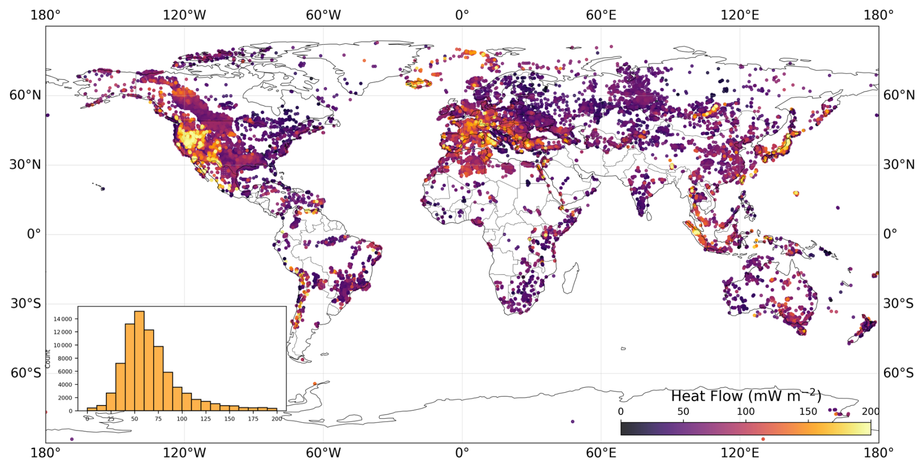
Figure 1 Spatial distribution of global GHF measurements used for model training. The dataset was compiled from the International Heat Flow Commission database and the New Global Heat Flow database (Lucazeau, 2019), filtered using an interquartile range approach to constrain values within 0–200 mW m⁻².

2.2 Geophysical Features

The spatial distribution of GHF is governed by a complex interaction between the geological and geophysical properties of the lithosphere (Goutorbe et al., 2011; Lucazeau, 2019). Table 1 summarizes the geophysical and geological features utilized for model prediction, along with their respective data sources. Also, we provide maps of all input features in both global and Antarctic polar stereographic projections in the Supplement S1.

Table 1 Geophysical features and data sources employed in this study.

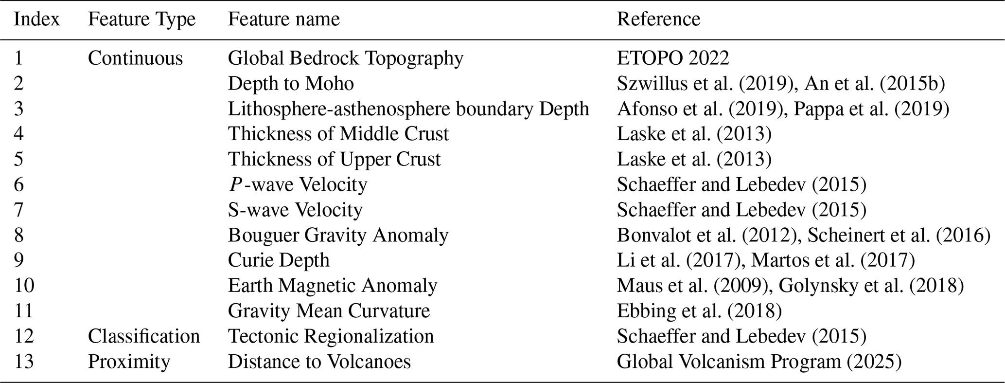
Note: Where two references are listed, the first provides global coverage and the second supplements with Antarctic-specific data offering higher regional resolution.

To facilitate direct comparison with previous studies, we incorporated several legacy datasets that have served as standard inputs in Antarctic GHF modelling. Primary controls on GHF include Moho depth, lithosphere-asthenosphere boundary (LAB) depth, and crustal thickness. Crustal thickness largely determines the magnitude of radiogenic heat production from radioactive isotopes (U, Th, and K), which represents a primary component of GHF. We utilized crustal thickness data from the CRUST1.0 model (Laske et al., 2013), which provides detailed layered crustal structure on a global 1° × 1° grid. In regions where seismic constraints remain sparse, such as Antarctica, CRUST1.0 leverages gravity-constrained interpolation methods with demonstrated reliability. Moho depth was derived from Szwillus et al. (2019), whose geostatistical kriging approach provides a transparent interpolation methodology with explicit uncertainty bounds. For the Antarctic regions, we augmented these data with the AN-Crust model (An et al., 2015b), which is constructed from surface wave tomography and constrained by regional receiver function data and achieves a higher resolution in Antarctica compared to global models. The LAB depth defines the thermal boundary layer of the lithosphere, where a shallower LAB typically correlates with a higher geothermal gradient. LAB depth data were obtained from the LithoRef18 global model (Afonso et al., 2019), with Antarctic regions supplemented by the AN-LAB model from An et al. (2015a). Both models are based on joint inversion of seismic and gravity data, effectively characterizing the spatial distribution of the lithospheric thermal boundary layer. Seismic wave velocities serve as effective proxies for the thermal state of the crust and upper mantle due to their inverse correlation with temperature. We selected shear-wave velocity (V_s) and compressional-wave velocity (V_p) data at 150 km depth from the Schaeffer and Lebedev (2015) model, which is constructed from cluster analysis of global surface wave tomography without requiring a priori assumptions about Earth's structure, thus objectively reflecting upper mantle velocity anomalies beneath Antarctica. The curie depth, representing the isotherm of approximately 580 °C, provides a direct constraint on the geothermal gradient. Then,we adopted the GCDM model (Li et al., 2017), which is inverted from EMAG2 magnetic anomaly data. To address the limited coverage of GCDM in the Antarctic interior, we supplemented it with the Curie depth model from Martos et al. (2017), which provides explicit uncertainty bounds. Potential field datasets incorporated three categories: The Bouguer gravity anomaly input was derived from the global World Gravity Map 2012 (Bonvalot et al., 2012), with data for the Antarctic region substituted by the high-resolution, ice-sheet-adapted gravity model of Scheinert et al. (2016). Magnetic anomaly utilized the EMAG2v3 global compilation (Maus et al., 2009) combined with the Antarctic ADMAP2 model (Golynsky et al., 2018). Gravity mean curvature was derived from GOCE satellite gravity gradient data following the methodology of Ebbing et al. (2018). Topographic data were sourced from the ETOPO2022 model (NOAA, 2022), which integrates multi-source data including airborne LiDAR, satellite remote sensing, and shipborne bathymetry. This model provides significantly improved topographic resolution in Antarctic regions, enabling accurate delineation of subglacial topographic features. To incorporate tectonic context, we incorporated the six-domain tectonic province classification from Schaeffer and Lebedev (2015), derived from cluster analysis of global surface wave tomography. Volcanic activity serves as an important indicator of elevated advective heat transport. To account for advective heat transport, distances to Holocene volcanoes were converted into thermal influence indices using an exponential decay function. The global volcano location data are derived from the Global Volcanism Program (2013).

All predictor variables were standardized to a uniform 0.5° × 0.5° grid via ordinary kriging. The final feature set comprises continuous variables, categorical variables, and thermal proximity indices.

3 Methods

The comprehensive methodological workflow for modelling GHF across Antarctica is depicted in Fig. 2. The proposed framework is organized into four primary stages: (1) data collection, compiling global GHF measurements and geophysical input features; (2) preprocessing, including quality filtering, outlier removal, and gridding to 0.5° × 0.5° resolution; (3) model construction, utilizing a DNN architecture optimized via PSO and integrated with Bayesian uncertainty quantification; and (4) prediction and uncertainty mapping across the Antarctic continent.

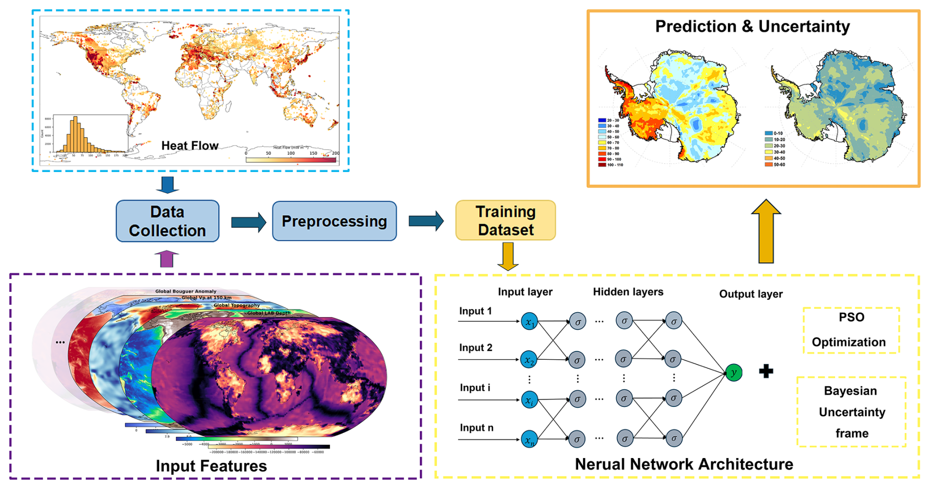
Figure 2 Schematic workflow of the PSO-Bayesian deep neural network framework for Antarctic GHF prediction. The upper-left panel shows global GHF measurements used for training. The lower-left panel displays examples of geophysical input features. The central component illustrates the neural network architecture, consisting of an input layer receiving multiple geophysical variables, hidden layers with optimized depth and width, and an output layer producing GHF predictions. The network hyperparameters are optimized using particle swarm optimization (PSO), while a Bayesian framework enables uncertainty quantification. The upper-right panel presents the final outputs: predicted GHF distribution and associated uncertainty estimates across Antarctica.

3.1 Deep Neural Networks

Neural networks are increasingly utilized in the Earth sciences for their efficacy to effectively model complex, non-linear relationships and automatically extract hierarchical features from multidimensional datasets (Hastie et al., 2009). In this study, we adopt a DNN based on the classic multilayer perception. The DNN architecture comprises an input layer, multiple hidden layers, and an output layer. All hidden layers use the Rectified Linear Unit (ReLU) activation function to mitigate the vanishing gradient problem and enhance computational efficiency. Compared to shallower architectures, increasing the depth with more hidden layers allows the model to learn progressively more abstract and intricate patterns from the input features.

A key advantage of DNNs and other supervised machine learning techniques is their ability to reproduce complex non-linear systems without requiring predefined governing equations. Instead, performance relies on a supervised training phase where the weights and biases of neurons are iteratively adjusted. During training, the model iteratively tunes these parameters using the backpropagation algorithm, guided by the Adam optimizer (Kingma and Ba, 2015), to minimize a mean-squared-error loss function between the predicted and observed GHF values. The training dataset is randomly partitioned into mini-batches, and the weights are optimized batch by batch. A complete cycle through all mini batches defines one training epoch, with the weights and biases being continuously refined over multiple epochs. Concurrently, the model's performance on a separate validation dataset is monitored to track its ability to generalize to unseen data. Upon completion of training, the model's final performance is assessed using a test dataset that was entirely withheld from the training and validation processes.

3.2 Bayesian Uncertainty Quantification Framework

Traditional neural networks optimize a deterministic set of weights via gradient-based algorithms. Consequently, they provide only point estimates for a given input, lacking the inherent capacity to quantify the reliability or confidence intervals of their predictions. To address this limitation, we integrate a Bayesian deep learning framework that enables principled uncertainty quantification by decomposing predictive uncertainty into its aleatoric and epistemic components (Kendall and Gal, 2017; Gal and Ghahramani, 2016).

Unlike standard DNNs, Bayesian Neural Networks treat weights as probability distributions rather than fixed values. We implement a computationally efficient hybrid architecture where hidden layers utilize deterministic weights, while the output layer employs Bayesian linear transformations with Gaussian priors. The posterior distributions are approximated via variational inference (VI) using the reparameterization trick (Blundell et al., 2015).

Total predictive uncertainty is decomposed into two distinct components. Aleatoric uncertainty represents irreducible noise inherent in the observations, arising from measurement errors and unresolved physical processes. To capture this data-dependent uncertainty, our network is designed to output both the predicted mean and the predicted variance. Conversely, epistemic uncertainty reflects model uncertainty stemming from limited training data, quantified through the variance of predictions obtained via Monte Carlo sampling (T=50 samples) from the approximate posterior distribution. The total predictive uncertainty is computed as the sum of these two components:

$$\begin{array}{}\text{(1)}& {\mathit{\sigma }}_{\mathrm{total}}^{\mathrm{2}}={\mathit{\sigma }}_{\mathrm{aleatoric}}^{\mathrm{2}}+{\mathit{\sigma }}_{\mathrm{epistemic}}^{\mathrm{2}}\end{array}$$

The model is optimized by maximizing the Evidence Lower Bound (ELBO), which combines the negative log-likelihood with the Kullback-Leibler (KL) divergence between the variational posterior and prior distributions. The KL weighting coefficient β and prior variance ${\mathit{\sigma }}_{\mathrm{p}}^{\mathrm{2}}$ are optimized via PSO alongside other hyperparameters. Detailed mathematical derivations, ELBO loss function formulations, KL divergence calculations, and reparameterization techniques are provided in Supplement S3.

3.3 Particle Swarm Optimization

The predictive performance of DNN is highly sensitive to hyperparameter configurations, rendering manual hyperparameter tuning inefficient and suboptimal. To address this challenge, this study employs the Particle Swarm Optimization (PSO) algorithm, a population-based stochastic optimization technique inspired by the collective social behavior of bird flocks (Kennedy and Eberhart, 1995), to systematically search for optimal hyperparameter combinations. In the PSO implementation, each “particle” within the swarm represents a unique candidate set of hyperparameters, encompassing the number of hidden layers, neuron count per layer, initial learning rate, batch size, and regularization strength. The particle swarm iteratively explores the hyperparameter space, with each particle adjusting its trajectory based on its personal best solution and the global best solution to minimize the loss function on the validation set, thereby optimizing both predictive accuracy and generalization capability. The velocity and position updates for particle i follow the equations

$$\begin{array}{}\text{(2)}& {\displaystyle }{v}_i\left(t+\mathrm{1}\right)=\mathit{\omega }{v}_i\left(t\right)+c_{\mathrm{1}}{r}_{\mathrm{1}}\left(p_{\mathrm{i}}-x_i\left(t\right)\right)+c_{\mathrm{2}}{r}_{\mathrm{2}}\left(g-x_i\left(t\right)\right)\text{(3)}& {\displaystyle }{x}_i\left(t+\mathrm{1}\right)=x_i\left(t\right)+v_i\left(t+\mathrm{1}\right)\end{array}$$

where v_i(t) and x_i(t) represent the velocity and position of the ith particle at iteration t, respectively; p_i denotes the individual optimal position, g is the global optimal position. The inertia coefficient ω controls momentum preservation, while cognitive coefficients c₁ and social coefficients c₂ weight the attraction toward p_i and g. r₁ and r₂ are random numbers between [0,1] to provide randomness to enhance the diversity of the search. In this study, PSO was employed to optimize the DNN's hyperparameters within the following ranges: number of hidden layers (3–6), neurons per hidden layer (32–128), learning rate (0.0001–0.01), batch size (32–128), dropout rate (0.05–0.3), KL weight ($\mathrm{1}\times {\mathrm{10}}^{-\mathrm{5}}$–$\mathrm{1}\times {\mathrm{10}}^{-\mathrm{3}}$), prior variance (0.5–1.5), and L2 regularization strength ($\mathrm{1}\times {\mathrm{10}}^{-\mathrm{5}}$–$\mathrm{1}\times {\mathrm{10}}^{-\mathrm{4}}$).

3.4 Training Process

To satisfy neural network input requirements and optimize training performance, we implemented a two-step preprocessing pipeline for the feature set. First, label encoding was applied to categorical variables, converting non-numerical labels into unique integer representations. Second, all continuous predictor variables and the target GHF variable underwent standardization by subtracting the mean and dividing by the standard deviation, with statistical parameters computed exclusively from training data within each cross-validation fold to prevent data leakage. This standardization step is crucial for the gradient-based Adam optimizer, ensuring all features operate on similar numerical scales, thereby stabilizing the training process and mitigating risks of slow convergence or gradient explosion.

To evaluate model performance robustly and minimize bias associated with single train-test splits, we employed a 5-fold cross-validation framework. The dataset was partitioned into five mutually exclusive folds, with the model trained five times, each iteration using one-fold as the test set and the remaining four as the training set. During each training iteration, the Adam optimizer was employed to leverage its computational efficiency and adaptive learning rate characteristics. To control model complexity and mitigate overfitting, we implemented a multi-faceted regularization strategy: (1) L2 regularization (weight decay) was applied to penalize large weight magnitudes and encourage simpler model representations; (2) batch normalization was implemented after each hidden layer to stabilize training dynamics and accelerate convergence; (3) dropout layers were incorporated between hidden layers to randomly deactivate neurons during training, reducing co-adaptation and improving generalization; and (4) an early stopping mechanism was established, terminating training if validation loss failed to decrease for 10 consecutive epochs, with model weights corresponding to the lowest validation loss retained.

In the final inference stage, an ensemble model was constructed using the five independent models generated through cross-validation to provide comprehensive coverage across the entire Antarctic continent. The final GHF prediction at any given location represents the arithmetic mean of the five model outputs, with this ensemble strategy enhancing predictive accuracy and robustness by averaging individual model biases. The uncertainty quantification follows the Bayesian framework described in Sect. 3.2, where aleatoric uncertainty is derived from the predicted variance output of each model, and epistemic uncertainty is quantified through Monte Carlo sampling from the Bayesian posterior. The ensemble-level total uncertainty at each grid point incorporates both the within-model Bayesian uncertainty and the between-model variance, computed as the quadrature sum of these components.

3.5 Model Evaluation Metrics

To assess the predictive performance of the model, we employed two complementary evaluation metrics: the coefficient of determination (R²) and the normalized root mean square error (NRMSE). The combination of these metrics, together with a robust cross-validation procedure to avoid overfitting, provides a widely recognized framework for evaluating goodness-of-fit in regression analysis (Branco et al., 2016).

R² quantifies the proportion of variance in the observed GHF values that is explained by the model predictions. In this study, we adopt the coefficient of determination, defined based on the residual sum of squares, which is the standard metric in regression analysis and machine learning applications:

$$\begin{array}{}\text{(4)}& R^{\mathrm{2}}=\mathrm{1}-{\displaystyle \frac{{\sum }_{i=\mathrm{1}}^n(y_i-{\widehat{y}}_i{)}^{\mathrm{2}}}{{\sum }_{i=\mathrm{1}}^n(y_i-{)}^{\mathrm{2}}}}\end{array}$$

where y_i is the observed value, ${\widehat{y}}_i$ is the predicted value, is the mean of the observed value, and n is the sample size. The value typically ranges from 0 to 1, where 1 indicates perfect prediction, and 0 indicates that the model performs no better than simply predicting the mean. Notably, R² can become negative when the model predictions are worse than the mean baseline, which can occur with poorly specified models or when evaluating on out-of-sample data.

NRMSE is a widely used metric for evaluating the relative magnitude of prediction errors. By normalizing the error relative to the mean of the predicted values, it effectively eliminates the influence of data magnitude. The formula is given as follows:

$$\begin{array}{}\text{(5)}& \mathrm{NRMSE}={\displaystyle \frac{\sqrt{\frac{\mathrm{1}}{n}{\sum }_{i=\mathrm{1}}^n(y_i-{\widehat{y}}_i{)}^{\mathrm{2}}}}{\widehat{y}}}\end{array}$$

where y_i is the observed value, ${\widehat{y}}_i$ is the predicted value, is the mean of the predicted value, and n is the sample size. In this study, the NRMSE reflects the proportion of prediction error relative to the level of GHF prediction. For example, an error of 0.15 can be interpreted as an average relative error of 15 % in the prediction.

4 Results

4.1 Collinearity Analysis

Collinearity analysis of input features is a critical step in constructing multivariate regression models, as it ensures both numerical stability and physical interpretability. High linear correlations among predictor variables, known as multicollinearity, inflate the variance of regression coefficients, thereby compromising predictive performance. Given that GHF is governed by complex interactions among multiple geophysical factors, detecting and mitigating such correlations is essential. To quantify multicollinearity, we employed the Variance Inflation Factor (VIF), which measures the degree to which the variance of regression coefficients increases due to multicollinearity. For the ith predictor variable, VIF is defined as:

$$\begin{array}{}\text{(6)}& {\mathrm{VIF}}_i={\displaystyle \frac{\mathrm{1}}{\mathrm{1}-R_i^{\mathrm{2}}}}\end{array}$$

where $R_i^{\mathrm{2}}$ represents the coefficient of determination obtained from regressing the ith predictor against all other predictor variables. Based on the VIF threshold range of 5–10 recommended by Hair et al. (2010), a threshold of 8.0 was adopted in this study. Variables with VIF values exceeding 8.0 were considered to exhibit problematic multicollinearity and were iteratively removed.

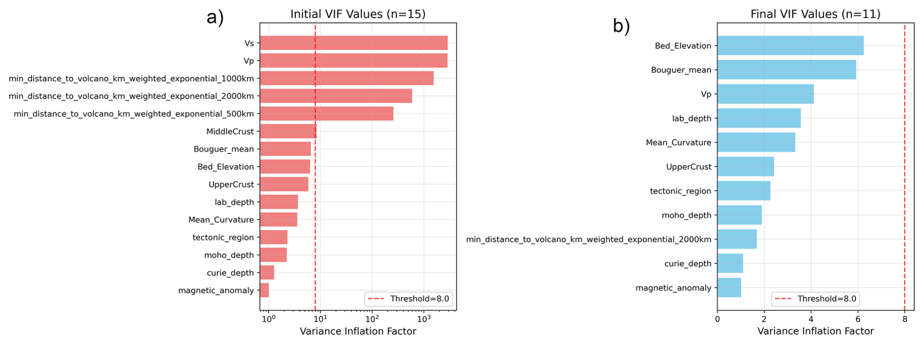
Figure 3 VIF analysis for multicollinearity detection among input features. (a) Initial VIF values for all 15 candidate features. (b) Final VIF values after iterative removal of highly collinear features. Four variables were excluded: V_p, V_s, and two volcano distance-weighting features (500 and 1000 km decay parameters).

Initial assessment of 15 predictor variables revealed severe multicollinearity among several features (Fig. 3a). Most notably, P-wave velocity (V_p) and S-wave velocity (V_s) exhibited extremely high VIF values exceeding 1000, reflecting their strong physical interdependence as both are fundamentally controlled by the same lithospheric properties. Additionally, the distance-weighted volcano proximity features showed substantial collinearity, with the 1000 and 500 km exponential decay variants displaying VIF values above 100, indicating redundant spatial information at different decay scales. Following an iterative removal procedure, four variables exhibiting the highest VIF values were excluded: V_p, V_s, and two volcano distance-weighted features (500 and 1000 km decay parameters). The retained 2000 km decay variant adequately captures the regional thermal influence of volcanic activity while minimizing redundancy.

4.2 PSO Parameter Sensitivity Analysis

PSO is extensively applied in function optimization and neural network training. The selection of PSO parameters is crucial for algorithm performance and efficiency, as these parameters exhibit interdependencies across different parameter spaces. Typically, parameter selection relies on empirical knowledge. This study employed the pyswarm implementation, with adjustable parameters including particle number (m), inertia weight (w), learning factors (c₁ and c₂), and maximum iterations. The inertia weight controls the influence of a particle's previous velocity on its current trajectory, thereby achieving a balance between global and local search capabilities. We adopted the linearly decreasing weight proposed by Shi and Eberhart (1998):

$$\begin{array}{}\text{(7)}& w=w_{\max }-{\displaystyle \frac{w_{\max }-w_{\min }}{T_{\max }}}t\end{array}$$

where w_max and w_min represent the maximum and minimum inertia weights (typically set to 0.9 and 0.4, respectively), t denotes the current iteration number, and T_max represents the maximum iteration count. The learning factors c₁ and c₂ determine the stochastic accelerations toward personal best and global best positions, respectively. Previous studies have proposed various recommendations: Kennedy and Eberhart (1995) suggested setting both to 2, while subsequent researchers argued for asymmetric values, with experimental evidence supporting c₁= 2.8. Suganthan (1999) tested a method for linearly decreasing both acceleration coefficients over time but observed that fixing acceleration coefficients at 2 produced superior solutions. Regarding particle number, He et al. (2016) demonstrated through their experiments that a particle number of 20 is sufficient for standard optimization problems, whereas more complex scenarios may require up to 50 particles.

Based on prior research, this study designed four experimental configurations with different c₁, c₂, and m values to determine optimal parameter settings: Config1 ($c_{\mathrm{1}}=c_{\mathrm{2}}=$ 2, m= 20), Config2 ($c_{\mathrm{1}}=c_{\mathrm{2}}=$ 2, m= 50), Config3 (c₁= 2.8, c₂= 1.0, m= 20), and Config4 (c₁= 2.8, c₂= 1.0, m= 50). The experimental procedure involved PSO-based neural network hyperparameter optimization with the objective of minimizing RMSE on the validation set. Each configuration underwent 100 iterations with linearly decreasing inertia weight while maintaining fixed learning factors and particle numbers. Convergence curves showing RMSE variation with iteration count are presented in Fig. 4.

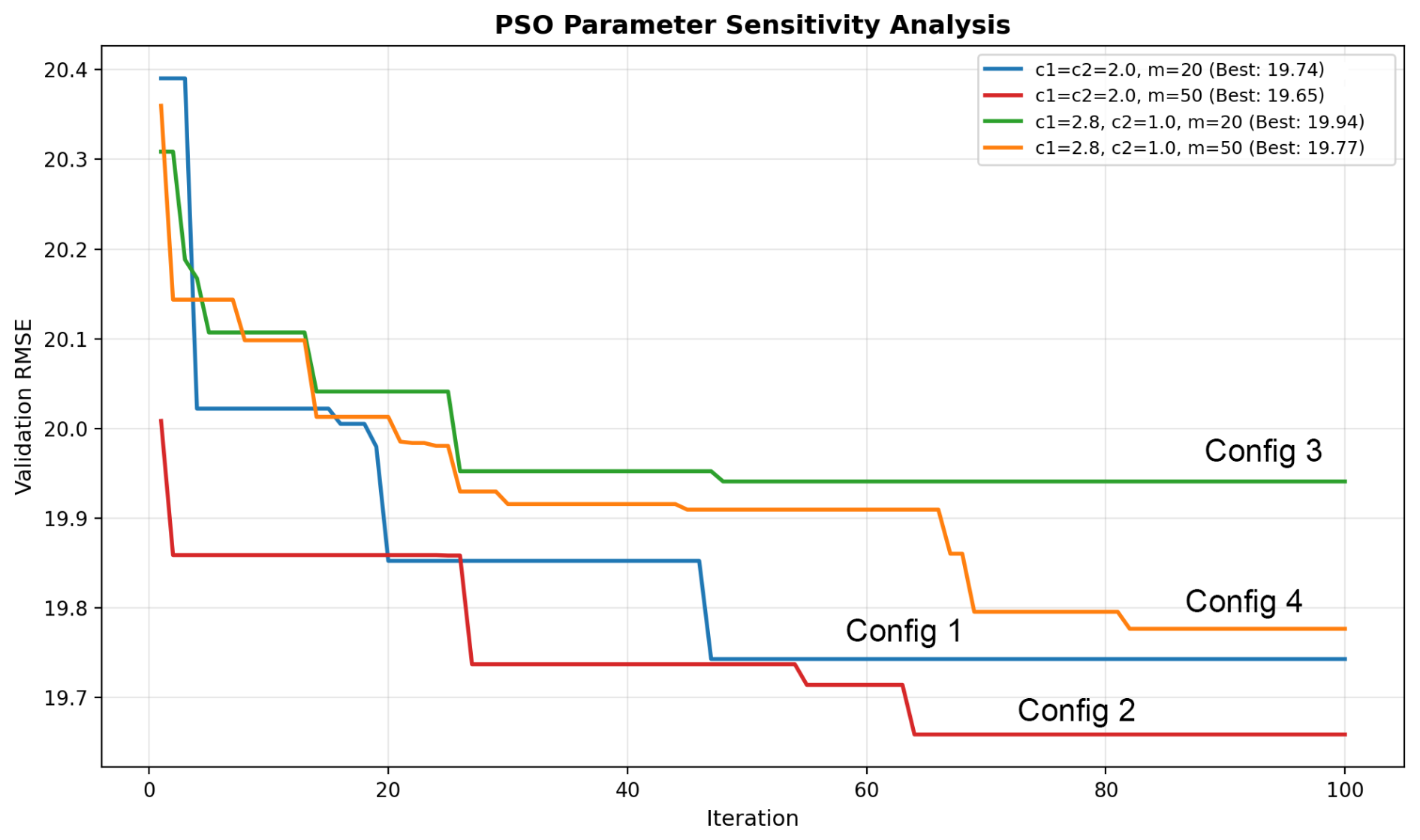
Figure 4 PSO parameter sensitivity analysis showing validation RMSE convergence curves over 100 iterations for four configurations with different acceleration coefficients (c₁, c₂) and particle numbers (m).

Figure 4 illustrates RMSE trends across 100 iterations for the four configurations. Config2 ($c_{\mathrm{1}}=c_{\mathrm{2}}=$ 2.0, m= 20) achieved the lowest final RMSE of 19.65 mW m⁻² , followed by Config1 (19.74 mW m⁻²), Config4 (19.77 mW m⁻²), and Config3 (19.94 mW m⁻²). The symmetric acceleration coefficients setting ($c_{\mathrm{1}}=c_{\mathrm{2}}=$ 2.0) consistently outperformed the asymmetric configuration. Notably, the narrow performance differences (less than 0.3 mW m⁻² between best and worst configurations) suggest that for this specific GHF prediction problem, the optimization landscape is relatively smooth, allowing all configurations to converge to similar solutions. Nevertheless, Config2 was selected as the optimal configuration for subsequent model training based on its lowest validation RMSE.

4.3 GHF Prediction with Limited Local Data

A primary challenge for this framework involves predicting GHF in regions with sparse in-situ measurements, such as Antarctica. To quantitatively assess model performance under such data-constrained conditions and address validation requirements in data-scarce regions, we adopted the training density analysis approach proposed by Rezvanbehbahani et al. (2017). This method systematically evaluates the relationship between prediction accuracy and local training data availability through a training density defined for a specified Region of Interest (ROI):

$$\begin{array}{}\text{(8)}& {\mathit{\rho }}_{\mathrm{ROI}}=\left(\mathrm{1}-{\displaystyle \frac{N_{\mathrm{ROI}}^{\prime }}{N_{\mathrm{ROI}}}}\right)\times \mathrm{100}\mathit{\%}\end{array}$$

where N_ROI represents the total number of data points within the target ROI, and $N_{\mathrm{ROI}}^{\prime }$ denotes the number of data points within the ROI that are deliberately excluded from the training set and reserved exclusively for model validation.

This experiment utilized the high-density European GHF record as the test dataset. To determine the ROI, we implemented a grid search algorithm to identify the circular region (radius = 1300 km) containing the maximum density of data points within the study area (0–45° E, 28–52° N). The optimal circle center was located at approximately 21° E, 43° N, encompassing the data-rich regions of Central and Eastern Europe. Data points were randomly sampled from the ROI at 10 % increments (10 % to 90 %) and combined with all data points outside the ROI to form the training set. Simultaneously, the remaining data points within the ROI served as an independent validation set to evaluate model prediction performance at corresponding densities. To ensure statistical robustness, this random sampling process was repeated five times at each density level, with corresponding calculations of mean values and standard deviations for performance metrics.

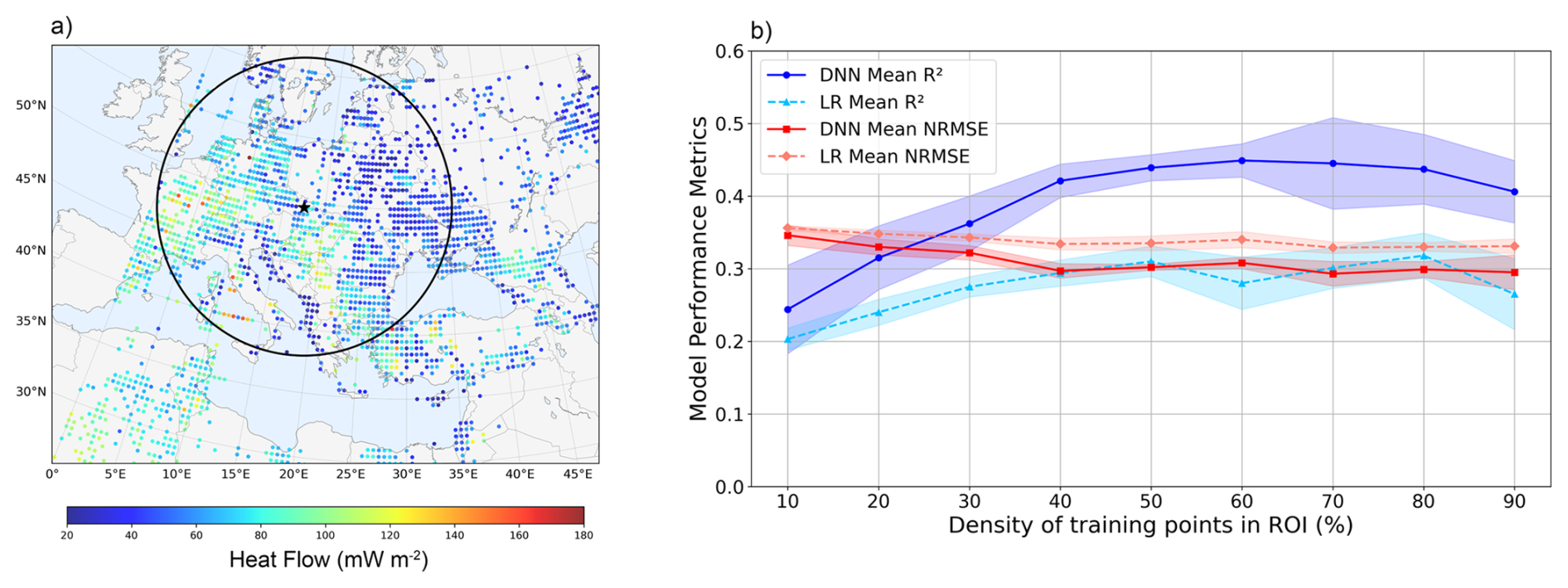
Figure 5 Performance of DNN and linear regression methods in experiments with different densities of ROI regions. (a) Test region where the black circle represents the ROI with maximum data density. (b) Performance comparison of DNN and linear regression under different training densities.

Experimental results (Fig. 5) demonstrate a pronounced positive correlation between data density and model performance. As training density within the ROI systematically increased from 10 % to 90 %, DNNs model predictive capability exhibited notable improvement: mean R² values increased from 0.24 ± 0.06 to approximately 0.41 ± 0.05, while mean NRMSE correspondingly decreased from 0.35 to a minimum of 0.31. The DNN model achieved relatively stable performance at training densities above 40 %, with R² values fluctuating between 0.41 and 0.45. In contrast, linear regression achieved lower R² values ranging from 0.20 to 0.31, with NRMSE remaining relatively stable around 0.33 ± 0.02 across all density levels. Analysis reveals that at the initial training density of 10 %, both models exhibited similar performance with minimal difference in predictive capability. However, as training density increased, the performance gap between DNN and linear regression progressively widened. At densities above 40 %, DNN achieved R² values approximately 0.10–0.15 higher than linear regression, demonstrating that the DNN model can effectively leverage nonlinear modelling capabilities trained on global datasets to capture complex geological and geophysical patterns. Linear regression, constrained by its linear assumptions, showed limited improvement potential regardless of increased local data availability, with NRMSE remaining relatively stable across all density levels. These characteristics demonstrate that DNN-based approach is well-suited for GHF prediction in data-scarce regions such as Antarctica.

4.4 Antarctic GHF Prediction

We applied our model to the entire Antarctic continent to yield an integrated spatial distribution of GHF (Fig. 6). Our results indicate that GHF values across the Antarctic continent range from 20 to 110 mW m⁻², with a mean value of 65.6 mW m⁻². In most cases, the spatial pattern of GHF uncertainty closely resembles that of the GHF predictions, with higher uncertainty magnitudes consistently localized in regions of elevated GHF.

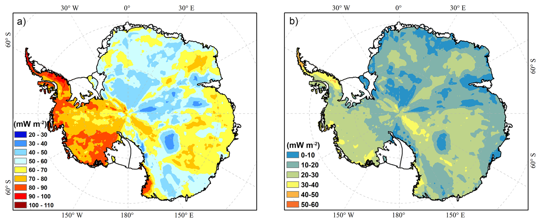
Figure 6 Predicted GHF distribution and associated uncertainty across Antarctica. (a) Mean GHF predictions from the five-fold cross-validation ensemble, ranging from 20 to 110 mW m⁻² (standard deviation). (b) Total predictive uncertainty derived from the Bayesian framework, ranging from 0 to 60 mW m⁻². Higher uncertainties are generally associated with regions of elevated GHF predictions.

To quantitatively assess the relationship between our predictions and existing models, we computed the spatial differences between our GHF map and six published estimates: Fox Maule et al. (2005), Martos et al. (2017), Shen et al. (2020), Lösing and Ebbing (2021), Stål et al. (2022), and Hazzard and Richards (2024). All models consistently show higher GHF in West Antarctica and uniformly low values in East Antarctica (Fig. 7). This fundamental contrast is primarily controlled by differences in tectonic history and lithospheric age (Boger, 2011; Veevers, 2012), with active tectonics and volcanism significantly influencing regional GHF in West Antarctica (Barletta et al., 2018). However, our model reveals a gradual increase in GHF across certain regions of East Antarctica. Although our results confirm that most of East Antarctica is characterized by stable low GHF, with minimum values located in the north of Belgica Subglacial Highlands, several regions of anomalously elevated GHF (> 70 mW m⁻²) are identified, including the Subglacial Lake Vostok region and the Vincennes Subglacial Basin.

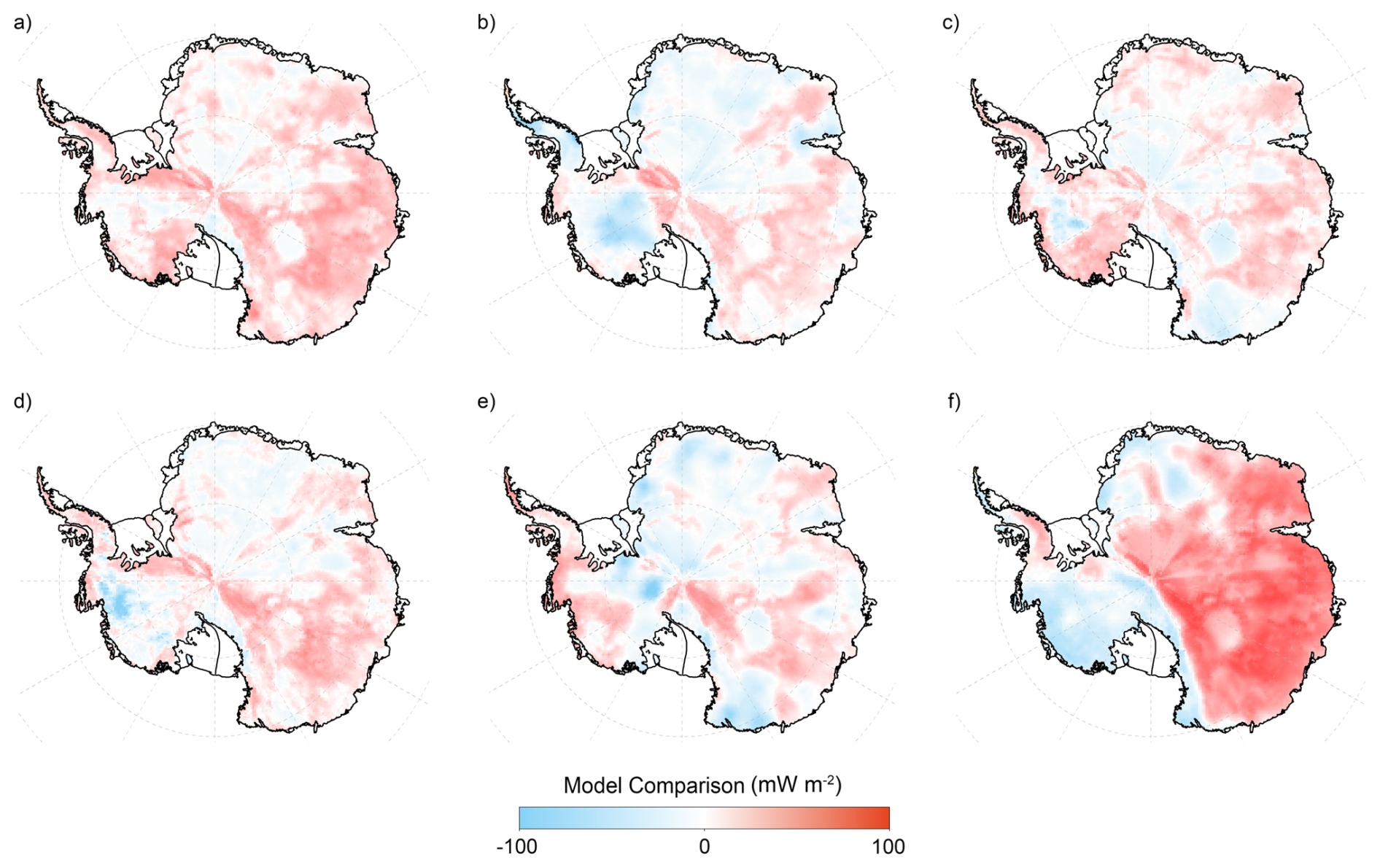
Figure 7 Spatial differences between our GHF predictions and six previously published models. (a) Ours – Shen et al. (2020). (b) Ours - Martos et al. (2017). (c) Ours – Lösing and Ebbing (2021). (d) Ours – Stål et al. (2021). (e) Ours - Fox Maule et al. (2017). (f) Ours – Hazzard and Richards, (2024). The maps are generated using the Antarctic Ice Shelf and Antarctic Coastline map of Mouginot et al. (2017) as a base map to define the continental extent and grounding line boundaries.

In terms of magnitude, our predicted values fall within a moderate range, lower than the peak values reported in magnetically based studies, yet higher than those derived from the seismic velocity method of Shen et al. (2020). The model of Martos et al. (2017) shows substantially higher values around the periphery of West Antarctica (reaching up to 240 mW m⁻²), with lower values in the interior. Our predictions are consistently lower in these extreme GHF regions, a discrepancy that likely reflects our data preprocessing approach, which removed outlier measurements exceeding 200 mW m⁻² to limit the influence of potentially anomalous values on model training. In contrast, the seismic-based model of Shen et al. (2020) shows higher coastal values and lower inland values, with continent-wide estimates not exceeding 90 mW m⁻², representing a more conservative thermal structure. Our model shows the closest agreement with Shen et al. (2020) in West Antarctica.

On a local scale, our model identifies elevated GHF anomalies in central East Antarctica, including the Subglacial Lake Vostok and the Vincennes Subglacial Basin, with predicted values locally exceeding 70 mW m⁻². The thermal anomaly in the Subglacial Lake Vostok region may indicate underlying magmatic or hydrothermal activity beneath the lake, potentially contributing to enhanced basal melting and meltwater generation (Artemieva, 2022). These findings support the emerging consensus that East Antarctica is not exclusively composed of a cold, uniform craton but rather harbors a more complex and heterogeneous thermal architecture (Shen et al., 2020).

4.5 Uncertainty Quantification

The results of the uncertainty quantification (UQ) derived from our Bayesian Neural Network framework are illustrated in Fig. 6. Following the decomposition approach described in Sect. 3.2, we evaluated the relative contributions of aleatoric and epistemic components to the total predictive uncertainty across the Antarctic continent.

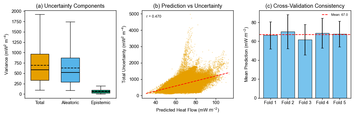
Figure 8 Uncertainty decomposition and cross-validation consistency analysis. (a) Distribution of uncertainty components across Antarctica. Aleatoric uncertainty constitutes the dominant fraction of total uncertainty, while epistemic uncertainty remains substantially lower, indicating that inherent observational variability rather than model limitations dominates predictive uncertainty. (b) Relationship between predicted GHF and total uncertainty, showing a positive correlation (r = 0.470). (c) Cross-validation consistency across five folds. Mean predictions show minimal variation between folds (overall mean = 67.0 mW m⁻²), with error bars representing standard deviations.

The distribution of uncertainty components (Fig. 8a) reveals that aleatoric uncertainty constitutes the dominant fraction of total uncertainty throughout the study region. The median aleatoric uncertainty (∼ 650 mW² m⁻⁴) substantially exceeds the median epistemic uncertainty (∼ 70 mW² m⁻⁴), indicating that inherent variability in heat flow observations and unresolved local geological heterogeneity represent the primary sources of predictive uncertainty. This finding suggests that the model has sufficient capacity and training data to capture the underlying patterns, while the irreducible observational noise and small-scale geological complexity impose fundamental limits on prediction accuracy.

We observed a moderate positive correlation (r = 0.47; Fig. 8b) between predicted GHF and total uncertainty, indicating that regions of high heat flow are systematically associated with greater predictive variance. This heteroscedastic pattern is geologically consistent: elevated GHF typically occurs in active tectonic settings (e.g., volcanic provinces and rift systems), where subsurface thermal regimes exhibit high spatial variability and logistical constraints often hinder dense data acquisition.

The consistency of predictions across the 5-fold cross-validation (Fig. 8c) further demonstrates the robustness of our modelling framework. The mean predictions show minimal variation between folds, with a cross-fold standard deviation of only 8.4 mW m⁻². This stability confirms that the model generalizes well to unseen data and that the uncertainty estimates are reproducible across different data partitions. Our hybrid architecture, which utilizes deterministic hidden layers coupled with a Bayesian output layer, represents a pragmatic trade-off between full Bayesian inference and computational efficiency. While this design facilitates uncertainty quantification, it implies that epistemic uncertainty is primarily captured via the final layer weights, which may lead to a conservative estimate of the total model uncertainty compared to a fully Bayesian treatment.

5 Discussion

5.1 Methodology Appraisal

We employed exponential distance weighting for volcano proximity features, assuming that thermal influence decays smoothly with distance according to a characteristic length scale. In reality, the spatial extent of volcanic thermal anomalies depends on factors including magma flux, crustal thermal conductivity, and time since emplacement – all of which vary substantially across different volcanic systems. Consequently, this simplified parameterization may not fully capture the heterogeneous thermal footprints of individual volcanic centres. While our VIF-based approach effectively mitigates multicollinearity, a pervasive issue in geoscientific modelling, it remains a purely statistical filter that overlooks the physical relevance of individual predictors. As a result, geologically significant variables may be excluded if they are highly redundant with retained features. Future iterations could incorporate physics-informed feature selection to better balance statistical rigor with domain expertise.

Compared with grid search and random search, PSO leverages swarm intelligence to navigate the parameter landscape more effectively. That said, computational cost remains a limitation: each PSO iteration requires training a complete neural network, making extensive hyperparameter searches time-consuming. Despite the superior accuracy of deep learning, its “black-box” nature often obscures the intuitive link between input features and physical mechanisms (Dramsch, 2020). We addressed this through cross-validation and rigorous uncertainty quantification, yet we advise caution when interpreting estimates in regions characterized by extreme data sparsity, where model extrapolations are less constrained.

Our Bayesian framework decomposes total predictive uncertainty into aleatoric and epistemic components, revealing that aleatoric uncertainty, arising from inherent observational variability and unresolved geological heterogeneity, constitutes the primary source of total uncertainty across Antarctica (Fig. 8a). This finding suggests that while our model architecture has sufficient capacity to capture underlying patterns, irreducible noise in heat flow observations and small-scale geological complexity impose fundamental limits on prediction accuracy (Fig. S14). Recent work by Al-Aghbary et al. (2025) demonstrates a promising approach to address this limitation. By applying unsupervised clustering to partition geophysical observables into homogeneous subsets and training dedicated local expert models within a Mixture-of-Experts (MoE) framework, they achieved substantial reductions in aleatoric uncertainty while maintaining stable epistemic uncertainty. This cluster-specific modelling strategy offers a compelling direction for future improvement of Antarctic GHF predictions, particularly given the pronounced geological heterogeneity between tectonically active West Antarctica and stable East Antarctic cratons. Implementing this cluster-based approach could potentially reduce the elevated uncertainties observed in our predictions.

5.2 Spatial Representativeness and Data Limitations

A fundamental challenge in continental-scale GHF modelling lies in the spatial representativeness of in-situ point measurements. Individual determinations sample highly localized thermal regimes that may not be representative of broader regional averages, particularly in geologically heterogeneous environments. This issue is especially acute in Antarctica, where sparse observations must represent vast areas spanning thousands of square kilometres per grid cell. Studies from West Antarctica have documented substantial local variations in geothermal heat flow over distances of tens of kilometres (Fisher et al., 2015; Schroeder et al., 2014), reflecting heterogeneous distributions of radiogenic heat-producing elements, variable crustal thickness, and localized volcanic or hydrothermal activity. When training data consist predominantly of single measurements per region, machine learning models cannot distinguish whether these observations represent typical regional conditions or localized anomalies. Our uncertainty quantification framework captures prediction uncertainty conditional on the training data, but cannot account for systematic biases arising from unrepresentative sampling.

Additionally, the quality of available Antarctic heat flow measurements presents additional concerns. Most measurements derive from temperature gradients within ice columns or shallow sediments rather than bedrock boreholes, introducing uncertainties related to thermal non-equilibrium, paleoclimatic temperature perturbations, and englacial heat sources from ice deformation. The limited number of high-quality bedrock measurements means that our model is effectively extrapolating from a sparse and potentially biased training dataset. Moreover, borehole-derived GHF estimates in Antarctica are often higher than geophysical model predictions and subject to limitations of one-dimensional thermal assumptions (Mony et al., 2020; Talalay et al., 2020), which further complicates model validation efforts.

5.3 Future Directions

Several prospective avenues merit exploration. First and foremost, the acquisition of additional high-quality field GHF measurements remains essential, particularly in geologically complex regions of East Antarctica where current data coverage is sparse. A deeper understanding and quantitative assessment of subglacial GHF in Antarctica necessitates refined analysis of crustal geological characteristics and their inherent complexity. Conventional studies, constrained by insufficient observational heat production data, have often oversimplified or neglected these factors. However, recent research demonstrates that crustal heat generation plays a non-negligible role in the modelling of subglacial heat flow, driving interdisciplinary integration between glaciology (including observations and modelling) and subglacial geology (Li and Aitken, 2024; Stål et al., 2024). At the same time, Antarctic bedrock boreholes face great challenges, with measurements now available only in a few ice-free or subglacial regions. These data mainly reflect localized temperature structures and are highly uncertain because most boreholes fail to reach solid bedrock and estimate heat flow only from temperature gradients within ice caps or loose sediments, which are susceptible to climate forcing, hydrothermal circulation, and ice dynamics (Fisher et al., 2015). Therefore, direct validation of data becomes a substantial bottleneck in current research.

Recent advancements in Interpretable Machine Learning (IML) and Explainable AI (XAI) (Gunning and Aha, 2019; Murdoch et al., 2019) have opened new avenues for deciphering the “black-box” nature of deep learning models. While deep learning outperforms conventional simplistic models in predictive accuracy, its opaque decision-making process hinders intuitive understanding of feature importance and directional influences (Dramsch, 2020). To bridge this gap, validating the compatibility of model mechanisms with current geologic information can be beneficial in boosting their credibility, while offering new routes for studying and interpreting complicated linkages in geoscientific data. By understanding the process of machine learning models, we can get insights into how diverse input features interact and influence geoscientific events, including relationships that may be difficult to discover through conventional analyses (Ham et al., 2023; Jiang et al., 2024). One promising route for improving the model is to incorporate physical constraints into the activation function design, which enhances the physical consistency of the outputs. Further development of this technique is anticipated. In addition, a posteriori interpretation of model outputs in conjunction with interpretability assessments is also crucial.

6 Conclusions

In this study, we present an integrated framework combining PSO-optimized deep neural networks with Bayesian uncertainty quantification for predicting Antarctic GHF. Through regional density experiments, we found that our model significantly outperforms linear regression in terms of prediction accuracy and nonlinear mapping capacity, particularly in data-constrained environments. The resulting GHF distribution reveals a pronounced East-West dichotomy. Elevated heat flow anomalies are concentrated along the coastal margins of West Antarctica, primarily driven by active lithospheric extension and tectonic activity. Notably, our model predicts elevated GHF values in East Antarctica compared to previous studies, suggesting that the East Antarctic Shield may not be as uniformly cratonic or thermally stable as formerly assumed. Furthermore, uncertainty decomposition reveals that aleatoric components dominate the total predictive variance, highlighting the fundamental limits on predictability imposed by inherent observational noise and unresolved small-scale geological heterogeneity. Future research should prioritize the acquisition of high-quality borehole measurements in data-sparse regions and the integration of physics-informed constraints to enhance model interpretability and geophysical fidelity.