The effect of the present-day imbalance on schematic and climate forced simulations of the West Antarctic Ice Sheet collapse

Recent observations reveal that the West Antarctic Ice Sheet is rapidly thinning, particularly at its two largest outlet glaciers, Pine Island Glacier and Thwaites Glacier, while East Antarctica remains relatively stable. Ice sheet model projections over the next few centuries give a mixed picture, some ice sheet models forced by climate models project mass gain by increased surface mass balance, while most models project moderate to severe mass loss by increasing ice discharge. In this study, we explore the effect of present-day ice thickness change rates on forced future simulations of the Antarctic Ice Sheet using the Community Ice Sheet Model (CISM). We start with a series of schematic, uniform ocean temperature perturbations in the Amundsen Sea Embayment (ASE) to probe the sensitivity of the modelled present-day imbalance to ocean warming. We then apply ocean and atmospheric forcing from seven datasets produced by five Earth System Models (ESMs) from the CMIP5 and CMIP6 ensemble to simulate the Antarctic Ice Sheet from 2015 to 2500. The schematic experiments suggest the presence of an ice-dynamical limit; Thwaites Glacier (TG) does not collapse in these experiments (i.e., with accelerated deglaciation leading to considerable grounded ice mass loss) before ∼2100 without more than 2° of ocean warming. Meanwhile, the maximum rate of Global Mean Sea Level rise (GMSLr) from the ASE during the collapse increases linearly with ocean temperature, indicating that while earlier collapse timing shows diminishing returns, the rate of sea-level rise keeps on intensifying with stronger forcing. The relative importance of including the observed present-day mass loss rates decreases for larger (ocean) warming under climate forcing, and decreases over time. For the East Antarctic Ice Sheet on shorter timescales (until 2100), adding the present-day observed mass change rates doubles its global mean sea level rise contribution. On longer timescales (2100–2500), the effect of the present-day observed mass change rates is smaller. Thinning of the West Antarctic Ice Sheet induced by the present-day imbalance is partly compensated by present-day ice sheet thickening of the East Antarctic Ice Sheet over the coming centuries, which persists in our simulations. These deviations are overshadowed by the mass losses induced by the projected ocean warming.

1 Introduction

The latest IPCC estimate of the Antarctic Ice Sheet (AIS) contribution to global mean sea level (GMSL) rise ranges from 0.03 m (SSP1-1.9, low end of the likely range) to 0.34 m (SSP5-8.5, high end of the likely range) in 2100 (Fox-Kemper et al., 2021). This is an assessment based on ice sheet models, which simulate the future behaviour of the AIS. The uncertainty in modelled ice sheet contribution to sea level from the AIS until 2100 is relatively low because the major floating ice shelves keep the grounded ice sheet currently in place (Van De Wal et al., 2022), but increases rapidly after 2100 because non-linear processes could accelerate mass loss significantly (Fox-Kemper et al., 2021; Payne et al., 2021; DeConto et al., 2021). It is argued that the main contributors to Antarctic mass loss uncertainty in the long term (e.g. after 2100) are the choice of ice flow model and the choice of the Earth System Model (ESM) used as ocean and atmospheric forcing (Pattyn and Morlighem, 2020; Aschwanden et al., 2021).

Both ice flow models and ESMs have grown in number over the past decades. This has increased the capability to quantify the uncertainty related to the choice of the ice sheet model and to the choice of ESM forcing. The Ice Sheet Model Intercomparison for CMIP6 (ISMIP6, Nowicki et al., 2016, 2020) exemplifies multi-model ensemble simulations of the AIS and state-of-the-art quantification of different sources of uncertainty in sea level rise projections. Seroussi et al. (2023) show that until 2100, the choice of ice sheet model (which encompasses all modelling choices, including the momentum balance approximation, resolution, initialization method and parameterizations) is the dominant source of uncertainty of projected GMSL from the AIS, with a growing uncertainty caused by the choice of ESM forcing over time. This study shows large geographic differences: for example, the variance associated with the ice sheet model is large for Thwaites Glacier (TG) and Pine Island Glacier (PIG), which at present-day exhibit the largest ice thinning rates according to recent observations (Smith et al., 2020), and small for the MacAyeal and Whillans glaciers. In a follow-up study, Seroussi et al. (2024) show that the choice of ice flow model remains the largest source of uncertainty until 2300, with ESM forcing as second largest contributor. Among other model differences, a main difference is the method used to simulate the present-day state of the AIS, here referred to as the initialization method.

To obtain a good model representation of the present-day configuration of the AIS it is necessary to do a model initialization. In an initialization, modellers often include the observed ice thickness and/or the observed ice surface velocities as target variables for the model to match (Winkelmann et al., 2011; Pollard and Deconto, 2012; Greve and Blatter, 2016; Quiquet et al., 2018; Lipscomb et al., 2019; Berends et al., 2021, 2022). In these methods, the ice sheet model parameters are adjusted by comparing modelled and observed ice surface velocities while either imposing observed ice thickness and/or ice surface velocities (the so-called Data Assimilation method) or by doing a forward run with either historical or present-day forcing (the spin-up method). This process can lead in some cases to nonzero ice thickness change rates, or drift, when the model is run forward in time, even without external climate forcing. All three studies by Rosier et al. (2021), Bett et al. (2024) and Rosier et al. (2025) state that it is impossible to obtain a perfect fit between observed and modelled ice thickness, ice surface velocities, and mass change rates simultaneously because the three datasets are not mutually consistent (Morlighem et al., 2011).

To get the modelled ice sheet to exhibit a mass change rate, ideally also close to observations, a historical forcing scenario can be used (Reese et al., 2023; Coulon et al., 2024; Klose et al., 2024). Recently, Van Den Akker et al. (2025) developed a method to incorporate the observed mass change rates in this spin-up initialization, in which the gridded observed mass change rates are subtracted from the mass transport equation. In this way, the resulting modelled ice sheet can start future simulations immediately from the observed imbalance. This circumvents the need for a historical simulation and forcing over the near-present period. Van Den Akker et al. (2025) show that initialization with the present-day observed mass change rates in two ice-sheet models always leads to an unforced collapse (i.e., without additional ocean or atmospheric warming) of the West Antarctic Ice Sheet (WAIS), starting with Thwaites Glacier (TG) and Pine Island Glacier (PIG). The rapid collapse phase typically begins after a period of 500–2000 years of slow retreat. However, that study only showed simulations with a sustained present-day climate; it did not investigate how the present-day imbalance affects simulations that include future climate change (hereafter labelled as “forcing”).

In this study, we focus on forced simulations of the Antarctic Ice Sheet, first using schematic ocean warming, and secondly ocean temperature and SMB anomalies from five ESMs from the CMIP5 and CMIP6 ensembles following either the SSP1-2.6, SSP5-8.5, RCP1-26 or the RCP 5-85 scenario. The schematic forcing consists of a targeted (e.g. only at TG and PIG) sudden uniform ocean warming up to 2°. The ESM forcing used in this study has also been used as forcing for the ISMIP6 Antarctic Ice Sheet study in Seroussi et al. (2024). These anomalies serve as input to long-term future simulations from 2015 to 2500, to capture the longer-term effects of climate change on the mass of the ice sheet. We use two initializations of the Antarctic ice sheet to start our future simulations, namely with and without the observed mass change rates. Hence, the latter starts from steady-state. With these simulations we investigate the importance for the future evolution of the Antarctic Ice Sheet (AIS) of the current imbalance of the AIS compared to projected future changes in ocean temperature and SMB. For example, do they add up linearly, or does the present-day imbalance influence the forced deglaciation of the WAIS? In Sect. 2, we introduce the Community Ice Sheet Model, and we discuss the general initialization procedure and the oceanic and atmospheric ESM forcings used. In Sect. 3, we show the results of the future projections. Section 4 contains the discussion, followed by conclusions in Sect. 5.

2 Methods

2.1 Community Ice Sheet Model (CISM)

The Community Ice Sheet Model (CISM, Lipscomb et al., 2019, 2021) is a thermo-mechanical higher-order ice sheet model, which is part of the Community Earth System Model version 2 (CESM2, Danabasoglu et al., 2020). Earlier applications of CISM to Antarctic Ice Sheet retreat can be found in Lipscomb et al. (2021), Berdahl et al. (2023), and Van Den Akker et al. (2025, 2026). The variables and constants used in the text and equations below are listed in Tables S1 and S2 in the Supplement.

We run CISM with a vertically integrated approximation to the momentum balance, the Depth Integrated Viscosity Approximation (DIVA) (Goldberg, 2011; Lipscomb et al., 2019; Robinson et al., 2022):

$$\begin{array}{}\text{(1)}& {\displaystyle }\begin{array}{rl}{\displaystyle \frac{\partial }{\partial x}}& \left(\mathrm{2}\underset{\mathrm{¯}}{\mathit{\eta }}H\left(\mathrm{2}{\displaystyle \frac{\partial \underset{\mathrm{¯}}{u}}{\partial x}}+{\displaystyle \frac{\partial \underset{\mathrm{¯}}{v}}{\partial y}}\right)\right)\\ & +{\displaystyle \frac{\partial }{\partial y}}\left(\underset{\mathrm{¯}}{\mathit{\eta }}H\left({\displaystyle \frac{\partial \underset{\mathrm{¯}}{u}}{\partial y}}+{\displaystyle \frac{\partial \underset{\mathrm{¯}}{v}}{\partial x}}\right)\right)-{\mathit{\tau }}_{\mathrm{b},x}={\mathit{\rho }}_{\mathrm{i}}gH{\displaystyle \frac{\partial s}{\partial x}}\end{array}\text{(2)}& {\displaystyle }\begin{array}{rl}{\displaystyle \frac{\partial }{\partial x}}& \left(\underset{\mathrm{¯}}{\mathit{\eta }}H\left({\displaystyle \frac{\partial \underset{\mathrm{¯}}{u}}{\partial y}}+{\displaystyle \frac{\partial \underset{\mathrm{¯}}{v}}{\partial x}}\right)\right)\\ & +{\displaystyle \frac{\partial }{\partial y}}\left(\mathrm{2}\underset{\mathrm{¯}}{\mathit{\eta }}H\left(\mathrm{2}{\displaystyle \frac{\partial \underset{\mathrm{¯}}{v}}{\partial v}}+{\displaystyle \frac{\partial \underset{\mathrm{¯}}{u}}{\partial x}}\right)\right)-{\mathit{\tau }}_{\mathrm{b},y}={\mathit{\rho }}_{\mathrm{i}}gH{\displaystyle \frac{\partial s}{\partial y}}\end{array}\end{array}$$

in which $\underset{\mathrm{¯}}{\mathit{\eta }}$ is the depth-averaged viscosity, H the ice thickness, $\underset{\mathrm{¯}}{u}$ and $\underset{\mathrm{¯}}{v}$ respectively the depth-averaged ice velocities in the x and y direction, ρ_i the density of glacial ice and s the surface height above sea level. Basal friction, which appears as τ_b,x and τ_b,y in Eqs. (1) and (2), can be parameterized in several ways. In this study we use a regularized Coulomb sliding law first suggested by Schoof (2005) and confirmed with laboratory experiments by Zoet and Iverson (2020):

$$\begin{array}{}\text{(3)}& {\mathit{\tau }}_{\mathrm{b}}=\mathit{\beta }{u}_{\mathrm{b}}=C_{\mathrm{c}}N{\left({\displaystyle \frac{u_{\mathrm{b}}}{u_{\mathrm{b}}+u_{\mathrm{0}}}}\right)}^{\frac{\mathrm{1}}{m}}\end{array}$$

where C_c is a unitless parameter in the range [0,1] controlling the strength of the regularized Coulomb sliding, u_b the ice basal velocities and u₀ and m are free parameters. The effective pressure N is estimated according to Leguy et al. (2014) and Leguy et al. (2021):

$$\begin{array}{}\text{(4a)}& N={\mathit{\rho }}_{\mathrm{i}}gH{\left(\mathrm{1}-{\displaystyle \frac{H_{\mathrm{f}}}{H}}\right)}^p\end{array}$$

where the flotation thickness H_f is given by

$$\begin{array}{}\text{(4b)}& H_{\mathrm{f}}=\left(\mathrm{0},-{\displaystyle \frac{{\mathit{\rho }}_{\mathrm{w}}}{{\mathit{\rho }}_{\mathrm{i}}}}b\right)\end{array}$$

with ρ_i for the density of glacial ice, ρ_w the density of ocean water, g the gravitational acceleration and b the height of the bedrock. In Eq. (4a), p (a parameter in the range [0,1]) controls the decrease in effective pressure of ice resting on bedrock below sea level. Setting p=1 implies that, at the modelled grounding lines, the overburden pressure at the ice base is completely balanced by the ocean pressure, and N approaches zero. In this study we use p=1, assuming full connectivity of the subglacial hydrological network with the ocean. This scheme, proposed by Leguy et al. (2014), accounts for basal water pressure (which reduces N) only near grounding lines and not in other parts of the ice sheet; thus the effective pressure equals ice overburden for most of the ice sheet.

Since C_c is poorly constrained by theoretical considerations and observations, we use it as a spatially variable tuning parameter. We tune the logarithm of C_c using a nudging method, i.e. a 10 kyr simulation with present-day forcing in which the modelled ice sheet is allowed to evolve freely while slowly changing C_c based on an observational thickness target (Lipscomb et al., 2021; Pollard and Deconto, 2012):

$$\begin{array}{}\text{(5a)}& {\displaystyle }\begin{array}{rl}{\displaystyle \frac{\mathrm{d}{C}_{\mathrm{l}}}{\mathrm{d}t}}& =-\left({\displaystyle \frac{H-H_{\text{obs}}}{H_{\mathrm{0}}\mathit{\tau }}}\right)-{\displaystyle \frac{\mathrm{2}}{H_{\mathrm{0}}}}{\displaystyle \frac{\mathrm{d}H}{\mathrm{d}t}}\\ & -{\displaystyle \frac{r}{\mathit{\tau }}}(C_{\mathrm{l}}-C_{\text{lr}})+{\displaystyle \frac{L^{\mathrm{2}}}{\mathit{\tau }}}\mathrm{\Delta }{C}_{\mathrm{l}}\end{array}\text{(5b)}& {\displaystyle }{C}_{\mathrm{l}}=\log \left(C_{\mathrm{c}}\right)\end{array}$$

In Eq. (5a), H₀, τ, r and L are scaling constants, used to adjust the relative weights of the different terms. Increasing/decreasing H₀ makes the optimalization less/more sensitive to ice thickness errors; increasing/decreasing τ makes the changes in C_l per timestep smaller/larger, increasing/decreasing r draws C_l more/less to the relaxation target C_l; and increasing/decreasing L results in a smoother/spikier 2D pattern of optimized C_l. Their values were tested and chosen to represent AIS thickness and surface velocities well, with minimal drift. Table S2 shows their values.

The logarithmic relaxation target C_lr is a 2D field that penalizes very high and low values of C_c. It is based on elevation, with lower values at low elevation where soft marine sediments are likely more prevalent, following Winkelmann et al. (2011). We chose targets of 0.1 for bedrock below −700 m a.s.l. and 0.4 for 700 m a.s.l., with linear interpolation in between, based on Aschwanden et al. (2013). The motivation for this is that lower elevations deglaciate earlier and therefore have more softer marine till relative to higher elevated bedrock, since they likely were deglaciated more in the past compared to regions with higher bedrock. The parameterization and associated values used to represent marine sediments in Aschwanden et al. (2013), which rely solely on bedrock elevation, are challenged by the more recent findings of Li et al. (2022), who show that the likelihood of marine sediment does not directly correlate with bedrock height. Incorporating the likelihood map of Li et al. (2022) into CISM and analysing the influence of marine sediments on marine-based ice sheets is beyond the scope of this study, but represents a promising direction for future work.

The last term on the RHS of Eq. (5a) is new compared to Lipscomb et al. (2021) and Van Den Akker et al. (2025, 2026) and is introduced to smooth the pattern of optimized C_c by suppressing large spatial gradients. Smoothing also reduces the model drift as a local grounding line position can no longer be pinned by one grid box with high basal friction.

Basal melt rates (BMR) are calculated using a quadratic relation with a sub-shelf thermal forcing during the initialization and the forced simulations:

$$\begin{array}{}\text{(6)}& \text{BMR}={\mathit{\gamma }}_{\mathrm{0}}{\left({\displaystyle \frac{{\mathit{\rho }}_{\mathrm{w}}{c}_{\text{pw}}}{{\mathit{\rho }}_{\mathrm{i}}{L}_{\mathrm{f}}}}\right)}^{\mathrm{2}}\left(\right[{\text{TF}}_{\text{base}}+\mathit{\delta }T,\mathrm{0}]{)}^{\mathrm{2}}\end{array}$$

in which the baseline thermal forcing, TF_base, is the difference between the melting point and the ocean temperature at the base of the modelled ice shelf, and δT a local correction temperature. The thermal forcing is derived from a climatology based on Southern Ocean observations of the past few decades (Jourdain et al., 2020). This basal melt parameterization was developed and tested by Jourdain et al. (2020) and Favier et al. (2019) with the purpose of modelling present-day Antarctic basal melt rates. The quadratic relationship between thermal forcing and basal melt rates reflects a positive feedback. As the ice shelf melts, freshwater is added to the cavity, which is more buoyant than the saltier ocean water. This causes the sub-shelf meltwater plume to rise faster, and through erosion and upwelling of new warm ocean water, the basal melt rates will increase. Equation (6) parameterizes this feedback to a reasonable approximation for present-day basal melt rates, but it is unknown how well it simulates basal melt rates for several degrees of (future) ocean warming.

The basal melt rates are tuned through the local correction temperature δT such that the floating ice thickness matches as closely as possible the thickness observations of Morlighem et al. (2020) following a similar procedure as for friction (Eq. 5):

$$\begin{array}{}\text{(7)}& \begin{array}{rl}{\displaystyle \frac{\mathrm{d}\left(\mathit{\delta }T\right)}{\mathrm{d}t}}& =T_{\mathrm{s}}\left[\left({\displaystyle \frac{H-H_{\text{obs}}}{H_{\mathrm{0}}\mathit{\tau }}}\right)+{\displaystyle \frac{\mathrm{2}}{H_{\mathrm{0}}}}{\displaystyle \frac{\mathrm{d}H}{\mathrm{d}t}}\right]\\ & +{\displaystyle \frac{(T_{\mathrm{r}}-\mathit{\delta }T)}{\mathit{\tau }}}+{\displaystyle \frac{L^{\mathrm{2}}}{\mathit{\tau }}}\mathrm{\Delta }\mathit{\delta }T\end{array}\end{array}$$

in which T_s is the temperature scale of the nudging method (0.5 K in this study). This tuning increases (decreases) the local correction temperature δT in grid cells where the modelled ice shelf is too thick (thin), increasing (decreasing) the basal melt rates. The tuning includes a relaxation target T_r, being 0, to penalize large deviations from the dataset of Jourdain et al. (2020). The melt sensitivity γ₀ is chosen to be 3.0×10⁴ m yr⁻¹, which was used in Lipscomb et al. (2021), and Van Den Akker et al. (2025, 2026) to obtain basal melt rates in agreement with observations and a shelf average δT close to zero in the Amundsen Sea Embayment, where currently the largest ice shelf melt rates are observed (Adusumilli et al., 2020). The last term is added, as for the C_c optimalization in Eq. (5), to suppress large spatial variations in the optimized ocean temperature perturbation field, as large differences of several degrees between adjacent grid cells are physically implausible.

To prevent abrupt jumps in modelled quantities at the grounding line (such as basal friction and basal melt), we use a grounding line parameterization from Leguy et al. (2021):

$$\begin{array}{}\text{(8)}& f_{\text{float}}=-b-{\displaystyle \frac{{\mathit{\rho }}_{\mathrm{i}}}{{\mathit{\rho }}_{\mathrm{w}}}}H\end{array}$$

When f_float is positive it is equal to the distance between the ice shelf base and the ocean floor and hence, the ice is floating. When f_float is negative, it can be interpreted as the ice thickness change needed for the ice column to become floating. The variable f_float is used to compute the floating fraction as a percentage of grid cell area by bilinearly interpolating its value from cell vertices to the cell areas scaled to the cavity thickness (Leguy et al., 2021). The grounded and floating fraction of a cell are then used to scale basal friction and basal melting. For the basal melting, this is referred to as the Partial Melt Parameterization (PMP, see Leguy et al., 2021).

Schematic tests by Seroussi and Morlighem (2018) showed that applying basal melt in proportion to the floating area fraction can lead to an overestimation of grounding line retreat rates; they therefore discouraged the use of PMPs. However, Leguy et al. (2021) conducted similar schematic tests with CISM and found that using a PMP reduced CISM's sensitivity to grid resolution more than the No-Melt Parameterization (NMP) recommended by Seroussi and Morlighem. In more realistic AIS applications of CISM, Lipscomb et al. (2021) found that the PMP produced a moderate sensitivity of grounding line migration rates to grid resolution, lower than the sensitivities to basal melt rate and basal friction parameterizations. These results suggest that the optimal GLP is model-dependent and that for CISM, 4 km grid resolution using a PMP is sufficient for modelling continental-scale ice sheets on multi-century timescales.

We run CISM on a uniform 4 km grid, justified below. using the grounding line parameterization from Leguy et al. (2021) which scales the basal sliding and melt rate proportionally to its grounded and floating area fraction respectively in elements that contain the modelled grounding line. Doing so, Leguy et al. (2021) showed that this resolution is adequate to capture grounding line dynamics using CISM and idealized marine ice sheet experiments, Lipscomb et al. (2021) showed that this resolution in combination with the scaling reduces the model result's grid resolution dependency when modelling the AIS.

There are several calving laws in the literature e.g. Yu et al. (2019), Wilner et al. (2023), Greene et al. (2022) and specifically for Greenland (Choi et al., 2018). However, there is no agreed-upon best approach to Antarctic calving (Levermann et al., 2012), and most calving laws struggle to reproduce the observed calving front at multiple locations simultaneously without adjusting local parameters (Amaral et al., 2020). We therefore choose to apply a simple no-advance calving scheme, preventing the calving front from advancing beyond the observed present-day location. The ice shelf front can retreat only through ice shelf thinning. This implies that the ice shelf front can only retreat when the basal melt rates increase greatly and become sufficiently high to remove floating ice upstream of the present-day calving front. In practice, this means that the calving front will only retreat when the basal melt rates are increased greatly, and for present-day conditions, this means that the calving front position is fixed at its observed location. This is a conservative approach, ignoring the possibility of calving-front retreat through shelf thinning or of shelf collapse by hydrofracturing. The implementation of a more physically-based calving law in CISM is the topic of ongoing research.

2.2 Initializations

We perform initializations with or without incorporating the observed present-day mass change rates, hence leading to a transient and equilibrium initial state, respectively. For the equilibrium initialization, C_c and δT are tuned using Eqs. (5) and (7) until the modelled ice sheet is in equilibrium, thus $\partial H/\partial t=\mathrm{0}$, given by

$$\begin{array}{}\text{(9)}& {\displaystyle \frac{\partial H}{\partial t}}=-\mathrm{\nabla }\left(\stackrel{\mathrm{‾}}{u}H\right)+B\end{array}$$

In Eq. (9), $\underset{\mathrm{¯}}{u}$ is the vertical mean velocity, and B the sum of the basal and SMBs. For the transient initialization, C_c and δT are tuned using mass conservation complemented by the present-day observed mass change rates as was done by Van Den Akker et al. (2025), using

$$\begin{array}{}\text{(10)}& {\displaystyle \frac{\partial H}{\partial t}}=-\mathrm{\nabla }\left(\stackrel{\mathrm{‾}}{u}H\right)+B-{\left.{\displaystyle \frac{\partial H}{\partial t}}\right|}_{\text{obs}}\end{array}$$

in which the last term, the pseudo-flux, is the observed mass change from Smith et al. (2020). By subtracting this observed mass change, mass is added during the initialization where thinning is observed. After the initialization and for normal forward simulations, this pseudo-flux is removed, so that model simulations start with an imbalance and a thinning rate closely matching the observed thinning rates. Both initializations are run for 10 kyr, which proved to be long enough to reach a (thermal) equilibrium. We evaluate both initializations by comparing to observations of ice thickness (Morlighem et al., 2020), ice surface velocities (Rignot et al., 2011), total basal melt fluxes (Adusumilli et al., 2020; Rignot et al., 2013) and by evaluating their model drift. We test the drift by running forward for 1000 years (i.e., to the year 3015) without additional forcing with respect to present-day conditions, with the optimized parameters (e.g. δT and C_c in Eqs. 5 and 7) kept constant, and continuing to add the observed mass changes for the transiently initiated model state as described by Eq. (10). This is a time scale longer than our period of interest, which runs only to 2500, thus for 485 years. The resulting drift, shown in Figs. S1 and S2 in the Supplement, results in a WAIS change in IVAF over 1000 years of 0.5 % for the transient initialization and approximately 0 % for the equilibrium initialization. For the whole AIS, the model drift in the transient initialization is 0.05 % of the IVAF and −0.05 % for the equilibrium initialization. These results ensure that we can attribute any major changes in ice sheet mass to the applied forcing and not to model drift. Figure S3 in the Supplement shows the evolution of the average temperature during the initialization: it flattens out at 10 kyr, indicating that the ice sheet has reached thermal equilibrium.

2.3 Idealized schematic warming scenarios

To assess how sensitive the simulations starting from the transient initialization are to imposed ocean warming, and to compare this with the sensitivity of simulations starting from the equilibrium initialization, we conduct a set of idealized experiments in which ocean temperatures in the ASE region are systematically increased after initialization.

2.4 ESM-forced future projections

We first test the sensitivity of the two initializations to schematic ocean warming by conducting 11 idealized experiments with sudden and sustained warming, only in the ASE region shown in Fig. S4 in the Supplement. We raise the ocean temperature, which appears as the sum TF_base+δT in Eq. (6), from 0 to 2 K with steps of 0.2 K. Each experiment is run for 1000 years to allow for a possible WAIS collapse.

We then perform two sets (i.e. starting from the transient and starting from the equilibrium initialization) of simulations for each of the seven forcing datasets produced by the five different ESMs, introduced in the next section. We timestamp the end of our initialization at 2015 based on the observational datasets used to calibrate the model (Smith et al., 2020; Morlighem et al., 2020; Rignot et al., 2011). We then run CISM forward for 485 years to 2500. The seven forcing datasets from five different ESMs span the period 1995–2100, with four ESMs continuing until 2300 and one where the input forcing to the ESM was repeated from the late 21st century onwards. For the last 200 years of the simulations, we fix the thermal forcing and SMB anomalies at the last datapoint year (2300). We consider the whole continent in our analysis, but focus on areas with large changes and potentially large sea level contributions, like the Amundsen Sea Embayment, the Filchner-Ronne basin, and the Ross basin. Those areas are shown in Fig. S4.

We use the same set of ocean and SMB forcings as Seroussi et al. (2024). These forcings stem from seven ESM simulations from the CMIP5 and CMIP6 ensemble. Two models from the CMIP5 ensemble were selected by Barthel et al. (2020): the Community Climate Model (CCSM4) and the Hadley Centre Global Environment Model (HadGEM2-ES), with respective Equilibrium Climate Sensitivities (ECS) of 2.9 and 4.6 K (Meehl et al., 2020). Additionally, two CMIP6 participating models are used: the Community Earth System Model (CESM2) and the UK Earth System Model (UKESM), with ECS of respectively 5.2 and 5.3 K (Meehl et al., 2020). The Norwegian Earth System Model (NorESM, with an ECS of 2.5 K as reported by Meehl et al., 2020) was used as a reference run in the ISMIP6 ensemble and will be used in this study as well. The models HADGEM2-ES, CESM2 and UKESM have a climate sensitivity to doubling of CO₂ concentrations at the upper end of the 90 % confidence interval in the IPCC-AR6 report (Meehl et al., 2020). More information on the selection of these ESM forcings can be found in Barthel et al. (2020) and Seroussi et al. (2024).

The ocean forcings from the ESMs are applied similar to the thermal forcing TF_base in Eq. (6). For this set of simulations, cavity-resolving ocean models were not available among the CMIP5 and CMIP6 ensembles. Therefore, the ocean thermal forcing from the ESMs is interpolated into the ice shelf cavities following Jourdain et al. (2020). First, a marine connection mask is generated, marking cells with subzero topographic paths to the open ocean. Next, empty cells adjacent to filled ones and connected to the ocean are identified,. These cells are then filled with the average of neighboring filled values. Any empty cells below the new fill may remain if the local bedrock is deeper than in adjacent columns. In those cases, the thermal forcing is linearly extrapolated using a depth-dependent freezing point correction with a temperature coefficient of $\mathrm{7.64}\times {\mathrm{10}}^{-\mathrm{4}}$ K m⁻¹ from Beckmann and Goosse (2003). The last year (2300) of all 7 oceanic forcings, including the extrapolation below present-day grounded ice, relative to TF_base, are shown in Fig. 1.

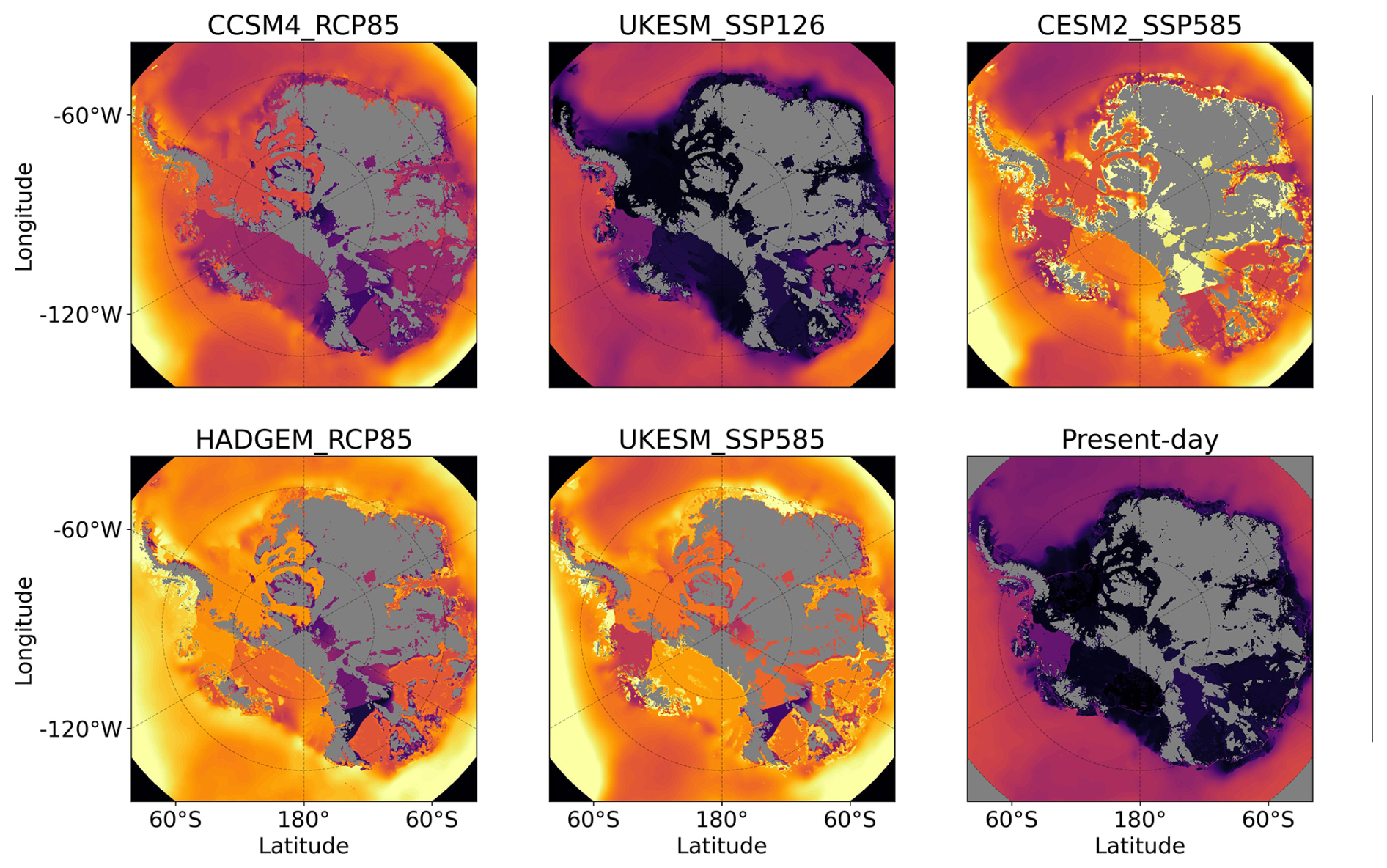
Figure 1 Thermal forcing (TF_base+δT in Eqs. 6 and 7) from the five ESMs used. Thermal forcing averages for the year 2300 (except the present-day) are shown for a depth of −500 m. Cells with bedrock above sea level are shown in grey. The simulations from NorESM run until 2100 and are shown in Fig. S8.

The computed ocean thermal forcing dataset has 30 layers with a vertical resolution of 60 m and extends down to 1770 m below sea level. The thermal forcing at the ice-shelf base is linearly interpolated between vertically adjacent ocean layers. If the ice lies below the lowest ocean layer, which can occur in deep troughs beneath the Filchner-Ronne and Amery shelves, the thermal forcing is extrapolated from the lowest layer using the depth-dependent freezing point temperature coefficient from Beckmann and Goosse (2003).

Figure 2 shows the SMB anomalies of seven simulations of the five ESMs. Large differences in magnitude are visible, with NorESM_RCP26 and NorESM_RCP85 having hardly any change in SMB compared to present day. On the other hand, CESM2_SSP585 and UKESM_SSP585 show large areas where the SMB decreases considerably due to surface melt. For many of these areas the local SMB becomes net negative, which occurs at present in only a few locations (Mottram et al., 2021; Van Wessem et al., 2018). The simulations that show considerable SMB reduction by surface melt over the ice shelves (CCSM4_RCP85, CESM2_SSP585, HADGEM_RCP85 and UKESM_SSP585) also project an increasing SMB for the WAIS ice divide and in Dronning Maud Land. The latter location currently shows thickening as well (Smith et al., 2020).

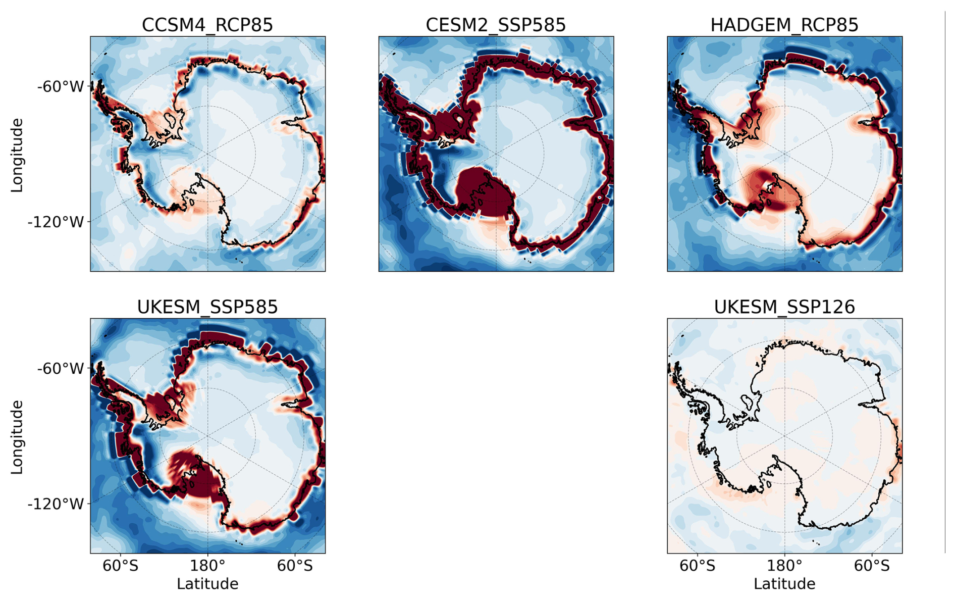
Figure 2 Surface mass balance (SMB) anomalies simulated by the five ESMs. The last year of the original datasets, which is 2300 for all simulations except the NorESM simulations, which end in 2100 is shown. Anomalies are added directly to the modelled present-day SMB from RACMO (Van Wessem et al., 2018) annually in the continuation simulations. The observed grounding line position is shown in black.

Four of the ESMs (CESM4, HadGEN2-ES, CESM2 and UKESM) were run forward from the historical period until 2300, with high emissions continuing long after 2100 in the high-emission scenarios (RCP85 and SSP5-8.5). For these models, we fix the thermal forcing and SMB anomalies at the 2300 values during the last 200 years of the simulation. NorESM, however, was run only until 2100. After 2100, the NorESM forcing in our simulations is held fixed at late 21st century values. Thus, the NorESM forcing is not directly comparable to the other ESMs after 2100.

3 Results

3.1 Initialization evaluation

Figures 3–5 present the key performance metrics for the equilibrium and transient initializations, namely the difference between observed and modelled ice thickness, surface ice velocities and mass change rates. Figures S4 and S5 in the Supplement show the spatial patterns of the ice thickness and surface velocity errors with respect to observations, and the optimized quantities for both initializations.

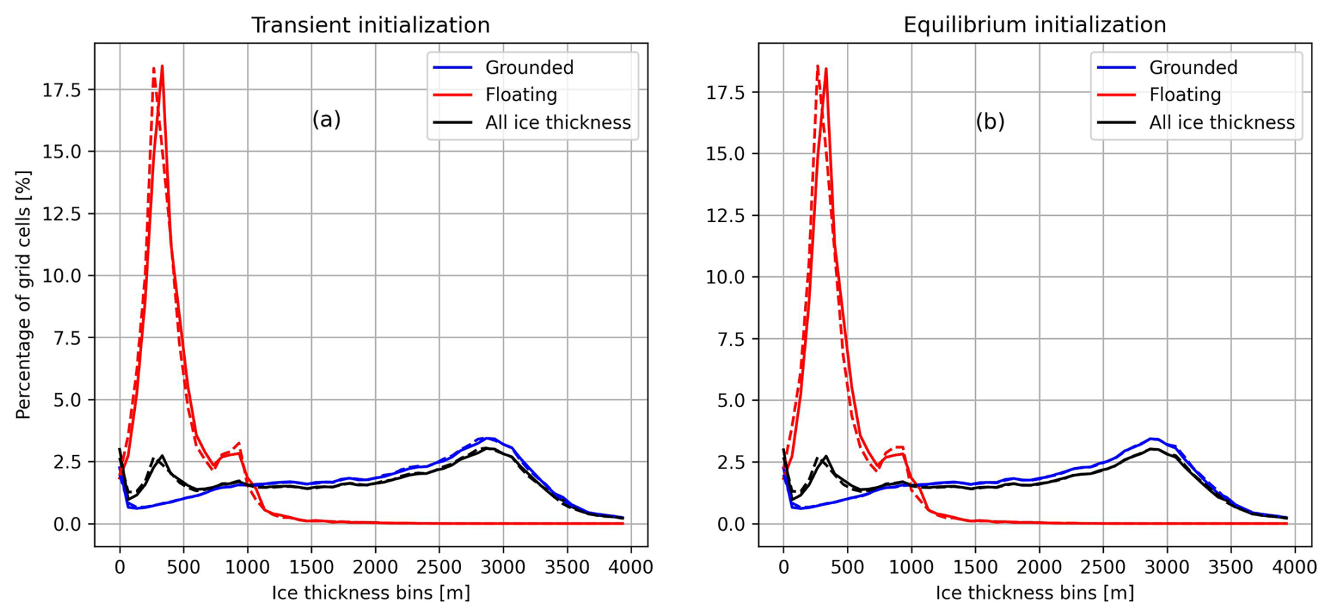
Figure 3 Binned ice thickness (m) for the observed (solid) and modelled ice (dashed lines). The present-day condition of the transient initialization is shown on the left, the equilibrium simulation on the right. For the transient initialization, the root mean square errors (RMSEs) for floating ice, grounded ice and in total are respectively 44, 31 and 35 m. For the equilibrium initialization they are respectively 50, 23 and 30 m.

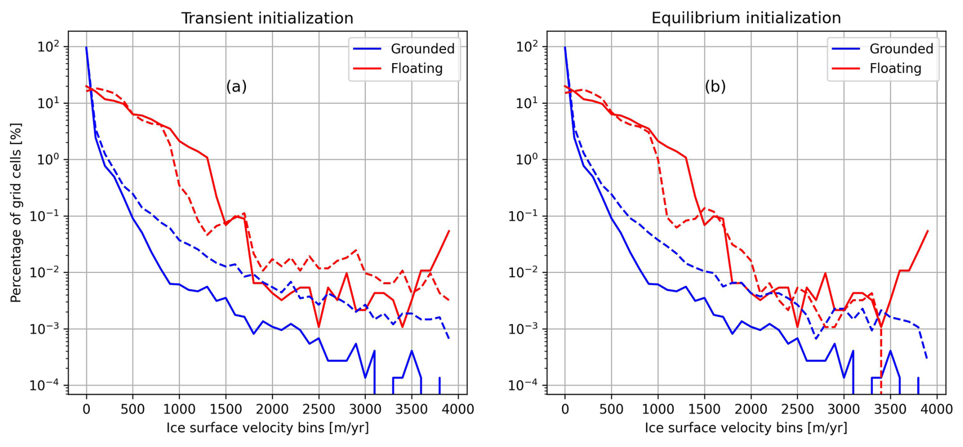
Figure 4 Binned ice surface velocities (m yr⁻¹) for the observed (solid) and modelled ice (dashed lines). The present-day condition of the transient initialization is shown on the left, the equilibrium simulation on the right. For the transient initialization, the Root Mean Square Errors (RMSEs) for floating ice, grounded ice and in total are respectively 201, 112 and 143 m yr⁻¹. For the equilibrium initialization they are respectively 202, 98 and 130 m yr⁻¹.

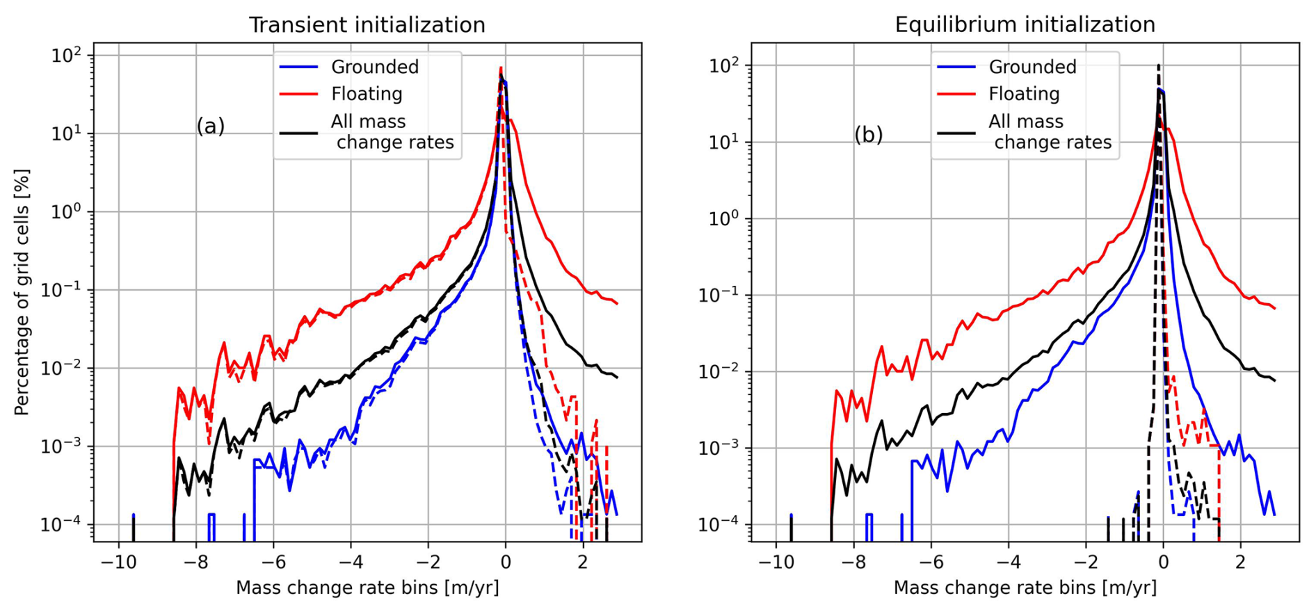
Figure 5 Binned mass change rates for the observed ice (solid lines) and the modelled ice (dashed lines). The transient initialization is shown on the left, and the equilibrium initialization on the right.

Overall ice thickness biases are low (Fig. 3), especially compared to the velocity errors. In both initializations, we tune towards an observed ice thickness target and not to an ice surface velocity target. The velocity biases are relatively high, but still of the same order of magnitude as many ISMIP6 models (see Seroussi et al., 2020). Including the present-day mass change rates increases the ice thickness and ice velocity RMSE slightly. Furthermore, in areas where large thinning rates are observed, such as PIG and TG, the dynamic imbalance pseudo-flux in Eq. (9) adds considerable mass during the spin-up, which brings the modelled ice fluxes across the grounding line in the transient initialization more in line with observations than in the equilibrium initialization, following Van Den Akker et al. (2025, 2026). Using the same flux gates and calculation as Van Den Akker et al. (2025), the observed ice fluxes in this study at PIG and TG are 31.1 and 26.1 km² yr⁻¹, respectively. In the equilibrium initialization, those fluxes are 17.0 and 17.4 km² yr⁻¹, hence much lower than observed. Using the present-day mass change rates and the initialization as described in Sect. 2 results in PIG and TG fluxes of 30.4 and 24.5 km² yr⁻¹, which are in good agreement with observations.

In areas with observed thickening in the dataset of Smith et al. (2020), such as at the EAIS, the magnitude of the sum of all ice fluxes (including the pseudo flux in Eq. 10) can become similar to or larger than the negative of the SMB. This requires for these locations, for an equilibrated transient ice sheet, a largely reduced ice flux divergence or even ice flux convergence compared to the equilibrated equilibrium ice sheet. Since ice velocities are low at these locations, and therefore the ice flux is small, the basal friction cannot always decrease the ice velocity enough to reach a steady state with the correct ice thickness, and hence the ice sheet thins locally until a new equilibrium is reached. Consequently, adding the observed present-day mass change rates in these locations yields a negative modelled ice thickness bias, visible on the EAIS in Fig. S2. This increases the RMSE of the modelled ice thickness with respect to observations.

The ice surface velocity biases are generally low in both initializations, except for the Siple coast glaciers and the Ronne ice shelf. For the Siple Coast, the thickness biases are low, indicating that the friction constant optimalization in these spots can nudge the modelled ice thickness close to observations, typically with a low C_c in the ice streams. This apparently leads to an overestimation of the ice surface velocity in these ice streams, which can be counteracted by locally tuning parameters related directly to the ice velocities, like the viscosity or the flow enhancement factor. However, the relative error in these ice streams, where the ice surface velocities exceed 2 km yr⁻¹, is still small.

The same holds for the Ronne shelf, where the modelled ice surface velocities are too low. The ice thickness error for the Filchner-Ronne shelf in both initializations is low, again indicating that the nudging of δT is capable in reproducing the observed ice thicknesses. However, the nudging of δT does not alter the modelled ice thickness by changing the ice velocities as it does for the friction constant optimalization. To obtain a better fit, just as with the glaciers at the Siple Coast, parameters directly related to the ice velocities can be nudged. This decreases the misfit between modelled and observed ice surface velocities as shown by Van Den Akker et al. (2026), but it also introduces another time-constant but spatially varying parameter with associated uncertainties and the risk of over-tuning.

Figure 5 shows the binned mass change rates from the observations and both model initializations. The transient initialization reproduces the observed thinning rates almost perfectly. For positive rates, the modeled values begin to diverge from the observations in grounded regions where observed thickening exceeds 0.5 m yr⁻¹, which occurs in less than 0.01 % of the modeled grid cells. This discrepancy arises because the model can no longer reduce ice flux by increasing friction; C_c in Eq. (4) has reached its upper limit of 1. The surface mass balance and ice inflow into the cell become insufficient to reproduce the observed mass change. These cases of underestimated ice sheet thickening occur mainly in the interior of the EAIS, a region with little to no dynamic connection to the WAIS.

For floating grid cells, the model cannot reproduce observed thickening rates because ice accretion is not formally represented in the ISMIP6 basal melt parameterization. This restriction arises from the inability to specify where the positive mass change terms Eq. (9) should be applied, on top or on the bottom of a floating ice column.

The equilibrium simulation presents a different pattern. As expected, it fails to capture the observed present-day mass change rates completely, as it was initialized to be in equilibrium. Consequently, it exhibits minimal model drift; only 0.001 % of the modeled grid cells show a drift greater than 0.1 m yr⁻¹.

3.2 Schematically forced Antarctic mass change

Figure 6 presents the integrated GMSL rise resulting from the schematic warming experiments, for both the ASE and the entire AIS. Starting from the transient initialization, applying a uniform and abrupt ocean warming to the ASE triggers an earlier onset of collapse with increasing temperatures, with diminishing sensitivity at higher ocean temperatures, but a larger rate of GMSL rise. The impact of ocean warming is larger in simulations initialized without present-day mass change rates. This can be attributed to the optimized parameter δT, which tends to be lower in these runs. As a result, adding 0.2 K of ocean warming leads to a relatively larger increase in effective ocean temperatures compared to simulations that include present-day mass change rates, where δT is typically higher.

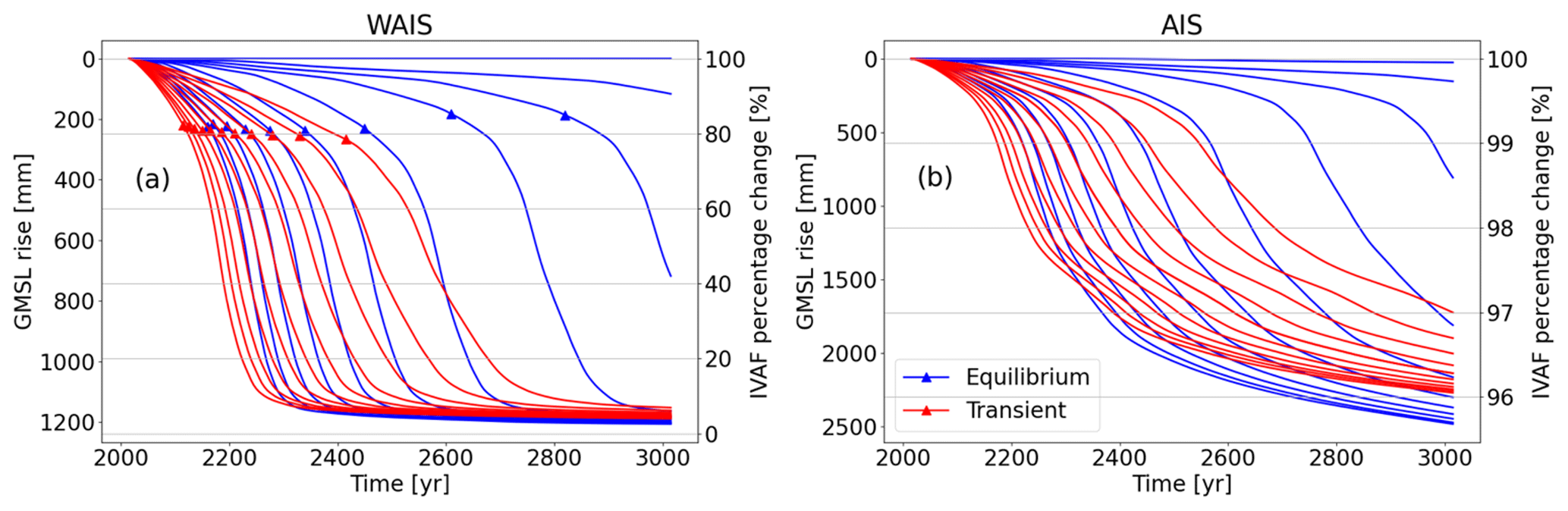
Figure 6 Ice Volume Above Floatation response to sudden, uniform ocean warming of the ASE sector, represented as GMSL rise (left y axis) and as percentage of what was originally present in the ASE region. (a) integrated mass loss in the ASE, where Thwaites Glacier and Pine Island Glacier are situated. Left y axis shows the GMSL rise in mm and the Ice Volume Above Floatation (IVAF) in percentage of the initial value. (b) The same for the whole AIS. Red lines indicate simulations starting with the observed mass change rates, blue lines indicate simulations starting from an equilibrium. From right to left (later collapse to earlier collapse) the simulations are forced with 0 to 2 K of ocean warming with steps of 0.2 K. Triangles indicate the timestep when the bedrock ridge approximately 50 km inland of the present-day TG grounding line ungrounds, depicted by the line AB in Fig. S6.

Interestingly, the equilibrium simulations (blue lines in Fig. 6) show a greater long-term GMSL contribution from the AIS compared to the transient simulations. The equilibrium runs are more sensitive to ocean warming, which can be partly attributed to a larger relative increase in δT, and to the stabilizing effect of including present-day mass change rates. Specifically, incorporating these rates makes the Kamb Ice Stream (see Fig. S6 in the Supplement) more stable, as it is currently thickening (Smith et al., 2020). A more stable Kamb ice stream acts as a brake on the retreat of Siple Coast glaciers once the ASE has lost its grounded ice. In this scenario, the retreat of the grounding line and subsequent ice sheet collapse are less able to propagate beyond the ASE, across the WAIS ice divide, and into the Siple Coast region. In contrast, in the equilibrium simulations, where this stabilizing effect is absent, such large-scale collapse can occur more easily.

To investigate the impact of different initial conditions, we subtracted the results of the no-perturbation simulations (i.e. 0 K of added ocean warming in the ASE) from their corresponding schematically forced simulations (Fig. 7). In the case of the equilibrium initialization, the no-perturbation experiment resulted in negligible mass loss, so the mass loss in the forced experiments due to the applied ocean forcing is almost the same as the difference between the forced scenarios and the no-perturbation experiment. In contrast, the unforced transient initialization exhibits a collapse of the WAIS, so Fig. 7 shows the deviation from this evolution due to the added ocean forcing.

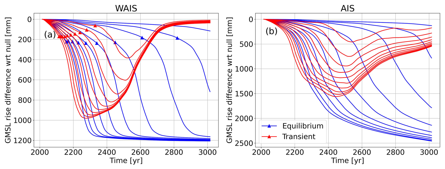
Figure 7 All schematic warming scenarios with the control experiment (i.e. 0 ocean warming) subtracted. For the ASE (a) and the AIS (b) in terms of GMSL rise. Triangles indicate the timestep when the ridge in the bedrock approximately 45 km inland of the present-day TG grounding line ungrounds, depicted by the line AB in Fig. S6. Red lines indicate simulations starting with the observed mass change rates; blue lines indicate simulations starting from an equilibrium. From right to left (later collapse to earlier collapse), the simulations are forced with 0.2 to 2 K of ocean warming with steps of 0.2 K. Triangles indicate the timesteps when the line AB in Fig. S6 ungrounds completely.

The simulations starting from the transient initialization have a much different response than those starting from the equilibrium initialization. For the first 250 (strong forcing) to 600 (weak forcing) years, the impact of ocean warming is larger for the transient initialisation simulations than for the equilibrium initialization simulations. Positive feedbacks drive the collapse of the WAIS, and these feedbacks are initiated earlier if the simulations start out-of-balance. After the collapse of TG and PIG, the impact of ocean warming ceases in the transient initialization simulations, as the GMSL rise contribution slows down in the final phase of the collapse (Fig. 6b) and the WAIS can only collapse once. This ceasing effect will not occur for the equilibrium initialization simulations, as the ocean forcing induces all the GSML rise contribution and the collapse of the WAIS, which otherwise would not happen.

In Fig. 8, increasing ocean warming is correlated with an earlier onset of TG collapse, which in our simulations consistently acts as the precursor to WAIS collapse. In this study, all collapse events initiate at TG. The onset of collapse is defined as the first timestep at which the bedrock ridge, 50 km upstream the current grounding line (see Fig. S6) becomes entirely free of grounded ice. The role of this bedrock ridge is discussed in more detail by Van Den Akker et al. (2025). The results show that higher ocean temperatures lead to earlier collapse, but with progressively smaller shifts in timing. This suggests the presence of a limit on the onset of collapse; TG cannot collapse before ∼2100 without more than 2° of ocean warming. Meanwhile, the maximum GMSL rise rate during the collapse increases linearly with ocean temperature, indicating that while earlier collapse timing shows diminishing returns, the rate of sea-level rise keeps on intensifying with stronger forcing. The additional sea-level contribution can come not only from PIG and TG, but also from the neighbouring Pope, Smith and Kohler glaciers, which are in the same basin as TG and therefore receive the same ocean warming. Furthermore, simulations starting from an ice sheet in equilibrium have the collapse delayed by multiple centuries compared to the transient initialization simulations. Here, however, warmer ocean waters still bring the collapse onset forward, without approaching a limit. It is noteworthy that the maximum GSML rise rate, if reached, is comparable to transient initialization runs.

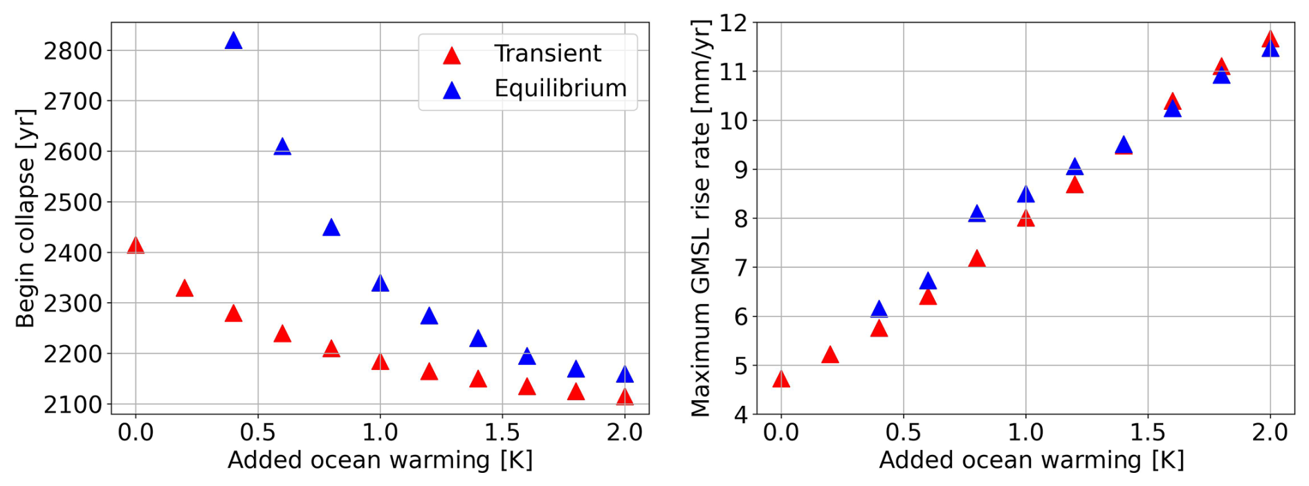
Figure 8 Impact of ocean warming on the beginning of the collapse and maximum GMSL rate. (left) The beginning of the WAIS collapse defined as the ungrounding of ridge AB in Van Den Akker et al. (2025) as function of added uniform and sudden ocean warming in the ASE. Blue dots represent simulations. (right) The maximum GMSL rise rate modelled in the same simulations, also as function of the added ocean warming.

3.3 Realistically forced future Antarctic mass change

Figure 9 shows the simulated integrated ice sheet mass loss in the Amundsen Sea Embayment (ASE) as well as for the entire Antarctic Ice Sheet. Until 2150, the projected mass loss is largely determined by the initialisation method; hence the current dynamic imbalance sets the short term mass loss of the ASE. After 2150, all simulations project eventual WAIS collapse, in most cases before 2500. Simulations initialized with the transient initialization configuration (solid lines) predict faster ice mass loss and an earlier collapse than those initialized with the equilibrium initialization configuration (dashed lines). This accelerated ice mass loss when using the transient initialization compared to the equilibrium initialization and collapse due to transient initialization occurs 50 to 100 years earlier under low emission scenarios (SSP126 or RCP26) and 25 to 50 years earlier under high-emission scenarios. These findings highlight the impact of the present-day imbalance on WAIS projections and emphasize the need to include those in regional simulations. The influence of this imbalance is more pronounced under cooler scenarios, where future ocean warming and surface melting is less dominant. In warmer scenarios (RCP8.5 and SSP5-85), the strong ocean forcing and net negative SMB diminish the relative impact of model initialization choices. Similar results have been described for glacial isostatic adjustment applications by Van Calcar et al. (2024) who argue that the details of the GIA matter relatively more for small forcing and relatively less for strong forcing.

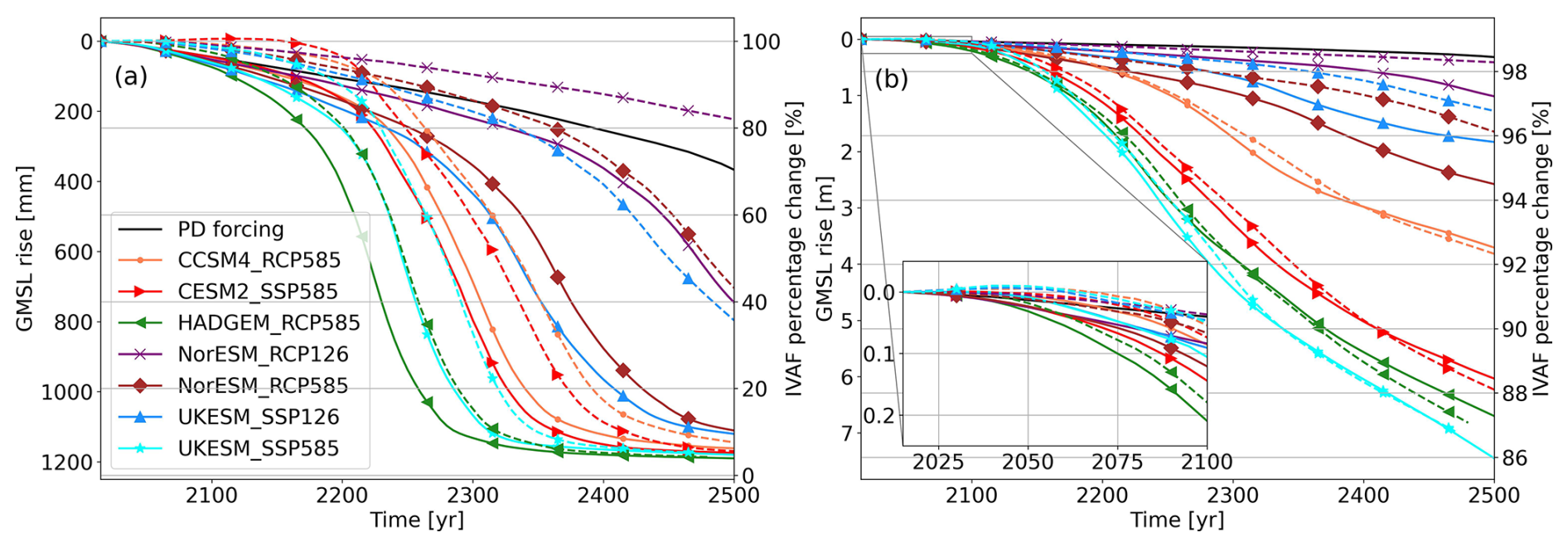
Figure 9 Integrated mass loss in the ASE, where Thwaites Glacier and Pine Island Glacier are situated (a). Left y axis shows the GMSL rise in mm and right y axis the Ice Volume Above Floatation in percentage of the initial value. The same for the whole AIS (b). Solid lines indicate simulations starting with the observed mass change rates, dashed lines indicate simulations starting from an equilibrium. Colors indicate the ocean forcing scenario used. The black line indicates an unforced transient initialization simulation. PD-forcing denotes a simulation without any additional ESM forcing, similar to what was done by Van Den Akker et al. (2025).

For the whole AIS and in the perspective of modelled multi-metre GMSL rise contribution, the present-day imbalance has an impact on the AIS mass loss before 2100. All simulations starting from the transient initializations show more integrated mass loss over the AIS in 2100 compared to the simulations starting from the equilibrium initialization, with in most cases a doubled GMSL rise contribution when using the present-day observed mass change rates, except for the simulations forced by HADGEM_RCP585 when considering the ASE region. This forcing contains early ocean warming and little increases in the SMB in the beginning of the simulation, overshadowing almost immediately the differences caused by the transient and equilibrium initialization with a much larger signal. However, simulations forced by both UKESM forcing datasets show the largest and fastest increase in sea level rise over the whole AIS.

After 2150, the emission scenario has the largest impact on the projected mass loss. For the high-end and low-end scenarios, the projected GMSL rise is 1–6 and 1–2 m, respectively. The difference in projected ocean changes by various ESMs is the next largest source of uncertainty; this will be discussed more below. Lastly, the effect of equilibrium or transient initialisations on the projected GMSL rise from the entire AIS is, in a relative sense, much smaller than in regional simulations focussing on the ASE, or on short-term projections of the AIS. In 2500 for the whole AIS, the difference between transient and equilibrium starting runs is about 1 %–2 % IVAF change. At a regional ASE simulation and before 2500, the difference can be up to 10 %–20 % IVAF, a tenfold difference.

For high-emission scenarios, incorporating the mass change rates even decreases the GMSL rise contribution. This can be explained by the strength of the warming in these scenarios, which leads to the collapse of major ice shelves in both transient and equilibrium initialized simulations. At the same time, observed thickening in parts of the grounded East Antarctic Ice Sheet (EAIS) continues in the future simulations, offsetting some of the mass loss from West Antarctica. As a result, mass loss in the WAIS is partially balanced by the increase in thickness in Dronning Maud Land, yielding a similar projected GMSL rise contribution, see Fig. 9. We argue that the spatial distribution of mass change in the transient initialization simulations is more physically justified compared to the pattern of mass loss in the equilibrium initialization cases, since the former captures a projected thickening of the EAIS until 2100, in line with recent studies on the forced future of the modelled Antarctic Ice Sheet (Siahaan et al., 2022; Coulon et al., 2024; Klose et al., 2024; O'Neill et al., 2025) and in line with present-day observations (Smith et al., 2020).

The simulations forced with NorESM output (RCP126 and RCP585) show much less mass loss than the others, as both NorESM simulations have less warming and more enhanced accumulation than the other ESM runs. The NorESM output assumes a constant climate after 2100, while output from the other ESMs assumes ongoing warming through 2300.

Next, we discuss the modelled patterns of ice shelf and grounding line retreat. Figure 10 shows the number of simulations containing ice (Fig. 10a) and grounded ice (Fig. 10b) across Antarctica for the year 2500. The most significant reduction in grounded ice area occurs in the WAIS. Aside from Wilkes Land, the grounding line retreat is limited in the EAIS as for most of the coastline, the inland bedrock is close to or above sea level. All simulations predict substantial grounded ice loss in Thwaites Glacier, as already clear from Fig. 6a. While not all scenarios result in a full WAIS collapse, several high-emission scenarios show complete loss of floating ice at the current locations of PIG and TG.

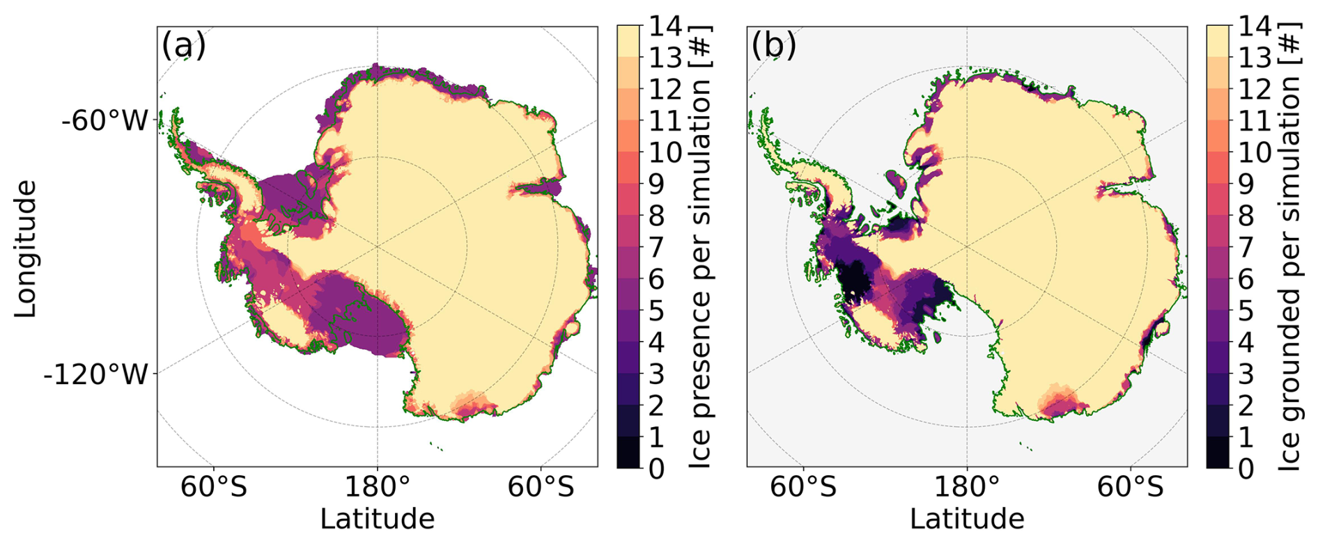
Figure 10 Ice present (a) and grounded (b) at the end (2500) of every simulation per grid cell, summed over all 14 simulations: with 7 ESM scenarios and the transient and equilibrium initialization.

For half the simulations, the Filchner–Ronne shelf and the Bungenstock Ice Rise (near the southern margin of the Ronne ice shelf) have respectively disappeared and completely ungrounded by 2500. More than half (9 out of 14) simulations end with the Ross shelf completely melted, in some cases along with glaciers at the Siple coast. As our simulations do not model calving for retreated ice shelves, this disintegration is entirely due to enhanced basal melting by warmer ocean waters. In fact, in simulations where the Filchner-Ronne or the Ross shelves effectively disintegrate, the Bungenstock Ice Rise or the Siple Coast also deglaciate, showing a direct relation between the large floating ice shelves and their upstream tributary glaciers.

This clear connection between floating and grounded ice mass is further assessed in Fig. 11. The floating ice mass and percent change of IVAF since 2015 are shown per region (Filchner-Ronne, Ross and ASE as delineated in Fig. S3) in this figure. Both the Filchner-Ronne and Ross shelves display similar trends. Some ESM forcings result in little change in modelled floating ice mass on the shelves during the simulation. For the Ross shelf, this occurs under UKESM-SSP126 and NorESM_RCP26, while for Filchner-Ronne the same applies with the addition of NorESM_RCP85. In all other scenarios except NorESM_RCP85 for Ross, the volume of floating ice diminishes. This pattern is irrespective of the transient or equilibrium initialization: the dashed and solid lines in Fig. 11 show little difference. These regions are currently relatively stable compared to the ASE (Smith et al., 2020). As a result, incorporating the small observed mass change rates in those regions does not affect the mass loss in future projections.

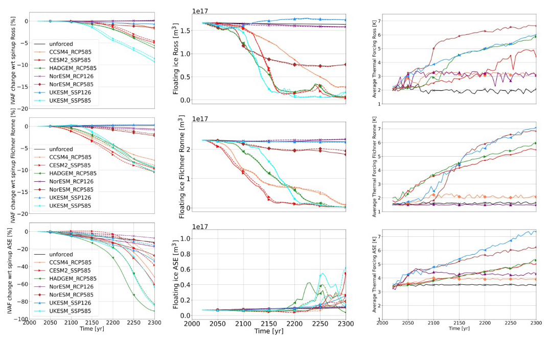
Figure 11 Ice volume above floatation (IVAF), floating ice mass and average thermal forcing for Ross (upper row), Filchner Ronne (middle row) and ASE (bottom row) per basin until 2300. The left column shows the IVAF as a percentage of what was present at the initialization; the middle column shows the total mass of floating ice per region; the right column show the average thermal forcing at 510 m below sea level at the calving front.

The loss of floating ice mass is closely tied to the average thermal forcing in each region, as shown in Fig. 11. For the Filchner-Ronne shelf, the percent change in IVAF, the floating ice mass loss and the average thermal forcing all follow a consistent pattern. Some ESMs simulate increased thermal forcing at the F–R calving front, which leads to near-complete shelf collapse and substantial ice mass loss. Others maintain thermal forcing near present-day levels, resulting in a largely intact ice shelf and minimal mass loss. A similar pattern is observed for the Ross shelf, the middle column in Fig. 11. The notable exception is NorESM_RCP85, which leads to a reduced Ross shelf in 2300 but not to a complete loss. In this simulation, thermal forcing rises sharply between 2050 and 2100 before stabilizing, which results from repeated climate forcing applied to the NorESM simulations. The early spike is enough to halve the shelf volume quickly, and the subsequent stabilization allows the remaining half to persist.

The ASE region exhibits a distinct pattern. At the beginning of each simulation, there is little floating ice present in the PIG and TG basins. The present-day shelves are small compared to F–R and Ross. As soon as the grounding line starts to retreat and the grounding line flux increases, a large shelf forms. However, if the thermal forcing is strong enough, this newly formed shelf rapidly melts, producing the increasing and then decreasing pattern of floating ice mass loss in the bottom row of Fig. 11. Van Den Akker et al. (2026) provide a more detailed discussion of the role of the shelves on the future dynamics of TG.

The loss of grounded ice mass and the reduction in floating ice volume are similarly related for the Ross and Filchner-Ronne basins. Once a critical fraction of floating ice is lost, the buttressing declines, leading to accelerated upstream flow of grounded ice, contributing to GMSL rise. To estimate this time lag between the onset of floating ice mass reduction and grounded ice loss, we calculated the time delay between 10 % floating ice mass loss of an ice shelf sector and 5 % grounded ice mass loss from that sector for each simulation and for the Filchner-Ronne and Ross sectors. We excluded the ASE from this analysis as in this region buttressing has currently little impact on the ice dynamics (Favier et al., 2014; Robel et al., 2019; Lipscomb et al., 2021; Gudmundsson et al., 2023; Van Den Akker et al., 2025). Typically, the delay between losing 10 % of floating ice and losing 5 % of grounded ice is on the order of decades (Table 1). In general, glaciers feeding into the Filchner-Ronne ice shelf respond slightly more rapidly than those along the Siple Coast, indicating that the Filchner-Ronne shelf provides more buttressing. Therefore, once 10 % of the Filchner-Ronne's floating ice volume is lost compared to present-day levels, most simulations show that 5 % of grounded ice mass loss (58.7 cm GMSL rise) will follow.

Table 1 Delay in years between a floating ice mass loss of 10 % and an IVAF loss of 5 % (5 % translates to 58.7 cm GMSL rise from FRIS and 24.4 cm from Ross). The symbol “×” denotes simulations in which the 10 % ice volume above floatation threshold and/or the 100 mm SLR contribution is never reached. The Filchner-Ronne shelf is abbreviated with “FRIS”, the Ross shelf with “Ross”.

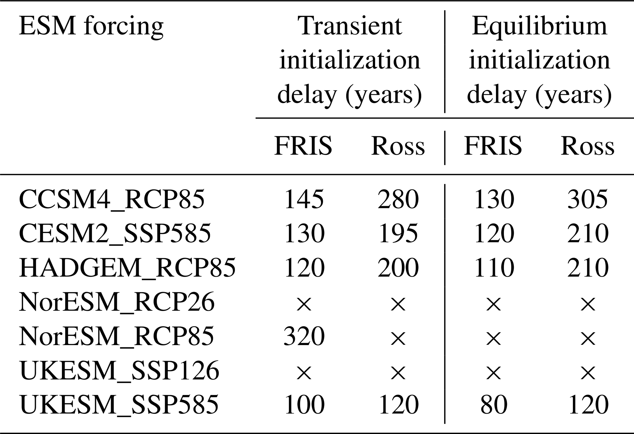
Except for NorESM_RCP85, the delay in deglaciation of the FRIS is higher when doing a transient initialization compared to simulations starting from the equilibrium simulation, while the delay for Ross is often shorter. This is due to an opposite pattern in the mass change rates of Smith et al. (2020). The Filchner-Ronne shelf is currently thinning, but the grounded ice upstream is slowly thickening. This is reversed at the Siple Coast and the Ross ice shelf: here the shelf is thickening and the grounded ice mainly thinning. Adding the mass change rates as was done for the transient initialization makes the grounded ice upstream of the Filchner-Ronne shelf slightly more stable and at the Siple Coast slightly less stable, and therefore slightly more sensitive to floating ice mass loss.

Significant floating ice volume loss leads in most cases within a century to significant grounded ice loss and sea level rise. This can be explained by two mechanisms: the sensitivity of the basal melt parameterization to changes in the ocean temperatures (e.g. the sum of TF_base and δT in Eq. 6) and the location of large SMB anomalies. Regarding the former, when deriving Eq. (6) with respect to the sum of TF_base and δT and filling in parameter values, we find that the basal melt parameterization has a temperature change sensitivity of ∼11 $\mathrm{m}{\mathrm{yr}}^{-\mathrm{1}}{\mathrm{K}}^{-\mathrm{1}}$ when the sum of TF_base and δT is 1 K, increasing linearly (e.g., when the sum is 2 K, the melt sensitivity is 22 $\mathrm{m}{\mathrm{yr}}^{-\mathrm{1}}{\mathrm{K}}^{-\mathrm{1}}$). For some scenarios, the ocean forcing applied can be several degrees K, causing an increase in basal melt of hundreds of metres per year, while the SMB anomalies range only from −2 to 2 m yr⁻¹.

Finally, in Fig. 12, we investigate whether the present-day imbalance adds linearly to future climate forcing, by subtracting the no-forcing experiment from all forced experiments. Compared to Fig. 7, the differences between the transient and equilibrium simulations are much less pronounced, hence the long-term impact of the current imbalance and future warming looks to add largely linearly. Only when the transiently initialized simulation is in the collapse phase of TG and PIG, the ESM forcing causes a non-linear enhancement of the GMSL rise contribution from the ASE sector (Fig. 12a). This is caused by enhanced ocean warming in the ASE sector compared to the initializations, which is most pronounced in the HADGEM_RCP85 scenarios. The other simulations shown in Fig. 12 that show a distinct difference in response between the equilibrium and transient simulations are UKESM_SSP585 and CESM2_SSP585, both of which include severe drops in the surface mass balance over the grounding line are of the ASE sector (see Fig. 2). All other ESM forcing datasets contain a smaller difference in ocean temperature with the spin-up (see Fig. 1), as well as smaller SMB anomalies, and therefore show a less pronounced difference with their respective control scenario.

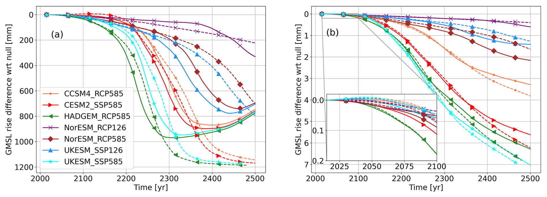
Figure 12 Induced mass loss by the ESM forcings with respect to the unforced simulations, for (a) the ASE and (b) the AIS in terms of GMSL rise. Solid lines indicate simulations starting with transient initialisation, dashed lines indicate simulations starting from the equilibrium initialization. Colors indicate the ocean forcing scenario used.

Prior to the collapse phase, the simulations align much more closely than in Fig. 7. This may be explained by the fact that, as the TG and PIG basins approach collapse, their mass loss becomes increasingly governed by ice dynamics and less by external forcings. Consequently, simulations starting from equilibrium conditions are more sensitive to gradual warming, which corresponds to the faster increase in GMSL contribution observed in the transiently initialized simulations (Fig. 11, bottom row). As in Fig. 7a, the influence of the ESM forcing ceases after the collapse, since WAIS also collapses in the transient simulation without forcing, and WAIS can only collapse once. Lastly, the difference between the transiently and equilibrium-initialized simulations is minimal for the AIS as a whole (Fig. 12b), as the substantial projected GMSL contribution by 2500 from AIS primarily originates from regions outside the ASE sector, which currently remain in balance (Fig. 11).

4 Discussion

In this study, we show that including the observed present-day mass change rates in an ice sheet model (CISM) improves the quality of projected ice mass loss for the coming century (up until 2100), because it is consistent with the currently observed GMSL rise contribution. Before 2100, including the present-day mass change rates leads to considerably higher GMSL rise contributions from the AIS, regardless of the ESM forcing chosen. After 2100, dynamic effects like a TG and PIG collapse start to develop, leading to accelerating mass loss. Including the present-day mass change rates accelerates a modelled WAIS collapse by 25 to 100 years in forced simulations. In 2500 for the whole AIS, the difference between transient and equilibrium starting runs is about 1 %–2 % IVAF change. In regional ASE simulations and before 2500, the difference can be up to 10 %–20 % IVAF, a tenfold difference.

At the start of our simulations we find a sea level rise rate of 0.1–0.5 mm yr⁻¹ when using the transient initialization method. This is in line with the observed rates reported by Cronin (2012), Smith et al. (2020) and Fox-Kemper et al. (2021). In 2100, our spread in projected sea level rise from the WAIS and AIS is about 5–25 mm, comparable to the present-day observed rate (approximately 0.3 mm yr⁻¹) and in line with Van De Wal et al. (2022). This range is similar to values reported by Edwards et al. (2021), Coulon et al. (2024), Klose et al. (2024), Seroussi et al. (2023), and O'Neill et al. (2025). In our ensemble, we do not find any cases where the AIS gains net mass during our simulated period, contrasting with the results of Siahaan et al. (2022). They found increased snowfall to dominate over increased basal melting, which leads to a net mass gain until 2100, with higher mass gains with warmer climates. However, in simulations done with low climate forcing, they found a steady decrease of ice mass at the WAIS, similar to the results presented in this study. When continued, this could in their simulation lead to the Marine Ice Sheet Instability and further enhanced mass loss beyond 2100, possibly outpacing mass gain through increased snowfall.

In 2300, our modelled ensemble shows a GMSL rise contribution of roughly 100–1200 mm from the ASE and 100–4500 mm for the entire Antarctic ice sheet. This large range is linked to dynamic instabilities caused by ice sheet thinning earlier in the simulation. Our ensemble almost captures the range reported by Seroussi et al. (2024), Greve et al. (2023) and Payne et al. (2021), with the exception of the cases where the AIS is growing (i.e., when a negative GMSL rise contribution is simulated). The dynamic instability leading to the WAIS collapse is featured in all our simulations, causing large mass losses and thereby compensating any (small) mass gains on the EAIS. Furthermore, the ESM forcing used shows predominantly warming ocean waters and a decreasing SMB over the whole AIS from present-day until 2300 with time, in contrast to Siahaan et al. (2022), in whose simulations to 2100 the SMB increase dominates over ice dynamical processes.

Our schematic experiments show that simulations initialized with present-day mass change rates respond less strongly to uniform ocean warming than those using equilibrium initializations. As expected, greater ocean warming triggers an earlier collapse of TG and, subsequently, the ASE basin but with diminishing returns: the most significant impact of additional warming is seen in the low-warming scenarios. Notably, the onset of collapse does not occur before 2100, even with 2° of ocean warming. This is in agreement with earlier WAIS collapse studies; Joughin et al. (2014) mention from 2200 onward, Robel et al. (2019) and Van Den Akker et al. (2025) mention approximately 500 years onward. This suggests a potential ice dynamical threshold that delays the TG collapse. However, the peak rate of GMSL rise during the collapse continues to increase linearly with additional ocean warming. This aligns with the contrasting patterns in Figs. 7 and 12: while the nonlinear enhancement of mass loss by additional ocean warming and present-day mass losses prior to the collapse of the ASE sector is very apparent in the idealized simulations, it is largely absent in the simulations forced with ESM data. Hence, we find that including the present-day mass loss rates increases the modelled GSML from the AIS mainly in the short term when mass loss is dominated by the ASE.

The relative unimportance of the SMB changes is related to the location of their anomalies. The largest anomalies are found near the coast of the AIS, where in many locations floating ice, or as the simulations progress, no ice at all exists. Therefore, the increased/decreased SMB is not contributing significantly to changes in projected GMSL rise from simulations forced by output from different ESMs. However, the SMB in the CMIP5 and CMIP6 models is determined using the present-day geometry of the Antarctic Ice Sheet. In our simulations, the ice sheet geometry changes drastically, with surface heights decreasing for most of the WAIS. Lower surfaces, through the lapse rate, will yield higher air temperatures and a more negative SMB, which could enhance mass loss more when this effect is incorporated. Ideally, ice sheet modellers should use coupled simulations where atmospheric models directly resolve the SMB of ice sheets based on their evolving geometries. This is computationally expensive and only done for the AIS in recent UKESM studies, such as Siahaan et al. (2022). Alternatively, simple parameterizations of this effect could be used (e.g. Fortuin and Oerlemans, 1990). A solution could be to use SMB emulators, but these have yet to be developed.

In many simulations shown in our study, all floating ice disappears from the Filchner-Ronne and Ross shelves. This is not uncommon in forced AIS simulations (Coulon et al., 2024; Seroussi et al., 2023; Seroussi et al., 2024). However, the disappearance of the big ice shelves is controlled by the amount of warming available in their cavities. CISM does not contain a submodule to simulate the overturning circulation in the ice shelf cavities, and neither did the ESMs from which the forcing was used in this study. The thermal forcing was only available in the open ocean bounded by the (observed) calving front of the AIS, and had to be extrapolated into the cavities. Therefore, it cannot be ruled out that the warming simulated in the cavities that lead to dramatic floating ice loss of the large ice shelves is caused (at least in part) by the extrapolation scheme. In essence, the extrapolation scheme now determines when the ice shelf cavities shift from a cold state, which they in are at present, to a warm state. Future studies could improve this aspect by using cavity-resolving ocean models (Scott et al., 2023), or an intermediate complexity 2D layer resolving model like LADDIE (Lambert et al., 2023).

We employed seven forcing datasets derived from five ESMs. Although forcing data were available only to the year 2300, our simulations extended to 2500. To enable CISM to run through 2500, we held the forcing fields (from 2300) constant over the years 2300–2500. This approach could introduce biases if conditions in 2300 differ substantially from those in the surrounding decades. To assess this, we compared the 20 year mean (2280–2300) thermal forcing and surface mass balance (SMB) anomalies, shown in Figs. S9 and S10 in the Supplement, with the values used for the year 2300 (Figs. 1 and 2). For ocean thermal forcing, the year-2300 fields closely match the 20 year mean across all datasets. SMB anomalies show minor differences between the year 2300 and the average of 2280–2300, most notably in the NorESM_RCP26 dataset over the Weddell Sea, but overall, the spatial patterns and magnitudes remain highly similar. These comparisons suggest that substituting the 20 year mean for the single year 2300 would not affect our results significantly.

We applied a no-advance calving approach: the calving front was restricted from advancing beyond its present-day observed position. While it was allowed to retreat, primarily due to significant increases in basal melt rates observed in most simulations, calving ceased entirely once the front retreated upstream of its current position. Although this is a conservative and somewhat unphysical representation, it serves as a simplified framework. Incorporating a more physically grounded calving law, accounting for factors such as stress and strain rates, rather than relying solely on modelled ice thickness, could improve predictions of ice mass loss. Integrating such advanced calving schemes into CISM is an area of active research.

5 Conclusion

In this paper, we show ocean-forced Antarctic-wide simulations conducted with the Community Ice Sheet Model until 2500. We test a new feature of the model: initializing with the present-day observed mass change rates. Schematic ocean warming causes a faster onset of TG collapse with diminishing returns but linearly increasing GMSL rise rates with additional warming. We furthermore find that including the present-day imbalance is important for regional WAIS simulations, where including the present-day mass change rates in a simulation speeds up Thwaites Glacier and Pine Island Glacier collapse by 25–100 years. Including the mass change rates doubles the AIS GMSL contribution in 2100 in our ensemble. For long-term continental AIS simulations beyond 2100, the choice of the ESM used is more important than the choice to include or not the present-day mass change rates in a century-timescale simulation. We find for all simulations that the AIS will continue to lose mass over the next five centuries, with uncertainties increasing strongly over time.

Our study highlights that, for simulations until 2500, the main ice losses happen in the Ross and Filchner-Ronne, preceded by mass loss in the ASE region, but the pattern is highly dependent on the extrapolation scheme of ocean properties into the ice shelf cavities. The mass balance of the floating ice shelves proves to be crucial for the grounded ice loss rate. Our simulations do not use a physically based calving scheme or a sub-shelf cavity-resolving ocean model. Replacing both processes with physically based parameterizations or sub-models will likely change the mass balance of the floating shelves and ultimately increase our confidence in sea level rise projections from the Antarctic Ice Sheet. Including a more physically based rather than a location-based calving flux will probably increase the modelled future mass loss of the AIS, and therefore project faster ice sheet retreat and as a consequence, more GMSL rise.