Competing processes determine the long-term impact of basal friction parameterizations for Antarctic mass loss

Previous studies do not agree on the magnitude of the influence of basal friction laws in sea-level projections. We use the Community Ice Sheet Model (CISM) to show that the sensitivity of the projected sea level rise to the choice of basal friction law depends on the specific geometric setting and the initial state of the ice sheet model. We find a geometry-driven connection between buttressing and basal sliding in the Amundsen Sea Embayment when performing multi-century future simulations based on the present-day observed imbalance of the Antarctic Ice Sheet, in which Thwaites and Pine Island glaciers eventually collapse. We perform two initializations which differ in their value of a free parameter that governs the effective pressure of ice grounded on bedrock below sea level. Both initializations lead to a modelled Antarctic Ice Sheet that well resembles present-day conditions (ice thickness, ice surface velocities and mass changes rates). Following each initialization, we run the model forward with present-day climate forcing. In one simulation, Thwaites Glacier collapses first, and in the other, Pine Island Glacier collapses first. When Thwaites Glacier collapses first, it creates a grounding line flux large enough to sustain an ice shelf that provides buttressing which largely balances the basal friction differences when using different basal friction parameterizations. A collapsing Pine Island Glacier, however, is sensitive to the choice of basal friction law. Thus, the regional evolution and its sensitivity to friction laws depend on initialization choices that are poorly constrained by observations. In both simulations, present-day ocean thermal forcing, which is a product of the inversion using the present-day imbalance, is sufficient to drive Thwaites and Pine Island collapse, but small differences introduce an uncertainty of about 500 years in the collapse timing.

1 Introduction

The projected Antarctic contribution to global mean sea level (GMSL) rise ranges from 0.03–0.27 m (SSP1.9) to 0.03–0.34 m (SSP8.5) in 2100 (Fox-Kemper et al., 2021). After 2100, uncertainty increases because of dynamical processes, leading to a possible multi-meter GMSL rise by 2300 (Fox-Kemper et al., 2021; Payne et al., 2021; Seroussi et al., 2024). By and after 2300, self-sustaining processes could cause the deglaciation of large parts of the West Antarctic Ice Sheet (WAIS) (Joughin et al., 2014; Cornford et al., 2015; Seroussi et al., 2017; Coulon et al., 2024; van den Akker et al., 2025).

The largest dynamic mass changes are currently ongoing in the Amundsen Sea Embayment (ASE) (Smith et al., 2020). The possible deglaciation of the two largest glaciers in this region, Pine Island Glacier (PIG) and the Thwaites Glacier (TG), is one of the main sources of uncertainty in future ice sheet behavior (Cornford et al., 2015; Feldmann and Levermann, 2015; Arthern and Williams, 2017; Pattyn and Morlighem, 2020; Bett et al., 2024; Seroussi et al., 2024). The grounding line of both glaciers rests on a retrograde bed, making them susceptible to the Marine Ice Sheet Instability (MISI, see Schoof, 2007b). Some studies (Joughin et al., 2014; Favier et al., 2014) suggest that those glaciers are already undergoing MISI-like retreat. Recent studies suggested that present-day ocean temperatures could drive complete deglaciation of this area over several centuries, without additional warming (Reese et al., 2023; van den Akker et al., 2025).

Sources of modelled ice sheet uncertainty include the neglect of important physical processes and a suboptimal initial state (Aschwanden et al., 2021). Several studies have attributed uncertainty in sea level prediction from ice sheet models to the choice of the basal friction parameterization (Brondex et al., 2017; Bulthuis et al., 2019; Brondex et al., 2019; Sun et al., 2020; Wernecke et al., 2022; Barnes and Gudmundsson, 2022; Berdahl et al., 2023; Joughin et al., 2024). These parameterizations are relations between the basal ice velocity and friction at the ice-bedrock interface. Generally, the existing relations, or basal friction laws, can be separated into two types. For the first type, the friction depends on the basal velocity raised to some power. Using an exponent of 1 results in a linear relation, but exponents between 0 and 1 are more common (Weertman, 1957; Budd et al., 1979; Barnes and Gudmundsson, 2022; Das et al., 2023). These are referred to as “power law friction”, and were originally developed to represent basal sliding over hard bedrock. For the second type, friction becomes independent of velocity for fast-flowing ice; this is known as “Coulomb friction” (Schoof, 2005; Tsai et al., 2015; Joughin et al., 2019; Zoet and Iverson, 2020). Coulomb laws were originally developed to represent sliding over soft, deformable till. Both types of basal friction law contain free parameters that can be tuned to match observed quantities such as ice sheet surface velocities or thickness.

Another source of uncertainty is the potential of ice shelves to provide a buttressing force on the inland ice sheet (Dupont and Alley, 2005; Gudmundsson, 2013; Fürst et al., 2016; Haseloff and Sergienko, 2018; Reese et al., 2018a). A buttressed ice shelf can act as a plug against glacier acceleration. An accelerating glacier has an increasing grounding line flux, transporting more ice to the ice shelf. If the thicker shelf can persist, this will increase its buttressing capacity and oppose the initial acceleration of the inland ice. Choices related to basal friction will influence both the velocity profile and the modelled buttressing of the simulated ice sheet and ice shelves.

Most of the literature argues that power law friction will result in less modelled ice loss and sea level rise compared to Coulomb friction, both for idealized experiments (e.g., MISMIP-style experiments, see Asay-Davis et al., 2016) and for realistic simulations of the Antarctic Ice Sheet (AIS). However, authors do not agree whether the difference is substantial (Brondex et al., 2017; Sun et al., 2020; Brondex et al., 2019) or not (e.g., Barnes and Gudmundsson, 2022; Wernecke et al., 2022). Furthermore, basal friction parameterization tests in realistic settings such as the ASE or the entire AIS are often done with enormous (ABUMIP; Sun et al., 2020) or unrealistic perturbations (Barnes and Gudmundsson, 2022; Brondex et al., 2019). Fewer studies have addressed the importance of the friction law for WAIS collapse driven by less extreme, more realistic forcing.

Here we use the Community Ice Sheet Model (CISM) (Lipscomb et al., 2019; Lipscomb et al., 2021) to investigate the sensitivity of grounding line retreat and ice mass loss to the choice of basal friction laws for the West Antarctic Ice Sheet for sustained present-day forcing. Building on the work of Brondex et al. (2017), we extend our simulations for 2000 years into the future, to capture the importance of significant grounding line retreat. We use the observed mass change rates from Smith et al. (2020) to initialize the AIS with observed rates of regional mass loss, as in van den Akker et al. (2025): by including the mass change rates in the ice continuity equation during the initialization period. We perform two initializations. In both initializations we tune ocean temperature perturbations to obtain a match between modelled and observed ice shelf thickness, and we tune spatially distributed coefficients in the basal friction laws to nudge the modelled thickness of grounded ice toward observations. The initializations differ in their treatment of the effective pressure of grounded ice resting on bedrock below sea level. We then continue our simulations with four widely used friction laws. We present a specific case in which a reduction in basal friction, caused by adopting a different basal sliding law, is offset by a corresponding increase in buttressing. Whether this compensation occurs depends on the glacier's geometric evolution; some but not all geometries allow these compensating effects. Hence, the intitialization can determine whether or not the modelled ice sheet evolution is sensitive to the choice of basal friction law.

In Sect. 2 we describe the four basal friction laws and two ways of calculating the buttressing capacity, as well as the ice sheet model CISM. In Sect. 3 we show the specific geometric setting of TG, PIG and the ASE. Section 4 presents the results of our two initializations and continuation experiments, followed by a discussion in Sect. 5 and conclusions in Sect. 6.

2 Methods

2.1 Basal friction

We test four basal friction laws. First, we use a regularized Coulomb sliding law proposed by Zoet and Iverson (2020), hereafter referred to as the Zoet-Iverson (ZI) law:

$$\begin{array}{}\text{(1)}& {\mathit{\tau }}_{\mathrm{b},\mathrm{ZI}}=C_{\mathrm{c}}(x,y)N(x,y){\left({\displaystyle \frac{u_{\mathrm{b}}}{u_{\mathrm{b}}+u_{\mathrm{0}}}}\right)}^{\frac{\mathrm{1}}{m}},\end{array}$$

where τ_b,ZI is the basal friction, N is the effective pressure, C_c is a spatially varying unitless tuning parameter in the range [0,1] controlling the strength of the Coulomb sliding, u₀ is the yield velocity, and m an exponent with the common choice m=3. For a short description of variables and units, see Tables S1 and S2. The parameter C_c corresponds to the tan ϕ term of Zoet and Iverson (2020), Eq. (3), in which ϕ is the friction angle, a material property of the subglacial till. This parameter is used to nudge the modelled ice sheet toward the observed thickness as described in the next section.

In addition to the ZI law, we consider three more relations:

$$\begin{array}{}\text{(2)}& {\displaystyle }{\mathit{\tau }}_{\mathrm{b},\mathrm{Powerlaw}}=C_p(x,y)\cdot u_{\mathrm{b}}^{\frac{\mathrm{1}}{m}}\text{(3)}& {\displaystyle }{\mathit{\tau }}_{\mathrm{b},\mathrm{Schoof}}={\displaystyle \frac{C_p{C}_{\mathrm{c}}N}{{\left[C_p^m{u}_{\mathrm{b}}+{\left(C_{\mathrm{c}}N\right)}^{\mathrm{m}}\right]}^{\frac{\mathrm{1}}{m}}}}{u}_{\mathrm{b}}^{\frac{\mathrm{1}}{m}}\text{(4)}& {\displaystyle }{\mathit{\tau }}_{\mathrm{b},\mathrm{Pseudoplastic}}=C_{\mathrm{c}}N{\left({\displaystyle \frac{u_{\mathrm{b}}}{u_{\mathrm{0}}}}\right)}^{\frac{\mathrm{1}}{\mathrm{pp}}}\end{array}$$

In these equations, C_p is a spatially varying constant. Equation (2) is the classical power law for sliding (“power law” hereafter) from Weertman (1957). Note that we use for m the same value as in Eq. (1); it regulates the strength of the power law friction. Equation (3), often referred to as the “Schoof law” (Schoof, 2005), is a regularized Coulomb friction law suggested for the Marine Ice Sheet Model Intercomparison Project third phase (MISMIP+) experiments (Asay-Davis et al., 2016) and used in CISM in Lipscomb et al. (2021). It is argued in the literature that Eq. (3) is preferred over Eq. (2) because it yields physically realistic behavior of a retreating glacier (Brondex et al., 2017; Brondex et al., 2019). Equation (4) is referred to as a “pseudoplastic” law, developed and used by Winkelmann et al. (2011); Aschwanden et al. (2016). It is also often referred to as a “Budd” law after Budd et al. (1979). This last sliding law is similar in behavior to the power law but includes the effective pressure N, as in Eq. (3), and a value for pp between 1 and 5.

The effective pressure N at the ice–bed interface is the difference between the ice overburden pressure and the subglacial water pressure. In our simulations, the effective pressure is lowered near grounding lines to represent the connection of the subglacial hydrological system to the ocean (Leguy et al., 2014):

$$\begin{array}{}\text{(5)}& N={\mathit{\rho }}_{\mathrm{i}}gH{\left(\mathrm{1}-{\displaystyle \frac{H_{\mathrm{f}}}{H}}\right)}^p\end{array}$$

where the flotation thickness H_f is given by

$$\begin{array}{}\text{(6)}& H_{\mathrm{f}}=max\left(\mathrm{0},-{\displaystyle \frac{{\mathit{\rho }}_{\mathrm{w}}}{{\mathit{\rho }}_{\mathrm{i}}}}b\right),\end{array}$$

and where ρ_i is the density of glacial ice, ρ_w is the sea water density, g the gravitational acceleration, H the ice thickness, b the bedrock height, and p a constant in the range [0,1]. When p=0, the effective pressure is equal to the ice overburden pressure ρ_igH. For values of p greater than zero and up to 1, the effective pressure is reduced in proportion to how close the ice column is to flotation. Where the flotation criterion is nearly satisfied (i.e., H_f≈H), choosing p>0 produces an effective pressure much lower than the full ice overburden. This can be seen as a first-order approximation of the hydrological conditions near grounding lines, where the parameterization in Eq. (5) has the strongest effect. This formulation of N provides a smooth transition in basal friction, bridging the finite value for grounded ice and the zero value for floating ice. Moreover, through Eq. (6) it links effective pressure to bedrock height, and it introduces a nonlinear dependence of effective pressure on ice thickness, whereas setting p=0 assumes a linear relationship. Note that the power law does not depend on the effective pressure. The four friction laws differ in their dependence on the ice basal velocities and are shown with typical values in Fig. 1. The power law and the pseudoplastic law differ clearly from the Schoof and ZI law as they do not approach a limit for high basal velocity. The Schoof and ZI law behave similarly, although the ZI law is slightly more sensitive to changes in velocity. The power law and pseudoplastic law show increasing basal friction with increasing velocity. This introduces a negative feedback: a decrease in friction initially increases velocity, which in the power law and pseudoplastic law will always increase the friction. In the other two laws, the basal friction asymptotes for high velocities to C_cN, which is pure Coulomb friction. This has the important implication that perturbations introduced to simulations using power law or pseudoplastic friction will be damped quicker and more locally. A sudden loss of buttressing leading to a local speedup of ice at the grounding line (where ice velocities often exceed 200 m yr⁻¹) will be “braked” more heavily by the power law, limiting the effect of the perturbation (far) upstream of the grounding line.

Three of the sliding laws depend on the effective pressure. This introduces a feedback between ice velocity and basal friction. If the basal friction decreases, the ice flux across the grounding line increases. This decreases the ice thickness upstream of the grounding line, further reducing N. Thinning grounded ice, for example caused by a loss of buttressing, can lower N and lead to thinning far upstream of the grounding line (Brondex et al., 2017, 2019).

Figure 1 The four friction laws with indicative values. Basal friction as function of the ice basal velocity for constant values of C_c=0.5, C_p=1000, N=1 000 000 Pa, u₀=250 m yr⁻¹, and m=3. Dashed lines are the same basal friction laws with N=500 000 Pa (black line). The power law is independent of N, so the solid and dashed red line are the same. Coulomb sliding asymptotes to the product C_cN for the dashed and solid lines.

2.2 Buttressing

We quantify the buttressing capacity of an ice shelf at the grounding line with two approaches. The first approach compares the stress balance at the grounding line to the stress boundary condition at the calving front. This buttressing number, defined as the ratio between the latter two stresses, has been used in several studies (Gudmundsson, 2013; Gudmundsson et al., 2023; Fürst et al., 2016) and as a parameter in the analytical grounding line flux of Schoof (2007a) and Schoof (2007b). Reese et al. (2018a) describe three ways to calculate the buttressing number, of which we choose Eq. (11) in their paper and adapt it according to Eq. (S1) in the Supplement of Fürst et al. (2016):

$$\begin{array}{}\text{(7)}& \mathit{\chi }=\mathrm{1}-{\displaystyle \frac{{\mathit{n}}_{\mathrm{1}}.\mathbf{R}{\mathit{n}}_{\mathrm{1}}}{\mathrm{2}{R}_{\mathrm{f}}}}\end{array}$$

The vector n₁ is the vector perpendicular to the grounding line, in our regular rectangular grid best approximated by the direction of the ice flow. The stress boundary condition at the “would be” (i.e. if there would be no shelf and hence no buttressing) calving front R_f is given by

$$\begin{array}{}\text{(8)}& R_{\mathrm{f}}={\displaystyle \frac{{\mathit{\rho }}_{i}g}{\mathrm{4}}}(\mathrm{1}-{\displaystyle \frac{{\mathit{\rho }}_i}{{\mathit{\rho }}_w}})H.\end{array}$$

The parameter R_f therefore is the stress boundary condition if there were a calving front at that position. The resistive stress tensor R is given by

$$\begin{array}{}\text{(9)}& \mathbf{R}=\left(\begin{array}{ll}\mathrm{2}{\mathit{\tau }}_{xx}+{\mathit{\tau }}_{yy}& {\mathit{\tau }}_{xy}\\ {\mathit{\tau }}_{xy}& {\mathit{\tau }}_{xx}+\mathrm{2}{\mathit{\tau }}_{yy}\end{array}\right).\end{array}$$

The variable χ in Eq. (7) has a value of 0 for areas that are unbuttressed: then the buttressing force equals the driving stress if the ice sheet ended at that point with an ice cliff. Values above zero indicate buttressing. Values below zero point to a tensile regime where the ice shelf is pulling grounded ice over the grounding line. As shown by Reese et al. (2018a), the buttressing number from the linearized stress balance approach depends on the choice of n₁ and R, and assumes that the stress tensor at the grounding line is determined by the buttressing capacity of the downstream shelf only.

The second approach to quantify the buttressing is by performing so-called shelf-removal experiments (e.g. Antarctic BUttressing Model Intercomparison Project (ABUMIP), Sun et al. (2020). In these experiments, floating ice is instantly removed, and the effect on the grounded ice in terms of acceleration is used to measure the buttressing capacity of the removed shelves. We define the acceleration number, in analogy to the definition of the buttressing number, by

$$\begin{array}{}\text{(10)}& \mathit{\alpha }=\mathrm{1}-{\displaystyle \frac{u_{\mathrm{before}}}{u_{\mathrm{after}}}}\end{array}$$

in which u_before and u_after refer to the local depth-averaged ice velocity before and after removing the shelf. This method of quantifying the buttressing is the simplest way of assessing shelf strength but provides only a temporal snapshot and requires an additional ice sheet model timestep to be calculated.

Both methods shown in Eqs. (7) and (10) are tested on a theoretical case (the Ice1r experiment of MISMIP+, see Asay-Davis et al. (2016) and on the present-day state of the Antarctic Ice Sheet, before using them in the continuation simulations in this study. These results for the buttressing can be found in the Supplement, Figs. S1–S3.

2.3 The Community Ice Sheet Model

The Community Ice Sheet Model is a thermo-mechanical higher-order ice sheet model, which is part of the Community Earth System Model version 2 (CESM2, Danabasoglu et al. (2020). Earlier applications of CISM to the Antarctic Ice Sheet retreat can be found in Seroussi et al. (2020); Lipscomb et al. (2021); Berdahl et al. (2023); van den Akker et al. (2025). The variables and constants used in the text and equations below are listed in Tables S1 and S2. All simulations in this study are done on a 4 km grid.

We run CISM with a vertically integrated higher-order approximation to the momentum balance, the Depth Integrated Viscosity Approximation (DIVA) (Goldberg, 2011; Lipscomb et al., 2019; Robinson et al., 2022). The momentum balance in the x-direction (the y-direction is analogous) is defined as:

$$\begin{array}{}\text{(11)}& \begin{array}{rl}{\displaystyle \frac{\partial }{\partial x}}& \left(\mathrm{2}\stackrel{\mathrm{‾}}{\mathit{\eta }}H\left(\mathrm{2}{\displaystyle \frac{\partial \stackrel{\mathrm{‾}}{u}}{\partial x}}+{\displaystyle \frac{\partial \stackrel{\mathrm{‾}}{v}}{\partial y}}\right)\right)+{\displaystyle \frac{\partial }{\partial y}}\left(\stackrel{\mathrm{‾}}{\mathit{\eta }}H\left({\displaystyle \frac{\partial \stackrel{\mathrm{‾}}{u}}{\partial y}}+{\displaystyle \frac{\partial \stackrel{\mathrm{‾}}{v}}{\partial x}}\right)\right)\\ & -\mathit{\beta }{u}_{x,\mathrm{b}}={\mathit{\rho }}_{i}gH{\displaystyle \frac{\partial s}{\partial x}}\end{array}\end{array}$$

Barred variables are depth averaged. Basal friction, which is parameterized in the ways described in Sect. 2.1, appears as the product of β and the directional velocity in Eq. (11).

Since the spatially varying parameters C_c and C_p in Eqs. (1)–(4) are poorly constrained by theory and observations, we use it as a spatially variable tuning parameter. We tune C_c using a nudging method (Lipscomb et al., 2021; Pollard and DeConto, 2012):

$$\begin{array}{}\text{(12)}& {\displaystyle \frac{\mathrm{d}{C}_{\mathrm{c}}}{\mathrm{d}t}}=-C_{\mathrm{c}}\left[\left({\displaystyle \frac{H-H_{\mathrm{obs}}}{H_{\mathrm{0}}\mathit{\kappa }}}\right)+{\displaystyle \frac{\mathrm{2}}{H_{\mathrm{0}}}}{\displaystyle \frac{\mathrm{d}H}{\mathrm{d}t}}-{\displaystyle \frac{r}{\mathit{\kappa }}}\ln {\displaystyle \frac{C_{\mathrm{c}}}{C_r}}\right]\end{array}$$

Where κ is the relaxation timescale, and r a parameter controlling the strength of the relaxation term. A higher value for r will “pull” the inverted C_c towards C_r. In the end-member case, where r is infinite, C_c and C_r are equal. The relaxation target C_r is a 2D field based on elevation, with lower values at low elevation where soft marine sediments are likely more prevalent, loosely following Winkelmann et al. (2011). We chose targets of 0.1 for bedrock below −700 and 0.4 for 700 m a.s.l., with linearly interpolation in between, based on Aschwanden et al. (2013).

Basal melt rates are calculated using a local quadratic relation with a thermal forcing observational dataset (Jourdain et al., 2020):

$$\begin{array}{}\text{(13)}& b={\mathit{\gamma }}_{\mathrm{0}}{\left({\displaystyle \frac{{\mathit{\rho }}_{\mathrm{w}}{c}_{\mathrm{pw}}}{{\mathit{\rho }}_{\mathrm{i}}{L}_{\mathrm{f}}}}\right)}^{\mathrm{2}}{\left(max\left[{\mathrm{TF}}_{\mathrm{base}}+\mathit{\delta }T,\mathrm{0}\right]\right)}^{\mathrm{2}}\end{array}$$

where TF_base is the ocean thermal forcing (the difference between the ocean temperature the local melting point) from Jourdain et al. (2020), interpolated to the modelled ice shelf base. The ocean temperatures are tuned in order for the floating ice to match the thickness observations of Morlighem et al. (2020), similar to Eq. (12) but with δT as tuning variable:

$$\begin{array}{}\text{(14)}& {\displaystyle \frac{\mathrm{d}\left(\mathit{\delta }T\right)}{\mathrm{d}t}}=-\mathit{\delta }T\left[\left({\displaystyle \frac{H-H_{\mathrm{obs}}}{H_{\mathrm{0}}\mathit{\kappa }}}\right)+{\displaystyle \frac{\mathrm{2}}{H_{\mathrm{0}}}}{\displaystyle \frac{\mathrm{d}H}{\mathrm{d}t}}\right]+{\displaystyle \frac{\left(T_{\mathrm{r}}-\mathit{\delta }T\right)}{\mathit{\kappa }}}\end{array}$$

As in Eq. (12), we add a term including a relaxation target T_r to penalize large deviations. In this case, the relaxation target is zero, since δT is a temperature correction to the dataset of Jourdain et al. (2020). The melt sensitivity γ₀ is chosen to be 3.0×10⁴ m yr⁻¹, which was used in Lipscomb et al. (2021) and van den Akker et al. (2025) to obtain basal melt rates in good agreement with observations and with a shelf-average δT close to zero in the Amundsen Sea Embayment.

The grounding line (GL) is not explicitly modeled in CISM, but its location can be diagnosed from the hydrostatic balance. Since we use a regular rectangular grid, the modeled GL cuts through cells. To prevent abrupt jumps in the basal friction and the basal melt rates close to the GL, we use a GL parameterization (Leguy et al., 2021), where we use a flotation function to weigh the basal friction and basal melt rates according to the percentage of a grid cell that is grounded.

2.4 Initializations

In this study, we use two initializations. The first initialization (labeled as “P05”) uses the observed ice thickness as a target, nudges free parameters in the basal friction (Eq. 12) and basal melt parameterizations (Eq. 14), and per construct starts a continuation run with the observed mass change rates from Smith et al. (2020). The second initialization, does the same but with a value of p=0.5 in Eq. (5). Both initializations are tested on their stability. We deem an initialization successful and `stable' when there is little to no instantaneous model drift once we turn off the inversions and keep our nudged parameters constant, and there are no significant changes in modelled ice sheet geometry when run forward for 2000 years, similar to what was done by van den Akker et al. (2025). These two initializations will serve as a starting point for continuation simulations done with the four different friction laws described above to produce a set of 8 forward simulations. We will rewrite free parameters in the friction laws to be able to start every forward simulations from a single initialization simulation.

2.4.1 P05 initialization (P05)

The P05 initialization uses Eqs. (12) and (14) to initialize an Antarctic ice sheet in equilibrium, with ice thicknesses approximately matching the observations of Morlighem et al. (2020) and observed thinning/thickening rates ($\mathrm{d}H/\mathrm{d}t$) from Smith et al. (2020). At the end of the inversion process, the resulting ice velocities are in good agreement with the observed surface velocities from Rignot et al. (2011). The observed $\mathrm{d}H/\mathrm{d}t$ is imposed as an additional term in the mass transport equation during the initialization, as described in van den Akker et al. (2025). We start the initialization by providing CISM the observed ice thickness from Bedmachine version 1 from Morlighem et al. (2020), after which the thickness is allowed to evolve. At every following timestep, CISM nudges the free parameter in the friction law (C_c in Eq. 1) and the ocean temperature correction (δT in Eq. 13) to decrease the modelled thickness mismatch with the observations. An initialization is considered complete when the modelled ice sheet thickness converges; the resulting modelled thickness, surface velocities, grounding line position and basal melt fluxes are close to their observed values; and forward simulations with continued imposed $\mathrm{d}H/\mathrm{d}t$ display minimal drift. For normal forward simulations, the observed $\mathrm{d}H/\mathrm{d}t$ is no longer added to the mass transport equation, so that these simulations start with thinning rates equal to the observed thinning rates, as in van den Akker et al. (2025).

2.4.2 P1 initialization (P1)

In this initialization, we apply the same approach as for the P05, but set p=1 (representing “good hydrological connectivity” as described by Leguy et al. (2014) instead of the p=0.5 used in Eq. (5) for the P05. This choice lowers the effective pressure in areas where the bedrock lies below sea level, which includes all grounding lines and many inland regions of the WAIS. Because effective pressure N appears in the Zoet–Iverson friction law as the product C_cN, a reduction in N can be offset by increasing C_c, keeping basal friction unchanged at the end of initialization. However, since C_c is capped at 1, it cannot compensate for reduced effective pressure everywhere (as further discussed in Sect. 4.1). Moreover, while C_c remains fixed during continuation experiments, N varies with the modeled ice thickness. As a result, friction develops differently over time, which may change the evolution of ice thickness.

This effect is illustrated in Fig. 2. For p=1, the derivative of the effective pressure with respect to ice thickness is constant. In contrast, the p=0.5 case exhibits greater sensitivity across all ice thicknesses: the rate of change of effective pressure with ice thickness is consistently higher than for p=1, although it asymptotically approaches the latter. Near flotation, the sensitivity in the p=0.5 case diverges, leading to a sharp drop in effective pressure as the flotation criterion is approached. During initialization, this effect is offset through the inversion of C_c. In continuation experiments, however, simulations with p=0.5 retain a stronger dependence of effective pressure on ice thickness, particularly near grounding lines

Figure 2 Idealized dependency of the effective pressure on the ice thickness for p=0.5 (black) and p=1 (red) for fictional ice resting on bedrock 250 (dashed), 500 (solid) and 1000 (dotted) meters below sea level. Dotted, dashed and solid line for p=1 overlap.

2.5 Continuation experiments

We carry out continuation experiments to test the modelled ice sheet evolution sensitivity to the choice of basal friction law, starting from the two initializations described above. We do not apply any further climate forcing, so oceanic and atmospheric temperatures as well as the surface mass balance are kept constant in time. Each run consists of either 1000 or 2000 model years, depending on whether WAIS is deglaciated after 1000 years. We focus on the WAIS due to its greatest dynamic changes in both the observed (Smith et al., 2020) and modelled ice sheet.

The initial state of the modelled AIS will differ slightly if we perform initializations with different friction laws. We would like to start our experiments from the same initial state. Therefore, we rewrite free parameters in the friction laws, C_p and C_c, to allow us to start continuation runs with different basal sliding laws from the same initialized state as was done by Brondex et al. (2017) and Brondex et al. (2019). This has two advantages. First, there are initially no differences in geometry between continuation runs, so differences arising during the continuation experiment can be attributed to the choice of the basal sliding law. Second, the initialization typically takes about 10 000 model years, while a continuation only requires 1000–2000 years, saving computational expenses. We take the initializations using the ZI law as initial states. The details of rewriting the free parameters are described in the Supplement. Three of the friction laws evaluated in this study depend on the effective pressure, whereas one (the power law) does not. As a result, any differences between continuation experiments initialized from either P1 or P05 using the power law friction law arise solely from small variations in the initialized friction field, obtained with the ZI law. During a continuation experiment, the free parameter C_p can be regarded as analogous to the product of C_c and the effective pressure N in the other three friction laws. While the product C_cN evolves differently for different values of p, C_p remains unchanged.

3 Amundsen Sea Embayment

The Amundsen Sea Embayment is shown in Fig. 3. Both PIG and TG are flanked by bedrock above sea level and separated by a small ridge that is well below sea level but has some prominence compared to the troughs on both sides (Fig. 4). The basin boundary (as defined by Zwally et al. (2015) crosses over this ridge. The present-day grounding line is situated at a chokepoint: as it recedes upstream into the troughs, the distance between the left flank of PIG and right flank of TG becomes larger. However, if the grounding line recedes, ice shelves can remain in place for both PIG and TG, locked at the narrow point between the two flanks where the grounding line currently exists.

Figure 3 Schematic overview of the modelled area. The Antarctic Ice Sheet (a), with orange denoting the region where ice is observed in the dataset of Morlighem et al. (2020). The observed grounding line (following Morlighem et al., 2020) and applying hydrostatic equilibrium) is shown by a thin red line. The TG basin is shown in purple and the PIG basin in grey, following Zwally et al. (2015). Basin-integrated calculations are applied over these two areas. (b) a close-up of the Amundsen Sea Embayment.

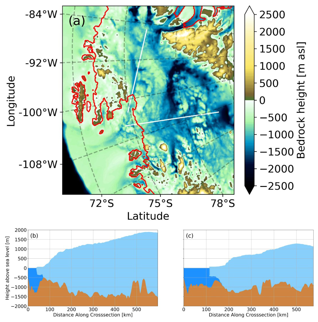
Figure 4 Regional setting of TG and PIG. (a) bedrock profile of the Amundsen Sea Embayment with the observed grounding line position, using ice thickness and bedrock height observations from Morlighem et al. (2020) in red. White lines indicate the locations of the cross sections shown below. (Bottom row) cross sections with the ice sheet shown in light blue, the ocean in dark blue, and bedrock in brown. TG in (b) and PIG in (c).

4 Results

In this section, we first discuss the modelled present-day ice sheet using the two initialization methods (Sect. 2.4). We highlight key differences and discuss implications of choices made during the initialization. Then we present the unforced future simulations, discussing their different responses to changes in basal friction and showing how these differences are related to the ice sheet geometry and buttressed ice shelves.

4.1 Initial condition evaluation

As a starting point for our forward experiments, we use the two spin-up types described in the previous sections. We evaluate the initial states here.

4.1.1 P05 initialization (P05)

Figure 5 shows the initial ice sheet state after the P05 initialization. The overall thickness bias is low. The regional thickness bias of the East Antarctic Ice Sheet (EAIS) relates to the small observed thickening in central EAIS (Smith et al., 2020), which equals a mass flux similar in magnitude to the local surface mass balance. The RMSE between modelled and observed ice thickness and modelled and observed ice surface velocity are respectively 21.10 m and 135.81 m yr⁻¹.

The modelled grounding line position (Fig. 5a) matches the observed position well, with an average error of 1.4 km. Surface ice velocities generally agree with observations except for glaciers on the Siple coast, which flow slightly too fast, and the seaward sides of the Filchner-Ronne and Amery ice shelves, where the flow is too slow. Assuming that the observed imposed $\mathrm{d}H/\mathrm{d}t$ is correct, this implies that the ice flux along flowlines in these locations decreases too quickly in CISM. Hence, to retrieve the observed geometry during the inversion, basal melt is decreased. The inverted C_c (Fig. 5c) is generally high in the interior or under slow-moving areas of the ice sheet, and low under outlet glaciers. The inverted ocean temperature perturbations (Fig. 5d) under the larger ice shelves (Filchner-Ronne, Ross and Amery) are generally close to zero with the exception of some positive corrections under the PIG, TG, and Crosson shelves in the ASE region.

Initializing the model with the P05 approach results in a dipole misfit in surface ice velocities at the TG grounding line: the Eastern Thwaites glacier flows too slowly, while the Western Thwaites glacier is too fast (Fig. S4). A similar dipole pattern emerges near the PIG grounding line, where the model overestimates velocities along the shear margins but underestimates flow along the main trunk. These discrepancies are likely due to the absence of damage representation in the shear zones, an effect that, if included, would increase the velocity gradient in the shear zone, allowing for an even more sharply defined ice stream bounded by near-stagnant ice (Lhermitte et al., 2020; Izeboud and Lhermitte, 2023).

It is important to note that the integrated grounding line fluxes shown in Figure S5 are close to observational estimates. This suggests that the slower main flow of PIG and the faster-flowing shear margins approximately balance out, resulting in a total ice flux that matches observations, an outcome that also holds for TG. While we acknowledge the surface velocity errors and their potential influence on unforced simulations, the agreement in ice fluxes supports the use of both initialization methods, P05 and P1, for future unforced model runs.

When initializing an ice-sheet model with observed ice thickness and aiming to obtain well-fitting surface velocities, it is crucial to account for present-day mass change rates, particularly in regions undergoing rapid thinning. Neglecting these rates by assuming $\frac{\partial H}{\partial t}=\mathrm{0}$, while still tuning the model to reproduce observed ice thickness and approaching present-day ice velocities, inevitably induces compensating biases. For example, dynamic mass loss substantially contributes to the ice fluxes of TG and PIG; ignoring this contribution produces a significant mismatch between observed ice thickness and surface velocity, as their product determines the ice flux. This is then compensated by artificially increasing basal friction to suppress thinning. Fundamentally, if the momentum balance and mass balance are correctly formulated and the observational data are accurate, prescribing both ice thickness and surface velocity reproduces observed mass-change patterns. Assuming zero mass change, however, forces the model to reconcile inconsistent constraints, thereby introducing systematic errors.

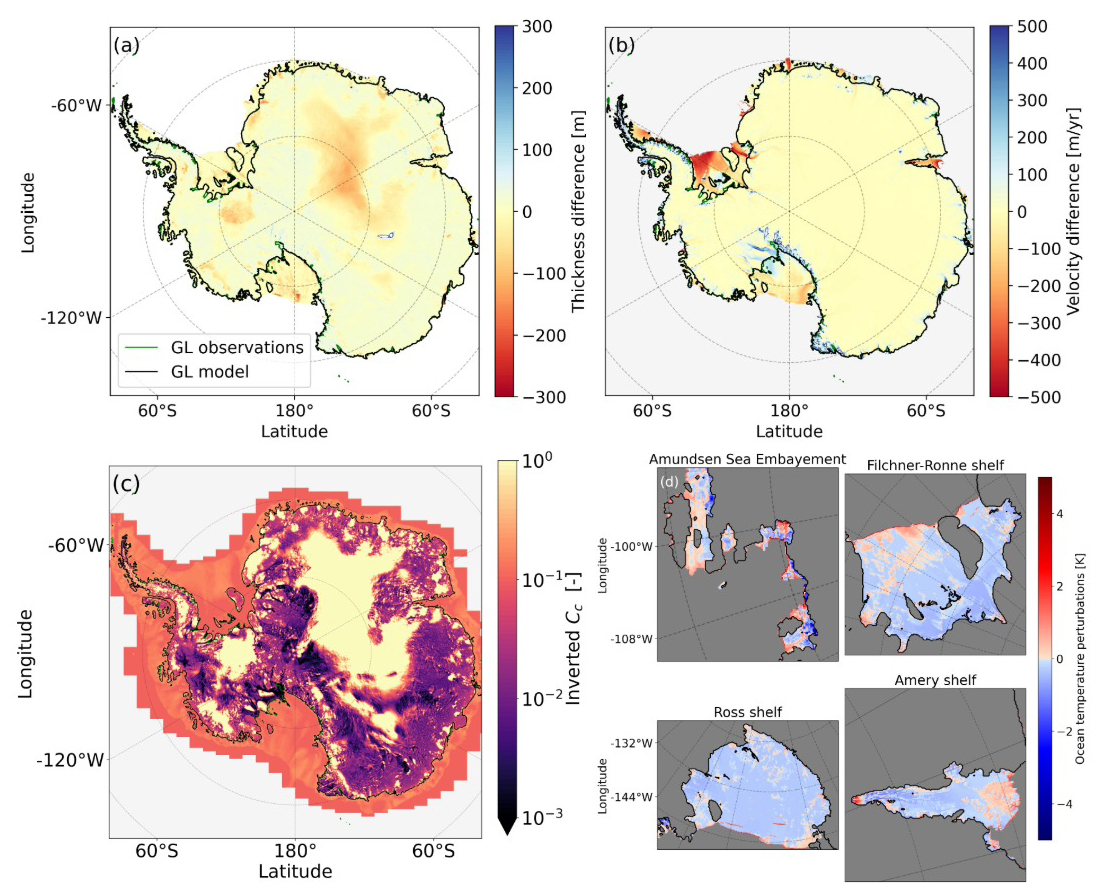
Figure 5 Modelled Antarctic Ice Sheet initialized state with the P05 inversion (DI). (a) thickness difference with respect to observations (Morlighem et al., 2020). The modelled grounding line is shown in black, and the observed grounding line in green (only visible where it does not overlap with the modelled one). (b) ice surface velocity difference with respect to the observations (Rignot et al., 2011). Positive values indicate regions where CISM overestimates the ice velocities. (c) the inverted C_c from Eq. (1) using Eq. (12). and (d) the inverted ocean temperature perturbation under the main shelves.

4.1.2 P1 Initialization (P1)

Figure 6 shows the ice sheet state after the P1 10 kyr initialization. The ice thickness and ice surface velocity are similar to the P05 initialization (RMSE thickness and velocity: 25.5 m, 136.3 m yr⁻¹). There are no large-scale differences in the inverted C_c (Fig. 6c) compared to Fig. 5c, and the inverted ocean temperature perturbations show the same pattern as in Fig. 4d. Ocean temperature perturbations are generally larger near the calving front and lower in the interior of the shelves, especially for the Filchner-Ronne and Ross shelves. The modeled grounding-line position error increases from 1.5 to 4.2 km, primarily due to a retreated grounding line relative to observations at the Bungenstock Ice Rise near the grounding line of the Filchner–Ronne Ice Shelf, and the Siple Coast. In these regions, the ice sheet rests on bedrock more than 500 m below sea level; thus, increasing p from 0.5 to 1 reduces the effective pressure beyond what the friction inversion can compensate for. As these areas are, for now, dynamically decoupled from the grounding lines of TG and PIG, we consider the p=1 initialization suitable for our purpose: evaluating the sensitivity of WAIS collapse (initiated at TG and/or PIG) to variations in the basal friction parameterization.

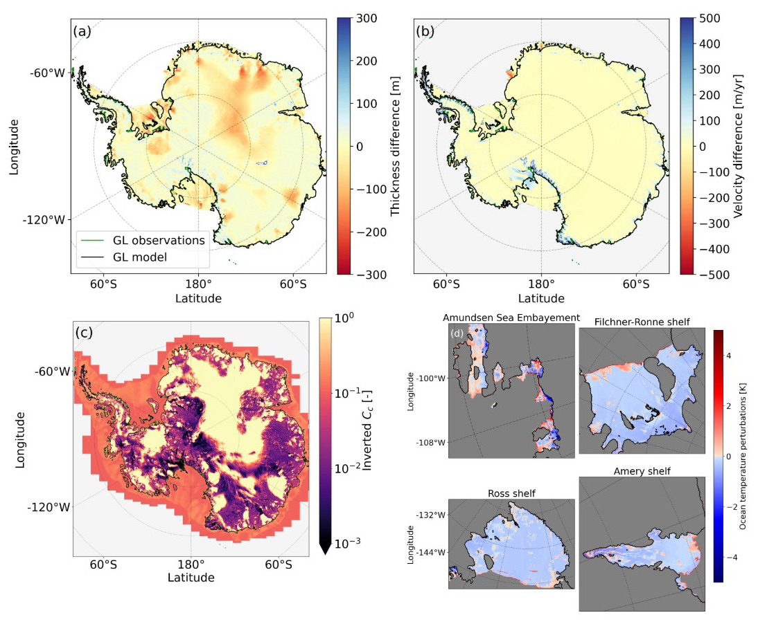
Figure 6 As in Fig. 5 but for the P1 initialization. Ice thickness difference is again between modelled and the dataset from Morlighem et al. (2020), and the ice surface velocities is the difference between modelled and Rignot et al. (2011).

Regional differences appear in the inverted parameter C_c, particularly near grounding lines, where full hydrological connectivity between the subglacial network and the ocean reduces the modeled effective pressure. For the ASE region, C_c is shown for both initializations in Fig. 7. The differences are generally small, visible mainly at the PIG grounding line and more prominently at the eastern TG grounding line. In this area, prescribing good hydrological connectivity (p=1) forces the inversion to the upper bound of C_c while still failing to maintain the observed TG grounding-line position. This leads to a slightly more retreated grounding line when comparing the P1 initialization to the P05 case, and a “patch” of a high inverted C_c.

Modeled basal friction (Fig. 8), however, is largely consistent between the two initializations except at the present-day grounding lines of TG and PIG. Given the boundary conditions (close agreement with observed ice thickness in grounded and floating ice) and the approximations used (DIVA stress balance and Glen's flow law), Fig. 7 illustrates the friction field CISM requires to reproduce the present-day AIS. The inversion compensates for parameter choices (p=0.5 vs. p=1), but as shown in Fig. 2, these choices alter the sensitivity of effective pressure to ice mass loss and, consequently, the evolving ice-sheet geometry. This will be further analyzed in the next section. As shown in Fig. 8c, a distinct band near the TG grounding line exhibits higher friction under the P1 initialization than under P05, whereas the opposite pattern occurs near the PIG grounding line. This indicates that, when P1 is chosen, CISM tends to strongly stabilize TG while destabilizing PIG. This contrast has a profound impact on the sequence of collapse observed in the continuation experiments discussed in the next section, even for the effective-pressure-independent power-law friction law.

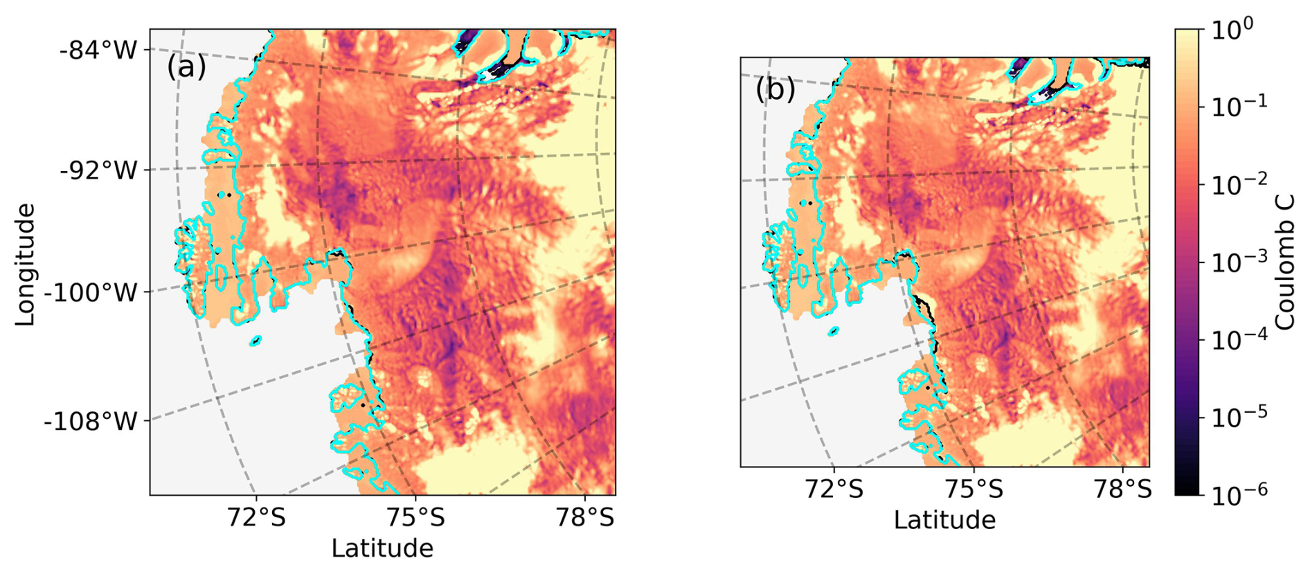
Figure 7 The inverted parameter C_c for the P05 initialization (left) and the P1 initialization (right). The observed grounding line position, derived from the observed ice thickness dataset from Morlighem et al. (2020), is shown in cyan, and the modelled grounding line position of the respective initialization is shown in black.

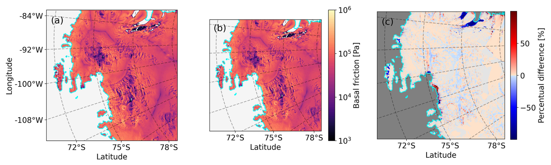
Figure 8 Basal friction of the P05 initialization (a) and the P1 initialization (b) and their percent difference (c). The modelled grounding lines are shown in cyan, derived from the observed ice thickness dataset from Morlighem et al. (2020).

4.2 Modelled unforced evolution of WAIS

Figure 9 shows the global mean sea level contribution of eight simulations initialized with the mass change rates from Smith et al. (2020). In all simulations, both PIG and TG eventually collapse, and most of the ice volume above floatation (VAF) is released to the ocean. These results are similar to those presented in van den Akker et al. (2025). In general, the simulations starting from P1 simulate a longer period of linear mass loss before the start of a steep decline in VAF. For the P05-starting simulations, two stages can be identified. These are (i) linear VAF loss similar to the present-day rate and (ii) a simultaneous collapse of PIG and TG starting around year 400. For simulations starting from the P1, three stages can be identified, in contrast to the P05 initialization (solid). These are (i) a linear decline in VAF similar to the present-day rate for the first 600 years, (ii) PIG collapse for 300 (Schoof and ZI) or 600 (power law and pseudoplastic) years, and (iii) TG collapse for approximately 200 years. The maximum rate of sea level rise during the third (TG collapse) phase differs marginally among the eight simulations (4 ± 0.7 mm GMSL per year).

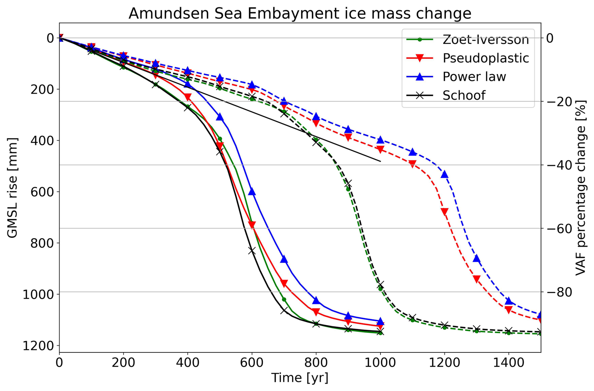
Figure 9 Sea level contributions from the ASE for four different sliding laws with basal friction and ocean temperature perturbation inversion from the P05 inversion (solid lines) and the P1 inversion (dashed lines). The ice volume above floatation [VAF] percentage change is the loss of ice that can contribute to sea level change (i.e., not already floating or present below sea level), relative to the beginning of the simulation, for the basins containing PIG and TG, respectively basins 22 and 21 in Zwally et al. (2015). The solid black line is the extrapolated present-day trend (Smith et al., 2020).

The simulations starting from P1 exhibit behavior in line with the results of Brondex et al. (2017); Brondex et al. (2019), and Sun et al. (2020): Regularized Coulomb sliding (Schoof and ZI) yields earlier and faster collapse than simulations with pseudoplastic and power law sliding. This is in stark contrast to the P05 simulations, in which the rate of glacier collapse is much less affected by the choice of the basal friction parameterization, agreeing with the results of Barnes and Gudmundsson (2022) and Joughin et al. (2024).

4.2.1 P05: Collapse mechanics and characteristics

We now discuss the results from the P05 experiments (solid lines in Fig. 9), where the collapse rate shows little sensitivity to the choice of basal friction law. Figure 10 presents elevation profiles of PIG (top row) and TG (bottom row) along the cross-sections indicated in Fig. 4. Before the collapse (year 250, first column), differences in ice sheet geometry and grounding line position across the four sliding laws are minimal for both glaciers. The final states after collapse (year 750, last column) also appear similar. However, at the midpoint of the collapse (year 500, middle column), the glacier shapes diverge for TG (panel b). For example, in the simulation using power law sliding, the grounding line has retreated roughly 75 km further than in the ZI sliding case. Notably, the ice upstream of the grounding line is thinner for the ZI sliding case compared to the power law, but the latter shows more grounding line retreat. The ZI sliding case loses more mass further inland, and the power law sliding case loses mass close to the grounding line and has a thinner ice shelf. From Fig. 9 we conclude that the integrated mass loss and SLR from the P05 sliding law simulations is very similar, but from Fig. 10 we see different geometries during the TG collapse.

This difference in geometry can also be seen in Fig. 11 which shows spatial patterns of thickness change and grounding line position. The grounding line of the power law simulation (top row) is retreated further inland compared to the ZI simulation (bottom row) during the collapse at year 500 (middle column). After 750 years, when the collapse is complete and the mass loss slows down, both simulations show a similar geometry again. These experiments show that the ZI sliding law, with lower friction far upstream of the grounding line, leads to more ice being advected from inland towards the grounding line compared to the power law. As a result, the ZI simulation shows less thinning and retreat near the grounding line, but more inland thinning, compared to the power law simulation. This means that the ZI sliding law results in a smaller but thicker ice shelf in front of the collapsing TG, with a higher buttressing potential and a greater chance to stick to pinning points.

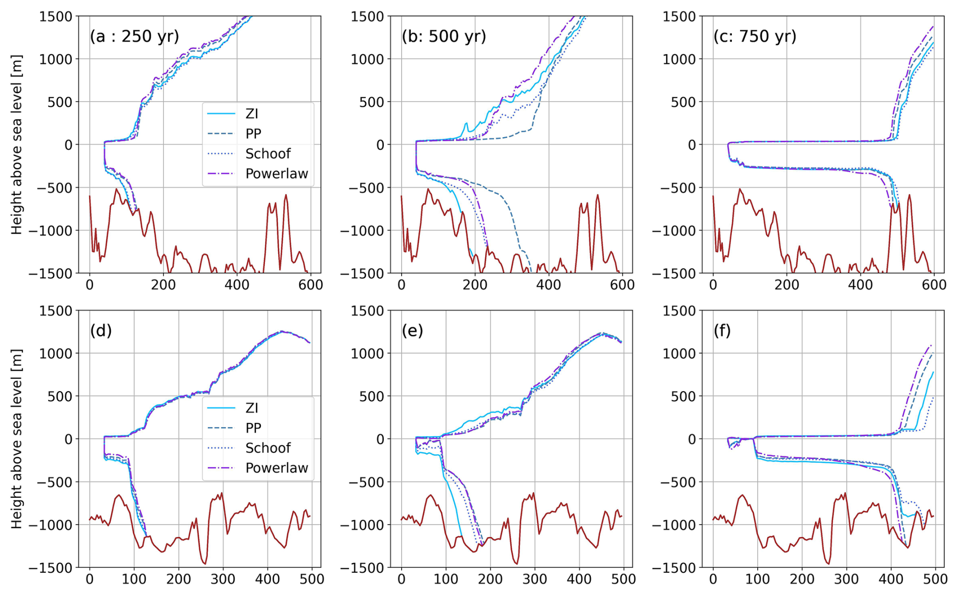
Figure 10 P05 Inversion (P05) retreat patterns for (TOP ROW) Thwaites Glacier along the cross-section shown in Fig. 4 at simulation years 250 (left column), 500 (middle column) and 750 (right column) for ZI (solid), pseudoplastic (dashed), power law (dashdot) and Schoof (dotted). Bottom row (d–f), as (a)–(c) but for Pine Island Glacier. Bedrock height asl is shown in brown.

The similarity between the simulations with Schoof and ZI sliding, and between those with power law and pseudoplastic sliding, can be explained by their similar functional relations between basal velocity and friction, shown in Fig. 1. In the rest of this section, we focus on one member from each pair: the ZI law and the power law.

Figure 11 P05 inversion (P05) spatial retreat patterns in the ASE region. Top row: ZI thickness change since the initialization at year 250 (a), 500 (b) and 750 (c), with grounding line position (green: initialized, cyan: at the timestamp of the figure). Bottom row: same for the power law.

To explain the difference in collapse mechanism but a similar VAF evolution, we analyze the buttressing of TG and PIG during the collapse. We applied both buttressing quantifications described in Sect. 2.2 to the 250- and 500-year ZI and power law simulation geometry. Both simulations show a less buttressed Western Thwaites Ice Stream and more buttressed Eastern Thwaites Ice Stream. Moving closer to the calving front decreases the buttressing number. In general, the buttressing close to the grounding line is stronger for the ZI sliding law, according to this method. Little difference can be seen in the confined Pine Island Glacier in both simulations.

The right side of Fig. 12 shows the acceleration factor during the shelf-removal experiments at years 250 and 500, comparing ZI sliding (left column) and power law sliding (right column). Following the removal of the ice shelves, grounded ice in the ZI simulation accelerates rapidly, especially at the TG grounding line and further inland, much more so than in the power law case. Two primary mechanisms can slow down a retreating marine-terminating glacier like TG: buttressing and basal friction. At year 500, buttressing at the TG grounding line is stronger in the ZI simulation than in the power law case, as indicated by the higher buttressing numbers. Despite this, the acceleration response to shelf loss (Fig. 12c,d,g,h) is greater in the ZI case. This is because, in the power law case, basal friction increases with velocity (as shown in Fig. 1), limiting the glacier's speed-up and upstream propagation of the acceleration. In contrast, the ZI simulation exhibits less frictional resistance and thus stronger acceleration. This is further examined in Figs. S6 and S7, where we show the ice velocity increases due to ice shelf removal when the ZI geometries are tested using power law sliding, and the power law states are tested using ZI. To change the sliding law while retaining the same ice sheet state and velocities prior to ice shelf removal, we used again the procedure described in the Supplement. Now, the power law states with ZI basal friction have the largest velocity increases (Fig. S7), even larger than these for the ZI state using ZI (Fig. 12e, g). Conversely, the ZI states with a power law lead to the lowest velocity increases (Fig. S6), which are also lower than these for the power law state using the power law (Fig. 12f, h). We conclude that, during the TG collapse, buttressing is the primary braking mechanism in the ZI case, whereas increased basal friction dominates in the power law case. Interestingly, due to the specific bed geometry of TG and the conditions in the unforced simulation, both scenarios produce a similar contribution to global mean sea level rise – though driven by different mechanisms.

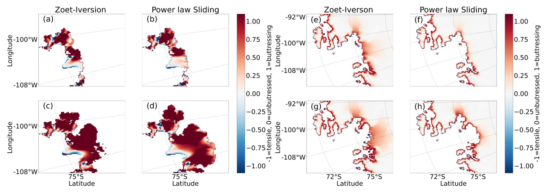
Figure 12 Buttressing number and acceleration number for the P05 simulations (left four panels) Buttressing number calculated over the floating ice shelves at 250 years (top row) and 500 years (bottom row), for the ZI sliding law (left column) and the power law (right column). (Right four columns) acceleration number after removing the ice shelves at 250 years (top row) and 500 years (bottom row), for the ZI sliding law (left column) and the power law (right column). Note the different zooms of the four panels on the left and the four panels on the right. This is done to preserve detail in the left four panels.

With ZI sliding in our P05 continuation simulations during the TG collapse, the dominant resistive force is buttressing, whereas with power law sliding, the dominant resistive force is basal friction. There is a compensation effect in the continuation experiments because the ice shelf in all runs is allowed to persist (no calving front retreat, no forcing applied other than the present-day calibrated ocean temperatures). If the shelf were significantly weaker because of either calving or ocean warming, we would expect the ZI law to yield faster collapse, since the buttressing would not be present to compensate the lower friction.

4.2.2 P1: Collapse mechanics and characteristics

In contrast to the P05 experiments, the P1 simulations show a strong sensitivity to the choice of basal friction law in terms of integrated ice mass loss and GSML contribution. Also, the collapse of the ASE occurs later, beginning around year 800 in the ZI case and around years 1000–1200 in the power law case, and it follows a different pattern. Instead of transitioning directly from present-day-like mass loss rates (∼ 0.3 mm yr⁻¹) to full collapse rates (∼ 3 mm yr⁻¹), there is an intermediate phase with mass loss rates of approximately 1–2 mm yr⁻¹. This transitional phase is driven primarily by the collapse of PIG, which occurs independently of TG in the P1 simulations.

Figure 13 shows a typical snapshot from the collapse phase (the first inflection points in Fig. 9) in both initializations. In the P05 simulations, TG collapses first. In contrast, PIG collapses first in the P1 simulations, while TG is temporarily stabilized on a bedrock ridge about 40–50 km upstream of the present-day grounding line (white line in Fig. 13). TG reaches this grounding line quickly, before PIG's grounding line starts to recede, but then stabilizes for 800–1000 years. Once PIG has retreated sufficiently and starts to draw ice from the Thwaites basin, TG starts to collapse. Thus, unlike the P05 simulations, PIG initiates ASE deglaciation when using P1.

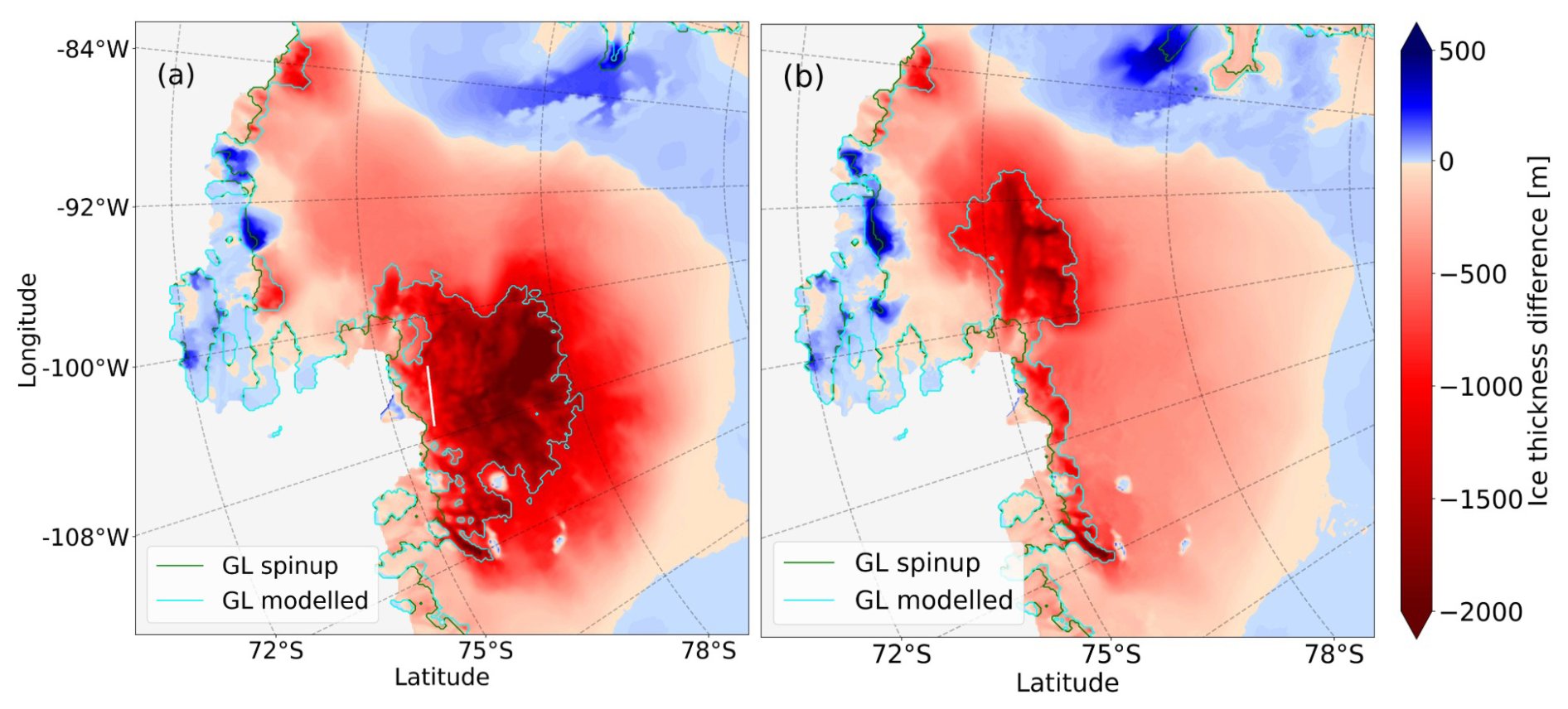
Figure 13 Start of Amundsen Sea ice collapse in simulations with the P05 (left) and P1 (right). Colors indicate the ice thickness difference with respect to the initialization, and the modelled grounding line is shown for the initialization (green) and continuation (cyan). The time snapshots of the left and right panels are respectively for years 575 and 850. Results shown here are from the ZI sliding simulations, but results are similar for the power law simulation.

PIG often collapses more slowly than TG in our simulations. This is shown in Fig. 14. A typical collapse phase of the PIG in these simulations lasts about 300 years when using a ZI sliding law, and up to 800 years when applying power law friction. During this time, the ice sheet loses about 50 cm in GMSL equivalent. Since we do not apply surface melting, all losses of grounded ice happen through advection across grounding lines. A large ice flux at the grounding line initially thickens and strengthens the ice shelf. For TG in the P05 simulations, this has a braking effect: a thicker, stronger and more buttressed ice shelf slows the upstream flow and reduces the ice flux through the grounding line. For PIG, the increased grounding line flux apparently does not increase the buttressing enough to slow the collapse.

Figure 14 Mass loss shown separately for PIG (left, a) and TG (right, b), for both initializations (solid is P05 and dashed is P1) and for two sliding laws.

5 Discussion

Our study is consistent with studies arguing that different basal friction parameterizations cause significantly rates of ice loss (Brondex et al., 2017; Sun et al., 2020; Brondex et al., 2019), and also with studies that claim the opposite (Barnes and Gudmundsson, 2022; Wernecke et al., 2022), although the latter two studies focus on shorter timescales (∼ 100 years) and feature much less grounding line retreat than our study (e.g., no WAIS collapse). We argue that sensitivity to the sliding law depends on the geometric evolution during the retreat phase, e.g. on whether newly formed ice shelves can survive and provide buttressing. In our cases, the geometric evolution is sensitive to modelling choices made during initialization, even though the two initial states are very similar. This study was inspired by Berends et al. (2023), who showed that obtaining a similar initial state does not necessarily lead to the same forced retreat in idealized experiments.

The connection between buttressing and basal friction during TG collapse in the P05 simulations hinges on the survival of the ice shelf that forms during grounding-line retreat. This is in turn determined by ice flux across the GL and available pinning points, but also on the basal melt and calving rates. With respect to calving, we apply a no-advance calving front at the present-day position. Theoretically, the calving front can move inland, but we use a conservative limit of 1 m ice thickness before ice is removed. In practice, this rarely happens. Using a physically-based calving law would likely increase calving rates as the ice thins and the grounding line retreats, and might reduce the buttressing feedback.

With respect to basal melt rates, we apply the ISMIP6 basal melt parameterization (Seroussi et al., 2020) with thermal forcing data from Jourdain et al. (2020). Although this approach yields basal melt fluxes in agreement with observations and other model studies (see van den Akker et al., 2025), other approaches – such as including a coupled cavity-resolving (regional) ocean model or a sub-model capturing cavity flow like PICO (Reese et al., 2018b) – could result in basal melt rates that are more physically based and lead to different results. The ISMIP6 parameterization lacks freshwater feedbacks such as the reduced formation of Antarctic Bottom Water (Williams et al., 2016) and cooling of the sea surface (Bintanja et al., 2015). Increases or decreases in future basal melt rate will moderate the buttressing effect of the newly formed shelves. Resolving basal melt rates with a model for ocean circulation in cavities could be an interesting topic for future research.

This study accounts for subglacial hydrology only in a simplified way. We parameterize the effective pressure N according to Leguy et al. (2014), where we assume that N is reduced near grounding lines because of a connection between the subglacial hydrology network and the ocean. While this captures some aspects of including a subglacial hydrological system (e.g. lowering basal friction in areas close to grounding lines), it does not simulate a complex hydrological network as was done, for example, by Kazmierczak et al. (2024) or Bradley and Hewitt (2024). Including a more complex hydrological network and coupling it via the effective pressure to the basal friction would likely alter our results because hydrological processes are now incorporated in the basal friction inversion. Taking those out of the inversion will likely change the inverted fields considerably, and therefore also our projections.

When future ocean warming is applied, the resulting ASE ice shelves are expected to be much smaller. As a result, the buttressing effect that moderates retreat in the ZI simulation would be reduced, likely leading to greater projected GMSL rise compared to the power law case. Therefore, the results presented here are specific to the CISM model, the initialization techniques used to reproduce present-day mass loss, and the absence of any future forcing. Follow-up studies are needed to evaluate whether our conclusions hold under different scenarios, such as sustained ocean warming or through transient calibrations designed to reproduce historical mass loss trends (e.g. Goldberg et al., 2015).

At first glance, it may seem counterintuitive that simulations initialized with p=0.5 produce a faster WAIS collapse than those with p=1. Although the p=1 initialization generally yields lower effective pressure, this is largely compensated during inversion. As shown in Fig. 2, however, the sensitivity of effective pressure to ice mass loss is greater in the P05 initialization, meaning that effective pressure decreases more sharply when ice is removed. Because C_c remains fixed during continuation simulations, basal friction declines more rapidly (for comparable basal ice velocities) in the p=0.5 case, driving faster retreat.

This behavior also occurs under the effective-pressure–independent power law, indicating that the sequence of collapse (PIG first vs. TG first) is not dictated by differences in basal-friction sensitivity, but rather by the specific C_c and basal-friction patterns established during initialization. If sensitivity alone were the controlling factor, the power-law simulations from the P05 and P1 initializations would exhibit similar retreat patterns, which is not observed.

At present, it is not possible to determine whether p=0.5 or p=1 is more realistic for the effective pressure beneath marine-grounded ice, due to the lack of direct observations of basal pressure, friction, or the subglacial hydrological system of the AIS. Both approaches capture a reduction in basal friction near grounding lines due to ocean water pressure, and both yield comparable initial states, yet they produce divergent long-term responses.

6 Conclusion

In this study, we conduct Antarctic Ice Sheet simulations initialized to be consistent with present-day mass loss rates. We use two initializations with different treatments of the ice effective pressure on bedrock below sea level. These two initializations lead to distinctive ice sheet evolution when run forward with present-day climate forcing. In the first case, Thwaites Glacier collapses first and shows compensation between basal friction and buttressing: increased ice velocities and grounding line fluxes can increase the buttressing capacity of the ice shelf downstream. This makes the future projections insensitive to the specific basal friction law used. In the second case, Pine Island Glacier collapses first, without a connection between basal friction and buttressing. In the absence of strong buttressing, power law friction slows down the eventual collapse. As a result, the sensitivity of our modelled Antarctic Ice Sheet to the choice of basal friction parameterization is determined by the order of collapse, which in turn is determined by the initialization. Applying the inverted present-day ocean forcing results in the collapse of both the Thwaites and Pine Island glaciers, but small differences in the initialization procedure introduce an uncertainty in its timing of about 500 years.

This analysis explains why CISM can generate evolution with either strong or weak sensitivity to the choice of basal sliding law, depending on whether ice shelf buttressing provides a negative feedback on the grounding line fluxes. Carrying out similar experiments with other ice sheet models will enhance our understanding of why some simulations (Brondex et al., 2017; Sun et al., 2020; Brondex et al., 2019), are more sensitive to changes in basal friction laws than others (Barnes and Gudmundsson, 2022; Wernecke et al., 2022), and possibly lead to similar conclusions. One way to address this issue is through standardized tests (e.g. MISMIP+ for different sliding laws). Also, projections could start from an ensemble of many initializations, all done with different model choices. Explorations with more realistic treatments of calving and ocean thermal forcing could also be illuminating. Finally, new (depth) observations on the relative strength of sliding- versus deformation-dominated flow would reduce the degrees of freedom now present in the initialization of ice sheet models.