Stabilizing feedbacks allow for multiple states of the Greenland Ice Sheet in a fully coupled Earth System – Ice Sheet Model

It remains uncertain at which volume threshold the Greenland Ice Sheet (GrIS) mass loss will become irreversible under continuous warming and if the GrIS could regrow under pre-industrial (PI) CO₂ concentrations. We use a newly developed comprehensive fully-coupled climate–ice sheet model to explore a potential multistability of the GrIS. This model system is more complex, includes interactive GrIS and Antarctic Ice Sheets (AIS) and more critical feedbacks relevant for the stability of the GrIS than previously used models. Our steady-state simulations indicate at least four steady states under PI CO₂ concentrations: a state with a large GrIS, similar to the PI and current state, and three smaller states with GrIS volumes of about 50 %, 30 % and 20 % of the PI volume. These steady states are stable through the interplay of several feedback processes. The most important ones are the melt–elevation and melt–albedo feedback. We also show that interactions between the GrIS and the AIS impact the transient behavior of the GrIS. Our results highlight the importance of fully-coupled climate–ice sheet feedbacks in maintaining multiple steady states of the GrIS. Such multistability has implications for assessing the consequences of global warming. Our simulations indicate that if the GrIS volume drops below a critical threshold of 83 %–70 % of its PI volume, at least half of its current volume will be irreversibly lost even if we return to global PI temperatures through a reduction in CO₂ concentrations.

1 Introduction

The Greenland Ice Sheet (GrIS) is a critical component of the Earth system and has undergone strong warming in recent decades (McGrath et al., 2013; Jiang et al., 2020; Hörhold et al., 2023). The GrIS has also been losing mass at accelerating rates, mainly due to an increase in surface melt (Shepherd et al., 2020). Future projections indicate that continued warming could lead to a substantial mass loss (Pattyn et al., 2018), with profound implications for regional climate dynamics (e.g., Toniazzo et al., 2004; Junge et al., 2005; Davini et al., 2015; Andernach et al., 2025) and the global-mean sea level (Morlighem et al., 2017; Aschwanden et al., 2019; Goelzer et al., 2020). Under sustained warming, the GrIS might even cross a tipping point, beyond which the ice sheet becomes unstable due to self-amplifying feedbacks (Pattyn et al., 2018; Boers and Rypdal, 2021; Bochow et al., 2023; Petrini et al., 2025). This implies that the GrIS may transition into a new steady state. To explore the stability of the GrIS and to understand the climate conditions that constrain potential multiple steady states of the GrIS, we take advantage of the newly developed Max Planck Institute for Meteorology Earth System Model (MPI-ESM) coupled to the modified Parallel Ice Sheet Model (mPISM) in a bi-hemispheric set-up and the glacial isostatic adjustment (GIA) model VIscoelastic Lithosphere and MAntle model (VILMA;  Mikolajewicz et al., 2025). The bi-hemispheric setup allows us to also investigate the role of the Antarctic Ice Sheet (AIS) for the stability of the GrIS.

Theoretically, if the GrIS were to disappear, it could regrow over millennia under certain climate conditions (Letréguilly et al., 1991; Robinson et al., 2012; Solgaard and Langen, 2012; Höning et al., 2023). A full regrowth of the GrIS has been shown to be possible under present-day (PD) climate conditions due to a monostability of the GrIS in studies using a stand-alone Ice Sheet Model (ISM; Letréguilly et al., 1991; Lunt et al., 2004). Monostability means that a system (e.g., the GrIS) experiences only one stable state under the same climate conditions. It is in contrast to multistability, where a system can experience more than one stable state under the same climate conditions depending on its history. Such multistability has been shown in coarse General Circulation Model (GCM) modeling studies, in which a disintegration of the GrIS would be irreversible and a regrowth under a PD climate unlikely, as summer temperatures are too high in absence of the GrIS to form a perennial snow cover (Crowley and Baum, 1995; Toniazzo et al., 2004). It is also possible that the GrIS would only regrow to a smaller size than at PD (Ridley et al., 2010; Langen et al., 2012; Gregory et al., 2020). This indicates that the GrIS might be multistable under specific climate conditions. Differences in the identification of the existence and the number of multiple steady states of the GrIS across earlier studies may stem from differences in the model complexity, the coupling between the ISM and other components of the climate model as well as the inclusion of feedback mechanisms between ice sheets and the Earth system. Feedbacks can either enhance the melting of the GrIS (positive feedback) or stabilize it, by slowing down the melting or even favoring ice sheet growth (negative feedback).

Important positive feedbacks include the melt–elevation feedback, which describes the enhancement of ice sheet melt through the lowering of the surface elevation and exposure to warmer surface temperatures following an initial melt, and the melt–albedo feedback, which is associated with an increased surface melt due to more shortwave absorption at the surface in response to ice melt (Fyke et al., 2018). Studies that disregard this interaction do not accurately capture mass changes of the GrIS (Zeitz et al., 2021) and likely underestimate the mass loss and overestimate the regrowth of the GrIS. Furthermore, changes in the elevation can impact atmospheric circulation patterns (Dethloff et al., 2004; Lunt et al., 2004; Petersen et al., 2004; Toniazzo et al., 2004; Junge et al., 2005; Langen et al., 2012; Andernach et al., 2025). A different precipitation pattern or the advection of different air masses may then feed back onto the GrIS. Furthermore, Langen et al. (2012) showed that an emerging Föhn effect on the lee side of a smaller GrIS in the southeast can inhibit an expansion of a small ice sheet. The melt–albedo feedback significantly increases ice loss, as demonstrated in an analysis of the future evolution of the GrIS under various warming scenarios (Zeitz et al., 2021). Additionally, Gregory et al. (2020) found that the steady states of the GrIS under PI climate conditions are highly dependent on the snow albedo settings. For example, a low albedo only allowed for a restricted regrowth when starting with no ice, whereas a high albedo supported a full recovery. Neglecting changes in the surface albedo as the ice melts could therefore overestimate ice sheet regrowth. As the surface albedo is highly dependent on the vegetation cover and the growth of vegetation has been shown to inhibit glaciation (Stone and Lunt, 2013), disregarding vegetation feedbacks might also overestimate a regrowth of the GrIS.

Several negative feedbacks have been suggested that compete with the positive feedbacks, having the potential to counteract ice loss (Zeitz et al., 2022). A melting ice sheet reduces the load on the bedrock, allowing for isostatic uplift, which raises the overall ice sheet elevation and thus the net surface mass balance (SMB). However, the GIA acts on long timescales of centuries to millennia. Another cooling effect on Greenland is freshwater release from GrIS melting into the North Atlantic. The freshwater alters ocean density and circulation patterns in the regions of deep convection (Stouffer et al., 2006; Weijer et al., 2012; Böning et al., 2016; Li et al., 2023), which can slow down the Atlantic Meridional Overturning Circulation (AMOC). The reduced northward heat transport into the North Atlantic and the Arctic (Caesar et al., 2018) can stabilize the GrIS. Lastly, iceberg discharge from the GrIS lowers the heat release of the ocean towards the atmosphere and cools Greenland by increasing sea-ice thickness (Bügelmayer et al., 2015).

Changes in the GrIS volume potentially impact the AIS through modifications in the sea level and ocean circulation. It has been suggested that Northern Hemisphere sea-level forcing caused grounding line changes in the marine-based sectors of the AIS during the geological past (Denton and Hughes, 1983; Denton et al., 1986; Gomez et al., 2020). Southern Hemisphere sea-level forcing could in turn feed back onto the GrIS. However, the sensitivity of the GrIS to sea-level rise is comparatively low, as its bedrock is mostly situated above sea level (Wunderling et al., 2024a). Yet, it remains an open question how the AIS might influence the steady states of the GrIS. These interactions point towards the importance of a two-way coupling between ice sheets and every other component of the climate system for the realistic representation of GrIS dynamics.

In view of the significant environmental and social impact of a disintegrated GrIS, it is important to better understand how the GrIS might behave under future warming. Considering or disregarding climate–ice sheet feedbacks creates uncertainty about the likelihood of a full regrowth of the GrIS after disintegration and the number of steady states. Previous studies have shown that state transitions of the GrIS can be (de)stabilized by the interaction with other climate components (Wunderling et al., 2024b). Although multistability of the GrIS has been demonstrated by previous studies using simplified regional models (Robinson et al., 2012), intermediate-complexity models (Höning et al., 2023), AGCM-only couplings (Gregory et al., 2020) or AOGCM set-ups (Ridley et al., 2010), these studies neglected some (de)stabilizing interactions with other climate components (e.g., AMOC adjustments, vegetation and GIA feedback). To our knowledge, only one study of the stability of the GrIS exists that accounted for the aforementioned feedbacks by using an ESM coupled to an ISM (Vizcaíno et al., 2008). While this study found a bistability of the GrIS under PI conditions, its analysis focused mainly on feedback mechanisms between ice sheets and the climate and not on the climate conditions that determine the obtained steady states. Further, the spatial resolution of their model was relatively coarse, which may have affected the ability to capture all aforementioned processes. Hence, to this date, the role of many interactive feedbacks in shaping the GrIS's stability regimes remains uncertain, highlighting the need for further investigation using fully coupled climate–ice sheet models.

In the present study, we close this methodological and knowledge gap by investigating the stability of the GrIS under PI CO₂ concentrations with a novel version of MPI-ESM coupled to mPISM and VILMA (Mikolajewicz et al., 2025). Further, we identify which feedbacks or combination of feedbacks constrain each steady state of the GrIS. As our model also includes an interactive AIS, it enables the analysis of interactions between the GrIS and the AIS and its impact on the GrIS's stability for the first time.

In the following section, the model components are described along with the experimental design. In Sect. 3, we present the steady states of the GrIS found with our model setup as well as the climate conditions constraining them. Further, we investigate interactions between the GrIS and AIS and their role in constraining the GrIS's steady states. In Sect. 4, we summarize and discuss the findings with respect to previous studies, followed by the conclusions in Sect. 5.

2 Methods

To investigate how many steady states of the GrIS exist, we compiled a set of steady-state simulations initialized with different volumes of the GrIS under PI greenhouse gas concentrations. Additional experiments serve to understand feedbacks of the ice sheets with the ocean and how the steady states are influenced by the AIS.

2.1 Model system

The simulations were run with the fully-coupled atmosphere–ocean–vegetation–ice sheet–solid earth model MPI-ESM/mPISM/VILMA (Mikolajewicz et al., 2025). It uses the coarse resolution MPI-ESM version 1.2 (Mikolajewicz et al., 2018; Mauritsen et al., 2019). The ESM consists of the ECHAM6.3 spectral atmospheric model (Stevens et al., 2013) at a T31 horizontal resolution (approximately 3.75°) and 31 vertical levels, the JSBACH3.2 land surface vegetation model (Raddatz et al., 2007) and the MPIOM1.6 primitive equation ocean model (Marsland et al., 2003; Mikolajewicz et al., 2007; Jungclaus et al., 2013) with a nominal resolution of 3°. The ESM is coupled to the ISM mPISM (Ziemen et al., 2019) based on PISM version 0.7.3. mPISM has a horizontal resolution of 10 km in the Northern Hemisphere and Antarctica. At the atmospheric boundary, the ESM and PISM are coupled through an energy balance model (EBM), which calculates a yearly SMB on 24 height levels based on hourly atmospheric data. This data is then interpolated onto the ice sheet surface (for details see Kapsch et al., 2021). At the ocean interface, salinity and temperature averages from 203 to 523 m are used to extrapolate the ocean conditions underneath the ice shelves and to estimate basal melt (Mikolajewicz et al., 2025). Changes in the solid Earth and the change in relative sea level due to a redistribution of ice and water are computed with the global model VILMA (Martinec et al., 2018). The model also includes an Eulerian iceberg model (Erokhina and Mikolajewicz, 2024) as well as interactive topography, bathymetry, land–sea mask (Meccia and Mikolajewicz, 2018) and adaption of river routing directions (Riddick et al., 2018). Thus, the model system accounts for the melt–elevation, melt–albedo and GIA feedback, as well as interaction between the ice sheets with the dynamic atmosphere, the ocean, the land surface and vegetation and icebergs. For more details on the model system refer to Mikolajewicz et al. (2025), who used a similar model system. Our model version differs from Mikolajewicz et al. (2025) in that we included additional features, such as an updated parameter tuning and an expanded ocean model grid that extends the GR30 grid of Mikolajewicz et al. (2025) across the land–sea boundaries of Greenland and Antarctica. An expanded grid is required to accurately simulate ocean dynamics beneath newly exposed ocean grid cells as the ice sheets retreat. mPISM and VILMA are asynchronously coupled to the ESM. This means, that following 10 years of simulated climate with MPI-ESM, mPISM and VILMA run with the repeated 10 year ESM forcing for 100 years. The simulated ice sheet geometry is then used as input into MPI-ESM. This allows for the simulation of long timescales that are necessary to capture the slow response times of ice sheets (Cuffey and Paterson, 2010). At the end of the 100 year-long ISM cycle, the averaged meltwater and iceberg fluxes are transferred to the ESM. The asynchronous coupling could have an influence on the timing of transitions in the ice sheet due to the long response time scales of the ocean. Focusing on the equilibrated steady states, the asynchronous coupling method should have no significant impact on the results.

2.2 Experimental design

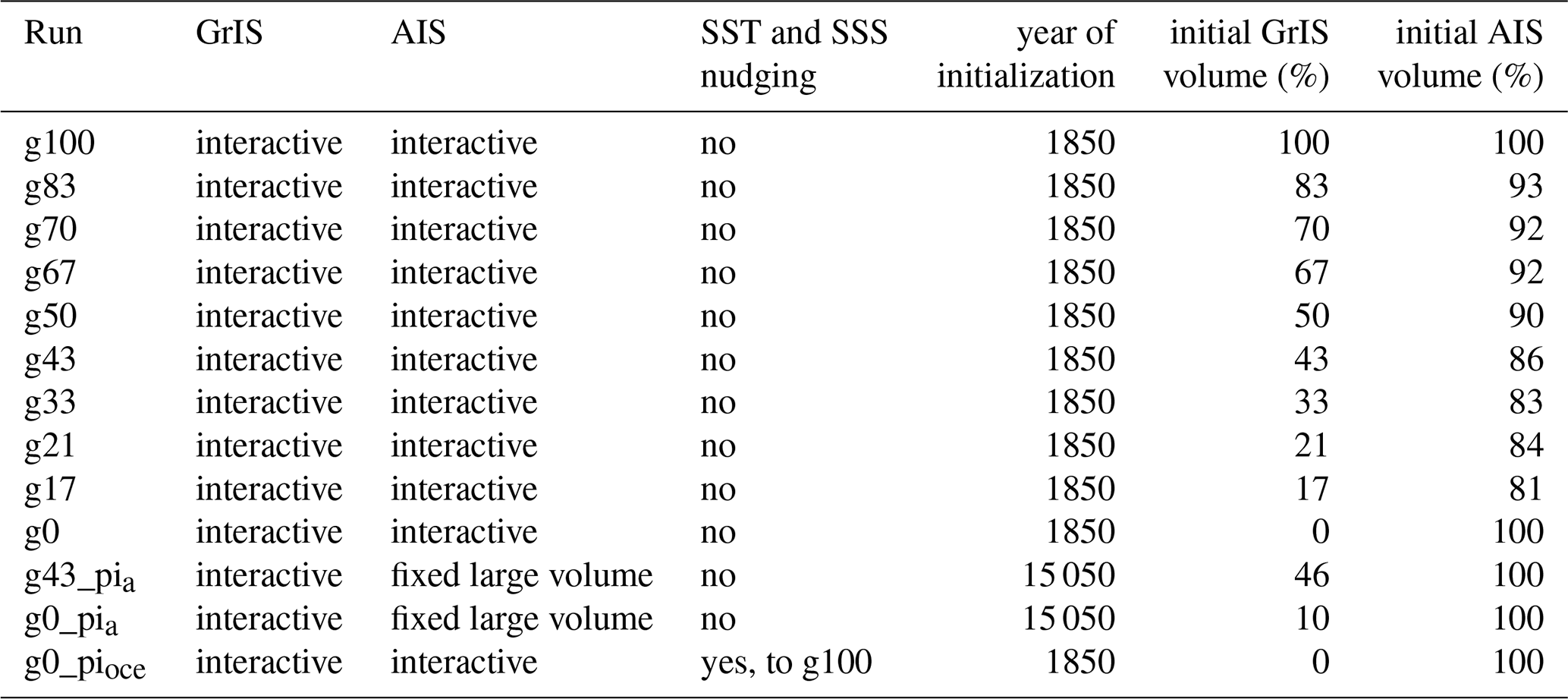
Aiming to study the existence of potential multiple steady states of the GrIS, we performed ten simulations that started from different GrIS volumes (0 %, 17 %, 21 %, 33 %, 43 %, 50 %, 67 %, 70 %, 83 % and 100 % of the PI value). These were run until equilibrium under prescribed constant PI greenhouse gas concentrations (CO₂ of 282.59 ppm, CH₄ of 711.09 ppb and N₂O of 270.28 ppb; Köhler et al., 2017) and orbital parameters (Berger and Loutre, 1991). Figure A1a–j in the Appendix displays the initial ice thickness map and the initial volume of each simulation.

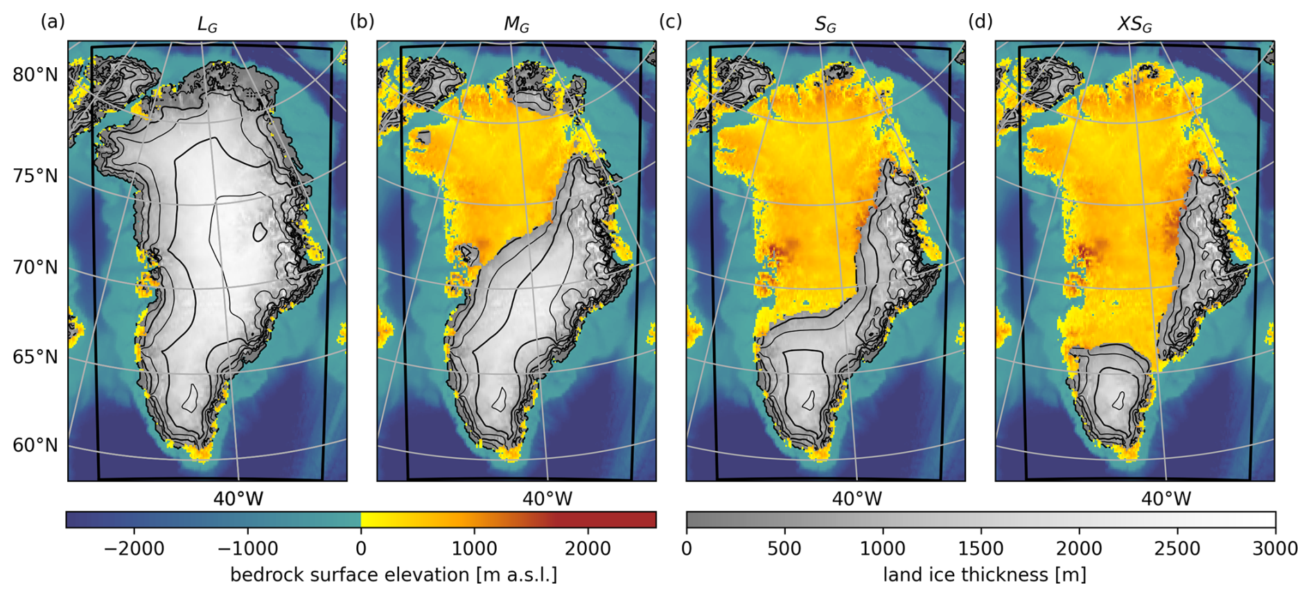
Figure 1 Maps of ice thickness in meters of the final steady state GrIS volumes overlaid on the surface bedrock in meters above sea level ($\mathrm{m}\mathrm{a}.\mathrm{s}.\mathrm{l}.$) for the respective state. Ice thickness contours are delineated at 500 m intervals. The black frame shows the area that has been integrated to compute the GrIS volume in Fig. 2.

The simulation started at 100 % is an equilibrium run with a steady-state PI GrIS and PI AIS that was initiated from an equilibrated asynchronous fully-coupled spin-up simulation. Note that the PI state of both ice sheets is similar to PD. This simulation is referred to as g100, where “g” refers to the GrIS and “100” indicates its initial volume, and serves as reference PI simulation. The GrIS volume in g100 is only 1.7 % larger than the volume obtained from the IceBridge BedMachine of the NASA National Snow and Ice Data Center (NSIDC) Distributed Active Archive Center (Morlighem et al., 2022). In the simulation with 0 % initial GrIS volume (g0), we initially removed the GrIS in g100 and let the underlying surface bedrock adjust isostatically. We continued the run until the GrIS reached a new equilibrium under PI CO₂ that is significantly smaller than its PI volume. The remaining initial GrIS volumes were obtained by branching off simulations at different volumes from a run in which this small GrIS in g0 continued to regrow under progressively decreasing CO₂ concentrations. We continued these simulations under PI CO₂ concentrations until reaching a new equilibrium or converging to the steady state of another equilibrium simulation. In all simulations the bedrock adjusted interactively to the changing ice sheets. Note that the bi-hemispheric model set-up allows for changes in the AIS. Hence, responding to the changes of the GrIS, the AIS also changes significantly. The initial ice distributions of the AIS are illustrated in Fig. A2 in the Appendix.

To explore the interactions between the GrIS and the AIS, and the impact of the AIS on the steady states of the GrIS, we branched off simulations from the steady-state simulations initialized at 0 % and 43 % (g0 and g43, respectively) in year 15 050 (Appendix Fig. A1k and l) and prescribed a constant PI AIS volume. These simulations are referred to as g0_pi_a and g43_pi_a, where pi_a stands for constant PI AIS. An additional sensitivity experiment performed to study feedbacks with the ocean will be introduced throughout the analysis. If not stated differently, we analyze the means over the final 1000 years of each simulation. The final steady-state simulations and the sensitivity experiments are summarized in Table 1.

Table 1 Overview of the simulations, including their names, which are indicative of the initial GrIS volume, whether an interactive GrIS and/or AIS was used, whether nudging of SST and SSS was applied, the year of initialization and the initial volume of the GrIS and AIS. The sensitivity experiments will be further explained throughout the analysis in Sect. 3.

With the aim of disentangling the feedbacks that constrain each steady state, we performed additional sensitivity experiments. These separate the impact of the different factors, including surface elevation, GIA, glacier mask and albedo, precipitation, and the ocean, on the stability of the steady states. To obtain the contribution of the surface elevation, we mapped the last 100 years of our 3D SMB data of each state onto the surface topography of the neighboring state. This yields which impact the total elevation effect has on the steady states. This effect is composed of the elevation change due to the ice-thickness change and the counteractive isostatic adjustment of the underlying bedrock. To separate the effects of the ice-thickness difference and GIA, we compared the elevation changes due to the ice thickness and GIA difference to the total elevation changes. We then linearly scaled their contributions to the SMB effect of the total surface elevation effect. The effect of the glacier mask and surface albedo has been isolated by running simulations of each steady state with MPI-ESM for 1000 years, using the glacier mask of the neighboring state, while keeping the ice sheets constant. We derived the SMB fields from these simulations using the EBM. To analyze the impact of the precipitation, we retained all conditions of each individual state, but scaled the precipitation fields to the ones of the neighboring state of the last 100 years (e.g., climate of one state but with precipitation of the next larger state to force the EBM), to yield the same climatology as the neighboring state. We then ran the EBM with the modified 100 years of atmospheric data to derive the precipitation effect on the SMB. Lastly, the ocean contribution on the stability of each state is filtered out by running MPI-ESM for 200 years started from the end of each steady state and nudging the sea-surface temperature (SST) and sea-surface salinity (SSS) towards the averaged last 200 years of the neighboring states, while keeping the ice sheets constant. In all cases, the resulting last 100 years of SMB is compared to the original SMB of each steady state. These experiments indicate how each feedback process restricts the mass gain or loss of the GrIS states.

3 Results

3.1 The steady states of the GrIS

Initialized from different initial ice sheet volumes (Fig. A1a–j), we obtain four steady states of the GrIS (Fig. 1): a large, a medium, a small and a very small state (L_G, M_G, S_G and XS_G, respectively). L_G corresponds to the PI state with a maximum ice thickness of about 3200 m in eastern Greenland (Fig. 1a). In L_G, the GrIS holds an ice volume of about 3.0 × 10¹⁵ m³, corresponding to 7.3 m of sea-level equivalent (SLE). In XS_G, the GrIS is split into two separate parts that are confined to the eastern and southern mountain ranges, reaching elevations of up to 2600 and 1600 m, respectively (Fig. 1d). The eastern part grows to a maximum ice thickness of 2300 m, while the southern part has a maximum ice thickness of about 2000 m. The GrIS in XS_G retains 20 % of its PI volume, equivalent to about 0.6 × 10¹⁵ m³ or 1.4 m SLE of ice. In the next larger state S_G, the southern and eastern parts of the ice sheet are connected by a narrow stretch of ice and form one single small ice sheet (Fig. 1c). In S_G, the GrIS has a maximum thickness of about 2400 m. Its final volume amounts to about 30 %, which corresponds to 0.8 × 10¹⁵ m³ or 2.1 m SLE. In the last state M_G, a medium-sized ice sheet is present with a final volume of about 50 %, equivalent to 1.4 × 10¹⁵ m³ or 3.5 m SLE (Fig. 1b). Compared to S_G, the ice sheet in M_G extends further northwest into central Greenland. Its maximum ice sheet thickness is about 2600 m. Additionally, small ice caps cover parts of northern Greenland.

3.2 Climate conditions constraining the steady states of the GrIS

The large GrIS in L_G is stable due to the expansively glaciated terrain, with peaks of over 3000 m and its highly reflective surface (Figs. 1a and 2). These cause a locally cold climate with an average annual temperature of about −17.8 °C and a minimum temperature in winter of on average −26.7 °C (Fig. 3a). The high orography blocks synoptic storm systems approaching Greenland from the west (Dethloff et al., 2004; Andernach et al., 2025). Deflected on a more southerly trajectory, the storms move along the southern tip of Greenland, where they can cause precipitation. Additionally, the high topography along Greenland's southeastern coast plays a crucial role in generating orographic precipitation on the windward side of the mountains, driven by moist easterly onshore winds (Fig. 4a; Ohmura and Reeh, 1991). Hence, accumulation is highest in southern Greenland, where the regions of maximum precipitation and high orography are located (Figs. 3i and 5a). As surface ablation is confined to the low-lying areas along the coast (Fig. 5e), the SMB is positive over the majority of the ice sheet (Fig. 5i).

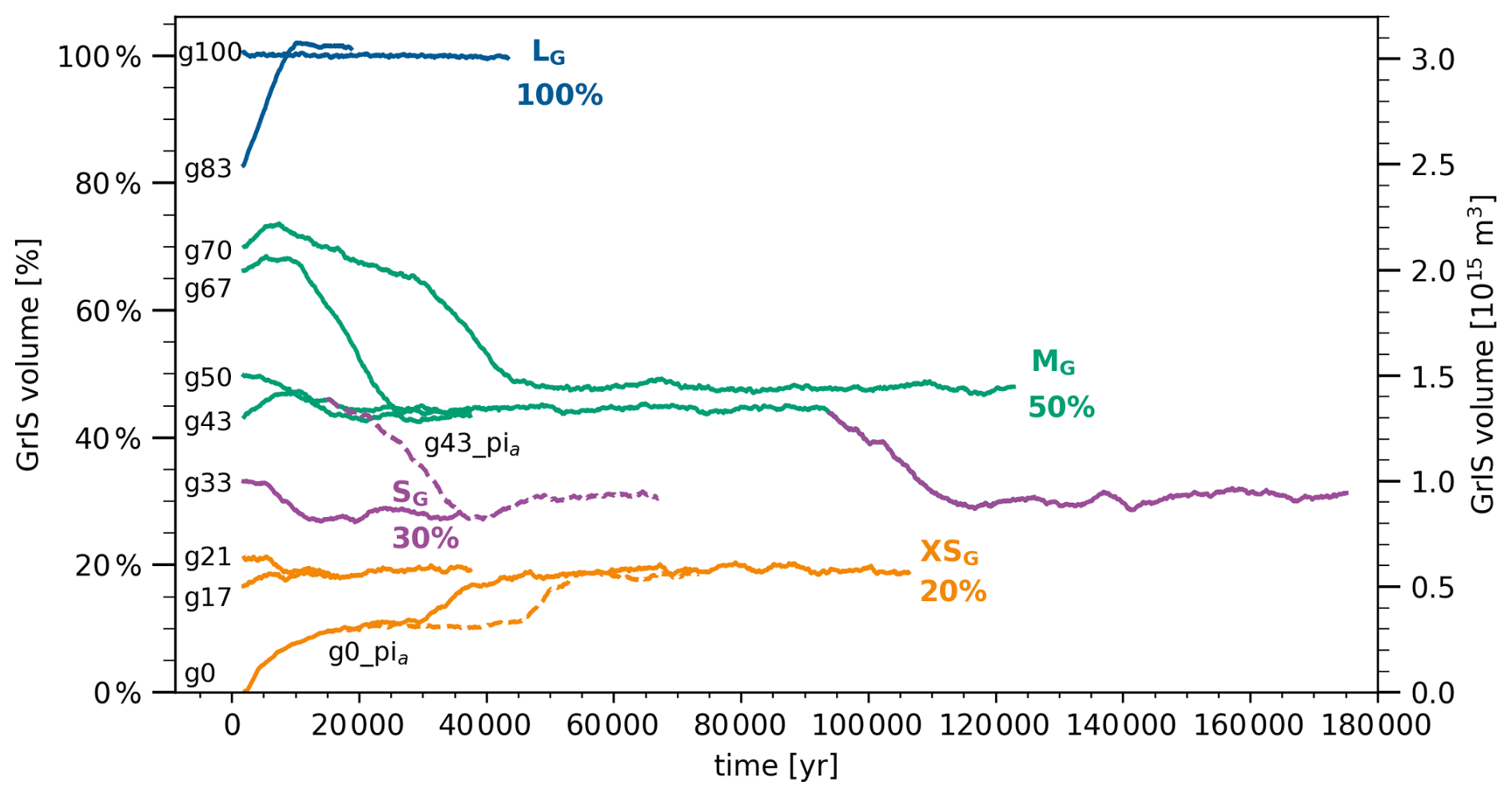
Figure 2 Time series of the GrIS equilibrium simulations and their final steady states given as end volume with respect to the PI volume in percent. Solid lines indicate the steady-state simulations performed with interactive ice sheets in the Northern and Southern Hemisphere. Dashed lines show the same experiments but performed with a prescribed PI AIS from g100. Each color corresponds to one steady state. The change in the color of g43 indicates a state transition that is further explained throughout the text. The simulations used to study the climate conditions constraining each state displayed in Fig. 1 are highlighted with the steady state's name and equilibrium volume. Maps of the initial GrIS and AIS volumes are illustrated in Figs. A1 and A2 in the Appendix.

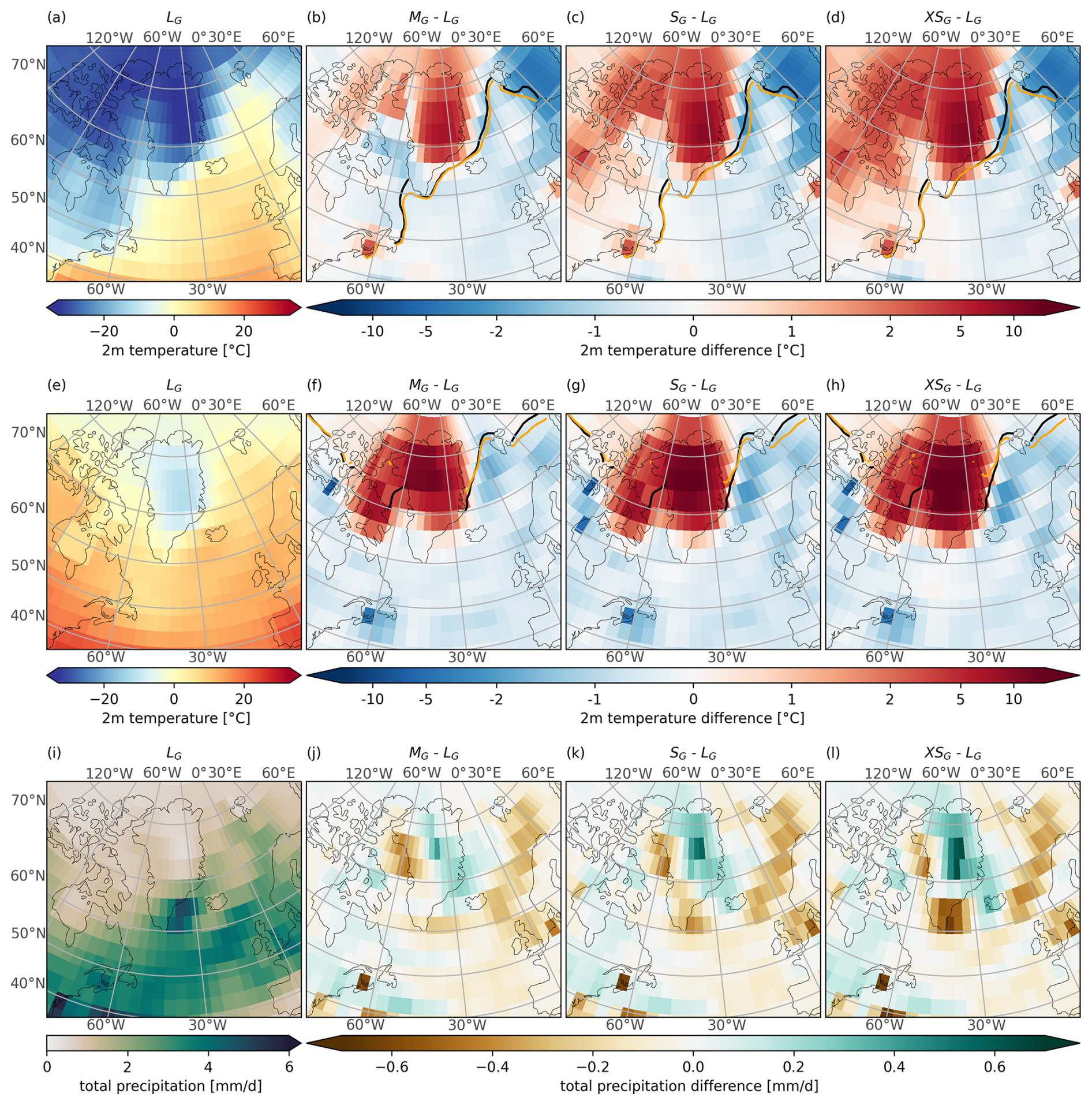
Figure 3 2 m air-temperature in (a–d) DJF and (e–h) JJA as well as (i–l) annual-mean total precipitation. The first column shows L_G, the remaining columns show the anomalies of M_G, S_G and XS_G relative to L_G. (b–d) and (f–h) and also display the winter and summer sea-ice margin of each experiment. L_G is shown in black and M_G, S_G and XS_G in orange. Note the logarithmic colorbar in (b)–(d) and (f)–(h).

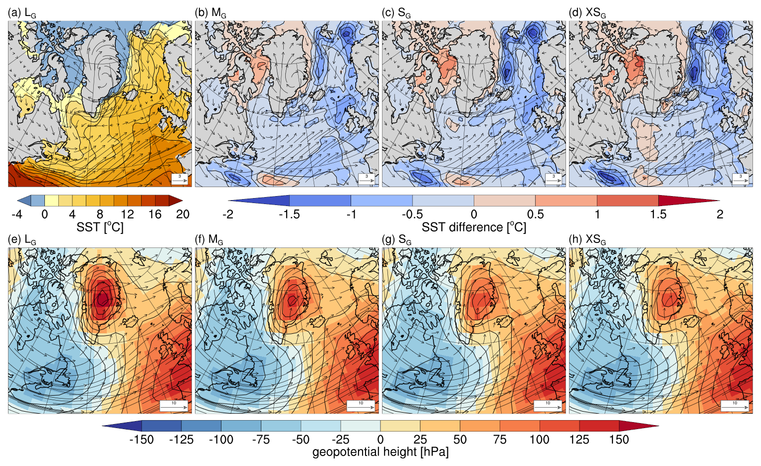
Figure 4 (a–d) Absolute annual mean 10 m winds (vectors, m s⁻¹) overlaid on SST. (a) shows absolute SST from L_G, (b–d) the difference in SST between M_G, S_G and XS_G with L_G, respectively. (e–h) DJF normalized geopotential height (contours) and flow direction (vectors, m s⁻¹) at 500 hPa.

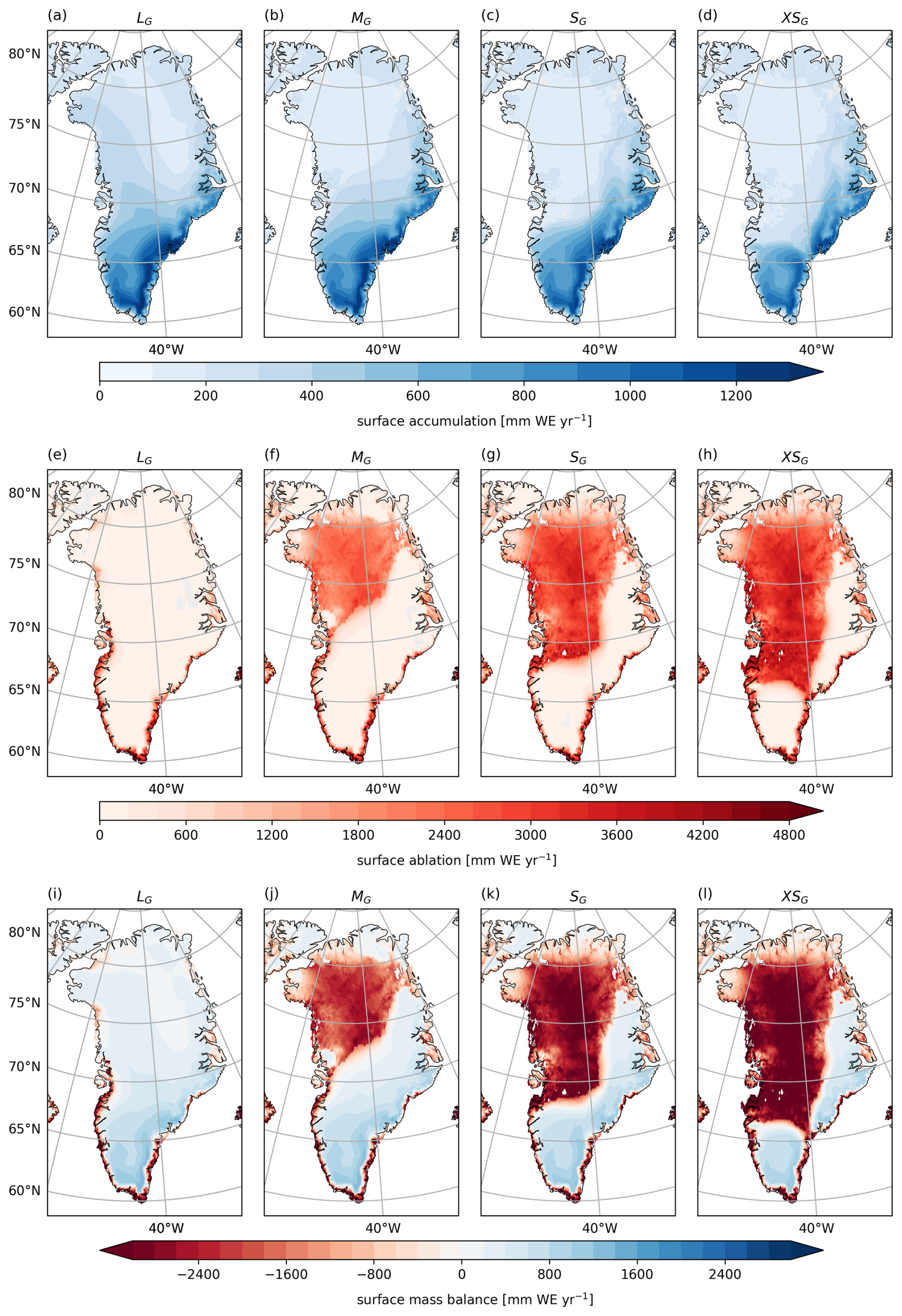
Figure 5 Surface accumulation (top row), surface ablation (middle row) and SMB (bottom row) for the four steady states L_G, M_G, S_G, XS_G and (from left to right). Results are derived by interpolating the annual three-dimensional SMB output of MPI-ESM/mPISM/VILMA, averaged over the last ESM 1000 years, onto the topography of each steady state.

Started from a completely disintegrated state (Appendix Fig. A1a), the GrIS regrows in the regions in the south and east of Greenland (XS_G) due to their favorable climatic conditions, including temperature and precipitation. The east of Greenland receives more precipitation than with a large GrIS as the atmospheric flow is less deflected by the lower orography of the smaller GrIS (Fig. 3l). As a consequence, moist air masses and storm tracks penetrate deeper into Greenland (previously shown by Andernach et al., 2025), where they eventually precipitate on the windward side of the mountain range to the east of Greenland. This is reflected in a more homogeneous distribution of precipitation, with lower precipitation in the south and west of Greenland, but higher precipitation in the northeast in XS_G. The weaker Greenland Anticyclone (previously shown by Andernach et al., 2025), in response to the reduced mechanical blocking and the higher near-surface air temperatures in the predominantly low-elevation areas of Greenland (Fig. 3d and h), further reduces the advection of moist air masses to southern Greenland. Hence, surface accumulation is lower in Greenland's south and west in XS_G than in L_G (Fig. 5d). Nevertheless, the southern and eastern regions continue to receive the highest annual precipitation, due to orographic effects and the proximity to the core of the storm track located south of Greenland. Only in the mountains are temperatures cold enough to preserve the snow throughout the year (Fig. 5h and l), which eventually favors the nucleation of a new ice sheet.

The differences in the climate of XS_G compared to S_G also inhibit ice sheet expansion into the center and north of Greenland. In the center and the north, a strong lapse-rate effect due to the lower surface elevation of up to 2300 m (XS_G compared to L_G) inhibits ice sheet formation by raising temperatures. Assuming a lapse rate as used in our EBM, we find a temperature increase of up to 10.6 °C in the areas of the largest change in surface elevation. Thus, the lapse-rate effect contributes most strongly to the annual-mean temperature change of up to 11.7 °C in XS_G as compared to L_G. This lapse-rate effect also explains why the highest temperature anomaly occurs in central and northern Greenland (Fig. 3d). Although the warming effect of the lower surface elevation due to the lower ice thickness of the smaller GrIS is slightly counteracted by GIA effects, which raises the bedrock surface by up to 600 m over central Greenland (Fig. 6d), cooling through GIA is not sufficient to allow for an expansion of the GrIS in XS_G. Another contribution arises from the smaller glacier mask and the absence of a snow cover in summer, which changes surface parameters to those of a non-glaciated surface. The latter enables the dynamic growth of grass and shrubs in ice-free areas. These surface changes reduce the summer albedo by about 0.6, leading to a strongly positive melt–albedo feedback. They also allow surface temperatures to exceed the melting point in XS_G. Owing to this surface-property effect, the warming relative to a large GrIS is stronger in summer (up to +17.0 °C) than in winter (up to +11 °C). Hence, no perennial snow cover can accumulate north of the northwestern margin of the GrIS in XS_G, although precipitation is larger with a smaller GrIS in these areas (Fig. 3i–l).

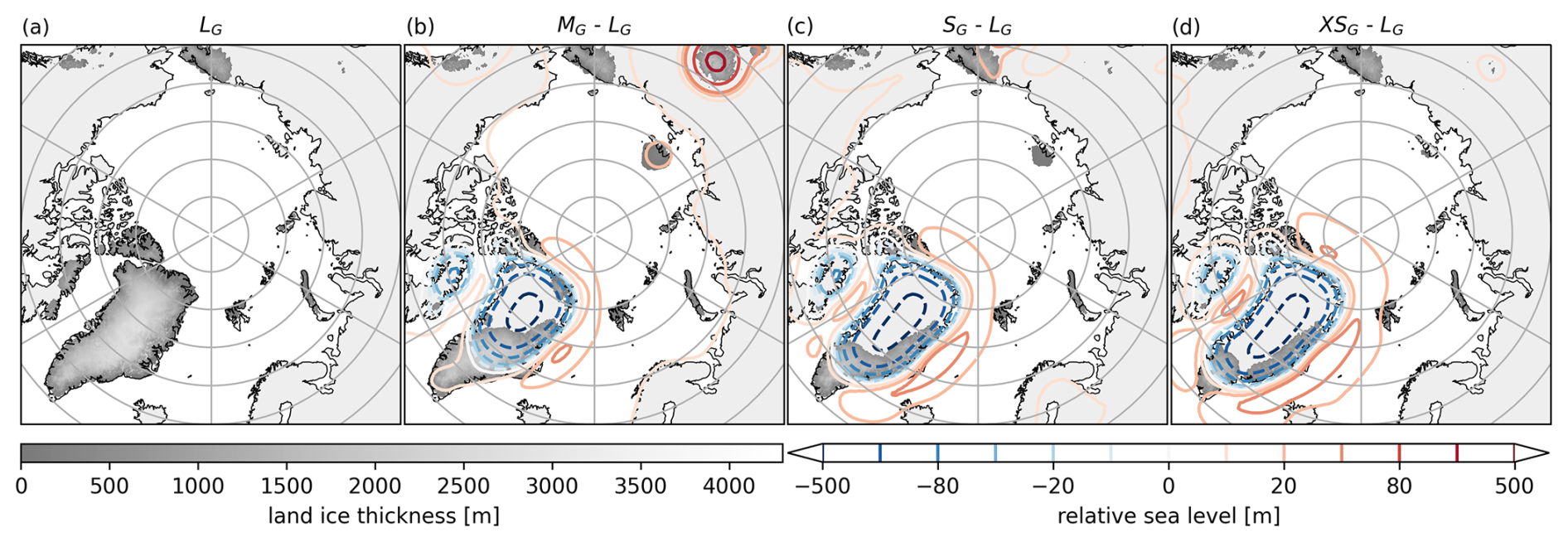
Figure 6 Effect of glacial isostatic adjustment (GIA), shown as the relative sea level, and ice sheet thickness for each steady state. The left column displays the absolute values of L_G. The remaining columns show the difference in relative sea level of each state compared to L_G, depicted as colored contour lines, ranging from lower sea levels (blue) to higher sea levels (red). Gray filled contours show the ice-sheet thickness of each state.

Another warming contribution in XS_G arises from the near-surface winds that approach Greenland on its southeast coast (Fig. 4a–d). Traversing Greenland, winds are forced to ascend over the very small GrIS and create a slight Föhn effect on the leeward side. This is expressed in warmer temperatures, a strong reduction in precipitation and down-slope winds on the leeward side as compared to the windward side of the ice sheet. This Föhn effect contributes to preventing an ice sheet expansion into the central, western and northern areas of Greenland as well as the connection of the eastern and the southern parts of the very small GrIS.

The smaller GrIS in XS_G is also stabilized by differences in the atmospheric circulation. In response to the reduced blocking effect of a smaller GrIS, the quasi-static wave at 500 hPa over Greenland is slightly shifted eastward and weaker (Fig. 4h). This shift reinforces the meridional flow pattern over Greenland and its surroundings, similar to findings of Andernach et al. (2025). Consequently, the southerly wind component over Greenland intensifies, advecting more warm air masses towards Greenland. This enhances the 2 m air-temperature rise over Greenland and contributes to preventing the expansion of the very small GrIS in XS_G. Over the adjacent Nordic Seas, the wind direction is increasingly northerly, amplifying the influx of cold polar air, as visible by colder 2 m air-temperatures over the Nordic Seas and Scandinavia (Fig. 3d and h). Additionally, the northerly winds drive sea ice further south and favor sea-ice expansion in the Nordic Seas particularly in winter (Fig. 3d). The larger sea-ice cover in XS_G reduces heat loss from the ocean to the atmosphere, enhancing the cooling of the overlying atmosphere. This also leads to colder upper ocean temperatures until a depth of approximately 150 m and warmer temperatures at deeper levels. A weaker AMOC strength at 30° N in XS_G (14.6 Sv) compared to L_G (17.3 Sv) further reduces the heat that is transported northwards, contributing to the colder upper ocean temperatures in the Nordic Seas. As the colder air is advected onto the GrIS by the southeasterly near-surface winds (Fig. 4d), this cold ocean anomaly likely contributes to preserving the southern part of the very small ice sheet in XS_G. Analyzing the variability of the AMOC and the SMB in XS_G, we find a linear relationship with an increase in SMB by 40.7 mm water equivalent (w.e.) per 1 Sv decrease of the AMOC strength.

To explore the importance of the ocean cooling in the Nordic Seas for the stability of the GrIS in XS_G, we conducted a sensitivity experiment. In this experiment, we used the same setup as in g0, where the GrIS stabilizes at XS_G, but with SST and SSS nudged towards the climatology of g100, which corresponds to the PI state. Hereafter, this experiment is referred to as g0_pi_oce (Table 1). Hence, this experiment only considers interaction of the ice sheets with the atmosphere and sea ice, while suppressing feedback with the ocean. In the absence of the ocean cooling in the Nordic Seas (g0_pi_oce), a new ice sheet develops only in the east of Greenland, while no regrowth occurs in the south of Greenland. Hence, the cooling of the Nordic Seas, caused by an absent or much smaller GrIS, is a necessary prerequisite for the development of an ice sheet in Greenland's south and feedbacks with the ocean maintain the southern GrIS.

Above an initial volume of 21 %–33 % of its PI volume (0.6–1.0 × 10¹⁵ m³), the GrIS transitions into the next larger state, S_G. The GrIS in S_G as well as M_G is stabilized by similar climate conditions and feedbacks, as described for XS_G (Figs. 3 and 4). However, being strongly controlled by orography and ice sheet area, the atmospheric circulation signals are weaker when the GrIS is larger.

In S_G, the ice ridge between the eastern and the southern GrIS originates from a colder climate. The ice ridge increases the surface elevation and albedo, and also keeps surface properties in a glaciated state, leading to colder temperatures than in XS_G (i.e., elevation and albedo feedback; Fig. 3c and g). Due to orographic effects, accumulation is higher on the windward side and atop of the ice ridge compared to XS_G (Fig. 5c). The lower ablation and higher accumulation stabilize the connection between the eastern and the southern part of the GrIS. On the leeward side of the ice ridge, however, a Föhn effect inhibits an ice sheet expansion towards the northwest in S_G. S_G only has a small range of stability. Above a threshold of 33 %–43 % of its PI volume (1.0–1.3 × 10¹⁵ m³), the GrIS becomes unstable and transitions into M_G, due to the effects of the higher surface elevation, the larger glacier mask, a weakening of the southerly winds, weaker Föhn winds, a less strongly redistributed precipitation and more ice flowing into the central areas.

M_G can be attained from a relatively large range of initial values (Fig. 2). However, it is less stable than the other states. This is evident in the simulation g43, which is a stable M_G state for more than 80 000 years before it abruptly transitions into the next smaller state S_G. The state transition coincides with a slightly stronger AMOC, whose increase is within the bounds of natural variability (e.g.,  Latif et al., 2022; Ferster et al., 2025). In the first 1000 ice sheet years of the transition, the AMOC is stronger by on average 1.3 Sv compared to the preceding millennia. The stronger AMOC transports more heat northward into the North Atlantic Ocean, where it leads to a warm anomaly in the Irminger Sea and the Nordic Seas. This warm anomaly is advected onto the GrIS by southeasterly winds off the southeast coast of Greenland (Fig. 4b). Over the GrIS, the warmer air triggers melting of the northwestern part of the ice sheet. Together with the climate–ice sheet feedbacks described, the medium GrIS in g43 enters self-sustained melting and transitions into S_G. In contrast, the medium GrIS in the simulation initiated with 70 % of the GrIS volume (g70) remains stable throughout our simulated time period. As both simulations have a similar and stable ice volume and ice distribution for about 80 000 years, we consider g43 before the transition also as M_G state. However, subjected to small disturbances, the M_G initiated from 43 % of GrIS volume eventually destabilizes and transitions into a more stable equilibrium state. Hence, we consider the final part of g43 as S_G state.

Similar to the smaller states XS_G and S_G, an expansion of the GrIS in M_G is impeded by a strong lapse-rate effect, the absence of glacial surface conditions in the northwest, and to a lesser degree by a slightly different atmospheric circulation and a redistribution of precipitation, which cause a negative SMB in central and northwest Greenland (Figs. 3b, f, j and 5j). Resting primarily on low-elevation and flat bedrock, the northwestern part of the GrIS is exposed to warmer temperatures and lacks stabilizing pinning points over high-elevation terrain (Fig. 1b), controlling ice sheet growth in this region. Hence, even started from a significantly larger GrIS volume of 70 % with the ice edge further in the northwest (Fig. A1h), the GrIS returns to M_G (Fig. 2). Only above a threshold of 70 %–83 % of its PI volume (2.1–2.5 × 10¹⁵ m³), does an ice cover in the northwest become stable, as it connects with the northern part of the GrIS and transitions into L_G (Fig. 2). Hence, there is no stable state with an ice cover in the flat and low-lying northwest that is not connected to the northern part of the GrIS. This explains the absence of a stable state between 50 % and 100 % of its PI volume.

3.3 Contributions of the individual climate–ice sheet feedbacks

But how important is each of these described feedbacks and processes for the stability of the GrIS states? Figure 7 summarizes the contribution of each feedback, based on the figures in Appendix B. The figure indicates, for instance, that the GrIS in S_G is stable mostly due to the impact of the surface elevation feedback. As explained in Sect. 2.2, the surface elevation effect is composed of the effect of the ice thickness and the counteractive GIA. In S_G, the surface elevation is significantly lower over large parts of Greenland than in M_G, due to the smaller ice sheet and associated lower ice thickness. Although uplift through GIA counteracts the effect of the lower ice thickness, the net impact of these two feedbacks is destabilizing, as the ice thickness-induced elevation change is larger than the isostatic uplifting-induced elevation change. The combined glacier mask and surface albedo feedback further impedes an ice sheet expansion along the margins of the GrIS in S_G, mainly by raising the surface ablation. On the other hand, the higher surface elevation and larger glacier mask than in XS_G stabilize the GrIS in S_G. Feedback with the precipitation opposes the elevation and glacier mask feedback mainly due a redistribution in the accumulation, similar to Fig. 3j–l. While the precipitation of S_G favors ice-sheet expansion towards the north of Greenland, thus stabilizing the small GrIS, the redistribution reduces the SMB in the south of Greenland. For the transition from a small to a very small GrIS (S_G→XS_G), the redistribution of precipitation has a counteracting effect and destabilizes the GrIS in S_G. The ocean feedback has the weakest impact on the stability of the small GrIS in S_G. Warmer ocean conditions in the Baffin Bay and Irminger Sea compared to colder conditions in the Nordic Seas in S_G than in M_G (Fig. B1j) favor ice sheet growth in the west, but inhibit it in the east. Spatially averaged, feedback with the ocean thus contributes to impeding the shift of the small GrIS into the medium state. However, the ocean changes slightly contribute to preventing a retreat of the GrIS in S_G, due to a cooling-related lower surface ablation in S_G than in XS_G (Fig. B2j). Although the ocean feedback has a smaller or even minor contribution compared to the elevation feedback, even these small contributions can be decisive for critical transitions of the ice sheet, as explained in the preceding analysis, and should therefore be included in analyses of the stability of the GrIS.

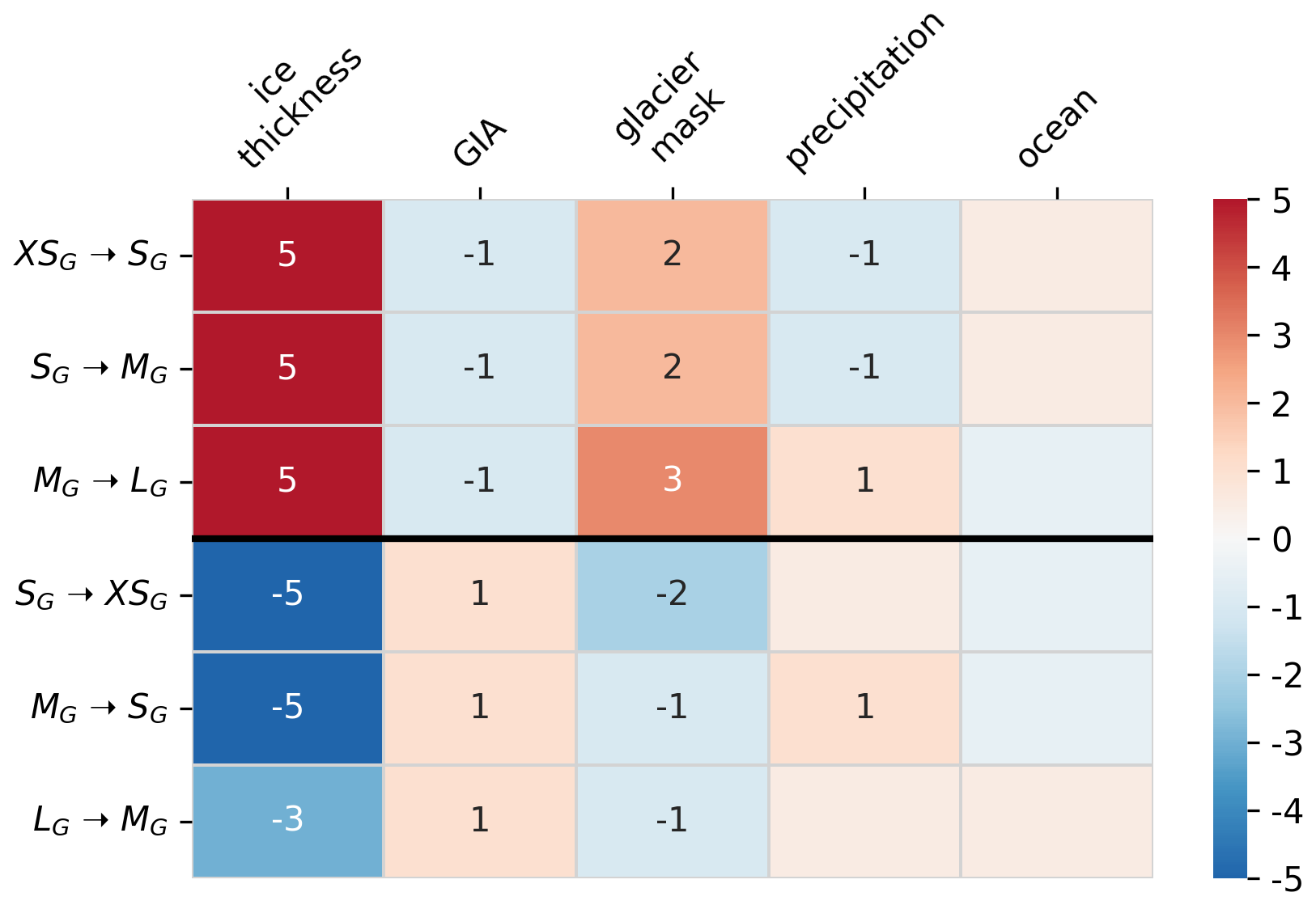
Figure 7 Contribution of the different feedbacks and processes between the GrIS and the climate system to stabilizing the steady states. The number and associated color indicate the magnitude of the contribution of the respective factor to stabilizing (negative number and blue) or destabilizing (positive number and red) a GrIS state. It is calculated as the spatially-averaged difference between the SMB field of each steady state and the SMB field of this state including the indicated feedback based on its neighboring GrIS state in Appendix B (e.g., SMB of XS_G minus the SMB calculated under the climate of XS_G but with the precipitation scaled to the precipitation field of S_G). The spatial averages are computed for the non-overlapping area between the two different glacier masks in central Greenland (solid and dashed lines in Appendix Figs. B1 and B2), excluding scattered coastal grid cells. Boxes without numbers indicate that the contribution is small. The upper half of the table shows the contributions for a transition from a smaller into a larger GrIS state and the bottom half of the table for a transition from a larger into a smaller GrIS state. The intervals used for scaling are: 0–50 $\mathrm{mm}\mathrm{w}.\mathrm{e}.{\mathrm{yr}}^{-\mathrm{1}}$ (boxes without numbers), 51–500 $\mathrm{mm}\mathrm{w}.\mathrm{e}.{\mathrm{yr}}^{-\mathrm{1}}$ (−1), 501–1000 $\mathrm{mm}\mathrm{w}.\mathrm{e}.{\mathrm{yr}}^{-\mathrm{1}}$ (−2), 1001–1500 $\mathrm{mm}\mathrm{w}.\mathrm{e}.{\mathrm{yr}}^{-\mathrm{1}}$ (−3), 1501–2000 $\mathrm{mm}\mathrm{w}.\mathrm{e}.{\mathrm{yr}}^{-\mathrm{1}}$ (−4) and > 2000 $\mathrm{mm}\mathrm{w}.\mathrm{e}.{\mathrm{yr}}^{-\mathrm{1}}$ (−5) for negative feedbacks and mirrored for positive feedbacks. Note that glacier mask also includes the albedo feedback.

The contributions to the stability of the other states are mostly comparable. An exception is the positive precipitation contribution for the transition of a medium to a large GrIS (M_G→L_G) as compared to the negative precipitation contribution for the transitions of a very small and a small GrIS to the next larger state (XS_G→S_G and S_G→M_G). It is attributed to the precipitation-induced higher surface ablation with a medium than with a large GrIS, as higher summer rainfall and lower summer snowfall increase the energy available for surface melt. Thus precipitation has a stabilizing effect on the M_G state, limiting further GrIS regrowth.

3.4 Interlinked stability of the GrIS and AIS states

By including interactive ice sheets in both hemispheres, the model setup allows for changes in both the GrIS and the AIS volumes. Here we discuss how changes in the GrIS's geometry impact the AIS and vice versa.

3.4.1 Impact of GrIS changes on the stability of the AIS

We find that changes in the GrIS volume impact the stability of the AIS. In g0, which stabilizes at XS_G, we initially removed the GrIS and let it regrow under PI climate conditions. 12 500 years after the initialization of the experiment, the AIS starts to lose mass. Within approximately 46 000 years, 18 % of the total AIS volume disintegrates, corresponding to about 0.5 × 10¹⁶ m³ or 6.7 m SLE. A potential trigger of this mass loss is a change in the global sea-level (Wunderling et al., 2021), which promptly rises by more than 7 m due to the removal of the GrIS. Particularly the West Antarctic Ice Sheet (WAIS) is highly vulnerable to such a sea-level rise, due to its extensive marine-based sectors that are located on low-lying land and are in direct contact with the ocean. Previous studies found that a local increase in sea level can lead to a grounding line retreat (Denton and Hughes, 1983; Denton et al., 1986; Schoof, 2007; Gomez et al., 2020), by increasing the ice flux at the grounding line, turning grounded ice into floating ice (Schoof, 2007). A thinning and retreat of the floating ice, for example through subsurface melting, can reduce the buttressing effect of the WAIS ice shelf on inland ice, which can flow faster, as previously described (e.g., Joughin and Alley, 2011). Hence, the mass loss of the AIS can be mainly attributed to a collapse of the WAIS, which decreases to about 20 % of its original volume in g0. In contrast, the East Antarctic Ice Sheet (EAIS) consists primarily of grounded ice that is isolated from the ocean, which renders it less sensitive to changes in sea level. The destabilized and retreated grounded ice of large parts of Marie Byrd Land and Ellsworth Land (Fig. 8e) allows to open up new ocean passages that connect the Weddell Sea with the Amundsen and Bellingshausen Seas as well as the Amundsen Sea with the Ross Sea beneath the ice shelf in g0.

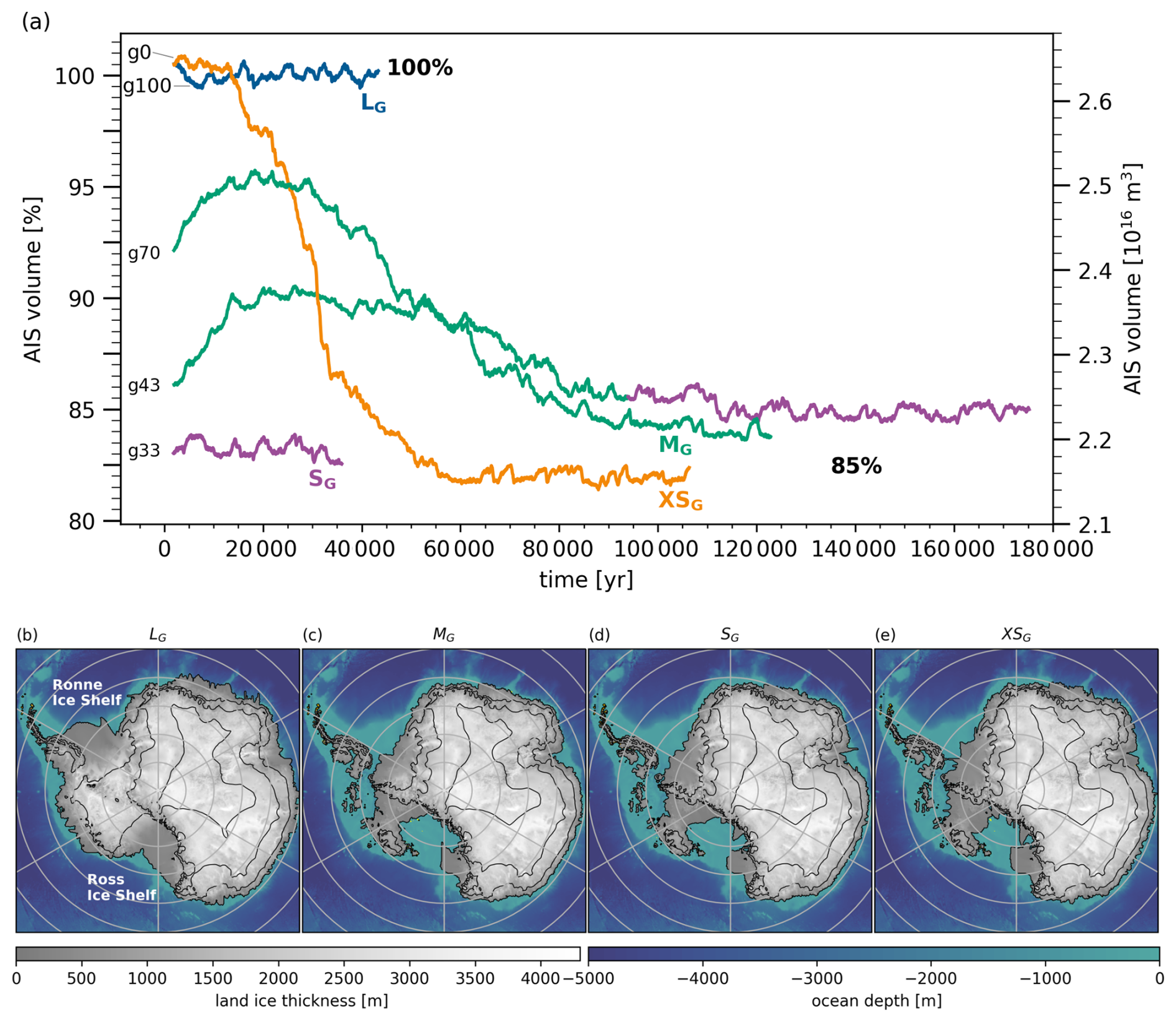
Figure 8 (a) Time series of ice volume of the AIS in the simulations selected to study the climate conditions of the GrIS's steady states in Sect. 3.1 and in simulation g43. The colors correspond to the colors of the GrIS's steady state in Fig. 2. The change in the color of g43 indicates when the GrIS transitions from M_G into S_G. (b–e) Maps of ice thickness of the AIS in the selected GrIS steady-state simulations. Maps of the initial AIS volumes are illustrated in Fig. A2 in the Appendix.

g33, g43 and g70, with their final GrIS states of S_G and M_G, were branched off from a simulation with regrowing ice sheets under declining CO₂ concentrations (Sect. 2.2). At the time when g33 was branched off, the AIS had not yet started to regrow as temperatures were still too warm. Hence, its initial volume is similar to the final AIS volume of g0 (Fig. 8c and d). g43 and g70 have been branched off at a time when the AIS had started to regrow. The initial increase in ice volume of the AIS in these simulations arises from the slow response time of the ice sheet due to which the AIS needs several millennia to adjust to the new climate conditions. As g70 was branched off later than g43, its initial volume of the AIS is larger. In all three simulations, g33, g43 and g70, the AIS stabilizes at a similar final volume as g0 with approximately 85 % of its PI volume, equivalent to a mass loss of about 5.5 m SLE.

3.4.2 Significance of AIS interactions for GrIS stability

As discussed in the previous section, changes in the GrIS affect the AIS geometry. To investigate if and how the AIS volume also impacts the steady states of the GrIS and to estimate the error introduced by omitting AIS dynamics in studies of the stability of the GrIS, we designed two simulations with a prescribed constant PI AIS (g0_pi_a and g43_pi_a; Table 1). In these simulations only the GrIS is interactive. This allows us to estimate the direct effect of an interactive AIS on the GrIS's steady states. In the following, we compare these experiments to the fully interactive experiments (g0 and g43, respectively).

The final XS_G and S_G state of g0 and g43, respectively, appear to be insensitive to the changes in the AIS (Fig. 2), but the timing of transitions during the stabilization of the states changes. The rapid increase in volume around year 30 000 from a much smaller GrIS volume into the final XS_G state in g0 is delayed in response to altered AIS dynamics in g0_pi_a. The processes that lead to the rapid transition have been analyzed through additional sensitivity experiments and are detailed in Appendix C. They suggest that this transition is determined by the dynamics of the ice sheet. With a small, yet steady, growth rate in southern Greenland, a rapid increase into the final XS_G state takes place as individual glaciated grid points connect in g0. The disturbance of imposing a PI AIS in g0_pi_a leads to a different timing of regrowth in southern Greenland. We find that this delay is caused by a 1.1 Sv stronger AMOC with a constant PI AIS as compared to a smaller AIS (g0_pi_a compared to g0 in Fig. 9a). The stronger AMOC enhances heat transport to the North Atlantic Ocean. This leads to a warm anomaly in the Irminger Sea and the Nordic Seas and warmer near-surface air being advected onto the GrIS by the southeasterly winds off the southeast coast of Greenland (Fig. 4d), as the atmospheric circulation in and around Greenland remains unaffected by the change in the AIS volume. The warm air advection impedes the regrowth of ice in the south of Greenland. However, the warm air advection subsides as the simulation g0_pi_a progresses and eventually allows for the regrowth of ice in southern Greenland and the transition into the same final state as with the interactive smaller AIS in g0. This rapid transition after year 40 000 in g0_pi_a (Fig. 2) coincides with a weaker AMOC. During years 40 000 to 45 000, the AMOC is weaker by on average 1.4 Sv compared to the years before 40 000 (Fig. 9a). We relate the AMOC weakening to natural variability, which can occur on centennial to millennial timescales.

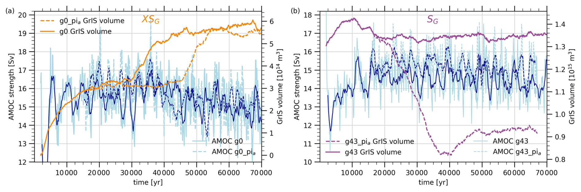
Figure 9 AMOC strength and GrIS volume during GrIS state transitions in simulations with an interactive AIS (solid lines) and a constant PI AIS (dashed lines). (a) shows the effect of AIS dynamics on the simulation g0, which is stable at XS_G, and (b) on the simulation g43, which eventually stabilizes at S_G. Note that the ice volume is plotted as 10 year means, whereas the AMOC is plotted as 100 year means due to the asynchronous coupling method. The dark blue lines show the AMOC smoothed with a moving window of n=10.

Similarly, M_G in g43_pi_a loses stability and transitions into S_G shortly after the disturbance of imposing a PI AIS. Comparable to the transition from M_G to S_G simulated around the year 90 000 in g43 (Sect. 3.2), the mass loss in g43_pi_a coincides with a slightly stronger AMOC (+0.9 Sv) in response to the constant PI AIS compared to a smaller AIS in g43 (Fig. 9b). Over the GrIS, the warmer near-surface air advected from the ocean triggers melting of the northwestern part of the ice sheet. In combination with the climate–ice sheet feedbacks described in Sect. 3.2, the medium GrIS enters self-amplified melting with a constant PI AIS in g43_pi_a and transitions into S_G earlier than with a smaller AIS in g43.

4 Discussion

In this study we investigated the steady states of the GrIS under PI CO₂ concentrations with a comprehensive ESM that accounts for interactive ice sheets in both hemispheres. We find that the GrIS is multistable, exhibiting at least four steady states under PI CO₂ concentrations. This confirms previous modeling studies that found more than one steady state of the GrIS in a PI, PD or a slightly warmer climate using numerical models or other approaches that did not capture all important feedback mechanisms between the ice sheets and the climate system (Crowley and Baum, 1995; Toniazzo et al., 2004; Vizcaíno et al., 2008; Ridley et al., 2010; Langen et al., 2012; Robinson et al., 2012; Solgaard and Langen, 2012; Gregory et al., 2020; Höning et al., 2023). The existence of several steady states means that if disintegrated under higher CO₂ concentrations, the GrIS cannot return to its PI volume even if CO₂ concentrations are lowered to PI values. Once reduced below a volume threshold of about 83 %–70 %, equivalent to a loss of 1.2–2.1 m SLE, parts of the ice sheet are lost irreversibly in our simulations and the GrIS stabilizes at the M_G state with 50 % of its PI volume. Due to the absence of ice in central Greenland, the volume of M_G is smaller than of the largest medium states found in previous studies (approximately 80 % and 60 % in Ridley et al., 2010 and Gregory et al., 2020). This irreversibility threshold is only slightly lower than the threshold of 90 %–80 % that has been suggested by Ridley et al. (2010), but higher than the threshold of 4 m SLE suggested by Gregory et al. (2020). Below 43 %–33 %, even further parts of the GrIS are lost irreversibly and the GrIS enters a small state with 30 % of its PI volume. Hence, we show a second intermediate state that is smaller than the intermediate states found in Gregory et al. (2020). Below the volume threshold of 33 %–21 %, the GrIS stabilizes at XS_G with 20 % of its PI volume. The volume of our smallest state resembles that of Ridley et al. (2010) under PI conditions and of Robinson et al. (2012) under a summer temperature anomaly of 1 °C, but is less than half of the size of the one from Gregory et al. (2020). This indicates that long-term sea-level rise after a disappearance of the GrIS could be much higher than previously suggested. In our simulations, the GrIS contributes to between 3.7 m SLE (M_G) and 5.9 m SLE (XS_G). As diverging temperature thresholds for the full recovery of the GrIS have been found (Letréguilly et al., 1991; Robinson et al., 2012; Solgaard and Langen, 2012; Höning et al., 2023), the reversibility should be investigated further with other coupled ISM-ESMs, that offer a comprehensive representation of the physical processes and feedbacks between ice sheets and the climate system.

Slow regrowth over tens of millennia begins in the eastern mountains of Greenland, followed by the southern mountains in our simulations. This is in line with previous work (Letréguilly et al., 1991; Ridley et al., 2010). Due to orographic effects these high elevation areas provide favorable conditions for snow to accumulate and are cold enough to form a perennial snow cover. The northeast shift in precipitation, due to the reduced blocking in response to a disintegration of the GrIS (see also Solgaard and Langen, 2012 and Andernach et al., 2025), further supports accumulation in the east. Once the SST in the Irminger Sea and the Nordic Seas has cooled sufficiently in response to the stronger northerly wind direction and the sea-ice feedback, regrowth continues in the mountains of southern Greenland. However, the recovery remains incomplete, controlled by the climate changes in response to an absent or significantly smaller GrIS.

The simulated climate response to an absent or much smaller GrIS is similar to the response obtained with stand-alone MPI-ESM simulations without the GrIS under PI climate conditions (Andernach et al., 2025). Yet, including climate–ice sheet feedbacks, we find that the melt–elevation feedback is the dominant process that prevents a complete recovery, similar to Petrini et al. (2025). Its contribution is enhanced by the melt–albedo feedback and effects associated with the glacier mask, previously highlighted by Zeitz et al. (2021). Although interactions with the precipitation pattern, the atmospheric circulation and ocean dynamics contribute less to the stabilization of the steady states, we argue that they should not be neglected in studies of the stability of the GrIS. Especially when the ice sheet is close to a critical transition, a small perturbation is sufficient to trigger a state transition. A northwestward expansion of the smaller GrIS states is further constrained by the absence of topographic pinning points, which could serve as seeding points for ice sheet regrowth over the flat terrain and in in the lee of the GrIS, as suggested by Petrini et al. (2025). The location in the lee makes the smaller states particularly susceptible to Föhn winds. Langen et al. (2012) showed that this effect effectively hinders the regrowth in a coupled model. The northwestern part of the GrIS is also absent in smaller states found previously (Ridley et al., 2010; Gregory et al., 2020). The absence of a stable solution with an ice sheet in the northwest unconnected to the northern part of the GrIS explains the absence of a stable state between 50 % and 100 %.

An example of the importance of sea-surface effects is the stability of the southern part of the GrIS. It is significantly controlled by the SST and the sea-ice cover of the surrounding ocean. In our simulations, the cooling of the Nordic Seas and of parts of the Irminger Sea and Iceland Basin in absence of the large GrIS (Fig. 4b–d) drives the regrowth of ice in southern Greenland. Without the cooling signal of the ocean, this region would not have regrown into XS_G started from an ice-free Greenland (Sect. 3.2). This highlights the importance of using a fully-coupled model to examine the steady states of the GrIS. Different degrees of model complexities might explain why the presence of an ice sheet in the south of Greenland in regrown states varies between studies, whereas regrowth in the east is a robust feature across different models (Letréguilly et al., 1991; Lunt et al., 2004; Ridley et al., 2010; Langen et al., 2012; Solgaard and Langen, 2012; Gregory et al., 2020). The absence of the full range of ocean-atmosphere interactions in an AGCM study by Gregory et al. (2020) might account for the missing southern part in several of their regrown states. Additionally, their coarse horizontal grid spacing of 7.5° longitude by 5° latitude likely cannot resolve regional topographic peaks. As a consequence, their model may underestimate the extent to which the southern region provides favorable conditions for ice sheet regrowth. The build-up of ice in southern Greenland also depends on the interpolation method applied to temperature and precipitation as found by Solgaard and Langen (2012). This underpins the sensitivity of ice sheet regrowth in the south of Greenland to various factors, such as model resolution and the integration of feedback processes.

Similarly, the inclusion of various additional feedback mechanisms, such as meltwater release of icebergs and changes in the land–sea mask, may account for differences in the ice volume in our study compared to previous research. For example, an interactive land–sea mask is crucial for accurately representing changes in ocean-mass transport through Arctic gateways in response to changes in the GrIS and AIS volume and the associated sea-level rise (Andernach et al., 2025). Dynamics in the geometries of the straits – including their opening, closing, and geometric changes – impact the volume and patterns of water, sea ice, salt and heat transport, all of which impact the climate over the ice sheets. Another important feature of our model setup is the dynamic integration of both ice sheets, the AIS and GrIS, which is in contrast to previous modeling studies of the stability of the GrIS using a prescribed PI AIS (Ridley et al., 2010; Langen et al., 2012; Robinson et al., 2012; Solgaard and Langen, 2012; Gregory et al., 2020; Höning et al., 2023). Although the dynamics of the AIS do not impact the final steady states, they can impact the timing of state transitions during their stabilization through impacts on the AMOC. It is also possible that the final M_G state in g70 has a similarly low stability as the initial M_G state in g43 and could destabilize with a prescribed PI AIS. Note that our asynchronous coupling between the climate model and the ISM might influence the exact timing of the transitions in the ice sheet states. However, with temporal offsets in the GrIS transitions exceeding 10 000 years depending on AIS dynamics, our findings are robust against the uncertainty introduced by the coupling technique.

Lastly, our study indicates that it is necessary to run simulations of the stability of GrIS over tens of thousands of years to achieve equilibrium due to the long time scales inherent to the ice sheet's dynamics. Further, in a coupled set-up, the deep ocean needs millennia to equilibrate after a disturbance. As changes in the deep ocean can alter the distribution of heat, salinity and density, this can also affect the atmospheric circulation. Changes in the atmosphere can in turn influence temperature and precipitation patterns over Greenland, impacting the ice sheet's SMB. Particularly when the ice sheet is close to a critical transition or only weakly stable, it requires only a minor perturbation to shift states. We show that even small variations in the AMOC can trigger significant and abrupt changes in the GrIS. These AMOC variations can be caused, for example, by natural climate variability (Latif et al., 2022; Ferster et al., 2025), as in g43, or by volume changes of the AIS, as shown in our constant AIS experiments. Earlier studies suggested that freshwater input from the AIS has an impact on deep convection around Antarctica and the AMOC due to processes linked to the bipolar seesaw (Mikolajewicz, 1998; He and Clark, 2022; Sinet et al., 2023). This means that also M_G in g70, despite its apparently greater stability due to its slightly higher volume and larger ice cover in the northeast, could potentially destabilize in response to natural variability. Similar behavior, where simulations that appear to be stable eventually destabilize, has been shown in previous studies (Zeitz et al., 2022; Bochow et al., 2023). However, g70 is stable at M_G for about 80 000 years, which is longer than the characteristic period of a stable external forcing. In reality, external factors, such as orbital parameters or greenhouse gas concentrations, vary over time scales of tens of thousands of years, potentially destabilizing the GrIS. Thus, it is sufficient for steady states to remain stable over tens of thousands of years. Showing stability over such extended durations in a fully coupled ESM with bi-hemispheric ice sheets, our simulations significantly advance earlier work.

5 Conclusions

Our study is the first to demonstrate a multistability of the GrIS in a comprehensive model setup and to systematically investigate how feedbacks with the climate system constrain the steady states. Including a myriad of important climate–ice sheet feedbacks, such as a fully dynamic atmosphere, dynamic vegetation, interactive ice sheets in both hemispheres, a dynamic solid earth, a physically-derived SMB calculation, an iceberg module and an interactive adaption of the land–sea mask and bathymetry, we find four steady states of the GrIS under PI CO₂ concentrations. These states are stable mainly due to the impact of the melt–elevation feedback, melt–albedo feedback and changes in the glacier mask. The feedback of changes in the shape of the GrIS with the precipitation, atmospheric circulation and ocean also contributes to their stability, however, to a lesser degree. Additionally, this work provides evidence that the inclusion of ice-sheet dynamics in both hemispheres is valuable to study the stability of the GrIS and AIS due to interactions and teleconnections between them. Our study advances our understanding of the feedbacks and processes determining the steady states of the GrIS and whether and at which volume threshold, mass loss of the GrIS may still be reversible under mitigation measures.

Appendix A: Initial volumes of the GrIS and AIS

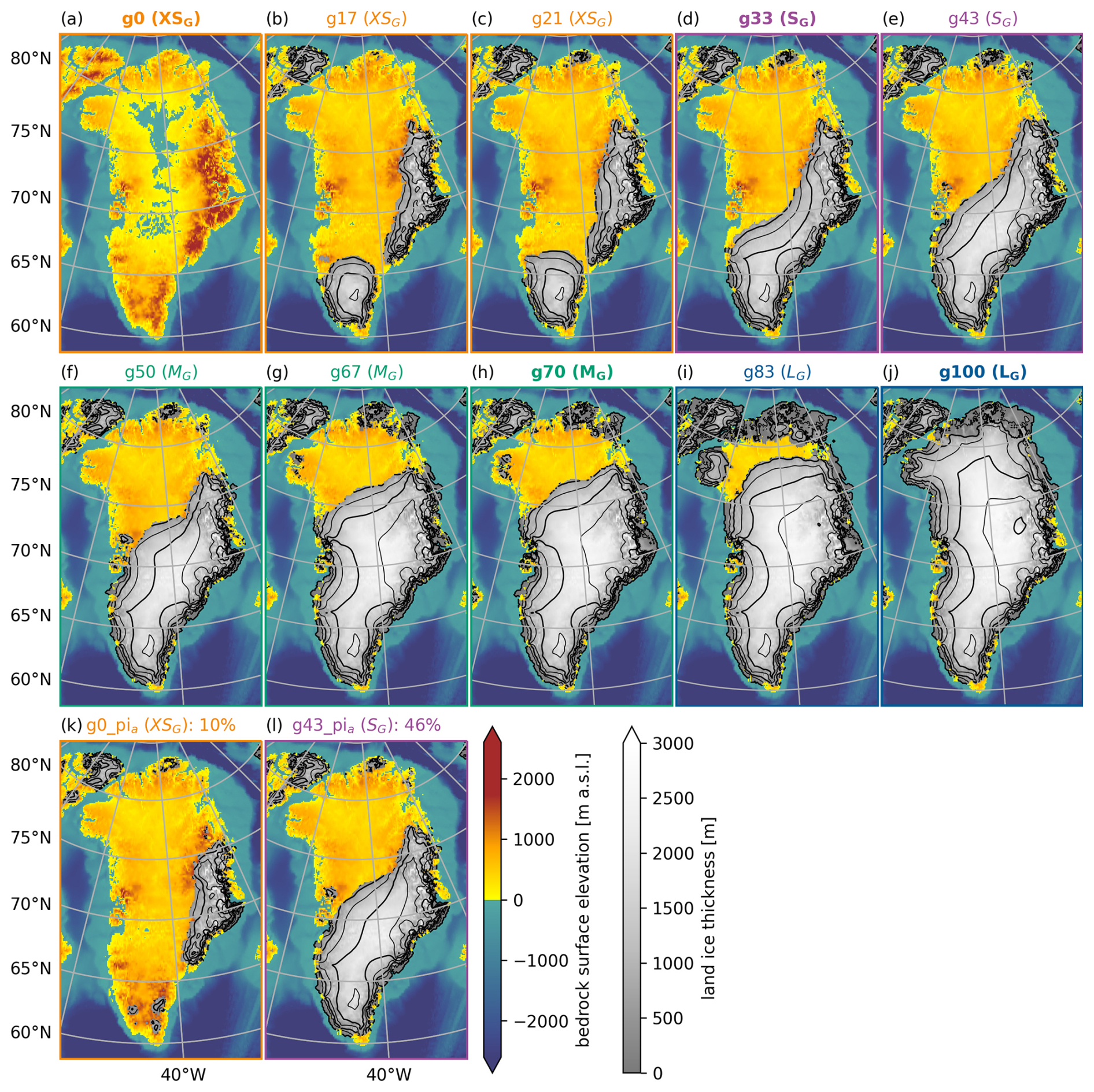
Figure A1 Maps of GrIS ice thickness used as initial GrIS in the experiments described in Sect. 2.2 overlaid on the surface bedrock in meters above sea level ($\mathrm{m}\mathrm{a}.\mathrm{s}.\mathrm{l}.$) for the respective state. The first and second row show the initial GrIS in the ten main simulations. Experiment names indicate the initial GrIS volumes (e.g., g43 was initialized with a GrIS volume of 43 %). The last row shows the initial GrIS in the sensitivity experiments, which were branched off g0 and g43 and run with a prescribed PI AIS. Colors of the titles, state names in parentheses and frames refer to the final steady states in Fig. 2. The simulations used for the main analysis of the steady states are highlighted in bold font.

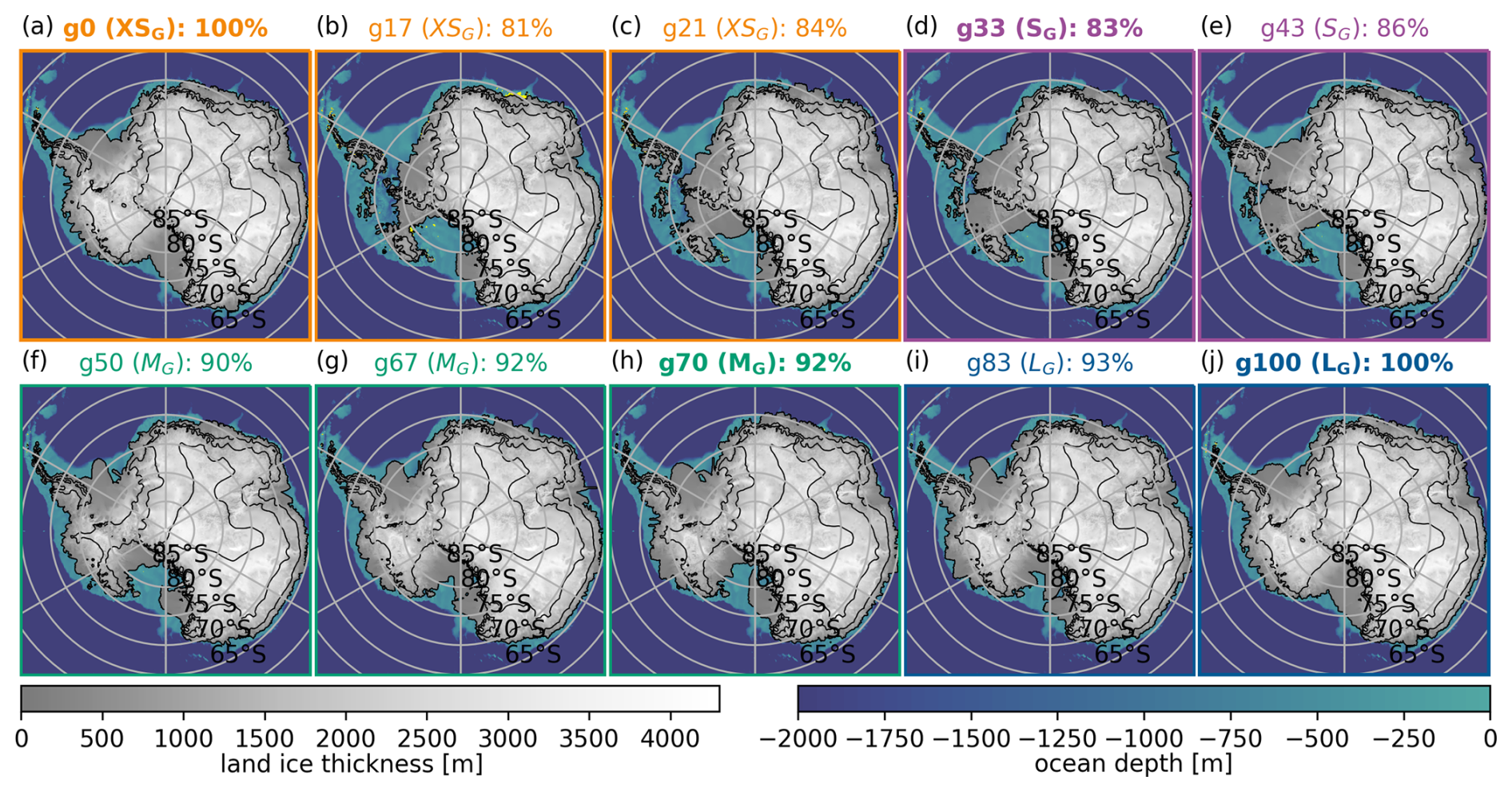
Figure A2 Similar to Fig. A1 but for the AIS. The titles indicate (1) the name of the simulation, (2) the final GrIS state, and (3) the initial AIS volume.

Appendix B: Disentangling the feedbacks and processes between the GrIS and the climate system that stabilize the steady states

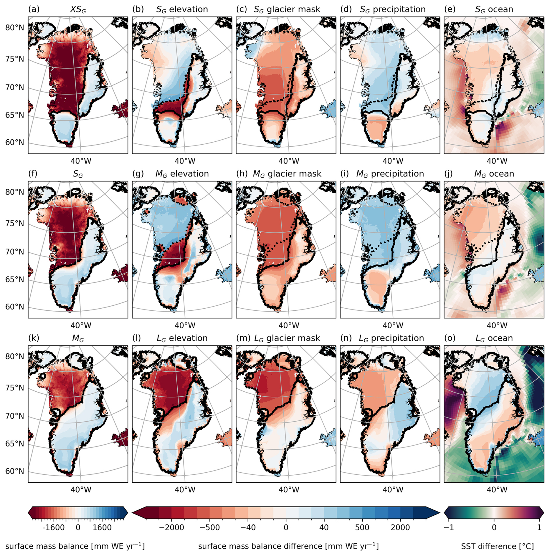
Figure B1 Maps of SMB indicating the contribution of the different feedbacks and processes between the GrIS and the climate system to stabilize each state. The left column shows the absolute SMB field of each steady state. The remaining columns show the difference between the SMB field derived for each state and the SMB field derived for the state but including the impact of imposing the neighboring state that is indicated in the figures' title. A positive SMB indicates that the respective factor favors maintaining the state or even an ice sheet expansion, thus is stabilizing. A negative SMB indicates that the respective factor impedes an ice sheet expansion or even favors retreat, thus is destabilizing. The solid black line indicates the glacier mask of the respective steady state and the dashed black line of the next larger steady state. The spatial averages presented in Fig. 7 are computed for the non-overlapping area between the two different glacier masks in central Greenland, excluding scattered coastal grid cells. Note that glacier mask also includes the albedo feedback. The far-right column also displays the SST difference of the smaller minus the larger state.

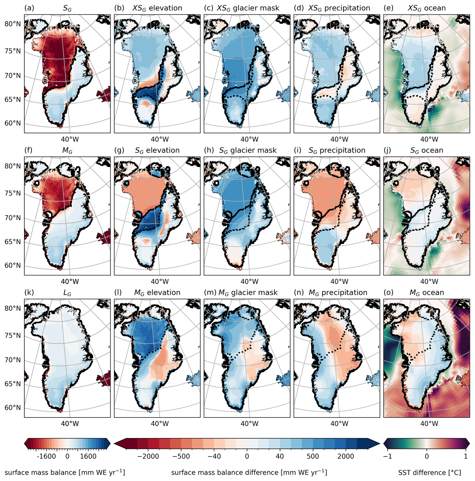
Figure B2 Similar to Fig. B1 but for the neighboring smaller state.

Appendix C: Rapid state transition in XS_G

In year 30 000, a rapid transition from a smaller into the steady XS_G occurs in g0 (Fig. 2). This transition occurs when individual glaciers in the south of Greenland connect to form a single larger ice sheet. To identify the driver of this rapid transition, we designed additional sensitivity experiments. First, we investigated whether climate variability is driving the transition. For this, we designed an experiment that was branched off from g0 shortly before the transition occurs (year 28 050) and run with SST and SSS nudged towards the average climate conditions of the 800 model years preceding the transition in g0. It is referred to as g0_g0_oce_transition. Hence, this experiment includes altered ocean dynamics but reduced climate variability. The transition to a larger GrIS occurs also with a reduced climate variability in g0_g0_oce_transition. This indicates that climate variability is not the driver of the transition. Second, we investigated whether certain ocean conditions in response to an absent or smaller GrIS drive the transition by conducting another sensitivity experiment (g0_g100_oce_transition), branched off in the same year as g0_g0_oce_transition, but with ocean nudging towards the g100 climatology that features a PI GrIS. The rapid transition is present in the sensitivity experiment using the ocean conditions of the large GrIS (g0_g100_oce_transition). This suggests that once the glaciation has been initiated by colder ocean temperatures in the Nordic Seas in the XS_G state in g0 (as described in Sect. 3.2), the ice sheet regrowth becomes self-amplifying, independent of the oceanic conditions. These additional sensitivity experiments show that ice sheet regrowth in the south of Greenland is initiated by the colder ocean conditions in the XS_G state in g0 compared to the L_G state in g100 (compare experiment g0_pi_oce in Sect. 3.2), while the rapid transition around year 30 000 is driven by ice dynamics and occurs independent of the changes in the ocean.