Extended seasonal prediction of Antarctic sea ice concentration using ANTSIC-UNet

Antarctic sea ice has experienced rapid change in recent years, with the total sea ice extent abruptly decreasing after a period of gradual increase from the late 1970s until 2014. Accurate long-term predictions of Antarctic sea ice concentration by dynamical or machine learning models are crucial for supporting the expanding activities in the Southern Ocean, related to for instance scientific research, tourism and fisheries. However, dynamical models often face difficulties in accurately predicting Antarctic sea ice due to limited representations of air-ice-sea interactions, especially on seasonal timescales and during the summer months. In addition, existing deep learning approaches typically rely on historical sea ice data, neglecting the complex interactions between sea ice and other climate variables, and lack interpretability of the underlying physical processes. Moreover, little attention has been paid to extended seasonal forecasts, and systematic evaluations of the predictive skill during extreme years remain scarce. To address these challenges and gaps, we here develop a deep learning model (named ANTSIC-UNet), trained by multiple climate variables, and evaluate its skill for extended up-to-six-months seasonal prediction of Antarctic sea ice concentration. We compare the predictive skill of ANTSIC-UNet in the Pan- and regional Antarctic with two benchmark models (a linear trend and an anomaly persistence model) and a dynamical model (SEAS5). In terms of root-mean-square error (RMSE) of sea ice concentration and integrated ice-edge error (IIEE), ANTSIC-UNet shows much better skills relative to the other models for the extended seasonal prediction, especially for the extreme events in recent years. Sea ice prediction errors increase with lead time, and are smaller during autumn and winter than in summer. The Pacific and Indian Oceans show accurate prediction performance at the sea ice edge during summer, and ANTSIC-UNet provides high predictive skill in capturing the interannual variability of Pan-Antarctic and regional sea ice extent anomalies. In addition, we quantify the importance of variables through a post-hoc interpretation method. This analysis suggests that the ANTSIC-UNet prediction at short lead times is sensitive to sea surface temperature, radiative flux, and atmospheric circulation in addition to sea ice conditions. At longer lead times, zonal wind in the stratosphere appears to be an important influencing factor for the prediction. Building on these findings, we further demonstrate that incorporating physical constraints into deep learning models potentially leads to a gain in the accuracy of the Antarctic sea ice edge prediction on extended seasonal timescales.

1 Introduction

Sea ice affects the climate system through modulating the exchange of radiation, heat, momentum, moisture and gases between the atmosphere and ocean. Antarctic sea ice is an essential component of the climate system. It strongly affects the local atmosphere and ocean and the extrapolar Southern Hemisphere through dynamical and thermodynamic processes, particularly in a warming climate (Massom and Stammerjohn, 2010; Kidston et al., 2011; Abernathey et al., 2016; Zhu et al., 2023). The summer total Antarctic sea ice extent (SIE) has gradually increased until 2014 since the late 1970s and then abruptly decreased (Turner et al., 2013; Hobbs et al., 2016; Comiso et al., 2017; Fogt et al., 2022; Liu et al., 2023). Antarctic SIE shows large seasonal and interannual variability, with trends that are spatially heterogeneous (Liu et al., 2004; Raphael and Hobbs, 2014; Libera et al., 2022). Sea ice in different regions exhibits complex spatial patterns of change in growth, retreat, and duration (Liang et al., 2023). The Southern Ocean sea ice region is divided into five sectors: the Weddell Sea, Indian Ocean, Pacific Ocean, Amundsen and Bellingshausen Seas, and Ross Sea. These regions are characterised by their unique climatic, oceanographic, and geographical characteristics (Zwally et al., 2002; Grieger et al., 2018; Josey et al., 2024). This division has been widely used in studying the regional dynamics and prediction of Antarctic sea ice (e.g., Eayrs et al., 2019; Bushuk et al., 2021; Liang et al., 2023).

Compared to the Arctic, the prediction of Antarctic sea ice has received much less attention. Yet subseasonal to extended seasonal Antarctic sea ice predictions are increasingly demanded due to the expanding range of activities in the Southern Ocean (Zampieri et al., 2019; Bushuk et al., 2021; Libera et al., 2022). Accurate sea ice concentration predictions can provide early warnings about sea ice changes and related hazards. This is particularly important for managing the risks of shipping activities in the Southern Ocean. For example, two polar vessels, Akademik Shokalskiy and Xuelong became trapped in rapidly formed sea ice in the Antarctic coastal region (Wang et al., 2014). Commercial fishing and tourism operations mostly use ice-strengthened vessels rather than icebreakers, which are vulnerable to sea ice hazards. Improved predictions will support ecosystem management and inform policy decisions, since the seasonal variations in Antarctic sea ice have a profound influence on marine productivity and fisheries (Libera et al., 2022).

Statistical models, such as the Markov model (e.g., Chen and Yuan, 2004; Pei, 2021) and the Koopman mode decomposition model (Hogg et al., 2020), have been employed to forecast seasonal Antarctic sea ice concentration. However, these statistical models were inferior to the anomaly persistence model for some seasons and regions. Additionally, there have been limited efforts to forecast seasonal Antarctic sea ice using dynamical models due to the challenges associated with faithfully simulating complex air-ice-sea interaction processes in the Southern Ocean (Morioka et al., 2019; Bushuk et al., 2021). Dynamically, sea ice movement and deformation are driven by wind and ocean currents. Thermodynamically, sea ice melting and formation are influenced by convection associated with ocean vertical mixing, heat exchange driven by surface radiation budget and turbulence, and heat advection through horizontal transport of air and water masses. However, most dynamical forecast systems overestimate the extent of the Antarctic sea ice edge at the sub-seasonal scale with their predictive skill falling below climatological benchmarks (Zampieri et al., 2019). Starting in 2017, the Sea Ice Prediction Network South (SIPN South) has coordinated the evaluation of forecasting methods and systems used to predict summer Antarctic sea ice (Massonnet et al., 2023). The evaluation reveals that both statistical and dynamical models have substantial biases and ensemble spread.

In recent years, deep learning (DL) methods have been widely used for Arctic sea ice prediction at various temporal scales (e.g., Chi and Kim, 2017; Fritzner et al., 2020; Kim et al., 2020; Ren and Li, 2021). Andersson et al. (2021) introduced IceNet to predict probabilities of Arctic sea ice edge with uncertainty quantification. Ren and Li (2023) developed a DL method with a physically constrained loss function to improve Arctic sea ice predictions at lead times of 90 d. However, very limited effort has been made to apply DL methods to Antarctic sea ice prediction and associated assessments are still at an early stage. For the SIPN South summer Antarctic sea ice extent forecast (Massonnet et al., 2023), one contributor provided the prediction using a k-nearest neighbors (KNN) method. Recently, Wang et al. (2023) developed a SIPNet model with encoder-decoder structure for subseasonal Antarctic sea ice concentration prediction, which outperforms some dynamical models and advanced linear statistical models at lead times of 1–8 weeks. Dong et al. (2024) employed a convolutional long short-term memory (ConvLSTM) network to predict Antarctic SIC up to 60 d ahead, which shows skillful predictions within 30 d and accurately forecasts annual maximum and minimum sea ice extents from 2017 to 2022. However, ConvLSTM demands significant computational resources during training, and relies on iterative forecasting which leads to error accumulation over time and requires a trade-off between accuracy and prediction length. Lin et al. (2025) proposed Ice-KNN-South, a lightweight machine learning model for predicting daily Antarctic SIC at lead times of 1–90 d. While these studies have made significant contributions, they primarily rely on historical SIC data without considering underlying physical processes governing the variation of Antarctic sea ice. Furthermore, they focus on shorter prediction horizons, and their skillfulness in extended seasonal forecasting remains unknown.

The purposes of this study are to (1) develop a DL model, named ANTSIC-UNet, to achieve extended seasonal prediction of Antarctic sea ice concentration by considering not only the sea ice itself but also a wealth of variables associated with ocean-ice-atmosphere interactions, (2) assess the predictive skill of ANTSIC-UNet for both Pan- and regional Antarctic sea ice, especially for recent extreme years, (3) apply a post-hoc interpretation method to quantify the variable importance that affects sea ice predictability, and (4) explore the incorporation of physical constraints into the DL model to improve the accuracy of Antarctic sea ice edge predictions.

2 Data and Method

2.1 Data

In this study, monthly Antarctic sea ice concentration (SIC) data obtained from the National Snow and Ice Data Center (NSIDC) (https://nsidc.org/data/nsidc-0079/versions/3, last access: 8 April 2025) are used as the input of ANTSIC-UNet, and are derived from brightness temperature of the Scanning Multichannel Microwave Radiometer (SMMR), the Special Sensor Microwave/Imager (SSM/I) sensors, and the Special Sensor Microwave Imager/Sounder (SSMIS). SIC is retrieved using the Bootstrap algorithm, which utilizes brightness temperature (Tb) observations from the 37H, 37V, and 19V channels to estimate sea ice concentration (Comiso et al., 1997; Comiso and Nishio, 2008). The SIC data have a size of 332×316 grid points with a spatial resolution of 25km, spanning from 1979 to 2023.

Long-term observations are scarce in the Antarctic, which cannot provide the comprehensive and consistent three-dimensional and time-evolving gridded field of atmosphere and ocean parameters necessary to understand sea ice changes. Reanalysis datasets, which assimilate observations and satellite data, are valuable tools for investigating climate changes in polar regions, offering multivariate descriptions of atmospheric and oceanic conditions. ECWMF Reanalysis v5 (ERA5, Hersbach et al., 2020) provides high-resolution and three-dimensional gridded data of comprehensive atmospheric variables from 1940 to the present. ERA5 and its predecessor ERA-Interim are widely regarded as the best-performing reanalysis datasets in polar regions, with particularly reliable analyses over the Southern Ocean compared with surface and upper-level observations (Bracegirdle and Marshall, 2012; Bromwich et al., 2011). Ocean Reanalysis System 5 (ORAS5, Zuo et al., 2019) is a global eddy-permitting ocean and sea-ice ensemble reanalysis which provides historical ocean and sea-ice conditions from 1979 to the present, and is based on the assimilation of the same sea surface temperature observations as is the case of ERA5. Sea ice changes are strongly influenced by the atmosphere above and the ocean below through dynamical and thermodynamic processes. Therefore, the relevant atmospheric variables selected from ERA5 and oceanic variables obtained from ORAS5 are also used as inputs by ANTSIC-UNet to investigate the key factors contributing to sea ice predictions in the complex interaction between sea ice, ocean and atmosphere. These variables are listed in Table 1 and include 2 m air temperature (T2), 500 hPa air temperature (T500), sea surface temperature (SST), ocean temperature (PT), ocean heat content for the upper 300 m (OHC300), downwelling solar radiation (DSR), upwelling solar radiation (USR), sea level pressure (SLP), 500 hPa geopotential height (H500), 250 hPa geopotential height (H250), 10 m u-component of wind (U10), 10 m v-component of wind (V10), and 10 hPa zonal wind (U10 hPa). The averaged ocean temperature at different depths in the upper Southern Ocean, 50–100 m (PT50) and 100–150 m (PT100), has been calculated. Before integrating into ANTSIC-UNet, these variables are bilinearly interpolated to the NSIDC sea ice polar stereographic grid and normalised. Additionally, a land mask obtained from the NSIDC is used for the consistency of SIC and other variables.

The input vector is a 3-dimensional matrix with the size of $\mathrm{332}\times \mathrm{316}\times \mathrm{57}$. The dimension with 57 elements represents all variables mentioned above, including sea ice concentration for the past 12 months, the linear trend prediction of sea ice concentration for the following 6 months, 12 climate variables for the past 3 months, 2 climate variables for the past 1 month, and the land mask. All variable fields are mapped on 332×316 grids (see Table 1 for the details of all input variables). The final output provides the 6-month forecast of monthly Antarctic sea ice concentration.

Table 1 The information of all input variables for ANTSIC-UNet.

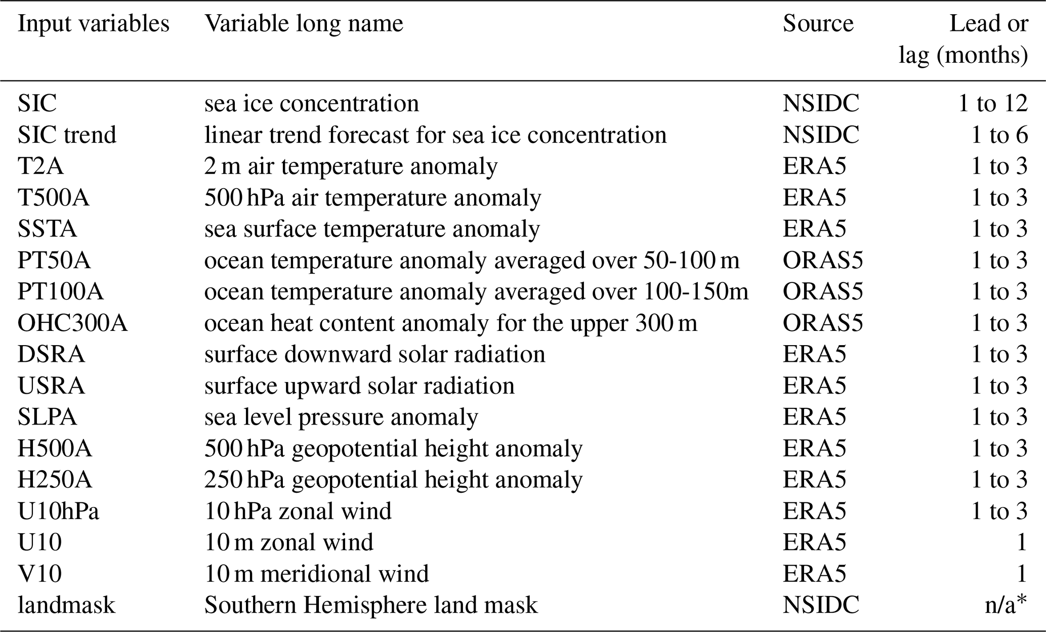
^* n/a: not applicable.

2.2 ANTSIC-UNet model

In this study, we construct an ensemble deep learning model, aiming at providing seasonal six-months Antarctic sea ice concentration prediction. The ANTSIC-UNet consists of 20 members possessing the encoder and decoder structure associated with a fully convolutional network (Fig. 1). A U-shaped architecture based on convolutional neural networks is widely used for many applications, i.e., remote sensing image segmentation tasks (Marmanis et al., 2016; Wang et al., 2023). Recently, Andersson et al. (2021) employed the U-Net for three-class predictions of Arctic sea ice concentration. For accurate forecasts of Antarctic sea ice concentration, we made necessary modifications to the original architecture of U-Net and turned it into single value regression rather than the classification. The ANTSIC-UNet's inputs are feature maps of high-resolution sea ice concentration and other multiple climate variables related to sea ice changes over different lead/lag months and a land mask. The outputs are high-resolution sea ice concentration maps for the future months. To avoid deformation, we resize the spatial shape to a 336×320 grid, by applying the nearest neighbor method, before input to the encoder, and we adopt a padding technique to avoid too much data reduction. The inputs are processed into a large number of feature maps with decreased dimensionality by the encoder part of ANTSIC-UNet. Such deep layers and large-scale features allow the model to capture complex nonlinear relationships and provide an interpretation of the inputs. The decoder then upscales the feature maps extracted by the encoder into upsampled features and uses four skip connections to combine them with multi-scale features from different scale levels of the encoder. This process results in high-resolution output maps that align with the spatial dimensions of the input data. Finally, sigmoid activation functions are used in the last six convolutional layers, and the output module extracts slices with dimensions of 332 × 316 × 6, which generate the regression predictions for Antarctic sea ice concentration maps over a six-month period.

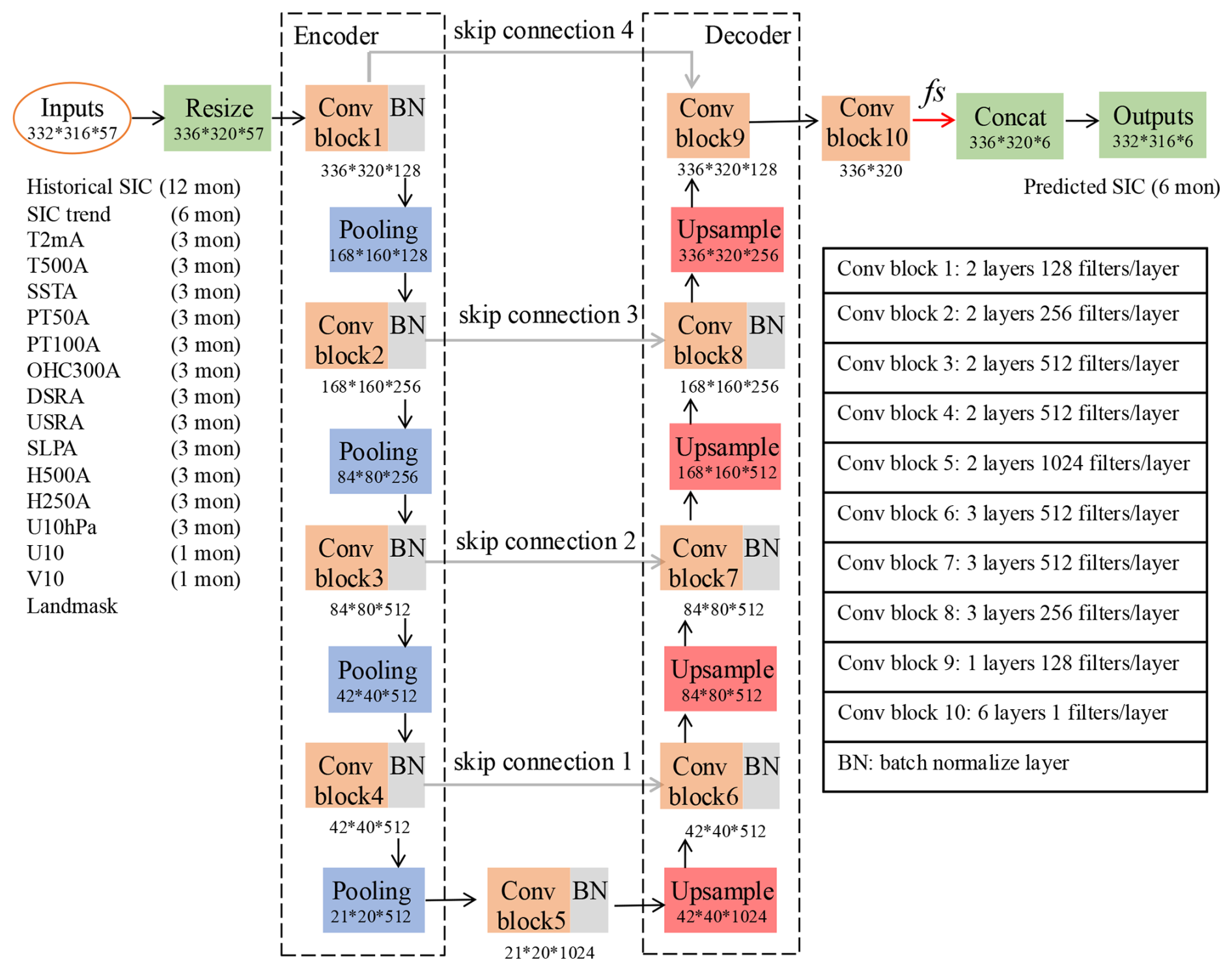
Figure 1 Configuration of ANTSIC-UNet model used for extended seasonal Antarctic sea ice prediction. Inputs are sea ice concentration, other climate variables related to sea ice changes over different lead/lag months and a land mask. The U-shaped architecture includes the encoder, decoder and four skip connections. Sigmoid activation functions (fs) are used in the final six convolutional layers to generate regression predictions of Antarctic sea ice concentration maps for six months.

We divide the data into three groups: the training data from 1979 to 2011, the validation data from 2012 to 2019 (with exclusion years 2014 and 2017), and testing data in 2017, from 2020 to 2023 (anomalously low extent period) and 2014 (record high) for independent evaluation. An early stopping strategy is adopted to avoid overfitting when the performance on the validation data does not improve after 10 epochs as suggested by Prechelt (2012). The testing data do not participate in the training process so that the performance of the testing data provides an independent assessment of ANTSIC-UNet' ability to generalize to new data. Here, we use typical hyperparameters for the deep learning model. The kernel size for the convolutional layers is set to (3,3). Due to memory constraints, we set the batch size to 2. The loss function applied is mean squared error (MSE), with a learning rate of 0.0001 and a weight decay of 0. The Adam optimizer is used for training.

2.3 Benchmark models

In this study, the linear trend and anomaly persistence predictions are used as benchmarks to assess the predictive skill of ANTSIC-UNet. The linear trend model involves fitting a linear least-squares trend to observed SIC over the past 30 years at each grid cell for each calendar month. This trend is then used to predict SIC values for the corresponding calendar month in the following year. Additionally, these SIC predictions from this linear trend model are also used as the input to ANTSIC-UNet.

The anomaly persistence prediction is calculated as follows:

$$\begin{array}{}\text{(1)}& {\mathrm{SIC}}_{\mathrm{pred}}\left(t+\mathit{\tau }\right)={\mathrm{SIC}}_{\mathrm{clim}}\left(t+\mathit{\tau }\right)+{\mathrm{SIC}}_{\mathrm{anom}}\left(t\right)\end{array}$$

where SIC_pred is the target month predicted ice concentration at the lead time τ, SIC_clim is the climatogy ice concentration at the target month, and SIC_anom is the observed ice concentation anomaly relative to the climatology at the initial time. The climatology for each month is computed for the period of the training data (1979–2011). The anomaly persistence works by preserving the deviations from the climatological anomalies and assuming these anomalies will persist into the future. For example, if a particular region currently has more sea ice than average, this positive anomaly will continue as time progresses. This statistical method has been widely used as a benchmark for predicting sea ice concentration on seasonal timescales, since sea ice conditions often change gradually rather than abruptly (Wayand et al., 2019; Bushuk et al., 2021; Niraula and Goessling, 2021). While this method is effective for short-term forecasts, its accuracy declines over longer lead times as the influence of initial anomalies weakens.

To further assess the Antarctic sea ice predictive skill of ANTSIC-UNet against other prediction efforts, we included a dynamical model's monthly mean Antarctic sea ice concentration predictions calculated by the ensemble mean of 51 members of SEAS5, provided by the Copernicus Climate Change Service (C3S) Prediction project (Thépaut et al., 2018). SEAS5, ECMWF's fifth-generation seasonal forecast system, is recognized for its state-of-the-art predictive skill among the dynamical models which provides Antarctic sea ice concentration prediction for up to six months (Johnson et al., 2019).

2.4 Evaluation metrics

We quantify the predictive skill of both the Pan- and regional Antarctic sea ice using four metrics: (1) root-mean-square error (RMSE), (2) anomaly correlation coefficient (ACC), (3) mean squared error skill score (MSSS), and (4) integrated ice-edge error (IIEE). RMSE reflects the proximity between the prediction and observation. ACC is a measure of the accuracy of the prediction anomalies based on the relationship between the predicted and observed deviation from their respective climatologies (Wang et al., 2016). MSSS is a skill score based on a comparison between the model predictions and climatology which are considered as a reference forecast. The value of MSSS varies from negative infinity to 1, with a negative value indicating no predictive skill and below the reference forecast (due to deviations from observations being larger than observed annual fluctuations), and 1 indicating a perfect forecast (Murphy, 1988). Here we use ACC = 0.5 and MSSS = 0.0 as the lowest limit for predictive skill, which is widely used in previous research (e.g., Goddard et al., 2012; Choi et al., 2016; Bushuk et al., 2021). The integrated ice-edge error (IIEE) is a verification metric for sea ice forecasts representing the sum of overestimated and underestimated sea ice extent where sea ice concentration > 15 % (Goessling et al., 2016). These metrics are calculated as follows:

$$\begin{array}{}\text{(2)}& {\displaystyle }\mathrm{RMSE}=\sqrt{\mathrm{MSE}}=\sqrt{\mathrm{mean}\left(\right(p-o{)}^{\mathrm{2}})},\text{(3)}& {\displaystyle }\mathrm{ACC}={\displaystyle \frac{\sum (p-\stackrel{\mathrm{‾}}{p})(o-\stackrel{\mathrm{‾}}{o})}{{\sqrt{\sum (p-\stackrel{\mathrm{‾}}{p})}}^{\mathrm{2}}\sqrt{\sum (o-\stackrel{\mathrm{‾}}{o}{)}^{\mathrm{2}}}}},\text{(4)}& {\displaystyle }\mathrm{MSSS}=\mathrm{1}-{\displaystyle \frac{{\mathrm{MSE}}_{\mathrm{pred}}}{{\mathrm{MSE}}_{\mathrm{clim}}}}=\mathrm{1}-{\displaystyle \frac{\sum (p-o{)}^{\mathrm{2}}}{\sum (\stackrel{\mathrm{‾}}{o}-o{)}^{\mathrm{2}}}},\text{(5)}& {\displaystyle }\mathrm{IIEE}={\mathrm{SIE}}_p\cup {\mathrm{SIE}}_o-{\mathrm{SIE}}_p\cap {\mathrm{SIE}}_o,\end{array}$$

where p is the predicted ice concentration or sea ice extent by ANTSIC-UNet and o is the observed ice concentration or ice extent; $\stackrel{\mathrm{‾}}{p}$ and $\stackrel{\mathrm{‾}}{o}$ are the mean of the prediction and observation.

2.5 Variable importance analysis

We use the permutation feature importance approach to determine which variables are important for Antarctic sea ice prediction in ANTSIC-UNet. This method was introduced by Breiman (2001) and Fisher et al. (2019) to interpret the model's decisions. Specifically, when a particular variable is selected, the original input feature matrix is X_orig and the permutation feature matrix is X_perm. The evaluation metric e_i,j used is the root-mean-square error (RMSE) between the output f_i,j (the predicted SIC by the trained model for the target month at the lead time ranging from 1 to 6 months) and the target Y_i (observed SIC) for a given month. Thus, the feature importance value FI_i,j is defined as the accuracy change of the evaluation metric where i refers to the target month to be predicted and j refers to the lead month.

$$\begin{array}{}\text{(6)}& {\mathrm{FI}}_{i,j}=e_{i,j}^{\mathrm{perm}}-e_{i,j}^{\mathrm{orig}},\end{array}$$

where

$$\begin{array}{}\text{(7)}& {\displaystyle }{e}_{i,j}^{\mathrm{orig}}=\mathrm{RMSE}\left({\mathbf{Y}}_i;f_{i,j}\left({\mathbf{X}}_{\mathrm{orig}}\right)\right),\text{(8)}& {\displaystyle }{e}_{i,j}^{\mathrm{perm}}=\mathrm{RMSE}\left({\mathbf{Y}}_i;f_{i,j}\left({\mathbf{X}}_{\mathrm{perm}}\right)\right),\end{array}$$

The importance of each particular variable is measured by (1) randomly shuffling the variable across spatial grids and replacing it in the original input vector to generate a new input vector, and (2) calculating the error of the evaluation metric after permuting the variable. The positive increase of FI_i,j means that the variable is important, and no change and decrease of FI_i,j indicates that the variable plays little role. Here we iteratively shuffle each input variable and compare the performance, and repeat the procedure 10 times. The mean feature importance value is calculated with the testing data for the period of 2020–2023.

3 Results

3.1 Pan-Antarctic and regional predictive skill

Pan-Antarctic sea ice concentration predictions from ANTSIC-UNet, statistical models (linear trend and anomaly persistence models) and dynamical model (SEAS5) for the testing years averaged for all lead times are shown in Table 2. Overall, ANTSIC-UNet has the smallest SIC RMSE and significantly reduced IIEE compared to other models. In order to consider the variations of the metrics results with lead times and different regions, we compare the three models for lead times ranging from 1 to 6 months for the Pan-Antarctic and five sub-regions (Fig. 2). For ANTSIC-UNet, SEAS5 and anomaly persistence model, both RMSE and IIEE grow with increasing lead time, reflecting a decrease of predictive skill for the extended seasonal forecast. Compared to the SEAS5 and anomaly persistence model, ANTSIC-UNet exhibits significantly lower RMSE over the entire Antarctic and all sub-regions for all lead times, except for the Indian Ocean, where its error is slightly higher than that of anomaly persistence model for lead time exceeding 3 months. In addition, RMSE of ANTSIC-UNet also exceeds the linear trend model when the lead time exceeds 3 months, which is due to the reduced predictive skill in the Indian Ocean, Pacific Ocean, Amundsen and Bellingshausen Seas. Encouragingly, the IIEE of ANTSIC-UNet is consistently smaller than that of the two benchmark models and SEAS5 for the Pan-Antarctic, though it is comparable to the linear trend model for lead times exceeding 3 months in the Amundsen and Bellingshausen Seas. SEAS5 shows the smallest IIEE in the Ross, Amundsen and Bellingshausen Seas at 1-month lead, but the errors grow substantially with lead time and exceed those of ANTSIC-UNet. The superior skills in sea ice edge predictions of ANTSIC-UNet become more pronounced as the lead time increases. Overall, ANTSIC-UNet shows high predictive skill in the Weddell and Ross Seas, outperforming the two benchmark models and SEAS5.

Table 2 The averaged predictive skill of Antarctic sea ice for ANTSIC-UNet, statistical models (linear trend and anomaly persistence models) and SEAS5 for all testing years (RMSE: root-mean-square error; IIEE: integrated ice-edge error).

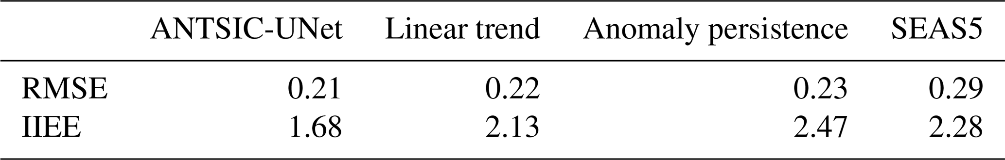
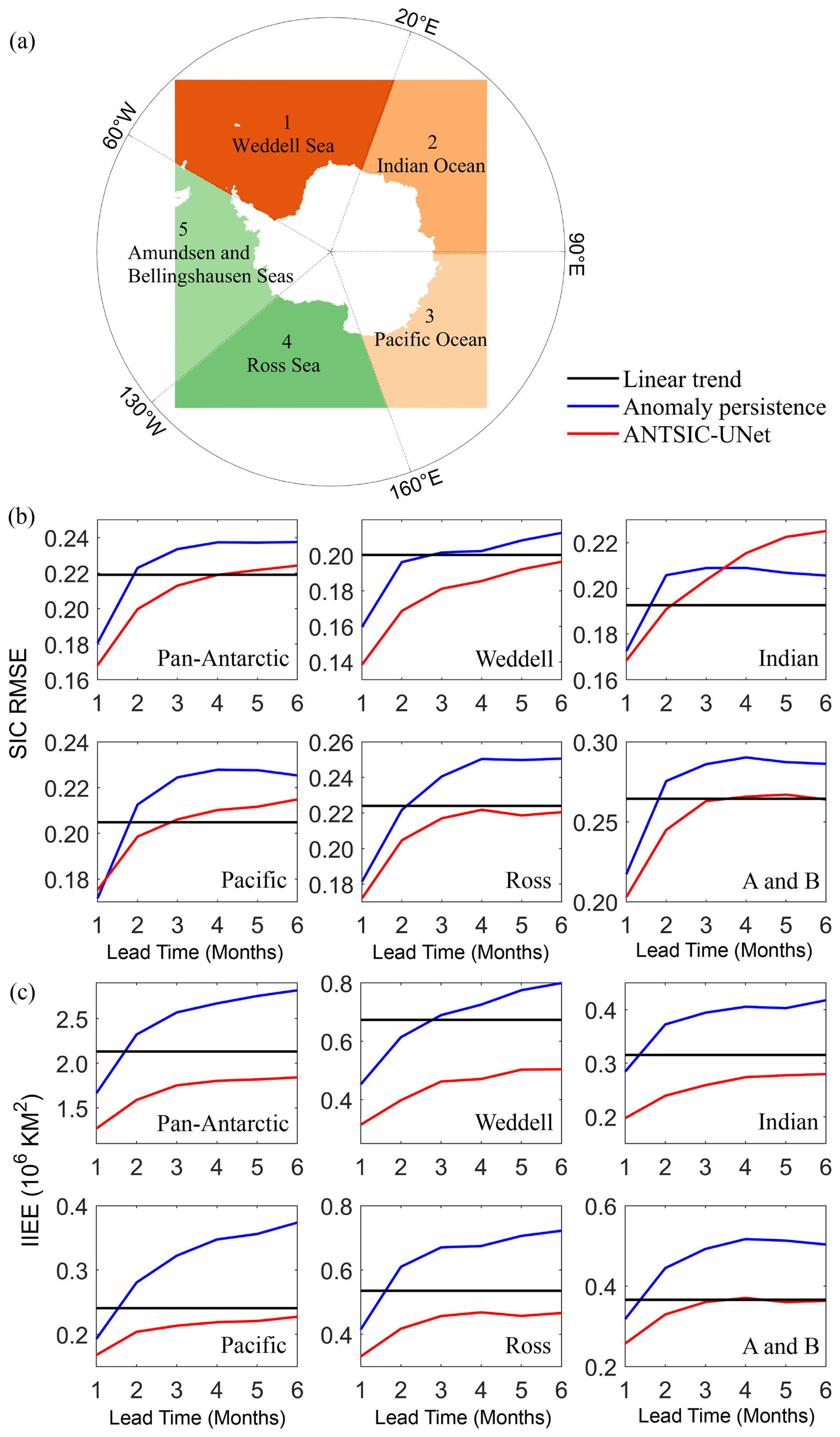
Figure 2 (a) Domian of sub-regions: 60° W–20° E (Weddell Sea), 20–90° E (Indian Ocean), 90–160° E (Pacific Ocean), 160° E–130° W (Ross Sea), and 130–60° W (Amundsen and Bellingshausen Seas). (b) and (c) the averaged predictive skill of Pan- and regional Antarctic sea ice for ANTSIC-UNet, linear trend model, anomaly persistence model and SEAS5 predictions. (b) SIC RMSE and (c) IIEE. Note that the prediction with the linear-trend model is based on the same calendar month one year before and is hence independent of lead time.

Figure 3 shows the spatial distribution of February and September SIC. In February (seasonal minimum), the linear trend model overestimates SIC in the Ross Sea and western and central Weddell Sea and underestimates SIC in the Amundsen and Bellingshausen Seas. Compared to the linear trend model, the anomaly persistence model has relatively small biases at 1-month lead. However, the magnitude and coverage of the biases become larger as the lead time increases and are large positive (negative) biases in parts of the eastern Pacific sector (the Indian sector) at 5-month lead. Moreover, the anomaly persistence model leads to an unrealistic northward expansion of the biases, as the initial spring months cover a broader area of sea ice than the target month. SEAS5 underestimates SIC, and the negative biases increase with lead time, particularly in the western Weddell Sea and the Pacific Ocean. By contrast, the ANTSIC-UNet prediction shows the smallest biases (mostly negative across much of the Antarctic) at 1-month lead. As the lead time increases, the magnitude of the biases gradually increases, except that the negative bias in the Ross Sea changes to become positive. In September (seasonal maximum), the linear trend and anomaly persistence (at 1-month lead) models tend to have alternating negative and positive biases near the sea ice edge. SEAS5 shows large negative biases over the entire Antarctic sea ice region, with alternating positive and negative biases emerging at the sea ice edge zone as lead time increases. By contrast, the ANTSIC-UNet prediction has smaller and mostly negative biases across much of the Antarctic at 1-month lead. As the lead time increases, both the ANTSIC-UNet and anomaly persistence models show biases becoming larger in the sea ice edge zone. Moreover, large biases also appear in the compact ice zone for the anomaly persistence model.

To further evaluate the spatial performance of ANTSIC-UNet, Fig. 4 shows the averaged SIC RMSE and IIEE between the ANTSIC-UNet predictions and observations for each target month and different lead times. In terms of RMSE, Pan-Antarctic exhibits low values from autumn to spring (from April to November), though there is an increase in RMSE during summer months (from December to March) as the lead time exceeds 2 months. In terms of IIEE, Pan-Antarctic has small values at 1-month lead, which extend to 2–3 month lead in February and March. In general, the values of IIEE increase as lead times increase, and large values occur from November to January as the lead time exceeds 2–3 months. As shown in Fig. 4b1–f1, the large values of RMSE are also found in summer for all sub-regions, but relatively small values are found in the Weddell Sea. For IIEE in Fig. 4b2–f2, all sub-regions show similar distributions, except that the low IIEE in the Indian and Pacific Oceans have broader coverage. Increased IIEEs are found in the Weddell Sea (Ross Sea) from November to January (from December to March) as the lead time exceeds 2–3 months. Overall, the Pacific and Indian Oceans show better predictive skills at the sea ice edge zone in summer relative to other regions.

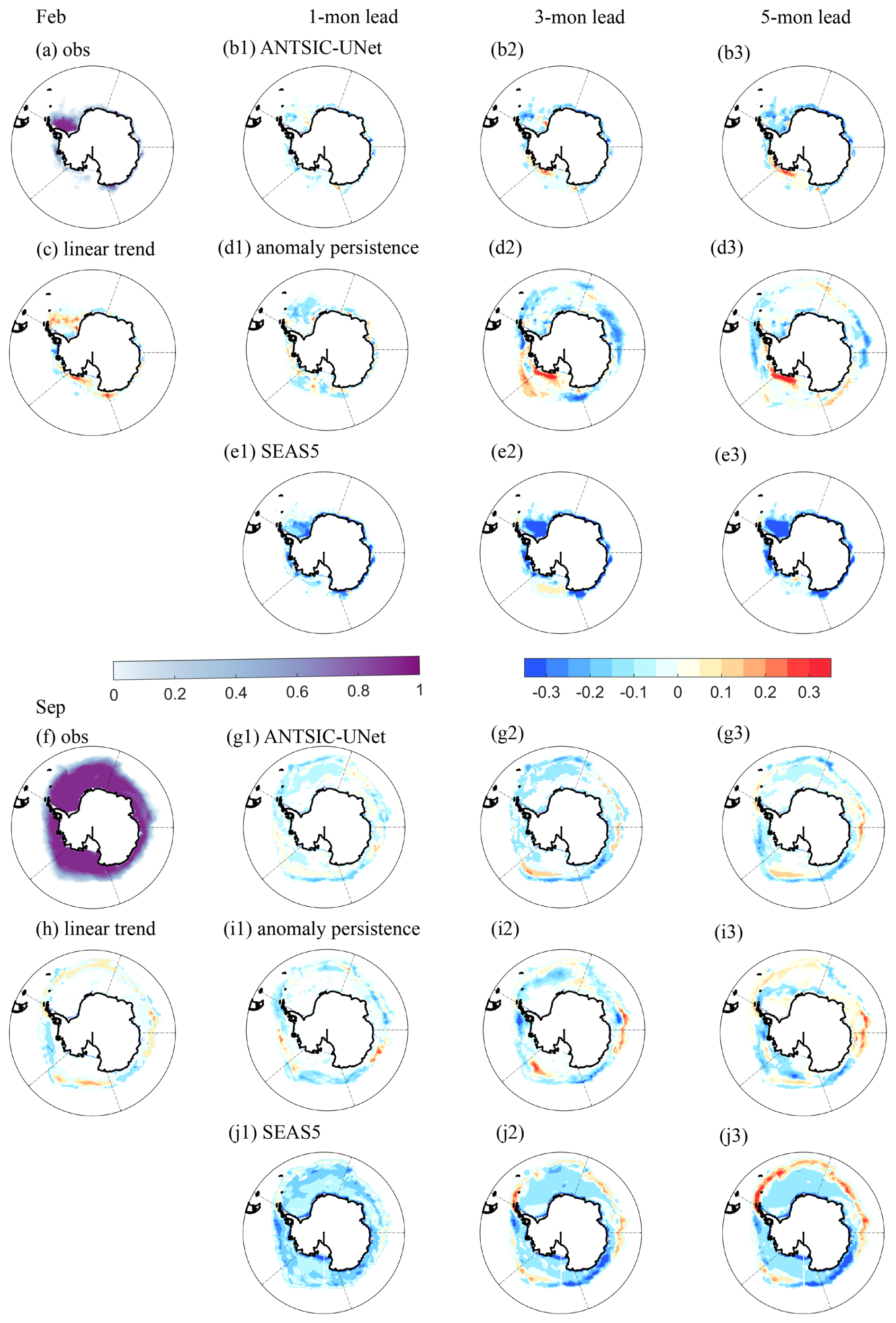
Figure 3 The monthly mean sea ice concentration of the NSIDC observations for (a) February and (f) September, and the errors in predicting by ANTSIC-UNet (b1–b3, g1–g3), the linear trend model (c, h), anomaly persistence model (d1–d3, i1–i3) and SEAS5 (e1–e3, j1–j3) at lead time of 1, 3, and 5 months for February (upper panel) and September (lower panel) during the testing years.

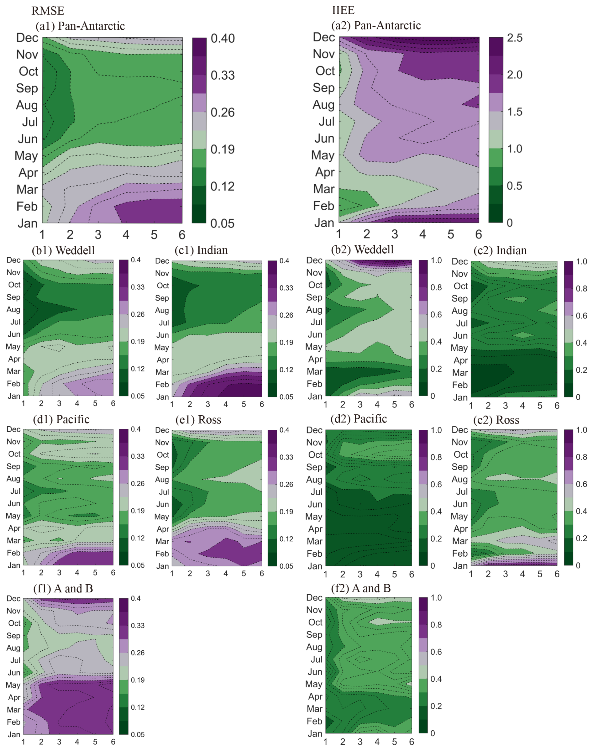
Figure 4 The predictive skill of sea ice concentration (spatially and temporally averaged during the testing years) in terms of RMSE and IIEE (units: million square kilometers) between the ANTSIC-UNet predictions and NSIDC observations for different target months and forecast lead times. “A and B” in (f1) and (f2) refer to the Amundsen Sea and Bellingshausen Sea, repsectively.

3.2 Predictive skill for interannual variability

We assess the performance of the predicted year-to-year variability of Pan-Antarctic and regional sea ice extent (SIE) anomalies (Fig. 5). For the Pan-Antarctic, the observed ice extent anomaly shifts from the positive phase to the negative phase around 2016 (Fig. 5a). The statistical and dynamical model cannot capture the observed shift after 2016, and the anomaly persistence model shows much larger positive anomalies and variability compared to the observation. SEAS5 struggles to capture the interannual variability of the Pan-Antarctic SIE, significantly overestimating anomalies in the Weddell Sea and Indian Ocean while underestimating anomalies in the Pacific Ocean. By contrast, ANTSIC-UNet reproduces the observed shift during 2014–2017 and the predicted interannual variability is well correlated with the observation (R=0.76). Moreover, the majority of the observed ice extent anomalies fall within the spread of the ANTSIC-UNet prediction, which is also true for most sub-regions (Fig. 5b–f). The highest correlation is found in the Weddell Sea (R=0.79), followed by the Indian Ocean (R=0.63) and Ross Sea (R=0.59). The Pacific Ocean, Amundsen and Bellingshausen Seas have relatively low correlations. Thus ANTSIC-UNet outperforms the statistical and dynamical models from the perspective of the SIE interannual variability prediction.

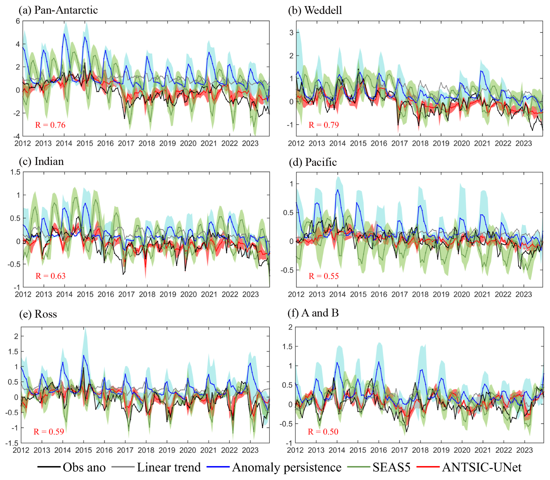
Figure 5 Sea ice extent anomalies from 2012 to 2023 (including both validation and testing years) for Pan- and regional Antarctic for NSIDC observations (black), the linear trend model (grey), the anomaly persistence model (blue), SEAS5 (green) and ANTSIC-UNet model (red). The shading represents the ensemble spread of anomaly persistence model (blue), SEAS5 (green) and ANTSIC-UNet (red) at different lead times up to 6 months, while the solid lines corresponding to the ensemble means. (units: million square kilometers).

Figure 6 further shows the evaluation metrics (ACC and MSSS) between the observed and predicted interannual sea ice extent. For the Pan-Antarctic, high values of ACC are found from January to September at 1–3 months lead, which decrease as the lead times increase (Fig. 6a). Reduced values of ACC are found from October to December as the lead time exceeds 2 months. MSSS exhibits a similar pattern as that of ACC (Fig. 6b). All sub-regions show similar distributions, high values of ACC and MSSS at 1-month lead and slowly decreasing with increasing lead times. Low values of ACC and MSSS occur in the Indian Ocean from Januray to March, the Pacific Ocean from November to January, and the Amundsen and Bellingshausen Seas from September to October, which limit the interannual predictive skill of the Pan-Antarctic. Overall, the Weddell and Ross Seas have broad coverage of high ACC and MSSS which suggests the possibility of long-lead extended seasonal predictions there.

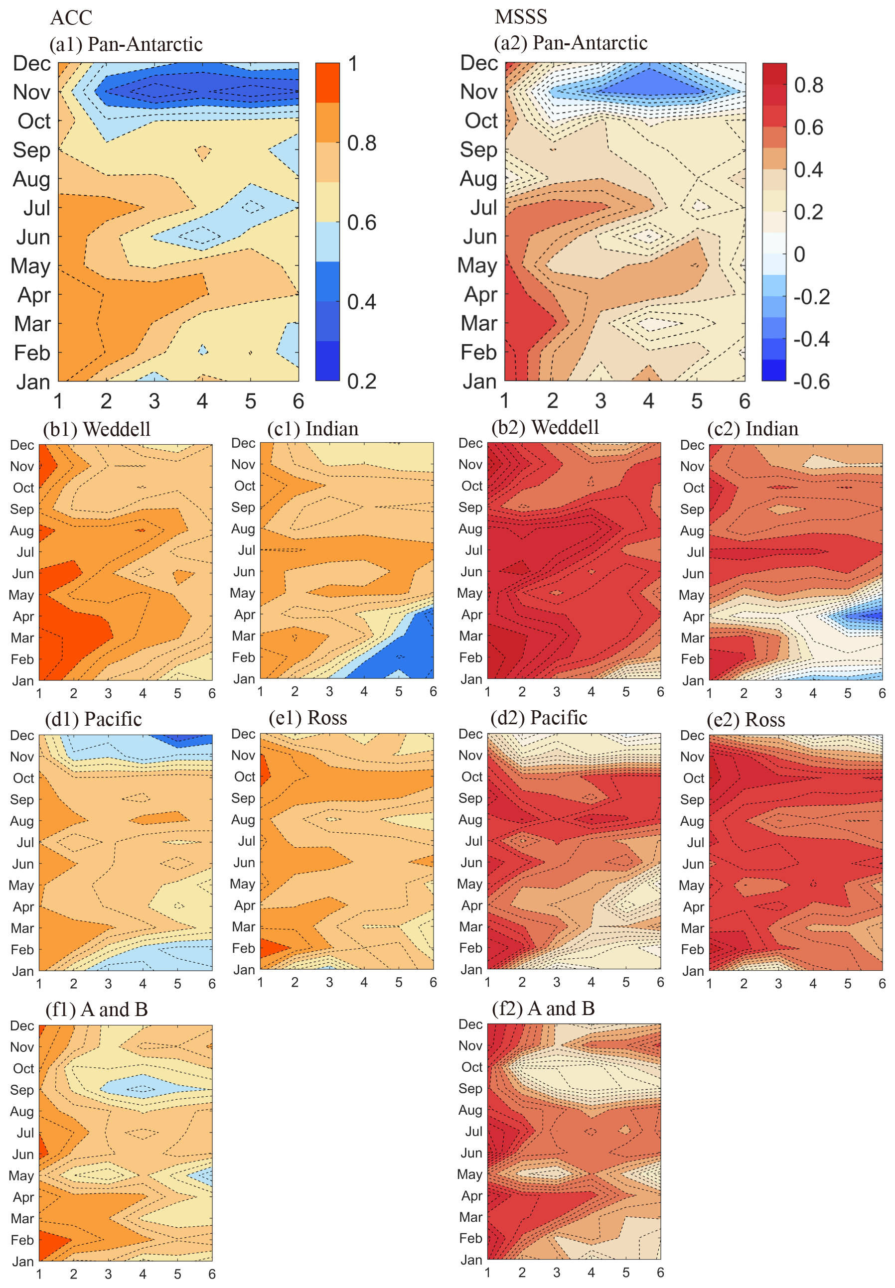
Figure 6 The ACC (a1–f1) and MSSS (a2–f2) between the observed and ANTSIC-UNet predicted regional SIE anomalies for different target months and forecast lead times during 1981–2023.

3.3 Extreme cases

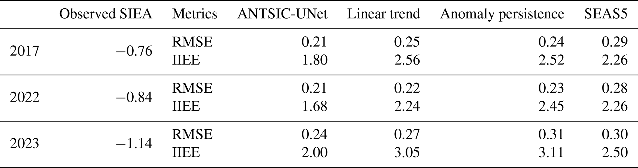
The past three extremely low Antarctic summer SIE events (Table 3) have been linked to key climate drivers and underlying mechanisms. For example, the anomalous sea ice melting during the summer of 2017 might be associated with early spring atmospheric conditions over the Southern Ocean being primarily influenced by a positive phase of the zonal wave 3 (ZW3) pattern, followed by a near-record negative Southern Annular Mode (SAM) (Turner et al., 2017; Schlosser et al., 2018). The significant weakening of the polar stratospheric vortex was identified as a key driver of the SAM changes (Wang et al., 2019). The extremely low sea ice events in the summer of 2022 and 2023 occurred with the deepening of the Amundsen Sea Low (ASL), triggering feedbacks that played a crucial role in the reduction of summer sea ice (Turner et al., 2022; Wang et al., 2022). A few studies have emphasized that the influence of a warm subsurface ocean is a contributor to the recent record-low summer sea ice events (Liu et al., 2023; Purich and Doddridge, 2023). Different large-scale atmospheric circulation patterns may also lead to similar regional prevailing winds, driving the negative Antarctic sea ice extent anomalies (Mezzina et al., 2024).

To our knowledge, little research has focused on the predictability of Antarctic sea ice extent in extreme years. Therefore, we evaluate to what extent the ANTSIC-UNet prediction can capture extreme years. The average predictive skills for the three extremely low sea ice extent years averaged for all lead times are shown in Table 3. During all extreme years, ANTSIC-UNet exhibits the smallest RMSEs and improves sea ice edge predictions with notably reduced IIEE, compared to the statistical and dynamical models. The spatial distribution of February and September SIC of 2023 (record low) is shown in Fig. 7. In February, the linear trend model overestimates sea ice concentration for much of the Antarctic. The anomaly persistence model shows clusters of large positive biases near the coastal area and extended northward coverage of negative biases at 1-month lead, and both magnitude and coverage of the biases increase dramatically as the lead time increases. SEAS5 underestimates SIC, and the negative biases increase with lead time, particularly in the Weddell Sea. ANTSIC-UNet exhibits better performance than the other models with smaller sea ice edge error for all lead times, though as lead time increases, the positive biases in the Amundsen and Ross Seas gradually increase. In September, the ANTSIC-UNet prediction shows smaller biases at sea ice edge in the entire Antarcic at 1-month lead compared to the other models, and still outperforms in most regions as the lead time increases. By comparison, SEAS5 shows substantial negative biases across the interior regions, in addition to significant biases at the sea ice edge. Though there are different spatial distributions of SIC errors for 2017 and 2022, ANTSIC-UNet also shows superior predictive skill (Figs. S1 and S2).

The models' predictive skill of seasonality errors of extremely low sea ice extent of 2023 are further accessed against the NSIDC observations (Fig. 8). Both the linear trend and anomaly persistence prediction models excessively overestimate the SIE in the Pan-Antarctic and all sub-regions for nearly all months, except for the Amundsen and Bellingshausen Seas. SEAS5 underestimates the SIE in the Pan-Antarctic and all sub-regions in summer. And it significantly overestimates the SIE during the sea ice expansion season, with positive biases in the Weddell Sea and Indian Ocean exceeding those of the linear trend model. In contrast, these positive SIE errors have been greatly reduced in the ANTSIC-UNet predictions. ANTSIC-UNet outperforms the linear trend model throughout the year for all the lead times and most regions, except for the Amundsen and Bellingshausen Seas. This is also true for 2017 and 2022 (Figs. S3 and S4). Therefore, ANTSIC-UNet has excellent predictive skills for extreme events in recent years.

Table 3 The averaged predictive skill of ANTSIC-UNet, statistical models (linear trend and anomaly persistence models) and SEAS5 for the extreme summer years of Antarctic sea ice. Here, observed SIEA represents February monthly anomalies of sea ice extent from NSIDC observations for these extreme years, calculated by subtracting the February average sea ice extent for the period 1981–2011 (units: million square kilometers). RMSE: root-mean-square error; IIEE: integrated ice-edge error.

We further compared the ANTSIC-UNet's accuracy performance on sea ice edge predictions for the extreme summer years, relative to linear trend predictions and SEAS5. As shown in Fig. 9, both ANTSIC-UNet and SEAS5 have increasing sea ice edge errors as lead time increases. Note again that the linear trend predictions are independent of lead time. ANTSIC-UNet outperforms SEAS5 and linear trend predictions at sea ice edge error in all extreme summer years. At short lead times, ANTSIC-UNet has substantial improvement relative to the linear trend predictions and moderate improvement compared to SEAS5. At long lead times, ANTSIC-UNet's improvements relative to SEAS5 become more significant. These results suggest that ANTSIC-UNet has high predictive skills for extended seasonal predictions of Antarctic sea ice concentration, especially for extreme events, compared to other statistical and dynamical models.

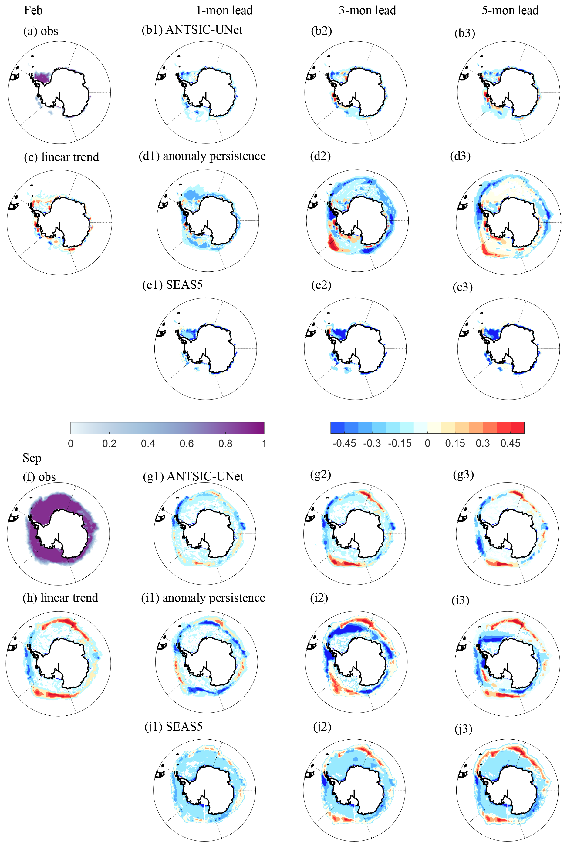
Figure 7 February and September 2023 SIC of NSIDC observations (a, e) and errors predicted by ANTSIC-UNet (b1–b3, g1–g3), the linear trend model (c, h), anomaly persistence model (d1–d3, i1–i3) and SEAS5 (e1–e3, j1–j3) at lead time of 1, 3 and 5 months (lowest sea ice extent on record).

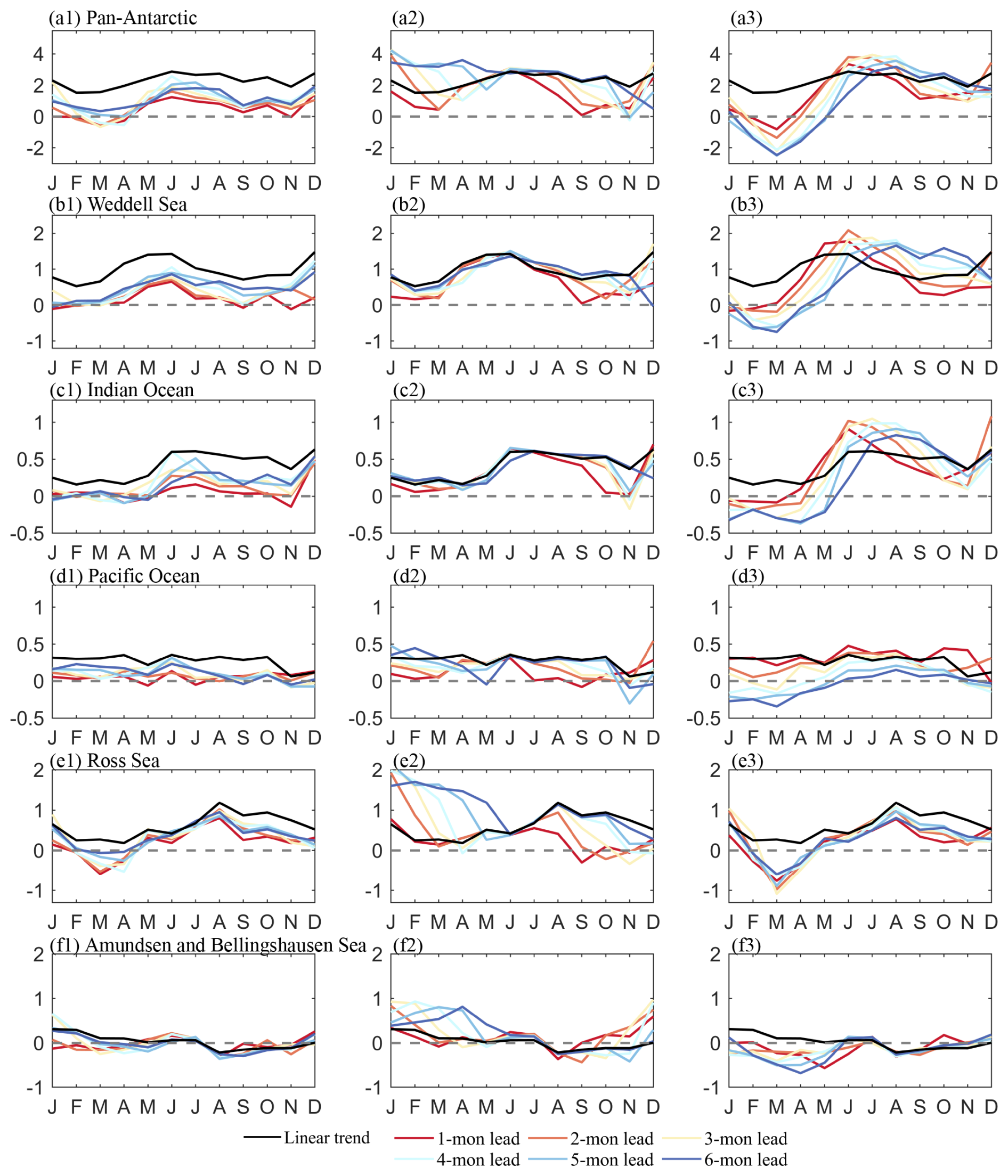
Figure 8 Seasonality errors of the Pan- and regional Antarctic monthly mean SIE (SIC > 15 %) between NSIDC observations and ANTSIC-UNet (a1–f1), anomaly persistence model (a2–f2) and SEAS5 (a3–f3) predictions at different lead times for 2023 (lowest sea ice extent on record in Feburary). The black lines show the seasonality SIE errors between observations and linear trend model. (units: million square kilometers).

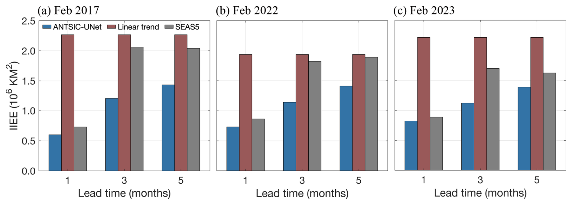
Figure 9 Integrated ice-edge error (IIEE) of ANTSIC-UNet, the linear trend forecast and SEAS5 for February forecasts at lead time of 1, 3, and 5 months for the extreme summer years. (a) 2017, (b) 2022 and (c) 2023.

3.4 Variable importance

In this study, 14 atmospheric and oceanic variables from ERA5 and ORAS5 are selected to capture the key physical mechanisms influencing sea ice variation. Variables such as sea surface temperature, 2 m air temperature, and radiation impact heat flux exchanges at the air-ice-sea interface (Bourassa et al., 2013). Near surface winds drive sea ice movement and large-scale tropospheric circulation impacts sea ice through its effects on winds, temperature, precipitation, and cloud cover (Raphael and Hobbs, 2014). The 10 hPa zonal wind represents stratospheric zonal circulation, which impacts surface circulation through downward propagation, influencing sea ice dynamics (Cordero et al., 2023). Sea temperature anomalies and the upper-ocean heat content anomaly for the upper 300 m taken from ORAS5 play a crucial role in the heat energy exchange at the ocean–ice interface (Purich and Doddridge, 2023; Bianco et al., 2024). The upwelling of warmer subsurface water can further influence sea ice formation and melting in the high latitude of the Southern Ocean (Cai et al., 2023). As discussed, ANTSIC-UNet shows better performance compared to the linear trend and anomaly persistence models. This implies that ANTSIC-UNet has learned to predict extended seasonal Antarctic sea ice based on the physical relationships of the input variables.

Previous studies suggested that the evaluation metrics of model's predictive skill, especially for models with strong generalization ability, correlate closely with feature importance (FI) (Andersson et al., 2021; Molnar, 2019). The permutation feature importance method based on testing variables can reveal the model-dependence variables and indicate the contribution extent of the variables to the performance of the model on unseen data. Here we use the permutation feature-importance method to explain model variance based on the testing data from 2020–2023. The variable importance is Pan-Antarctic averaged for all calendar months (Fig. 10), and indicates that ANTSIC-UNet is gaining skills from some important variables, including sea ice conditions, sea surface temperature, radiative flux, and stratospheric wind. ANTSIC-UNet also ignores some peripheral variables, such as sea level pressure and subsurface ocean temperature. At short lead times, on timescales of up to two months, ANTSIC-UNet relies more on the initial sea ice state and linear trend prediction, as well as the surface upward shortwave radiation, sea surface temperature, atmospheric conditions in the troposphere, and 10 hPa zonal wind in the stratosphere. This implies that ANTSIC-UNet has learned the dynamic and thermodynamic physical mechanisms directly forcing sea ice variations (Son et al., 2009; Turner et al., 2016). At longer lead times, in addition to historical SIC conditions and linear trend predictions of SIC at the target month, the 10 hPa zonal wind stands out as an important influencing factor which manifests the lagged response in Antarctic sea ice to changes in stratospheric circulation (Raphael and Hobbs, 2014; Wang et al., 2021).

When a variable shows minimal or even negative importance, it suggests that the ANTSIC-UNet might be overlooking that feature or has not yet fully captured the intrinsic relationships involving that variable. It may also be related to the accuracy of the reanalysis data used as input. For example, the lack of predictive importance for downward solar radiation could be due to this variable being poorly represented in the Southern Ocean within the reanalysis as discussed above. Thus, it is crucial to consider the accuracy of input variables chosen from reanalysis data for Antarctic sea ice predictions.

3.5 Phyical constraints

The ANTSIC-UNet model is trained based on minimizing the loss function which measures the difference between the output and the desired targets. We optimize ANTSIC-UNet using the mean square error (MSE) of SIC as its original loss function. However, the pronounced prediction errors often occur in the vicinity of the sea ice edge, likely associated with oceanic influence and wind dynamics. Interestingly, Ren and Li (2023) suggested that the normalized integrated ice-edge error loss might be suitable for long sequence SIC predictions. The question is whether a physically constrained loss function in deep learning models can improve the extended seasonal forecast of Antarctic sea ice. Here we test a hybrid loss function combining MSE and IIEE to optimize spatial predictions and minimize sea ice edge errors. IIEE loss is calculated by dividing the difference between the predicted and observed sea ice extent by the sum of SIE where SIC > 0.15 % in both the prediction and observation. We assign a weight of 0.05 to the IIEE components for values balance in the hybrid loss expression (Eq. 10). Hence, the two loss functions are calculated as:

$$\begin{array}{}\text{(9)}& {\displaystyle }\text{Original Loss}=\text{MSE}=\text{mean}(\sum (p-o{)}^{\mathrm{2}}),\text{(10)}& {\displaystyle }\text{Hybrid Loss}=\text{MSE}+\mathrm{0.05}{\displaystyle \frac{\mathrm{IIEE}}{{\mathrm{SIE}}_p\cup {\mathrm{SIE}}_o}},\end{array}$$

where p (SIE_p) is the predicted sea ice concentration (ice extent) by ANTSIC-UNet and o (SIE_o) is the observed ice concentration (ice extent). For clarity, we denote the original loss (hybrid loss) as subscripts “o” (“h”) for distinguish between the ANTSIC-UNet models trained with two different loss functions.

Our results show similar distributions of sea ice edge errors predicted by two ANTSIC-UNet models (Figs. 4a2–f2 and 11a1–f1) with small values of IIEE at 1-month lead and large values from November to January as the lead time exceeds 2–4 months. ANTSIC-UNet_h trained with the hybrid loss slightly reduces the IIEE for the Pan-Antarctic compared to ANTSIC-UNet_o, especially in Weddell Ocean, Ross Amundsen and Bellingshausen Seas (∼ 0.02–0.05 million km²).However increased errors occur in these regions as lead time exceeds 3–4 months (Fig. 11a2–f2).

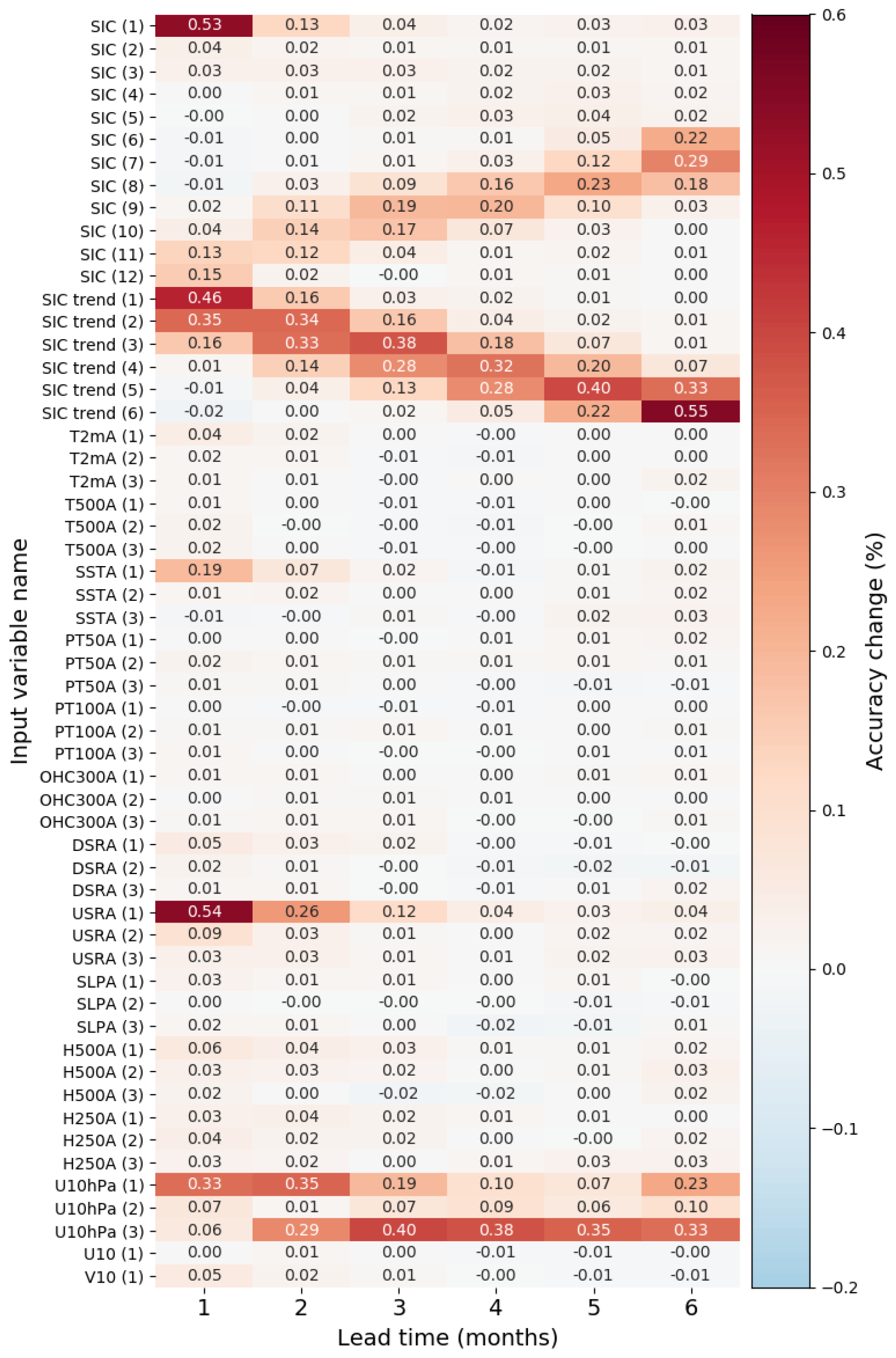
Figure 10 The results of variable importance analysis for Pan-Antarctic based on the permutation feature importance measurement (see Table 1 for full name of the variables).

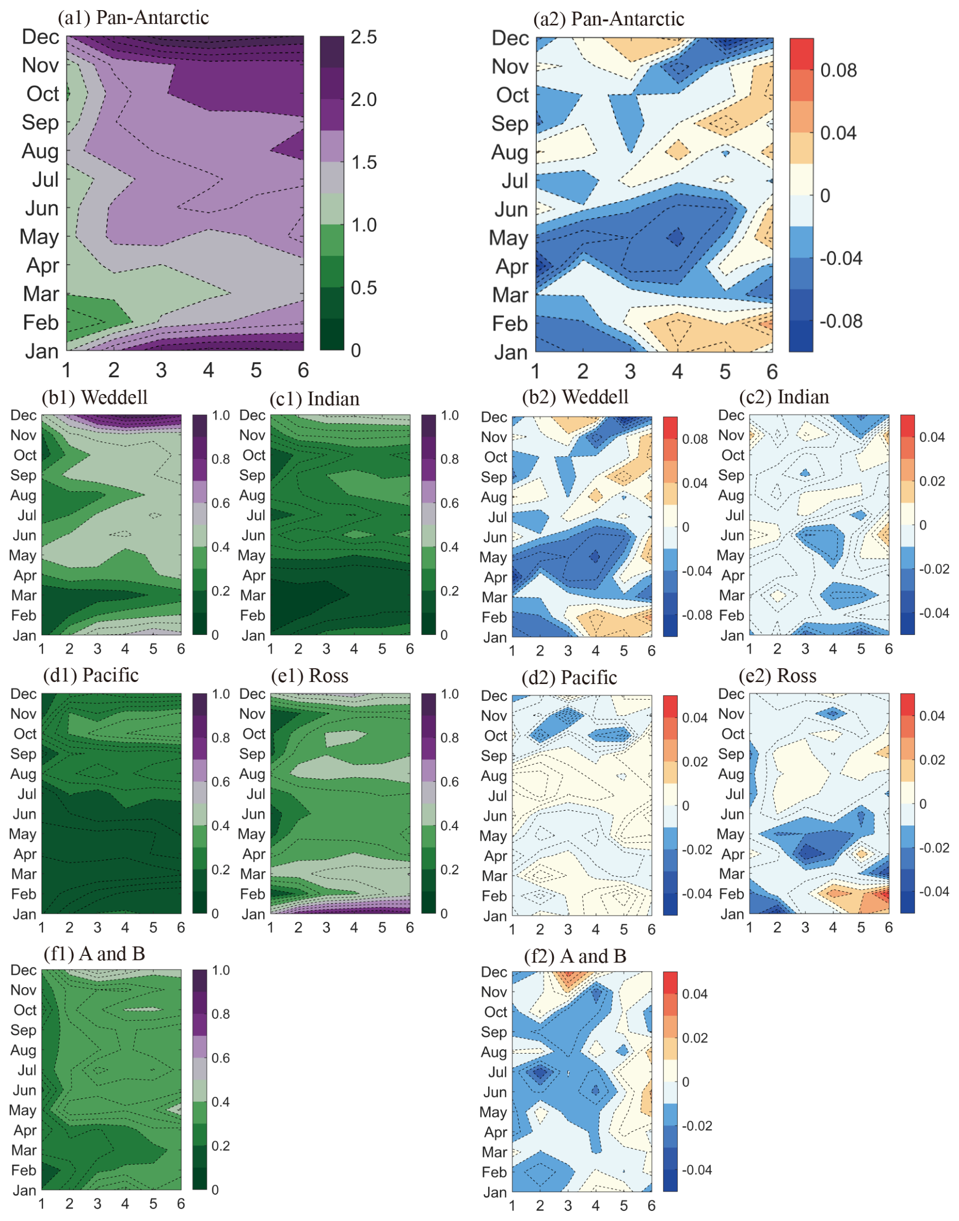
Figure 11 The IIEE of ANTSIC-UNet_h (a1–f1) and difference (b2–f2) between the two ANTSIC-UNet models trained with different loss functions for different target months and forecast lead times spatially and temporally averaged during the testing years (units: million square kilometers).

4 Discussion and conclusion

Antarctic sea ice extent exhibits significant variability driven by the complex air-ice-sea interactions that are not yet fully understood. Sea ice concentration is the essential variable for investigating the variation of sea ice (i.e., extent) and the satellite observations provide long-term reliable records of the data since the late 1970s. However, the accurate prediction of Antarctic sea ice, especially for extended seasonal timescales, remains a challenge due to the difficulty in fully capturing these complex interactions within existing models. In addition, there has been limited focus on systematic evaluation of model performance during extreme years. In this study, we have introduced a deep learning model, ANTSIC-UNet, to predict the extended seasonal Antarctic monthly-mean sea ice concentration. Considering the complex physical processes influencing Antarctic sea ice variability, atmospheric and oceanic variables, in addition to sea ice itself, are used for ANTSIC-UNet's forecasts. We compare the deep learning predictions against statistical models (the linear trend and anomaly persistence models) and a dynamical model (SEAS5), to evaluate the predictive skill of both Pan- and regional Antarctic sea ice. ANTSIC-UNet exhibits superior predictive skill for Antarctic sea ice for at least 6 months lead, and provides particularly improved predictions of extreme low sea ice events in recent years. The prediction performance of ANTSIC-UNet shows pronounced seasonality and regional dependence, which affects the predictive skill of the Pan-Antarctic. Specifically, during the autumn to spring, low RMSE is observed for most sub-regions. However, increased RMSE is evident in summer for lead time exceeding 2 months indicating decreased model performance in that season. Small values of integrated ice-edge error (IIEE) are found in summer at 1–3 months lead, but large errors occur from November to January as the lead time exceeds 2–4 months. Low RMSE and broader coverage of small IIEE suggest superior predictive skills in the Pacific and Indian Oceans at the sea ice edge zone in summer. Our findings are consistent with those of Marchi et al. (2019) and Bushuk et al. (2021) that sea ice concentration prediction tends to be more accurate in the winter months but less so in the summer due to rapid and irregular changes in the ice edge during that season. Inspiringly, ANTSIC-UNet shows lower summer sea ice edge error and SIC RMSE compared to both the two benchmark models and the dynamical model, especially during extreme years. The differences in model performance across regions could be attributed to regional variability due to oceanographic conditions, sea ice dynamics, and the influence of atmospheric and oceanic circulation patterns. Regional seas in the West Antarctic, including the Ross Sea, Amundsen Sea, Bellingshausen Sea, and Weddell Sea, exhibit larger interannual variability in sea ice concentration compared to the East Antarctic (Cavalieri and Parkinson, 2008). These regions are influenced by the Circumpolar Deep Water (CDW), with warm-shelf regions such as the Amundsen and Bellingshausen Seas being particularly sensitive to climate changes, with sea ice concentration and the position of the ice edge strongly driven by wind forcing (Stammerjohn et al., 2003; Saenz et al., 2023). The ice flux driven by wind in the Weddell Sea along the Antarctic Peninsula and the Pacific Ocean plays a crucial role in modulating sea ice dynamics, with the dynamical influence being more pronounced in the Pacific sector (Holland and Kwok, 2012). The sea ice increase (decrease) in the Ross Sea (Bellingshausen Sea) is linked to the Amundsen Sea Low (ASL) which is a key climate feature of these regions (Hosking et al., 2013; Turner et al., 2016). In contrast to other regions of Antarctica, sea ice expansion in the Indian Ocean sector is significant throughout all seasons and is associated with surface cooling and ocean renewal processes that stabilize the ocean and limit the intrusion of warmer subsurface waters into the surface layer (Bintanja et al., 2013; Purich et al., 2018). Additionally, seasonal variability in sea ice in the Indian Ocean sector is closely linked to the Southern Annular Mode (SAM) (Yadav et al., 2022).

We further assess the prediction performance for year-to-year variability: ANTSIC-UNet shows good predictive skill in capturing the interannual variability of Pan-Antarctic and regional sea ice extent anomalies. Consistently high values of ACC and MSSS, as revealed for the Weddell and Ross Seas, encouragingly suggest the possibility of performing long-lead extended seasonal predictions. Moreover, the results from the variable importance analysis, computed by a post-hoc interpretation method, suggest that ANTSIC-UNet has learned the important relationship between the sea ice and other climate variables having varying impacts across different lead times. Specifically, at short lead times, ANTSIC-UNet predictions are sensitive to initial conditions and linear trend predictions of SIC, sea surface temperature, radiative flux and vertical atmospheric circulation conditions. At longer lead times, predictions are dependent on historical conditions and linear trend predictions of SIC, and stratospheric circulation patterns. The issue that Amundsen and Bellingshausen Seas have the lowest predictive skill might be associated with ANTSIC-UNet ignoring the sea level pressure and hence the tropical teleconnection relationship associated with the strengthening of Amundsen Sea Low (ASL) in recent decades (Li et al., 2021; Cai et al., 2023). Our feature importance findings can be associated with recent work by Uebbing et al. (2025) investigating the impact of feature reduction on seasonal Arctic sea ice forecasting by using the state-of-the-art IceNet model (Andersson et al., 2021) combined with explainable AI (XAI) techniques. Their study showed that using only a subset of key features (such as historical sea ice concentration, linear trend forecasts, and seasonal encoding), high predictive accuracy under general scenarios was still obtained. However, their research also highlighted that for extreme events, such as anomalous sea ice extents, models incorporating additional climate variables perform better. This suggests that further studies might benefit from exploring different XAI methods for estimating feature importance and investigating the extent to which the reduction of the number of features affects deep learning model predictions for Antarctic sea ice.

Finally, our findings suggest that incorporating physical constraints into ANTSIC-UNet could further improve the model's performance at the sea ice edge of the Pan-Antarctic for extended seasonal predictions. Thus ANTSIC-UNet provides a useful tool for extended seasonal prediction of Antarctic sea ice concentration and extent, and for analyzing physical processes important for sea ice variations in different regions. The results from variable importance analysis show evidence that ANTSIC-UNet successfully extracts key information from the complex ocean-ice-atmosphere interactions to predict sea ice concentration and capture seasonal variations through different climate variables. This approach could be effectively extended to other sea ice variables once the relevant long-term data becomes available (i.e., sea ice thickness). Existing data on Antarctic sea ice thickness, derived from satellite altimetry missions including the ICESat data (from 2003–2008), ICESat-2 data (from late 2018 onward) and CryoSat-2 data (from 2010 onward) remain limited in terms of confidence and temporal coverage and yet are not suitable for direct deep learning applications (Hendricks et al., 2018; Kacimi and Kwok, 2020; Fons et al., 2023). Additional efforts are needed for refining and integrating these datasets into predictive models. The Polar Pathfinder product (Tschudi et al. 2019) provides daily sea ice motion vectors at a spatial resolution of 25 km, which are valuable for investigating sea ice movement patterns under the influence of wind and ocean currents. Future research will explore whether incorporating dynamic factors such as ice drift can enhance the accuracy of sea ice predictions. An important direction for future work will be to systematically compare model forecast performance across different Antarctic regions and during extreme events, using alternative ML approaches, including generative models. In addition, further investigation based on physically enriched deep learning models is also needed to explore more thoroughly the physical mechanisms between SIC and other climate variables with long-term memory, such as sea ice thickness and ocean heat content (Marchi et al., 2019; Bushuk et al., 2021; Libera et al., 2022).