Multitemporal analysis of Sentinel-1 backscatter during snowmelt using high-resolution field measurements and radiative transfer modelling

The spatiotemporal evolution of snowmelt is fundamental for water resources management and risk mitigation in mountain catchments. Synthetic aperture radar (SAR) images acquired by satellite systems such as Sentinel-1 (S1) are promising for monitoring wet snow due to their high sensitivity to liquid water content (LWC) and ability to provide spatially distributed data at a high temporal resolution. While recent studies have linked multitemporal S1 backscatter to snowmelt phases, a correlation with detailed snowpack properties is still missing. To address this, we collected the first dataset of comprehensive wet-snow properties tailored for SAR applications over two consecutive snow seasons at the Weissfluhjoch field site near Davos, Switzerland. First, we tested previous methods which use multitemporal S1 backscatter to characterize melting phases and demonstrated that the observed monotonous increase in backscatter following the local minimum is due to the development of surface roughness. Then, we used the measured snow properties as input to the Snow Microwave Radiative Transfer (SMRT) model to reproduce S1 backscatter signals. Our simulations showed that rather than melting phases, time series of backscatter identify regimes dominated by either LWC, early in the season, or surface roughness, later on. The results also highlight several key challenges for reconciling S1 signals with radiative transfer simulations of wet snow: (i) the discrepancy in spatiotemporal variability of LWC as seen by the satellite and validation measurements, (ii) the lack of fully validated permittivity, microstructure and roughness models for wet snow in the C-band, and (iii) the difficulty of capturing wet-snow features potentially generating stronger scattering effects on a large scale – such as internal snowpack structures, soil features in case of low LWC and surface roughness – which are not necessarily captured by pointwise measurements.

1 Introduction

Seasonal snowpack in mountain catchments is one of the most important water resources, as it accumulates and stores water during winter and releases it consistently in the form of runoff during the melting period (Viviroli and Weingartner, 2004). In alpine streams, discharge is largely dominated by snowmelt from May to July, and more than one-sixth of the world's population relies on meltwater released from higher altitudes for drinking water, crop irrigation and hydropower production (Beniston et al., 2018). However, melting snow can also cause wet- and glide-snow avalanches (Bellaire et al., 2017; Fromm et al., 2018), which pose significant threats to human life and infrastructures. Additionally, rain-on-snow events on already wet snowpacks are linked to increased runoff and shorter time lags between precipitation onset and the resulting runoff (Würzer et al., 2016). These events can have catastrophic consequences, and their occurrence is supposed to increase in response to sustained warming (Beniston and Stoffel, 2016). Therefore, information about the spatiotemporal evolution of snowmelt is beneficial for both the management of water resources and risk mitigation.

Identifying wet snow is complex when using both manual measurements or automatic instruments and physics-based snow models. Datasets of manual measurements of snow water equivalent (SWE) and liquid water content (LWC hereafter) at high temporal resolution are generally rare due to the time, effort and resources required for their collection. There have been considerable advances in technologies that use the dielectric properties of snow in the microwave range to estimate LWC in a non-destructive way (Schmid et al., 2014; Koch et al., 2014). However, the application of these methods is limited to one single point without the possibility of capturing the spatial variability of the processes. Additionally, their installation and maintenance are often complicated and expensive, and the extraction of the physical parameters is usually hindered by noise. Physics-based layered snow models like the SNOWPACK–Alpine3D model chain (Bartelt and Lehning, 2002; Lehning et al., 2006) or GEOtop (Endrizzi et al., 2014) are used to overcome these challenges, as they can simulate LWC and SWE at high spatial and temporal resolutions based on meteorological forcings. However, meteorological forcings also represent a major source of uncertainty – especially when needed at high spatial resolution – affecting the accuracy of the results (Raleigh et al., 2015). This is in addition to the uncertainties related to the number and type of parametrizations used (Günther et al., 2019).

In this context, a valuable opportunity to identify wet snow is offered by synthetic aperture radar (SAR hereafter) systems. SAR measurements are highly sensitive to the free liquid water contained in wet snow (Nagler and Rott, 2000). At certain frequencies, the increase in liquid water generates high dielectric losses and increased absorption coefficients (Denoth et al., 1984; Sihvola and Tiuri, 1986; Mätzler, 1987; Ulaby et al., 2014). Therefore, the radar backscatter drops to lower intensities with respect to winter averages (Ulaby et al., 1987; Strozzi et al., 1997; Strozzi and Matzler, 1998; Nagler and Rott, 2000; Ulaby et al., 2014; Nagler et al., 2016; Lin et al., 2016). This raises the question of whether different types of snow cover could be classified based on their response to active microwave signals. This challenge has been addressed with various approaches over the years. Between 1993 and 1995, at the field site of Weissfluhjoch in the Swiss Alps, Strozzi et al. (1997) and Strozzi and Matzler (1998) conducted tower-based C-band radiometric measurements at all polarizations across a wide range of incidence angles. Simultaneously, they carried out monthly measurements of snow physical properties. These measurements were used to classify the observed snow cover types into categories ranging from dry snowpacks to thin moist layers overlying dry snow to wet snowpacks with either smooth or rough surfaces. Relying on a tower-based radiometer, the experiments were highly controlled, allowing detailed investigation of radar responses to each snow condition. Nevertheless, significant sources of uncertainty remained – especially the influence of surface roughness on wet-snow surfaces, which was not quantitatively measured but only qualitatively assessed. These detailed studies, along with the work of Kendra et al. (1998), raised questions about the theoretical foundations and systematic reliability of LWC retrieval algorithms based on C-band fully polarimetric SAR imagery, which had been developed shortly before (Shi et al., 1993; Shi and Dozier, 1995). In particular, the scattering mechanisms assumed in these retrievals may have been biased by a combination of conditions that strongly favoured surface scattering. Extending the prior knowledge to a spatial and multitemporal context, Nagler and Rott (2000) developed an algorithm based on repeat-pass SAR images to map wet snow in mountainous areas, defining a backscatter drop of 3 dB to distinguish wet snow from other surfaces. Comparisons with snow maps from different sources showed generally good agreement above the snow line but consistent biases in areas with fragmented snow cover.

After a progress freeze due to the scarcity of SAR data in past and simultaneous field measurements, research interest in the topic was renewed after the launch of the Sentinel-1 (S1 hereafter) joint mission of the European Space Agency (ESA) and the European Commission in 2014. At alpine latitudes, S1 acquires C-band SAR imagery in the early morning and late afternoon, regardless of the weather, with a revisit time of 6 calendar days. The SAR imagery is available free of charge. Marin et al. (2020) used these images for the first time to develop a correlation between the multitemporal S1 SAR backscatter and the snowmelt dynamics. Over 5 different alpine sites, the authors found that the multitemporal S1 SAR acquisitions allow the detection of the melting phases, i.e. moistening, ripening and runoff (Dingman, 2015), with good agreement with in situ observations and layered, physics-based snow models. In particular, the backscatter decreased as soon as liquid water appeared in the snowpack and increased progressively and simultaneously with the runoff release. Deriving and applying a set of identification rules, the authors could define the melting phases for the test sites with relatively small lag errors with respect to the revisit time of S1. Consequently, local minima in S1 multitemporal backscatter time series and sharp increases thereafter were associated with snowpack saturation, the onset of runoff and snow ablation (Darychuk et al., 2023; Gagliano et al., 2023).

These approaches hold great potential for monitoring the temporal evolution of the melting dynamics, particularly over wide and scarcely instrumented areas. However, to fully use the multitemporal information provided by S1 for snowmelt monitoring, a deeper understanding of the underlying scattering mechanisms – especially the role of surface roughness (Marin et al., 2020) – is still required. Specifically, knowing the time window in which different scattering effects dominate and under which conditions the C-band radar backscatter is fully absorbed by the melting snowpack would enable us to extract as much information as possible from S1 time series. To date, the only effort in this direction has been made by Brangers et al. (2024) using tower-based C-band measurements. However, this study lacks high-temporal-resolution ground-truth validation with measured snow properties. Moreover, comparisons with S1 were hindered by several factors, including sensor calibration issues and the small footprint size – which likely introduced speckle noise, and they failed to capture larger-scale scattering processes.

Overall, the main limitation to improving the understanding of the interaction of S1 backscatter signals with melting snow cover is the lack of reference ground data. Over alpine snowpacks, it is common to observe the formation of ice layers either at the surface (Quéno et al., 2018) or at deeper snowpack depths (Pfeffer and Humphrey, 1998). Moreover, in temperate alpine areas characterized by high snow accumulation and intense solar radiation, suncups may form spontaneously on the snow surface during the ablation season (Post and LaChapelle, 2000; Mitchell and Tiedje, 2010), increasing the surface roughness significantly (Fassnacht et al., 2009). These phenomena are known to impact the radar response to wet snow (Shi and Dozier, 1995; Strozzi and Matzler, 1998; Kendra et al., 1998; Nagler and Rott, 2000; Yueh et al., 2009).

However, high-resolution and detailed snow measurements alone are insufficient to address this issue. It is equally important to rely on a method to interpret them from a radar perspective. A promising and increasingly adopted approach involves the use of state-of-the-art radiative transfer (RT hereafter) models. Picard et al. (2018) developed the Snow Microwave Radiative Transfer (SMRT) model, a versatile model that can be used in active and passive mode to compute backscatter and brightness temperature from multilayered media such as snowpacks or ice sheets overlying reflective surfaces, e.g. ground, ice, or water. SMRT responds to the need of a modular and flexible approach to unify and compare the wide range of pre-existing representations of microstructure, electromagnetic theories, soil models and permittivity formulations. While wet snow holds significant importance for various applications, both SMRT and other similar models were primarily developed and validated for dry snow conditions in Arctic and Antarctic snowpacks or ice sheets (Proksch et al., 2015; Rott et al., 2021; Soriot et al., 2022; Meloche et al., 2022; Husman et al., 2023). Both the vertical structure and the surface of these types of snowpack are often less complex than those of a seasonal alpine snowpack. To date, the above-mentioned ensemble of complex melting snowpack processes has scarcely been investigated by means of radiative transfer models due to the lack of ground reference data (Shi and Dozier, 1995; Strozzi et al., 1997; Kendra et al., 1998; Nagler and Rott, 2000; Magagi and Bernier, 2003; Lodigiani et al., 2025). Murfitt et al. (2024) recently used SMRT to explore, for the first time, the temporal evolution of the interaction between wet snow and radar waves in a study on lake ice melt. However, the radiative transfer modelling of wet snow still lacks dedicated effort and validation.

The objective of this work is to collect the first ground reference dataset on melting snow tailored for SAR applications and to use it together with SMRT to better understand the key processes governing the backscatter signatures recorded by S1. Previously, only Lund et al. (2022) had carried out a similarly extensive snow pit campaign in coordination with S1 passages. While this study helped advance the interpretation of S1 backscatter responses to diurnal snowpack variations, important scattering properties such as the optical diameter and the surface roughness were not measured. As a result, interpreting these measurements from the radar perspective – and consequently comparing them with S1 acquisitions – was not possible. In our work, we focus on the co-polarized vertical backscattering only, due to its high signal-to-noise ratio for wet snow (Naderpour et al., 2022) and to the fact that, because of the partial implementation of some of the key processes, it is not possible to simulate accurate cross-polarized backscattering responses with the current version of SMRT. To our knowledge, this is the first attempt to translate ground measurements – specifically designed for RT modelling, including wetness and roughness – into radar signals using SMRT to reproduce and interpret S1 acquisitions over a wet, multilayered alpine snowpack. This research provides valuable insights in two main areas. First, it advances the understanding of the interaction between S1 radar backscatter and wet snow. Specifically, it reveals the effects of spatiotemporal variability of LWC within the S1 footprint occurring between satellite and measurement acquisitions. It also describes the impact of surface roughness on backscatter signatures and highlights challenges in capturing key wet snow conditions that likely generate scattering at wider scales. These include internal snowpack structures, large-scale surface roughness and interactions with the wet-soil interface when the snowpack is only slightly wet. Second, the study addresses the RT modelling of melting, layered snowpacks, highlighting the current lack of fully validated permittivity and roughness models for wet snow at C-band frequencies. With ground reference data and adequate process understanding and modelling, RT models like SMRT may evolve in terms of tools to interpret the information contained in multitemporal SAR backscatter and translate it into valuable input for snow-hydrological modelling.

2 Campaign overview

This work builds upon a dataset of 85 snow pits collected during a two-season campaign (2022–2023 and 2023–2024) at the high-altitude Weissfluhjoch Versuchsfeld (WFJ) field site, located in the Rhaetian Alps near Davos, Switzerland. The measurement field lies at an altitude of 2536 m a.s.l. on a relatively flat area embedded in a south-east-facing valley. The site is partially wind sheltered by a small hill situated to the south-east – however, the dominant wind blows from the north-west, in addition to katabatic wind. For this measurement campaign, we secured a protected field covering approximately 2 times the footprint area of S1, i.e. 20×20 m. However, only a portion of this field was effectively used for measurements, while the remaining area was consistently left undisturbed. The secured field has a light-slope value of between 2 % and 7 %. The flatness of the terrain is fundamental for the study of the interaction between wet snow and the C-band co-polarized vertical backscatter signal (${\mathit{\sigma }}_{\mathrm{0}}^{\mathrm{VV}}$ hereafter). On the one hand, ${\mathit{\sigma }}_{\mathrm{0}}^{\mathrm{VV}}$ is less sensitive to changes in snow wetness at low incidence angles (Nagler et al., 2016); on the other hand, on steep slopes, the liquid water is redistributed laterally, at least partially (Wever et al., 2016). The field site of WFJ is equipped with advanced meteorological sensors recording meteorological forcings at sub-hourly resolutions, and moreover, with the first snow observations dating back to 1936, it holds one of the longest recorded time series of snow measurements for a high-altitude research station (Marty and Meister, 2012). The site is ideal for intensive measurement campaigns, as it is easily accessible and protected from avalanche danger and the two huts provide shelter, storage space for instruments, power and an internet connection.

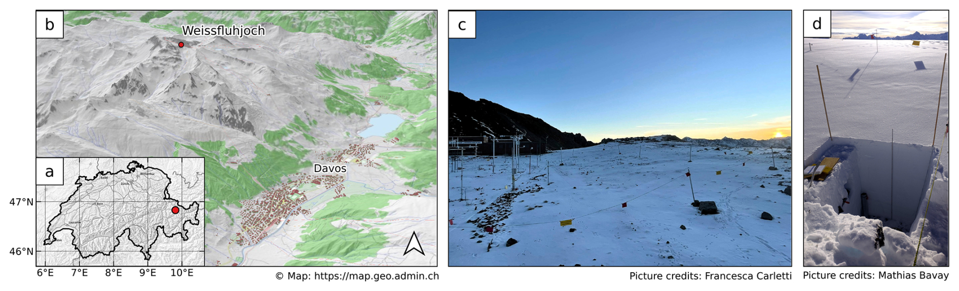
Figure 1 Location of the Weissfluhjoch field site with respect to Swiss national borders (a) and the town of Davos (b). The designated area for snow profiles is shown in (c) under semi-snow-free conditions (picture taken in September 2024, camera oriented towards the north-east), enclosed by a flagged fence. It is worth noting that only a portion of this fenced area was effectively used for snow profiles. Panel (d) shows the typical snow pit measurement setup.

The objective of the measurement campaign was to build a dataset of ground-truth reference for the interpretation of S1 ${\mathit{\sigma }}_{\mathrm{0}}^{\mathrm{VV}}$ to monitor snowmelt processes. Therefore, the measurements targeted the main scattering properties of snow: temperature, density, specific surface area (SSA), liquid water content (LWC) and surface roughness. These properties needed to be measured at a high vertical and temporal resolution to track the progression of the wetting front within the snowpack and possibly concomitantly with S1 acquisitions. Additionally, we measured snow water equivalent (SWE), a key variable for snowmelt monitoring. The resulting dataset is a time series of manually measured snow profiles describing the evolution of snow scattering properties at unprecedented vertical and temporal resolutions. The dataset consists of 38 snow profiles for the season of 2022–2023 (starting in February and ending in June) and 47 for the season of 2023–2024 (starting in November and ending in July). In dry snow conditions, measurements were carried out once per week. In the first season, once the snowpack reached the full isothermal state, measurements were carried out regularly every second working day for a total of three times per week. In the following season, the regularity of the measurements was partially given up in favour of better synchronization with S1 acquisitions. To get the fullest possible picture to interpret the melt dynamics, manual measurements are accompanied by automatically recorded time series of runoff and SWE.

2.1 Manual measurements

2.1.1 Temperature

Snow temperature serves to monitor the progression of the snowpack to the isothermal state, which allows the presence of liquid water. Profiles of snow temperature were sampled from the surface to the bottom with a vertical resolution of 10 cm in snow season 2022–2023 and of 5 cm in snow season 2023–2024 using a batch of HI98501 Checktemp instruments from Hanna (, ). According to the instrument specifications, the uncertainty range is ±0.2 °C. Each temperature reading was marked down after waiting for an adequate amount of time for measurement stabilization.

2.1.2 Density

In dry snow conditions, snow density controls (i) the probability of scattering events, as denser snow has more grains per unit volume, and (ii) the real part of the effective permittivity (see Sect. 3.2), which increases with the increased fraction of ice relative to air, typical of denser snow. Profiles of snow density were sampled from the surface to the bottom with a vertical resolution of 3 cm using a box density cutter and a digital scale. The box cutter used for this campaign has a volume of 100 cm³. The uncertainty range of this instrument is between 5 % and 10 %, with the main sources being the presence of ice layers, the compaction of light snow while collecting the sample, or losing fractions of it in conditions of fragile snow such as facets or depth hoar (Conger and McClung, 2009; Proksch et al., 2016).

2.1.3 Specific surface area

Snow specific surface area (SSA) expresses the surface area of snow grains per unit mass and is related to the grain size and structure. Smaller grains give higher values of SSA – meaning that the number of scattering centres is increased but that the effect of each one is weakened. Therefore, when grains are too small, the total backscatter can decrease. Larger grains, on the other hand, give lower values of SSA – meaning that scatterers are fewer but stronger and more efficient. Therefore, with enhanced volume scattering, the overall backscatter increases. Profiles of SSA were sampled from the surface to the bottom with a vertical resolution of 4 cm using the InfraSnow sensor from FPGA (, 2022). This non-destructive method builds upon the principle of diffuse near-infrared reflectance measurements using a compact integrating sphere setup to derive optical equivalent grain diameter (OED) and therefore SSA (Gergely et al., 2014). To compute OED, snow density is required as an input parameter and, for this we use the measured density profile. With a relative error of RMSE = 15 % (Wolfsperger et al., 2022) when compared to μ-CT, this instrument seems to be slightly less accurate than others commonly used such as the IceCube (Zuanon, 2013); however, this bias is more pronounced for high values of SSA typical of dry snow, which is not the main object of our study. Moreover, the use of the InfraSnow sensor is especially practical and portable for field applications.

2.1.4 Liquid water content

The formation of liquid water content (LWC) in the snowpack enhances its dielectric constant, leading to higher absorption losses and significant reduction in radar penetration depth. These concepts will be addressed in more detail in Sect. 3.2. Profiles of LWC were sampled from the surface to the bottom with a vertical resolution of 2, 5 or 10 cm, depending on the method. We used dielectric sensors coupled with melting calorimetry to corroborate measurements in conditions of high LWC at later stages of the melting process. To our knowledge, this is the first time series of LWC snow profiles measured at such high vertical and temporal resolution. In the first campaign year, we used the Denoth capacitive sensor (Denoth, 1994) (“Denothmeter” hereafter). It consists of a flat capacitance probe with an estimated measurement surface of 176 cm² (Techel and Pielmeier, 2011). The probe operates at a frequency of 20 MHz and measures the real part of the permittivity of snow, and a separate measurement of density is required to obtain the imaginary part (Denoth et al., 1984; Denoth, 1989) – here, similarly to for SSA, we used the measured density profile. The Denothmeter has been widely used in field studies to monitor the evolution of snowpack wetness (Fierz and Föhn, 1994; Kattelmann and Dozier, 1999; Techel and Pielmeier, 2011), alone or in comparison with other techniques, e.g. in Koch et al. (2014), Wolfsperger et al. (2023) and Barella et al. (2024). In the second campaign year, we adopted the new capacitive snow sensor (NCS hereafter) developed at the Institute for Snow and Avalanche Research SLF (Wolfsperger et al., 2023) and produced in batch series by FPGA Company. The use of the Denothmeter was discontinued because it is not commercially available, and only two units were available to us, risking measurement continuity if damaged during intensive use. The NCS works in the same way as the Denothmeter, operates at the same frequency and measures over a slightly larger surface of 202 cm². The NCS was compared against the Denothmeter in both field and laboratory settings, and the agreement was generally good; however, in isolated cases of very wet layers, the measured permittivity tended to deviate towards higher values (Wolfsperger et al., 2023). A good element of consistency is that the comparison between NCS and Denothmeter was carried out within this campaign, in the snow season 2022–2023. The absolute error associated with dielectric measurements was estimated at around 1 % in volume (Sihvola and Tiuri, 1986; Fierz and Föhn, 1994). To our knowledge, a systematic study on the errors associated with the Denothmeter has never been carried out. However, similar studies are available for the Finnish Snow Fork (Sihvola and Tiuri, 1986), which directly measures both real and imaginary parts of snow permittivity. The error associated with the Snow Fork in measuring LWC is between ±0.5 % (Sihvola and Tiuri, 1986) and ±0.3 % (Moldestad, 2005). Techel and Pielmeier (2011) used both the Denothmeter and the Snow Fork in their study, reporting differences of around 1 % between the two instruments. Additional uncertainties for dielectric measurements derive from interference with solar radiation near the surface (Lundberg, 2010), which we tried to minimize throughout the campaign.

Because dielectric devices may lose accuracy for high LWC values (Perla and Banner, 1988; Techel and Pielmeier, 2011), for both snow seasons, in conditions of ripe snow, Denothmeter and NCS measurements were backed up with melting calorimetry following the revised field protocol recently described in Barella et al. (2024) and partially carried out within the same measurement campaign described here. This field protocol is tailored to reduce the higher uncertainty ranges previously associated with melting calorimetry (Kawashima et al., 1998; Kinar and Pomeroy, 2015; Avanzi et al., 2016). It proposes a revised formulation of the calorimetric uncertainty that incorporates the calorimetric constant and the propagation of uncertainties coming from instrument, operational and environmental conditions. The uncertainty range associated with the new protocol for melting calorimetry is ±0.5 %, and the absolute error compared with Denothmeter measurements is ∼ 1 % in volume.

2.1.5 Surface roughness

Snow surface roughness controls the scattering behaviour of the snowpack surface, with smooth surfaces exhibiting a dominant specular reflection and rough surfaces behaving more similarly to a diffuse scatterer. Snow surface roughness is typically expressed using three parameters: the root mean square of the heights (RMSH), the correlation length (CL) and the autocorrelation function (Williams and Gallagher, 1987; Nagler and Rott, 2000; Manninen et al., 2012; Anttila et al., 2014). These parameters can be obtained from a digitized snow transect. A proven and robust system involves inserting a panel into the snow and capturing images of the snow surface with a digital camera (Manninen et al., 2012; Anttila et al., 2014). For this campaign, we used the method described in Barella et al. (2021) and refined in Barella et al. (2025), which builds upon these concepts, and it is particularly suited for field applications. The panel we used is made of black Forex, 70.5 cm wide and 47 cm tall. These dimensions are a trade-off between the ease of transport and the length of the snow transect, covering at least 10 times the C-band wavelength λ = 5.5 cm as suggested in Manninen et al. (2012). The panel can be photographed by means of any digital camera. To attain a representative snow transect, 9 pictures were taken on each measurement day: 3 along one direction, 3 along the perpendicular direction and 3 at a 45° angle between them. The resulting roughness profile is averaged among all usable pictures, i.e. those not affected by excessive shadowing or an unclean panel surface. To our knowledge, a time series of snow surface roughness properties has never been measured before.

2.1.6 Snow water equivalent

Profiles of snow water equivalent (SWE) were sampled from the surface to the bottom with a cylinder cutter of inner diameter 9.44 cm and length 55 cm. The snowpack was sampled in sections from the surface to the ground, and the total SWE was obtained by weighting each sample and summing all the values. The uncertainty range of this instrument is around 10 %, with the main uncertainty source being caused by the presence of ice layers (Proksch et al., 2016).

2.2 Automatic measurements

2.2.1 Runoff

Runoff was automatically measured at a sub-hourly resolution by a lysimeter. Unfortunately, the instrument was discovered to be clogged when the runoff started in 2023. The instrument was repaired only in late May 2023. Therefore, the time series for that year starts with a peak (see Fig. 8d), although we hypothesize that runoff may have started as early as the end of April 2023. To avoid similar issues, in the following season the lysimeter was inspected in a timely manner and assessed to be fully functional.

2.2.2 Snow water equivalent

Manual snow water equivalent (SWE) measurements are complemented by an automatically recorded time series at sub-hourly intervals, using the SSG1000 snow scale permanently installed at the WFJ site and manufactured by Sommer Messtechnik, Austria. The system consists of a weighing platform and load cells, which directly measure the weight of the snowpack on the platform and convert it into SWE. This instrument has a measurement range of 0 to 1000 mm of water equivalent. During the 2023–2024 snow season, the upper capacity was reached due to above-average snow depths. In comparison to manual measurements, Smith et al. (2017) estimated an error of ±10 %.

2.3 Sentinel-1 acquisitions

S1 is designed as a constellation of two sun-synchronous polar-orbiting satellites, acquiring dual polarimetric C-band (frequency of 5.405 GHz, wavelength of 5.5 cm) SAR images with a nominal resolution up to 3.5 m × 22 m in Interferometric Wide swath mode (IW) and a revisit time of 6 calendar days. Acquisitions in IW have a swat of approximately 250 km. This, together with the overlapping orbit paths, allows for the acquisition of multiple tracks at middle latitudes such as the Alps. For this reason, within the time window of 6 calendar days, more acquisitions of the same area may be available. Unfortunately, Sentinel-1B failed at the end of 2021, and with only Sentinel-1A in orbit, repeat cycles halved from 6 to 12 calendar days. Since then, the overall data acquisition capability has reduced by ∼ 50 % in most regions, including our Weissfluhjoch field site. Data from four relative orbits are available for this site: two ascending (afternoon) and two descending (morning) passes. Figure 2 shows the overall range of local incidence angles across the field site, which vary from a minimum of 27° to a maximum of 47°. These maps highlight domains with stronger and weaker dependence on the incidence angle – an east-facing back slope and a flat area, respectively.

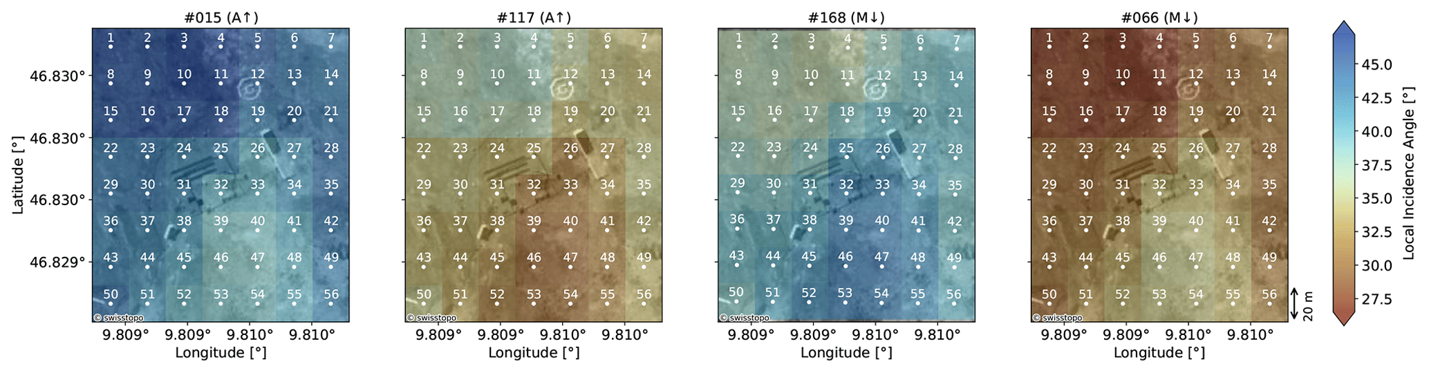
Figure 2 Overall range of local incidence angles across the study area for all the four relative orbits – morning/descending (M↓) and afternoon/ascending (A↑). Each S1 cell is identified by its centroid and a number.

The SAR images can be downloaded, free of charge, from the Copernicus data hub (, ). To account for the complex topography and to reduce the speckle noise of SAR acquisitions, a tailored preprocessing procedure was applied to all data. The processing procedure involves a combination of tools, some of which are available in SNAP (Sentinel Application Platform) version 6.0, while others are customized and developed in Python. The full workflow is described in Marin et al. (2020); however, in this study, the gamma-MAP filter was not applied. The final spatial resolution of the post-processed S1 images is 20×20 m.

The nominal radiometric uncertainty of S1 falls in the range of 3σ = 1.0 dB, as indicated in several ESA validation campaigns (Torres et al., 2012; Miranda et al., 2015; Schwerdt et al., 2017; Benninga et al., 2020). However, the overall radiometric accuracy is also affected by a number of preprocessing steps, including (but not limited to) the application of despeckle filters, terrain correction and radiometric normalization (particularly challenging in mountain regions with complex topography), and thermal noise removal (important in conditions of high absorption, such as wet snow). In such conditions, a detailed specification becomes extremely complex and falls beyond the scope of this paper. Nonetheless, since this study explores the multitemporal behaviour of ${\mathit{\sigma }}_{\mathrm{0}}^{\mathrm{VV}}$ over a target cell, it is relevant to mention speckle denoising. We used the filter proposed by Quegan and Yu (2001) – a powerful yet relatively simple one to denoise multitemporal stacks, with an 11×11 pixel window. Similarly to local spatial multi-looking, its implementation involves local averages of intensity values for each date. Intuitively, this could potentially blur strong targets and edges, ultimately leading to a loss of resolution and impacting the overall multitemporal result. However, in conditions of dry snow, the snow cover and the position of the scatterers are stable, snow temperatures are well below 0 °C and the soil should be mostly frozen, implying constrained variations in soil moisture. Under these conditions, the pixels we considered in our study exhibited an overall stable behaviour. The same stability was observed during dry periods in summer. In these two cases, the standard deviation was within 1.0 dB, which aligns with the nominal radiometric uncertainty of S1. During the melting period, the primary source of radiometric uncertainty originates from the formation of LWC within the snowpack. As a consequence, the radar return signal from the same target cell changes over time, resulting in reduced temporal coherence and larger deviations in multitemporal statistics. As will be shown in the course of this study, LWC potentially exhibits high heterogeneity across a single resolution cell. Under such conditions, the estimation of radiometric uncertainty becomes particularly challenging. Without a precise reference for LWC, rigorous uncertainty quantification is inherently difficult and lies beyond the scope of this work.

2.4 Campaign design

Measurements were carried out within freshly dug snow pits, starting at 08:00 (UTC+1) approximately. The start of the measurement procedure depended on the number of employees available on a specific day, on the amount of snow, on snow density and on the weather conditions – generally, between 1 and 2 h later. The measurement procedure was generally finished around 12:00 (UTC+1), and the snow pit was refilled; however, on isolated days, there were several hours of delay because of the above-mentioned reasons. In the first snow season, the snow temperature was generally measured first and the melting calorimetry last, with the remaining measurements being carried out in between with an order that also varied as a function of the above-mentioned factors. In the second snow season, we improved the campaign design with a more rigorous measurement order: temperature first, SSA and dielectric LWC either simultaneously or one after the other, density, SWE, and melting calorimetry coupled with a second simultaneous dielectric LWC profile taken at the same vertical location. This has specific importance for the LWC profiles. In the first season, the time lag between the dielectric and calorimetric LWC profiles was 2 or 3 h, at a horizontal distance of 50 cm to 1 m. In the second season, we measured a first dielectric LWC profile and an adjacent, simultaneous one using melting calorimetry. In Sect. 4.2, we will refer to the first setup as “co-located” and to the second one as “simultaneous”.

In both seasons, before starting the measurement procedure, the profile wall was made as smooth as possible. A near-infrared picture was taken for qualitative comparison. Outside of the snow pit, in an undisturbed area, the surface roughness panel pictures were taken. On days where the radiation (from the sun or diffuse) was particularly intense, shading was necessary for every surface measurement that might have been affected. The temperature profiles were always measured in the shaded corner area of the snow pit. Overall, each measurement series would need a total horizontal space of 1.5–1.8 m, and the single-variable profiles were measured at a reasonable horizontal distance from each other. In both seasons, snow profiles were carried out within the same designated area. The area was divided into corridors approximately 2 m wide. Throughout the season, measurements were carried out, moving continuously forward along the corridor until the slope was hit. The next snow profile would be dug onto the next corridor. A minimum distance of 30 cm was secured between 2 consecutive measurement days to avoid disturbances from the previous measurement set.

Data cleaning and homogenization procedures were performed before providing the measured snow properties as RT inputs. In particular, since sampling resolutions were different (see Sect. 2.1), all measured properties were linearly interpolated to a common vertical resolution of 1 cm. Positive LWC values recorded at temperatures below 0 °C were corrected to 0 %. 0.04 % and 0.4 % of the measured LWC values were above or equal to 15 % for the 2 years, respectively. For both dielectric instruments, these values are likely not accurate. Since these values likely represent areas of high snow wetness, they were not excluded from the analysis but their LWC value was set to 15 %, similarly to Techel and Pielmeier (2011). Additionally, instances of very low LWC measurements from thin layers just above the ground in dry snow conditions were discarded, as we could not rule out potential instrument disturbances from the ground in these cases. Given the accuracy range of the thermometer (see Sect. 2.1), temperature oscillations up to 0.2 °C below 0 °C were set to 0 °C from the first measured fully isothermal profile onwards. Since the snow properties were measured at a certain lateral distance from each other, the profiles of density and SSA were slightly shifted with a simple algorithm to maximize the correlation with the profile of LWC. Finally, we had to discard the last 3 snow pit measurements of 2023 because the measured RMSH value there was too high to ensure the conditions of validity of the interface model (see Sect. 3.2).

3 Methods and model

3.1 Selection of the Sentinel-1 reference cell

The selection of the reference S1 cell required some consideration. The WFJ field site is ideal for continuous measurements due to its proximity to structures and sensors; however, these features may interfere with radar waves, thus disrupting the backscatter from natural terrain. Most of the structures within the field site are metallic and may act as additional reflecting sources in addition to the snowpack.

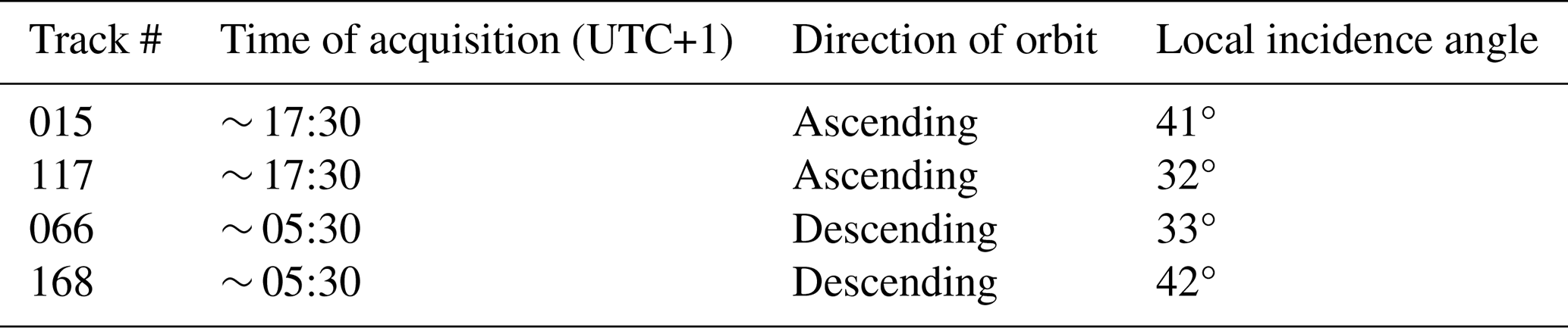
To select the reference cell, we extracted ${\mathit{\sigma }}_{\mathrm{0}}^{\mathrm{VV}}$ values for both years over a grid of 56 points covering the whole extension of the field site and the immediate surroundings (Fig. 3). For each cell and for each different year, we isolated the time frame, starting at the beginning of the meteorological winter (1 December) and ending when the first liquid water was measured in the snowpack. Over these time frames, for each year and for each cell, we computed the variability in ${\mathit{\sigma }}_{\mathrm{0}}^{\mathrm{VV}}$ acquired by the 4 different tracks (see Table 1). We assume that lower variabilities between different tracks over a dry snowpack may indicate a minimal interference with other non-natural elements in the field, as their backscatter would typically exhibit strong angular dependence (i.e. anisotropy).

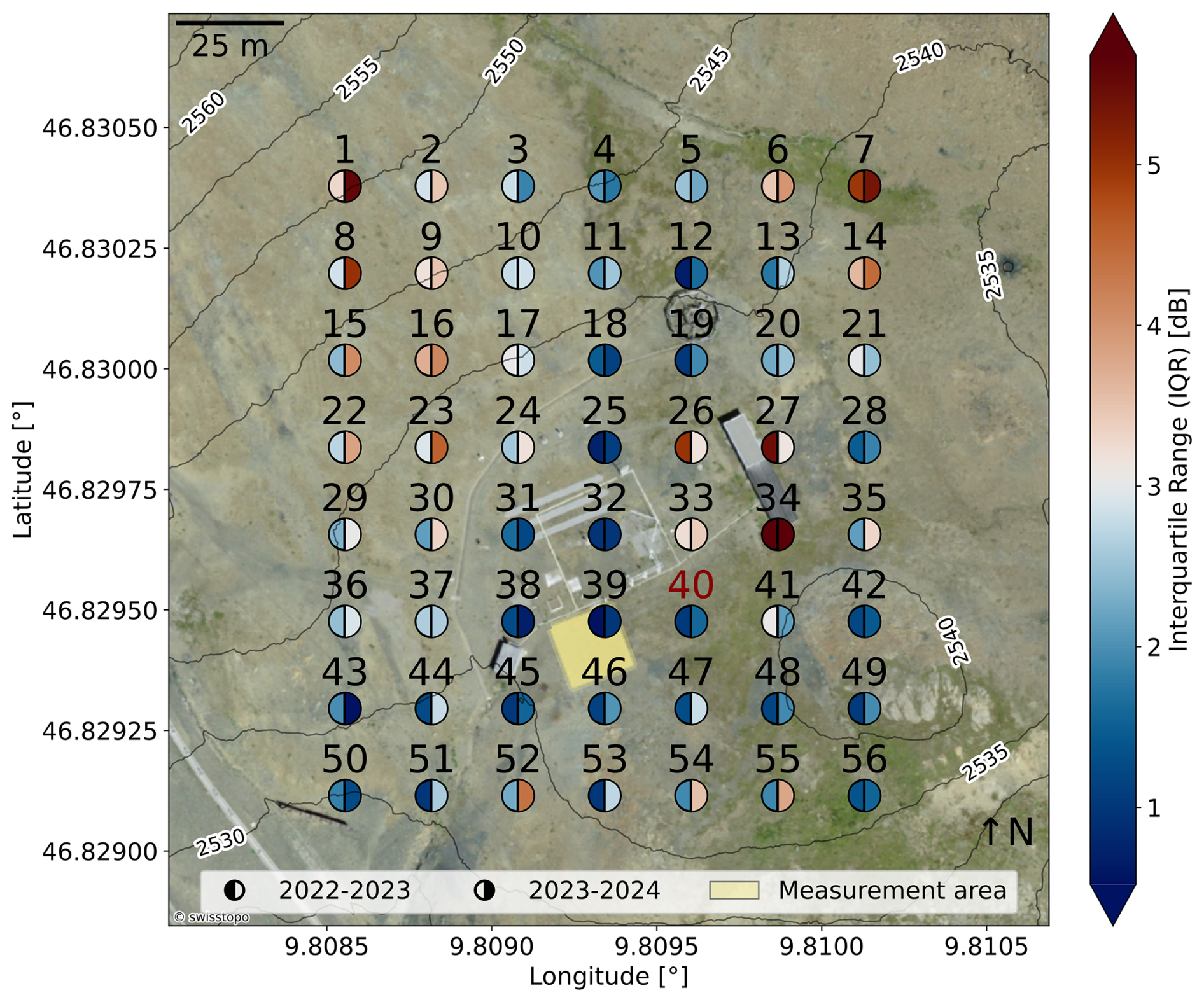
Figure 3 Aerial view of the WFJ measurement station. Each of the 56 points represents the centroid of each S1 cell. Each centroid is split in two, the left part indicating the interquartile range (IQR) of the winter ${\mathit{\sigma }}_{\mathrm{0}}^{\mathrm{VV}}$ signal for the snow season of 2022–2023 and the right part that for the snow season of 2023–2024. Contour lines indicate the surrounding slopes. The yellow rectangle indicates the fenced measurement area where snow profiles were carried out in both seasons. Cell 40, i.e. the selected S1 cell for this study, is highlighted in red.

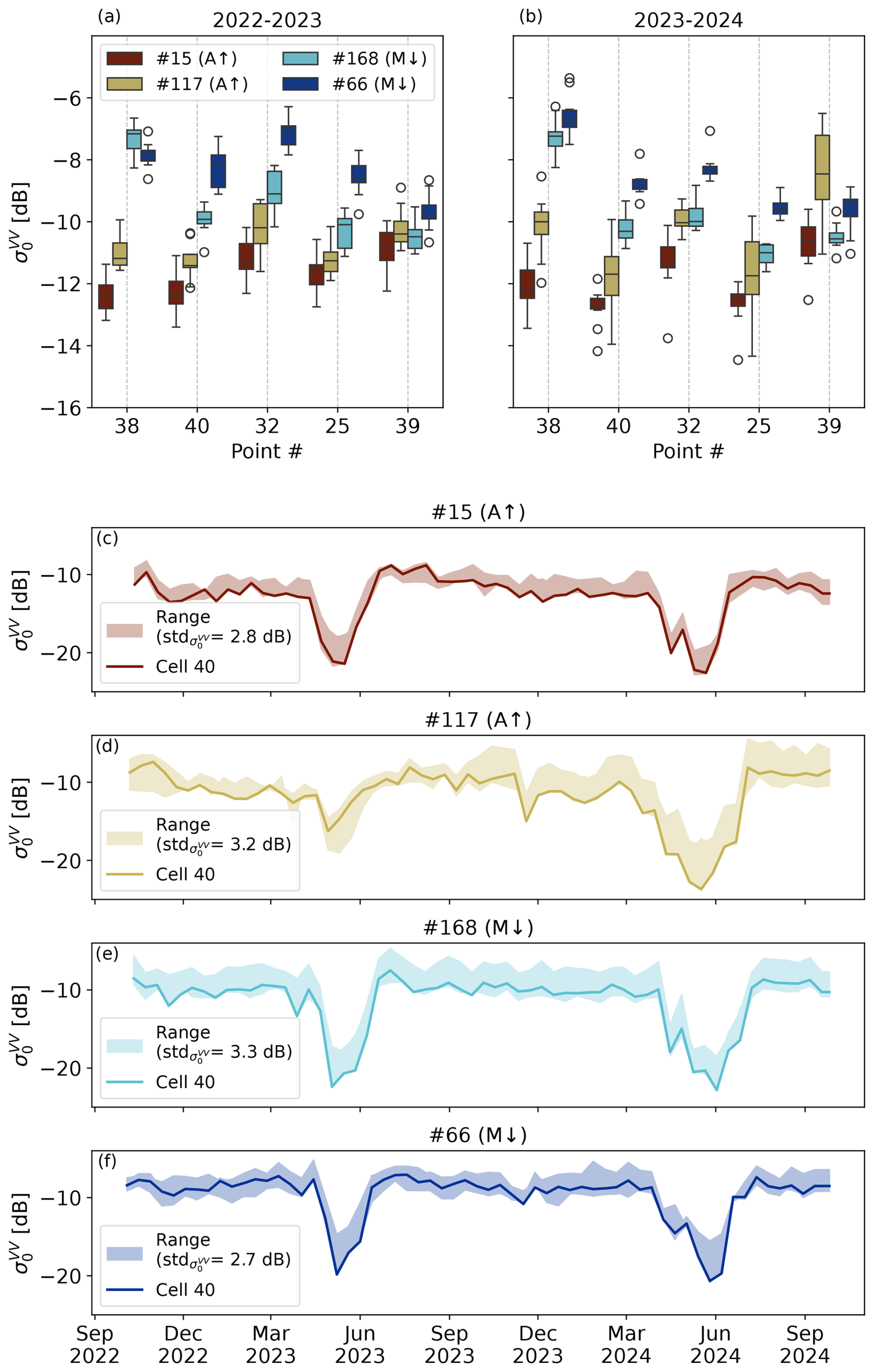
Figure 4 Variability in ${\mathit{\sigma }}_{\mathrm{0}}^{\mathrm{VV}}$ in dry snow conditions for all relative orbits overlooking cells 25, 32, 38, 39, and 40, i.e. the flat-terrain cells with likely similar snow properties to the measured ones (a–b). Multitemporal ${\mathit{\sigma }}_{\mathrm{0}}^{\mathrm{VV}}$ signal of the selected cell 40 compared to the ensemble standard deviation (std${}_{{\mathit{\sigma }}_{\mathrm{0}}^{\mathrm{VV}}}$) of the similar cells – morning/descending (M↓) and afternoon/ascending (A↑) (c–f).

Table 1 S1 tracks overlooking the selected cell 40, with times of acquisition, direction of orbit and local incidence angles.

The results of this analysis are shown in Fig. 3, where the variability is mapped over the field using the interquartile range (IQR). In general, the IQR does not vary significantly between the two snow seasons, suggesting that this kind of approach might be adequate to select a reference cell with the least possible artificial disturbance. Outliers – i.e. cells 15, 22, 23, 27, 52, 54, and 55 – are likely influenced by localized field conditions. These include double-bounce effects typically associated with human-made structures (e.g. cell 27), surfacing boulders (cells 52, 54, 55), or small variations in soil moisture, which could account for the observed year-to-year variability. The highest IQR values are clustered around the large hut (for double-bounce effects) and where the slopes start to become steeper (when the backscatter has its strongest dependence on the incidence angle). Interestingly, the IQR values for cell 25 and 32 are among the lowest for both snow seasons, suggesting that smaller metallic sensors might not represent a significant disturbance for radar waves.

Ideally, the target cell should coincide with the location of in situ measurements to ensure that the observed snow properties accurately represent those detected by the radar. Although the S1 footprint is large relative to the area disturbed by a single snow pit, excavating multiple consecutive snow profiles across a broader area can ultimately alter snow conditions across the entire cell – particularly under moist or wet snow conditions. This would introduce an uncontrolled degree of uncertainty. Therefore, the target cell should rather be selected from among the surrounding undisturbed cells with similar slopes and aspect. Figure 4a–b show the dry-snow ${\mathit{\sigma }}_{\mathrm{0}}^{\mathrm{VV}}$ variability for a set of cells with such features, i.e. cells 25, 38, 39, and 40. Among these, cell 40 shows a distinguished dependence on each incidence angle and orbit direction, along with relatively low variability in ${\mathit{\sigma }}_{\mathrm{0}}^{\mathrm{VV}}$ across tracks. An exception occurs for track #117 during 2023–2024, where the variability is relatively high with respect to the year before. This increased variability is also noticeable for cell 25 and 39. Given the lower variabilities recorded in the prior year, interference from non-natural elements can be ruled out. The most plausible explanation is a certain degree of heterogeneity in soil moisture across the field. Unfortunately, we are unable to verify this hypothesis, as soil moisture measurements were not included in our field campaign. Additionally, cell 40 lies in the immediate vicinity of the measurement site, and the snow surface remains undisturbed due to the operation of a LiDAR laser scanner continuously monitoring the snow surface. Figure 4c–f illustrate the multitemporal ${\mathit{\sigma }}_{\mathrm{0}}^{\mathrm{VV}}$ signal from cell 40 in comparison to that of the other candidate cells. The average standard deviation of the ${\mathit{\sigma }}_{\mathrm{0}}^{\mathrm{VV}}$ ensemble across these cells is approximately 3 dB for all tracks. Interestingly, the lowest standard deviation is consistently observed at the time of the backscatter drop caused by wet snow, with the exception of track #117 in 2024. Notably, during the melting season, the signal from cell 40 lies at the lower end of the backscatter range across all years and tracks – aside from track #117 in 2022–2023. Potentially, this behaviour is desirable for wet-snow detectability. For these reasons, the ${\mathit{\sigma }}_{\mathrm{0}}^{\mathrm{VV}}$ recorded over cell 40 is selected as the reference time series for this work.

The impact of the incidence angle was not a primary focus of this study, as it has already been extensively addressed in previous research (Mätzler, 1987; Shi and Dozier, 1992; Strozzi et al., 1997; Strozzi and Matzler, 1998) that strongly relied on tower-based instruments, allowing greater control than satellite-based radar systems. In our case, the most representative area for the measured snow properties is relatively small and flat, resulting in a limited range of local incidence angles available for analysis (see Fig. 2). Furthermore, the high spatial variability of LWC would require dedicated reference measurements for each incidence angle and cell, which was not feasible given the time and resources already involved in conducting the campaign at a single location.

3.2 Snow Microwave Radiative Transfer (SMRT) model: description and simulation setup

SMRT is a model that simulates the active–passive microwave response from layered snowpacks (Picard et al., 2018). The model is written and run in a Python environment and has a modular and flexible structure, allowing the user to set model runs by choosing from among a wide set of electromagnetic, microstructure and permittivity models. The reflectivity and transmissivity associated with roughness can also be described according to different models. The user has to specify a set of snowpack properties to parametrize the microstructure and the electromagnetic model. In particular, the roughness can be set either at the snow–air interface only or for each defined snow layer. Once these necessary parametrizations have been declared in the preliminary components of the model, SMRT uses the discrete ordinate and eigenvalue (DORT) method to solve the radiative transfer equation. The user can either customize a virtual sensor with specific frequency, incidence angle and polarization or directly choose from a list of already available sensors, among which S1 is included. The backscatter intensities can be obtained for all polarizations – this study focuses on the co-polarized vertical signal because cross-polarizations are currently only partially implemented within the current version of the module used for the parametrization of surface and interface scattering (Murfitt et al., 2024).

This study uses the symmetrized strong-contrast expansion (SymSCE) (Picard et al., 2022b) as the electromagnetic model with two different permittivity parametrizations. Measurements of density and SSA were used to compute the Porod length (ℓ_P) (Porod, 1951). The microwave grain size (ℓ_MW) is computed as the product of ℓ_P and the polydispersity k, a parameter describing the variability in the length scales with respect to the microstructure (Picard et al., 2022c). k was set to 0.75: this empirical value was estimated from μ-CT scans of a wide variety of alpine snow samples with convex grains, among which were rounded grains and melt forms (Picard et al., 2022c). For this study, snow microstructure was parametrized using the exponential model. For frequencies in the X- and Ku-bands (10–17 GHz), exponential autocorrelation functions have been shown to be too simplistic for representing snow microstructure. Their fast decay fails to capture long-range spatial correlations, and their inadequacy in modelling densely clustered media results in an underestimation of forward-scattering effects (Chang et al., 2016). However, Picard et al. (2022c) show how ℓ_MW can be computed analytically for various forms of autocorrelation functions, including the exponential. These analytical expressions of ℓ_MW allow for direct comparison between different representations of snow microstructure. Most importantly, when the same value of ℓ_MW is used as input, all microstructure models give the same scattering amplitude in the low-frequency limit. Therefore, according to these findings, the choice of the best representation of snow microstructure becomes a secondary problem with respect to measuring ℓ_MW in order to predict snow scattering in the C-band.

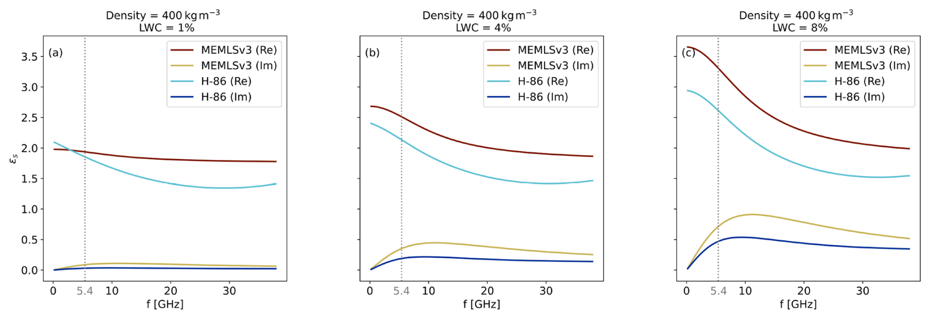
Figure 5 Real and imaginary parts of the effective permittivity (ϵ_s) of wet snow as a function of frequency (f) for a nominal density value of 400 kg m⁻³ and varying LWC of 1 % (a), 4 % (b) and 8 % (c) according to the MEMLSv3 and H-86 permittivity models. Dotted grey lines underline differences between the formulations at the nominal frequency of S1, i.e. 5.405 GHz.

The permittivity of a material is a complex number composed of a real part (i.e. the dielectric constant) and an imaginary part. The contribution of the real part is related to the material's ability to store electrical energy, whereas the contribution of the imaginary part is associated with dielectric losses. Snow is a three-component mixture of ice, air and water – therefore, the effective permittivity of snow (ϵ_s) depends on the relative proportions of these elements. The presence of liquid water significantly alters both the real and the imaginary parts of ϵ_s, affecting how microwaves interact with the snowpack. Henceforth, accurate estimates of ϵ_s are crucial for interpreting the microwave response of wet snow. Despite extensive research, particularly in the 1980s, a universally accepted model for snow permittivity has not yet been established (Picard et al., 2022a). For this study, we selected two formulations: (i) the Microwave Emission Model for Layered Snowpacks (Wiesmann and Mätzler, 1999) in its third version (MEMLSv3 hereafter), which is based on the Maxwell Garnett mixing theory of dry snow and prolate water inclusions, and (ii) the Debye-like model modified by Hallikainen et al. (1986) (H-86 hereafter), which uses a mixing formula based on volume fractions and refractive indices, calibrated against field data. These models were selected because they were validated against real-world C-band data. Specifically, in Hallikainen et al. (1986) and earlier works, the authors present what is, to our knowledge, the only available dataset of wet-snow permittivity measurements at 6 GHz for varying LWC values, measured using freezing calorimetry. Interestingly, MEMLSv3 fails to accurately reproduce this dataset. However, Kendra et al. (1998) observed that the dielectric constant provided by H-86 appears to be too low, an observation that is supported by data from Achammer and Denoth (1994), collected in the range between 8 and 12 GHz. However, these data appear to favour H-86 over MEMLSv3 when considering the imaginary part of ϵ_s. While H-86 has been criticized, some aspects appear to have been overlooked (e.g. the recent corrigendum in Picard et al., 2022a). Figure 5 shows the real and imaginary parts of the ϵ_s as a function of the frequency for a nominal density value and varying values of LWC according to both MEMLSv3 and H-86 permittivity formulations. For higher values of LWC (see Fig. 5b, c), the ϵ_s values obtained from both formulations display a frequency dependence and curve shape closely resembling that of pure water. In both cases, the real part of ϵ_s decreases with frequency, whereas the imaginary part increases of up to the relaxation frequency and decreases thereafter. However, in the C-band, the two formulations diverge significantly, especially in their prediction of the imaginary part, which governs absorption losses. This difference becomes more pronounced for increasing values of LWC. For instance, at LWC = 4 %, MEMLSv3 predicts an imaginary part of ϵ_s approximately twice that of the H-86 at the nominal frequency of S1 (see Fig. 5b). Since we cannot definitively determine the fitness of one model over the other, both formulations will be used in SMRT for this study. Given the different behaviour of the two formulations, we expect a lower and upper bound for S1 backscatter simulations. It is clear that further research is needed to accurately characterize wet-snow permittivity, but this is out of the scope of this paper.

RT modelling of snow comes with the additional difficulty of quantifying the dense medium effects, i.e. the electromagnetic interactions occurring between snow grains that are closely packed together. At C-band frequencies, these effects become significant as the scattering regime changes due to the presence of liquid water – through changes both in snow grain interactions and in bulk dielectric properties. In H-86, dense medium effects are not accounted for. In MEMLSv3, these effects are accounted for through a semi-empirical parametrization involving, among other parameters, correlation length, density-dependent corrections and – as mentioned above – mixing formulas. Correlation lengths are used to represent the effective grain size and spatial correlation of the ice matrix and to capture the degree of interaction between dense grains. Despite the range of correlation lengths being limited in MEMLSv3, the ones that are represented are derived from structures observed at Weissfluhjoch during two snow seasons (Wiesmann and Mätzler, 1999). Therefore, they are likely suitable to describe the dense medium effects on the snowpack structures observed and measured in this study. Snow density is used as a proxy to determine how closely grains are packed; and as density increases, scattering is reduced and absorption increases. Such corrections are embedded into the extinction term, i.e. the sum of scattering and absorption coefficients.

The chosen interface model (between snow and air and between snow layers) is the integral equation model (IEM) (Brogioni et al., 2010), since it is one of the most used models to describe the roughness. However, any other model could be used, provided the roughness characteristics are within the validity range. The IEM is valid under the conditions $w\cdot \mathrm{RMSH}<\mathrm{2}$ and $w^{\mathrm{2}}\cdot \mathrm{RMSH}\cdot \mathrm{CL}<\sqrt{{\mathit{\epsilon }}_i}$, where w is the wavenumber (which depends on the medium) and ε_i is the ratio between the media permittivities at the interface (Fung et al., 1992).

Using the functions available in SMRT, we modelled the substrate as a reflecting surface with a given value of backscatter. In dry snow conditions, on days when manual measurements and satellite overlooks coincided, we assigned the S1 recorded backscatter value to the substrate, assuming that dry snow is transparent to radar waves at C-band and that therefore the soil is the only contribution to the total backscatter. In wet snow conditions (or in dry snow conditions when there was no concomitance between measurements and satellite overlooks), we assigned a fixed value of backscatter to the substrate, which we computed as the average value in dry snow conditions of each individual track (incidence angle). Notably, SMRT offers the possibility of computing the backscatter from the soil; however, it requires a series of detailed information that is spatially heterogeneous and would have been nearly impossible to retrieve continuously over the course of our campaign. These properties include the soil moisture, the relative sand content, the relative clay content, the soil content in dry matter, and other geometrical parameters such as the roughness and the correlation length.

Under these configurations, the model takes as inputs the following snowpack properties: temperature, density, volumetric liquid water, SSA and surface roughness. For the snow–air interface, we used the measured values of RMSH and correlation length. For layer interfaces, we set RMSH_layers=1 mm and CL_layers=30 mm (i.e. the average winter value from our field measurements). When measurements and S1 overpasses coincided, the simulation was performed using the incidence angle of S1. On days without simultaneous overpasses, the simulation was performed using the incidence angle from the closest previous or subsequent S1 pass. All modelling choices described above have been designed and motivated to be optimal to describe wet snow starting from measured properties. However, it is important to remark that the choice of such parametrizations remains highly arbitrary, as further research is still needed to validate permittivity, roughness and microstructure models specifically for wet snow in the C-band.

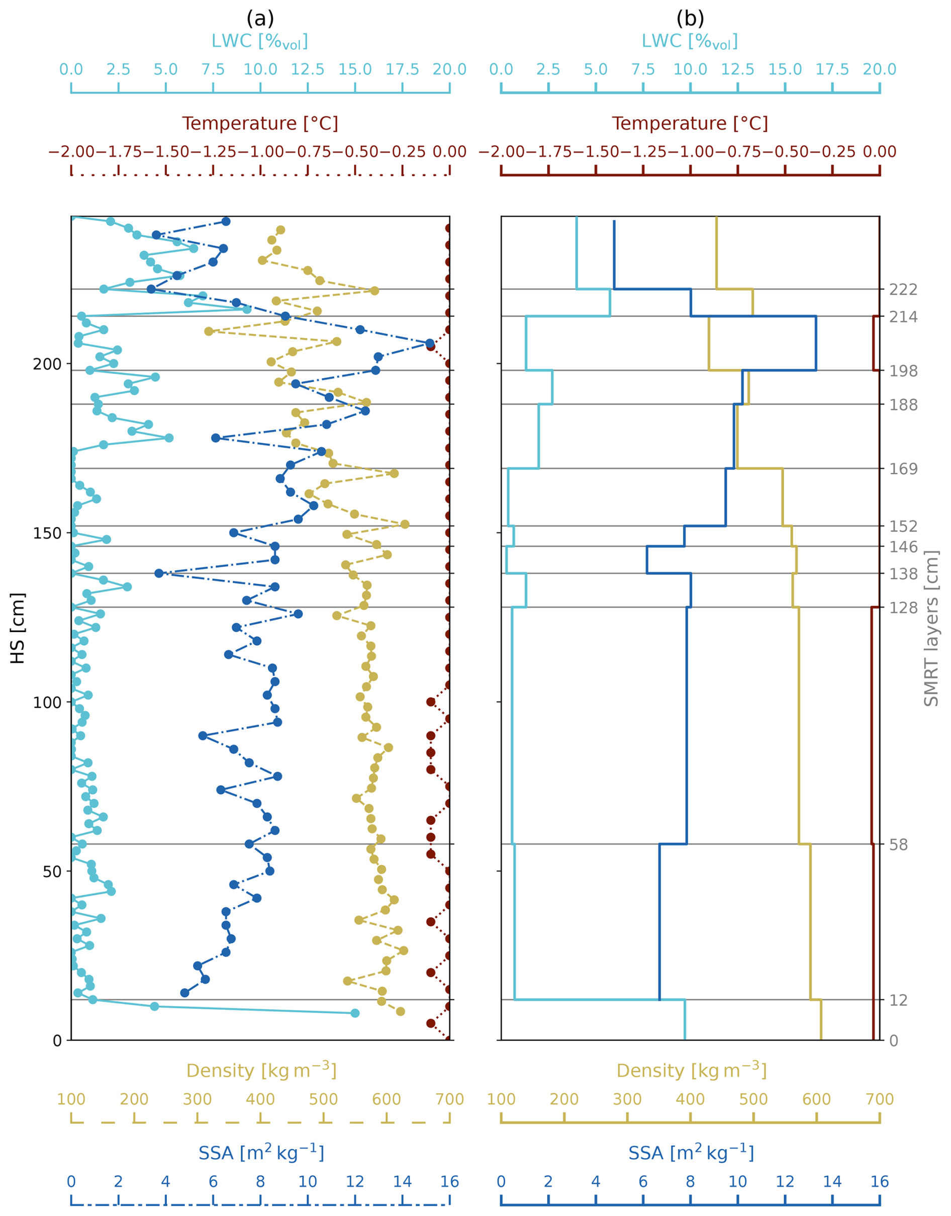
Figure 6 (a) Vertical profiles of snowpack properties measured in the field on 14 May 2024: temperature (dark red), density (dark yellow), liquid water content (LWC; light blue) and specific surface area (SSA; dark blue). The vertical spacing of the points connected by the lines reflects the measurement resolution for each profile: 5 cm for temperature, 3 cm for density, 2 cm for LWC and 4 cm for SSA. (b) Representation of the same profiles averaged according to the physically consistent snow layers (indicated by grey horizontal lines). The layered profiles as in (b) form the input snowpack for the SMRT model, combined with surface roughness parameters measured on the same day (RMSH = 2.7 mm; CL = 48.5 mm).

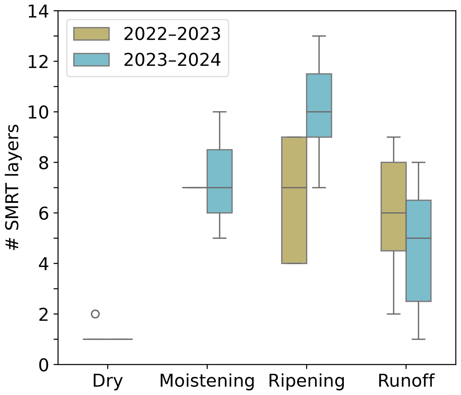
Figure 7 Variability in the number of modelling layers in SMRT used for each simulation day as a function of the melting phase and the campaign year.

Another practical challenge was to design a way to replicate the often complex snowpack layering observed in the field within a radiative transfer model which is not specifically made to deal with a high number of layers thinner than the wavelength (Sandells et al., 2022). As a matter of fact, this increases the number of dielectrical discontinuities (Leduc-Leballeur et al., 2015), generating (artificially) higher scattering. Resampling high-resolution field measurements to the wavelength or its multiples is an option; however, this does not necessarily reflect the physical snowpack structure. As an example, in the moistening phase, liquid water appears in thin layers in the upper part of the snowpack. These layers can have thicknesses of a smaller size than the C-band wavelength – the effect of such layers on the total backscatter is unclear and represents a potential source of errors when using layering defined by the resolution of the field measurements. As the wetting front progresses through the snowpack during the ripening phase, liquid water becomes more homogeneous over layers with thickness comparable to the C-band wavelength. During this stage, using high-resolution discretizations (e.g. on the order of the C-band wavelength) may seem appropriate to closely replicate the liquid water layering observed in the field. However, averaging over such scales can merge distinct wet and dry layers, blur important contrasts, and potentially lead to biased backscatter estimates. On the other hand, intuitively, lower-resolution discretizations (e.g. multiples of the C-band wavelength) dissipate the scattering effect of thinner (≃ 6 cm) wet layers. To reduce the aforementioned sources of uncertainty, we chose to model the snowpack structure by stacking layers with a minimum thickness corresponding to the C-band wavelength, ensuring each layer had consistent average physical properties. These physically similar layers were identified automatically by means of a simple algorithm and then refined manually, with particular emphasis placed on LWC over the other variables. An example is provided in Fig. 6, where snow properties are shown at the field-measured vertical resolution in (a) and averaged into physically consistent layers for SMRT input in (b). Figure 7 shows that the number of layers used for each SMRT simulation varied between 1 and 14, with a marked dependence on the stage of the melting process and on the campaign year. In dry snow conditions, the densely measured snow properties are practically always averaged into one single layer, given the absence of liquid water. As the snowpack starts moistening, the number of distinct layers increases, as a function of the first formation of liquid water within the snowpack. The highest number of layers required in SMRT to model the snowpack is used during the ripening phase, as the LWC layering is at its most heterogeneous state during this phase, as a consequence of the progression of the wetting front. Later in the runoff stage, with the snowpack being fully saturated, the number of SMRT layers used decreases again, as a consequence of a more homogeneously moist snowpack. On the other hand, Fig. 7 shows that during the ripening phase, the first campaign year has been modelled using ∼ 30 % fewer layers than the second, on average. The presence of ice lenses helped to homogenize the distribution of liquid water within the snowpack, resulting in more uniformly wet layers near the surface and consistently drier sections towards the bottom. Without ice lenses, in 2024, the progression of liquid water into the snowpack was more heterogeneous, therefore requiring more layers in the model to remain as true as possible to the conditions observed in the field. Despite the efforts to find a reasonable compromise between all the above-mentioned constraints, the optimal way to model a radar-equivalent snowpack from field measurements and/or detailed multilayer physical model outputs remains an open question in the field of radiative transfer modelling of snow, only recently addressed by Meloche et al. (2025), albeit for dry snow only.

4 Results

4.1 Identification and redefinition of melting phases from multitemporal Sentinel-1 backscatter and field measurements

Figures 8–9 show the evolution of the multitemporal S1 SAR backscatter together with the time series of measured properties: snow temperature, LWC, air temperature, total water content (TWC), runoff, snow water equivalent (SWE) and surface roughness indices (RMSH and CL). The melting phases identified with the method proposed by Marin et al. (2020) are reported for each time series for later validation. We will refer to the snow seasons of 2022–2023 and 2023–2024 as the 2023 and 2024 seasons, respectively.

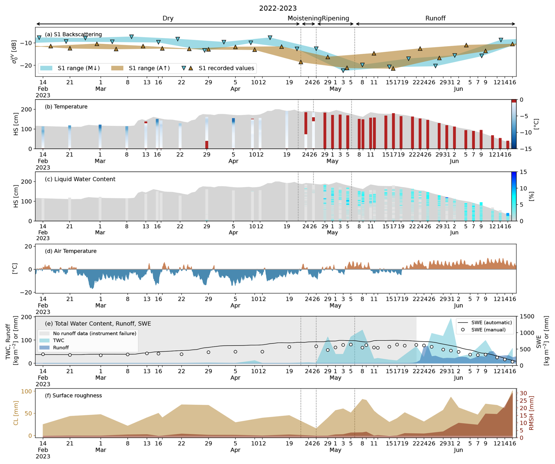
Figure 8 Data overview for the snow season of 2022–2023. (a) S1 backscatter time series: exact values of ${\mathit{\sigma }}_{\mathrm{0}}^{\mathrm{VV}}$ acquisitions (triangles); range obtained by connecting the consecutive S1 passages by direction of orbits, i.e. by connecting all the morning/descending (M↓) and the afternoon/ascending (A↑) acquisitions (shaded areas). Each panel is subdivided into the melting phases identified with the method of Marin et al. (2020). (b) Manually measured profiles of snow temperature. (c) Manually measured profiles of snow liquid water content (LWC). (d) Air temperature at hourly resolution, measured by the automatic sensor at WFJ. (e) Measured total water content (TWC) (light blue); runoff time series automatically recorded by the lysimeter at WFJ (dark blue); lack of runoff data due to the instrument failure (grey area); snow water equivalent (SWE) both automatically recorded by the snow scale (black line) and manually measured (white circles). (f) Time series of measured surface roughness parameters – RMSH and CL.

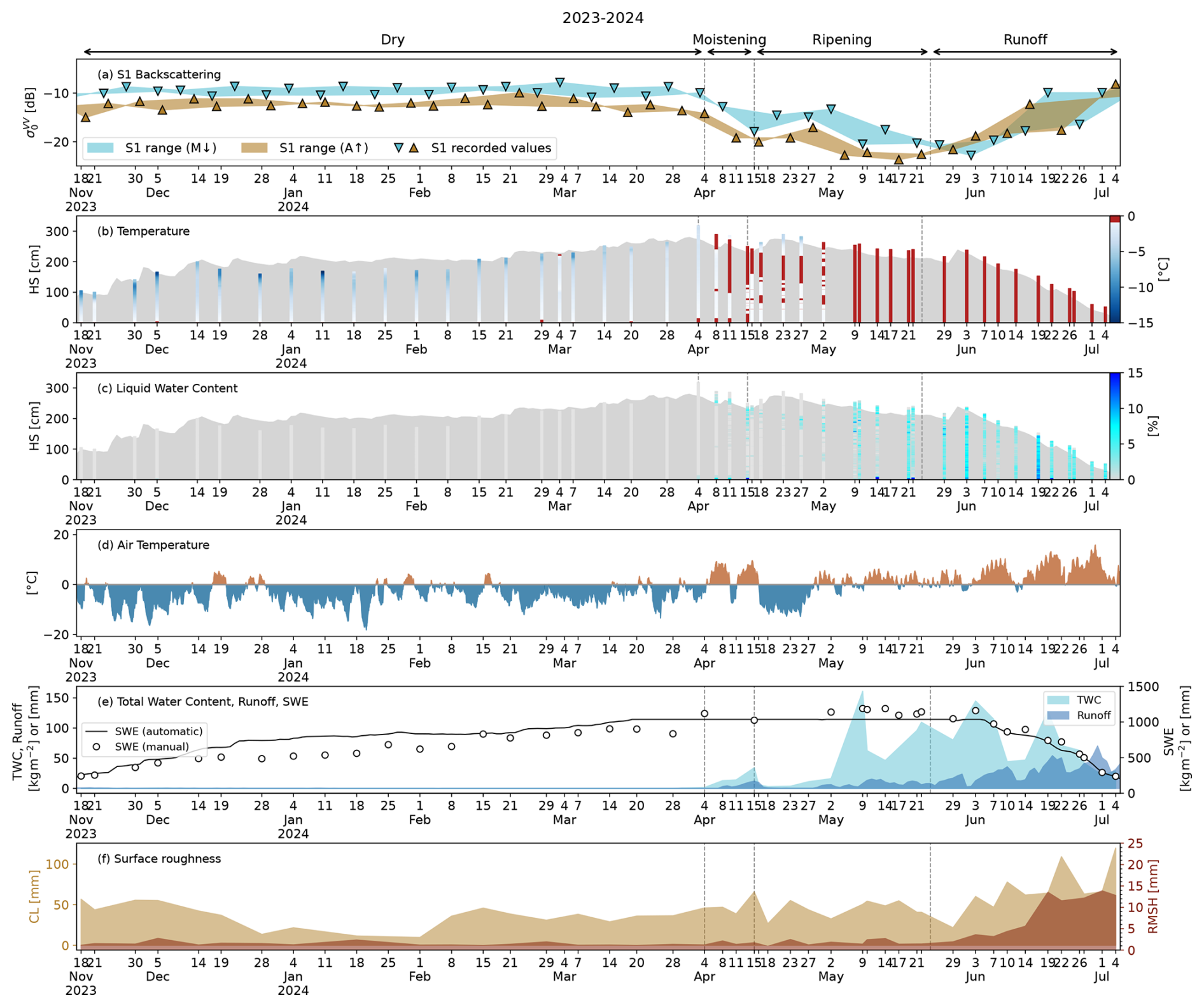
Figure 9 Data overview for the snow season of 2023–2024. (a) S1 backscatter time series: exact values of ${\mathit{\sigma }}_{\mathrm{0}}^{\mathrm{VV}}$ acquisitions (triangles); range obtained by connecting the consecutive S1 passages by direction of orbits, i.e. by connecting all the morning/descending and the afternoon/ascending acquisitions (shaded areas). Each panel is subdivided into the melting phases identified with the method of Marin et al. (2020). (b) Manually measured profiles of snow temperature. (c) Manually measured profiles of snow liquid water content (LWC). (d) Air temperature at hourly resolution, measured by the automatic sensor at WFJ. (e) Measured total water content (TWC) (light blue); runoff time series automatically recorded by the lysimeter at WFJ (dark blue); snow water equivalent (SWE) both automatically recorded by the snow scale (black line) and manually measured (white circles). (e) Time series of measured surface roughness parameters – RMSH and CL.

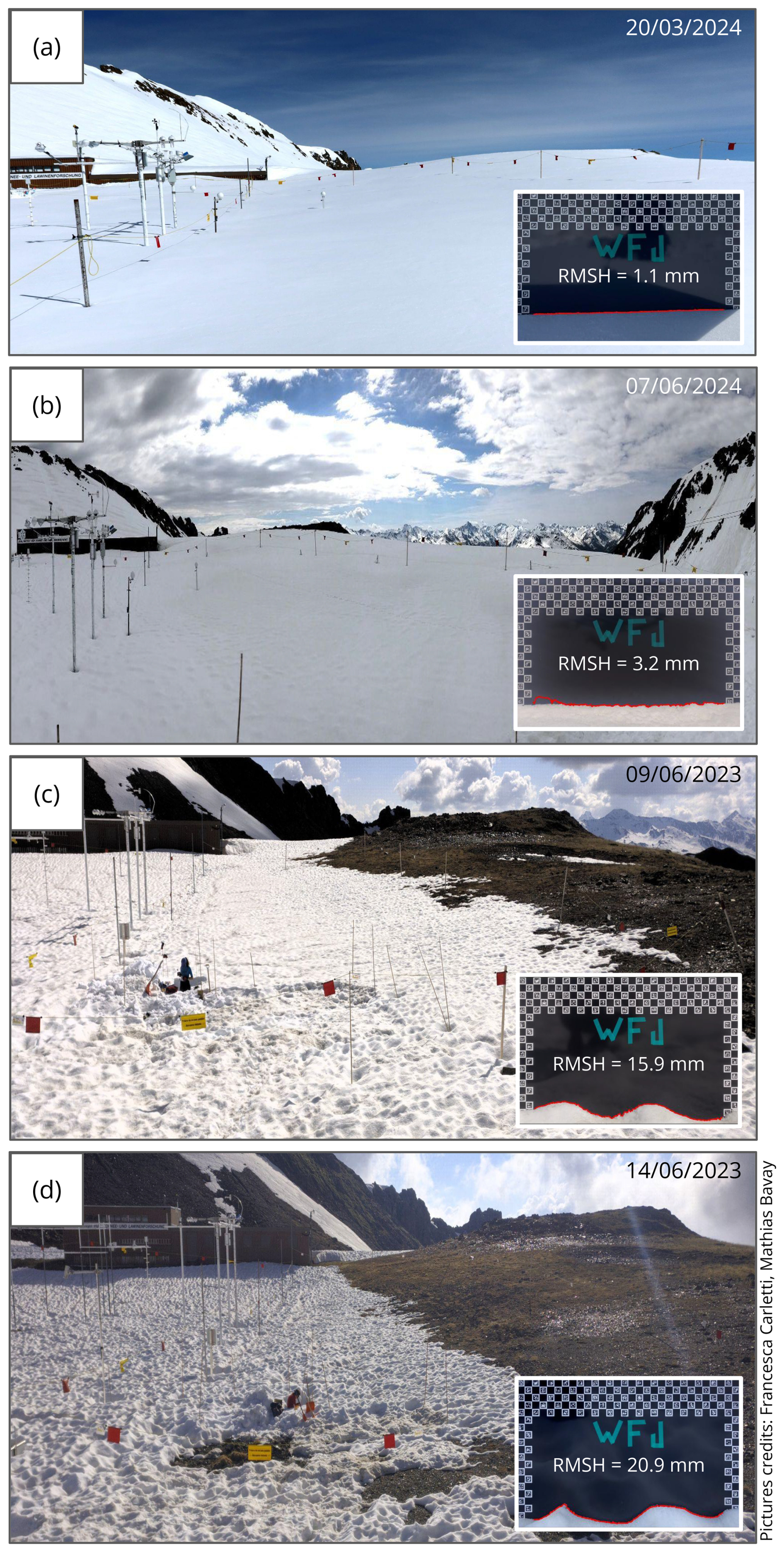
Figure 10 The panels illustrate some representative surface roughness conditions as qualitatively observed on the field (panoramic pictures) together with one of the panel measurements performed on the same day (bottom right of each panel, where the mean roughness RMSH measured on that day is also reported). (a) Smooth surface typical of dry snowpack conditions. (b) Early-stage development of surface roughness deriving from melt–refreeze cycles. (c) Fully formed suncups over a homogeneous snow cover, at least at the considered S1 cell. (d) Fully formed suncups over a patchy snow cover.

Our roughness measurements show clear differences for different snow surfaces (Fig. 10). Smooth surfaces typical of new/dry snow have RMSH values around 1 mm (Fig. 10a). Thereafter, roughness increases with increasing surface degradation due to melt–refreeze cycles and sublimation (Fig. 10b). The values of RMSH measured in these conditions, which are the most persistent throughout the melt season, lie within approximately 3 and 10 mm. Fully formed suncups are associated with values of RMSH around 10–15 mm (Fig. 10c). Deep suncups appear like craters on the snow surface (Fig. 10d), some reaching widths of 20 cm and depths of 10 cm. In these conditions, we measured values of roughness RMSH equal to or higher than 20 mm.

In 2023, the first liquid water was measured on 10 April (Fig. 8b). On this date, our data show that the temperature of the top ∼ 5 cm of the snowpack was 0 °C (Fig. 8b). The air temperature reached 0 °C as well on this day (Fig. 8d). The snowpack reached the full isothermal state 20 calendar days later. Ice layers formed throughout the season, likely as a consequence of repeated melt–refreeze cycles and the succession of several warm and cold spells (Fig. 8d). Ice layers were observed regularly during the measurement campaign; their presence is highlighted by locally higher values of LWC due to ponding at approximately 100 cm from the ground. The presence of ice layers probably withheld the meltwater in the upper section of the snowpack, partially hindering the progression of the wetting front. LWC profiles in Fig. 8c highlight ponding above ice layers consistently until 15 May. The ponding is no longer detected over the next consecutive 5 snow profiles and becomes visible again from 26 May until early June, when the ice layers likely disintegrated, allowing the meltwater to percolate to the bottom of the snowpack. The fact that the ponding above ice layers is not detected on a series of consecutive snow profiles is probably linked to the partial refreeze of the snowpack highlighted by the drop in air temperature detected within this time span (Fig. 8d). However, ice layers could also be laterally non-homogeneous. Figure 8f shows that the roughness associated with wet snow starts developing shortly after the snowpack starts moistening, with RMSH increasing until 9 May. Thereafter, the cold spell brought new snowfalls, which smoothened the snow surface significantly, and roughness indices reverted to typically winter values for approximately 10 calendar days. Fully formed suncups were observed on the field from 31 May onwards. As explained in Sect. 2.2, the lysimeter time series for 2023 (Fig. 8e) is not useful for detecting the runoff start. However, both manual and automatic measurements indicate the first slight snow depth (HS) and SWE decrease around 8 May, following a warm spell that lasted several days. This occurred in the presence of a fully isothermal snowpack, suggesting that runoff may have started to be released around this time.

In 2024, the first liquid water on the surface was measured on 8 April during a warm spell (Fig. 9b–d). From this date on, the wetting front moved somewhat into the snow before being interrupted by a cold spell, which caused a partial surface refreeze. The snowpack reached the full isothermal state on 9 May. Over the course of this season, ice layers were not observed in the field, the progression of the wetting front was not hindered and the snowpack reached full saturation earlier with respect to the previous year. The runoff time series confirms that the snowpack released the first meltwater around 8 April. It should be noted, however, that this early release represents not the runoff onset but rather the preferential flow of initial meltwater reaching the bottom of the snowpack. On this date, the (pointwise) measurements show a largely isothermal snowpack. Likely, the snowpack was isothermal over the entire cell (Fig. 9b, c, e). Additionally, significant amounts of LWC were measured at the ground interface after 8 April, and the manual measurements show a SWE decrease of ≃ 100 mm between 4 and 15 April. Runoff began steadily in early May, when a significant amount of water was measured at the bottom of the fully isothermal snowpack, along with decreases in HS and SWE. These observations can validate the hypothesis made for the previous season in the absence of runoff data due to instrument failure. Our measurements in Fig. 9f show that surface roughness increased relatively late (3 June) with respect to the previous season, with fully formed suncups being visible on the field from 19 June onwards.

Coupling the detailed, high-temporal-resolution information about the state of the snowpack with the multitemporal SAR ${\mathit{\sigma }}_{\mathrm{0}}^{\mathrm{VV}}$ recorded by S1 on morning and afternoon overpasses (Figs. 8–9a) enables the validation of the methodology proposed by Marin et al. (2020) to identify the melting phases. According to the authors, a drop of at least 2 dB with respect to the winter mean in the afternoon/ascending ${\mathit{\sigma }}_{\mathrm{0}}^{\mathrm{VV}}$ identifies the start of the moistening phase, the ripening phase starts when the morning/descending ${\mathit{\sigma }}_{\mathrm{0}}^{\mathrm{VV}}$ signal shows the same drop of at least 2 dB, and the runoff starts when both morning/descending and afternoon/ascending ${\mathit{\sigma }}_{\mathrm{0}}^{\mathrm{VV}}$ time series reach their local minima before the monotonic increase (the authors propose an average date between the two local minima when both the S1 satellites were available). For the two seasons, we computed the average winter backscatter ($\stackrel{\mathrm{‾}}{{\mathit{\sigma }}_{\mathrm{0},\mathrm{dry}}^{\mathrm{VV}}}$) by averaging all values recorded by each individual track over the course of the meteorological winter, i.e. from 1 December to 28 February. The resulting values are the benchmark needed to identify the melting phases. The results are listed in Table 2. As noted by Marin et al. (2020), the dependence of ${\mathit{\sigma }}_{\mathrm{0}}^{\mathrm{VV}}$ on incident angles remains as a residual effect.

(Marin et al., 2020)

Table 2 Overview of the identification of the melting phases based on the multitemporal S1 SAR backscatter as proposed by Marin et al. (2020). For each season, the table shows the relevant values of ${\mathit{\sigma }}_{\mathrm{0}}^{\mathrm{VV}}$ and the occurrence dates for each afternoon/ascending (A↑) and morning/descending (M↓) look (and corresponding incidence angle). The selected values for the start of the moistening, ripening and runoff phases are highlighted in bold. For the runoff start, the selected date according to the method of Marin et al. (2020) is compared against the data recorded by the lysimeter, when available.

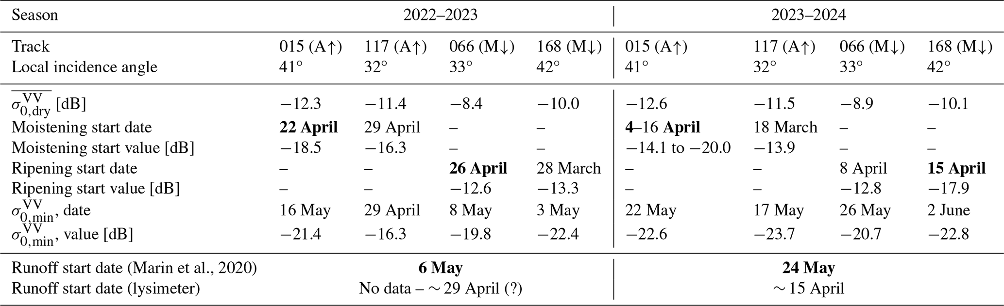
Because, for the selected cell, two morning/descending and afternoon/ascending looks are available, there are two possible dates for the start of the moistening and ripening phase, respectively. In 2023, these dates are 22 and 29 April for the moistening phase and 28 March and 26 April for the ripening phase. For the start of the moistening phase, we selected the earliest, i.e. 22 April. For the start of the ripening phase, the two identified dates are almost 1 month apart; however, the ${\mathit{\sigma }}_{\mathrm{0}}^{\mathrm{VV}}$ decrease recorded on 28 March by track #168 is caused by a warm spell, as the following value recorded by the same track aligns approximately with the winter mean again. Therefore, we selected 26 April as the start of the ripening phase. In 2024, for the moistening phase, the ${\mathit{\sigma }}_{\mathrm{0}}^{\mathrm{VV}}$ value recorded on 4 April by track #015 is only 1.5 dB lower than $\stackrel{\mathrm{‾}}{{\mathit{\sigma }}_{\mathrm{0},\mathrm{dry}}^{\mathrm{VV}}}$; however, the next passage of the same track on 16 April recorded a drop of 7.4 dB already. Therefore, the moistening start has been placed on 4 April. On this date, track #117 recorded a drop of 7 dB with respect to $\stackrel{\mathrm{‾}}{{\mathit{\sigma }}_{\mathrm{0},\mathrm{dry}}^{\mathrm{VV}}}$. For the ripening start, we chose 15 April.

These considerations show that the method of Marin et al. (2020) is limited by the halved S1 revisit frequency. This becomes even more clear for the selection of the runoff start date, as the wider separation between local minima of ${\mathit{\sigma }}_{\mathrm{0}}^{\mathrm{VV}}$ considering all 4 looks is 17 calendar days for 2023 and 16 calendar days for 2024. Using the date in between to determine the runoff start, as done by Marin et al. (2020), gives potentially unreliable results in these conditions. This low temporal resolution makes it difficult to pinpoint precise onset dates, especially when minima are separated by such long periods. Despite the ambiguities, in both seasons, the identified moistening phase coincides exactly with the first snowpack warming and the consequent formation of liquid water. The identified ripening phase is also mostly consistent with the theory, as field measurements show that the snowpack transitions to the fully isothermal state with the wetting front progressing to the bottom, although this process is partially hindered in 2023 by ice layers. In 2024, a sudden cold spell at the beginning of the ripening phase caused the refreezing of the superficial meltwater (Fig. 9b–d). This generated a sharp increase in both morning and afternoon ${\mathit{\sigma }}_{\mathrm{0}}^{\mathrm{VV}}$ (Fig. 9a). In 2024, the first instance of measuring a fully isothermal snowpack coincided precisely with the first afternoon local minimum of ${\mathit{\sigma }}_{\mathrm{0}}^{\mathrm{VV}}$. The same cannot be verified for 2023, which instead shows a counterintuitive case where the local minimum of morning ${\mathit{\sigma }}_{\mathrm{0}}^{\mathrm{VV}}$ anticipates the local minimum of afternoon ${\mathit{\sigma }}_{\mathrm{0}}^{\mathrm{VV}}$ (Fig. 8a). Nonetheless, by the time the morning ${\mathit{\sigma }}_{\mathrm{0}}^{\mathrm{VV}}$ reached its local minimum in 2023, the snowpack had already been fully isothermal for at least 5 calendar days (Fig. 8a–b). This suggests that the snowpack is likely to be fully isothermal when the afternoon ${\mathit{\sigma }}_{\mathrm{0}}^{\mathrm{VV}}$ reaches its local minimum. The runoff time series in 2024 shows that the snowpack had started to release meltwater as soon as it was in the late moistening phase (Fig. 9e), in correspondence to the first local minimum of the afternoon ${\mathit{\sigma }}_{\mathrm{0}}^{\mathrm{VV}}$ time series on 16 April (Fig. 9a). However, as clarified above, this initial release does not mark the onset of runoff, which begins consistently in early May.

Marin et al. (2020) proposed three possible explanations for the monotonic backscatter increase following the local minima: (i) the increase in surface roughness, (ii) the decrease in TWC, and (iii) the snow cover gradually becoming patchy. Our data show that over a high-altitude alpine snowpack like the study plot at WFJ, roughness develops on the snow surface well before the snow cover begins to disappear in patches. Therefore, at least for similar altitudes, the gradual disappearance of the snow cover can be ruled out as a cause of the increasing backscatter in the late melting stage. For both seasons, our data indicate that the strongest correlation with the monotonic increase in ${\mathit{\sigma }}_{\mathrm{0}}^{\mathrm{VV}}$ after the local minimum is observed with the gradual increase in surface roughness (Figs. 8–9f). Conversely, there seem to be no remarkable correlations between the increase in ${\mathit{\sigma }}_{\mathrm{0}}^{\mathrm{VV}}$ and the TWC and/or runoff trends. In fact, Figs. 8–9e show that the decrease in TWC as a consequence of snow ablation is not monotonous. On the other hand, both automatic and manual measurements show that by the time SWE started decreasing sharply and monotonically (around 26 May 2023 and 6 June 2024), the S1 ${\mathit{\sigma }}_{\mathrm{0}}^{\mathrm{VV}}$ had already increased again by ≃ 6 dB.

4.2 Instrumental uncertainty and variability in field measurements of liquid water content

Figure 5 shows that liquid water has a strong impact on the real and imaginary parts of ϵ_s at C-band frequencies. For S1 ${\mathit{\sigma }}_{\mathrm{0}}^{\mathrm{VV}}$ retrievals from ground measurements, this poses three major challenges. In the first place, manual measurements concern a very small area/volume, whereas satellite acquisitions cover a pixel size of 20×20 m. Secondly, the distribution of liquid water within the snowpack can be highly heterogeneous because of a variety of features and processes, namely capillary barriers, preferential flows and ice layers. Finally, what is the most accurate methodology for measuring LWC in both lab and field environments remains a debated question in snow science (Barella et al., 2024), and although the methods used in this paper were designed to achieve a good level of robustness, they are nevertheless subject to error. Therefore, all these uncertainty sources need to be taken into account when comparing satellite ${\mathit{\sigma }}_{\mathrm{0}}^{\mathrm{VV}}$ signatures with retrievals driven by measured data.

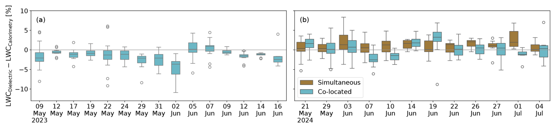
Figure 11 Bias between LWC measurements with dielectric devices and melting calorimetry for snow seasons of 2023 (a) and 2024 (b). In 2024, direct comparisons between simultaneous (brown) and co-located (light blue) measurements were also performed.

In Sect. 2.4, we explained how dielectric measurements were validated against melting calorimetry in conditions of ripe snow. We referred to the validation setup of 2023 as “co-located” only, whereas in 2024 we performed an additional “simultaneous” validation in addition to the co-located one. Figure 11 shows the spread between dielectric and calorimetric measurements in co-located and simultaneous setups for all the LWC validation measurements made over the 2 years. In 2023, the average maximum bias between co-located measurements is 2.6 % and the average standard deviation is 1.2 %. In 2024, the average maximum bias and the average standard deviation are 2.6 % and 1.4 % for co-located measurements and 2.3 % and 1.5 % for simultaneous measurements, respectively. Figure 13 shows all the measured vertical profiles in detail. In 2023, there is overall good agreement between dielectric and calorimetric measurements. The time lag between the measurements is highlighted by often similar LWC profile shapes, with calorimetry generally measuring higher peak values. Unexpectedly, in 2024, the simultaneous measurements resulted in only slightly lower biases and slightly higher standard deviations. This counterintuitive result is supported by a number of previous studies. For example, Donahue et al. (2022) found an average standard deviation of 1 % over 10 cm wide snow samples with LWC between 0 % and 5 %. The study of Techel and Pielmeier (2011) confirms the high occurrence of measurement deviations of more than 1 % at short horizontal distances. However, Techel and Pielmeier (2011) also show that the correlation between measurements at larger horizontal distances is higher for LWC values lower than 1.3 %. Therefore, the biases and standard deviations observed in our field measurements may overestimate the instrument uncertainty and/or variability over larger scales comparable to the footprint of S1. Based on these considerations, we define the large-scale LWC variability as ±1 %. We use this value to assess the effect of LWC uncertainty in ${\mathit{\sigma }}_{\mathrm{0}}^{\mathrm{VV}}$ retrievals from ground measurements.

4.3 Interpretation of Sentinel-1 backscatter through SMRT simulations forced by field measurements

Figure 12 shows the comparison between the time series of S1 acquisitions and SMRT-modelled ${\mathit{\sigma }}_{\mathrm{0}}^{\mathrm{VV}}$ forced by snow pit measurements using the two different permittivity formulations (MEMLSv3 and H-86) and the model setup described in Sect. 3.2, considering the LWC variability of ±1 % estimated in Sect. 4.2. In this figure, together with Table 3, simulation results are categorized into groups, and potential sources of inconsistencies and/or driving scattering mechanisms are discussed for each group, based on the measured values of LWC, TWC and surface roughness. All measured profiles of LWC, along with the corresponding TWC and RMSH values, are presented in Fig. 13 and Table 5, which serve as a reference for the following analysis. Table 4 shows all the root mean squared errors (RMSEs) between S1 acquisitions and simulations, according to the snow season, the selected permittivity formulation and the melting phase. In general, both models exhibit a mean negative bias of ≃ 5 dB with respect to S1 recordings over both seasons; however, biases are more pronounced for 2024 than for 2023, with the deviation between permittivity models being higher as well in 2024. H-86 generally gives higher ${\mathit{\sigma }}_{\mathrm{0}}^{\mathrm{VV}}$ values with respect to MEMLSv3.

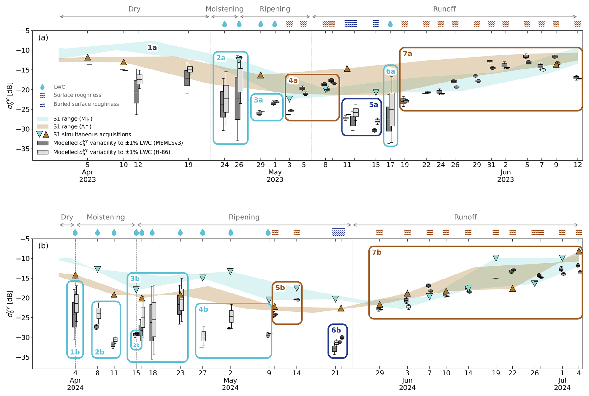
Figure 12 Comparison between the recorded multitemporal S1 ${\mathit{\sigma }}_{\mathrm{0}}^{\mathrm{VV}}$ (triangles and shaded areas) and the time series of ${\mathit{\sigma }}_{\mathrm{0}}^{\mathrm{VV}}$ modelled with SMRT, for the years 2023 (a) and 2024 (b). Results are shown for both permittivity formulations – MEMLSv3 (dark grey boxplots) and H-86 (light grey boxplots). The boxplots indicate the variability associated with the LWC uncertainty of ±1 % for each layer, as discussed in Sect. 4.2. The shaded areas of the recorded S1 multitemporal ${\mathit{\sigma }}_{\mathrm{0}}^{\mathrm{VV}}$ represent the range of values obtained by connecting the consecutive passages by the direction of orbits, i.e. by connecting all the morning/descending and the afternoon/ascending acquisitions. The triangles represent the exact values of the acquisitions. For clarity, exact values are only shown for days where snow measurements were carried out, thus allowing direct comparison. Coloured boxes group similar simulation results and are labelled with codes (e.g. 1a, 2a), which refer to Table 3 for details on the corresponding measured snow properties, dominant scattering mechanisms and potential sources of error. At the top of each panel, the time series are further segmented into the melting phases identified in Sect. 4.1 – as well as the main scattering regimes, which are influenced by LWC, surface roughness and buried surface roughness.

In 2023, the #066 morning S1 track recorded a backscatter increase of more than 2 dB between 5 and 19 April. Similarly, in 2024, we observe a 2.5 dB increase in backscatter recorded for track #117 from 8 February to 4 March. We can hypothesize that such increases are driven by the thawing of the soil. However, our data are insufficient and too uncertain to prove this because of possible interferences between dielectric instruments and the ground in mostly dry snow conditions, as mentioned in Sect. 2.1.4. In dry snow conditions, there were no significant discrepancies between S1 and simulations; hence Fig. 12 only focuses on the period after the assumed soil thawing.

Aside from the chosen permittivity formulation, five primary sources of uncertainty may account for the differences between simulated and recorded ${\mathit{\sigma }}_{\mathrm{0}}^{\mathrm{VV}}$. A significant one is snow transformation and melting between satellite and measurement acquisitions. S1 orbits intersect the field area either in the early morning or in the late afternoon (see Table 1). As explained in Sect. 2.4, measurements started at around 10:00 (UTC+1) and would take several hours. Thus, it is likely that in both cases the LWC during the passage is lower than the value measured at 10:00 (UTC+1) or later because of daily melt–refreeze cycles, especially near the snowpack surface. Moreover, the pointwise LWC measurements are not necessarily representative of the general liquid water distribution over the entire S1 cell. In 2023, we consistently observed ice layers over a high number of consecutive snow profiles (see Figs. 8c and 13). Our consecutive measurements suggest that ice layers contributed to creating a more spatially homogeneous liquid water distribution by acting as a natural drainage barrier for meltwater. Unlike in 2023, in 2024 ice layers were not consistently observed in the field. The melting process was likely more heterogeneous over the S1 cell, and pointwise measurements are less representative of wider scales in this season. This explains the fact that days marked by high variability associated with LWC are more numerous in 2024 than in 2023. In Table 3, we grouped these sources of uncertainties together under the label `uncertainty in spatiotemporal LWC/TWC”. Potentially, this source of uncertainty affects every S1 retrieval from field data. However, it definitely carries more weight than other sources of error at early melt stages when the simulation variability associated with LWC uncertainty is particularly high, i.e. when the TWC is low (24–26 April 2023, 4 April 2024) and during the cold spells of both 2023 (17 May) and 2024 (15–23 April), which caused the partial refreeze of the snowpack (see Figs. 8, 9b–d).

Daily melt–refreeze cycles, however, not only alter the amount of LWC/TWC in the snowpack, but also drive the formation of surface structures that can create additional scattering which is not accounted for in the simulations, i.e. crusts (Lund et al., 2022; Brangers et al., 2024). In Table 3, we labelled this uncertainty source as “scattering from surface structures (melt–refreeze)”. This uncertainty applies to the same cases as where “uncertainty in spatiotemporal LWC/TWC” applies, but it likely holds more weight when the TWC is slightly higher and the simulation variability according to LWC is lower (8–15 April 2024, 27 April–5 May 2024).

Another cause of significant discrepancy between recorded and modelled ${\mathit{\sigma }}_{\mathrm{0}}^{\mathrm{VV}}$ in the presence of a mostly dry snowpack with a smooth surface may be the thawing of the soil. This process creates a thin layer of liquid water overlying the natural soil roughness or absorbed into the basal snow layer (Lombardo et al., 2025). The combination of snow wetness and roughness, as will be shown later in the paper, can be responsible for backscatter increases up to 7 dB. In Table 3 we refer to this kind of uncertainty as “wet-soil scattering”. This uncertainty potentially applies to the instances when the TWC is relatively low and the variability associated with LWC is high. Between 4–27 April 2024, our measurements show considerable amounts of liquid water at the soil interface with otherwise relatively dry snowpack and smooth surfaces (see Fig. 13). The lysimeter time series corroborates these measurements by detecting runoff start on 8 April 2024 (see Fig. 9e). However, we lack sufficient data in order to prove and explore this possible scattering source; therefore we only mention it as a hypothesis.

Table 3 Supplementary information to Fig. 12: measured values of TWC, LWC and RMSH; noteworthy events for scattering (such as cold spells or late snowfalls); and explanations for the mismatch between modelled and recorded S1 backscatter signatures.

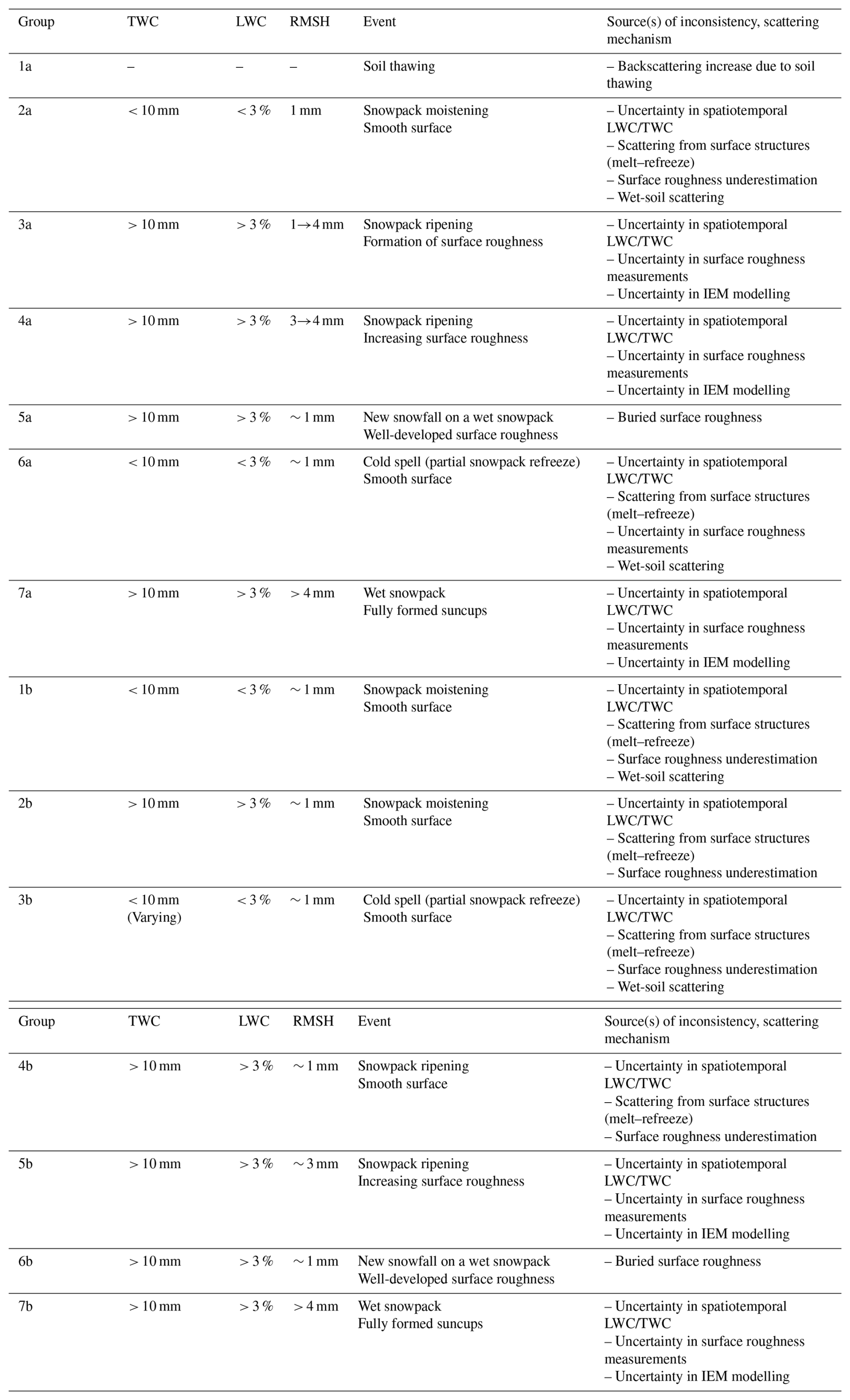
Table 4 RMSE (in dB) between modelled and recorded ${\mathit{\sigma }}_{\mathrm{0}}^{\mathrm{VV}}$ values according to the snow season, the selected permittivity formulation and melting phase.

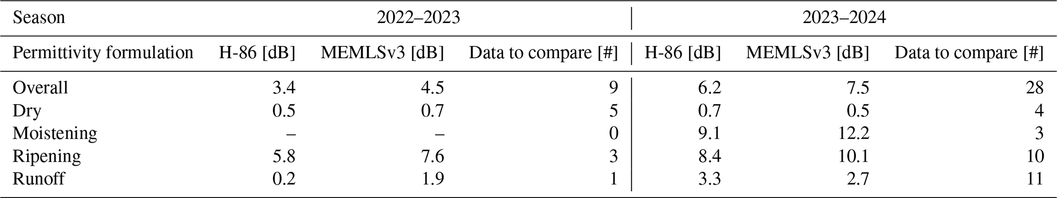
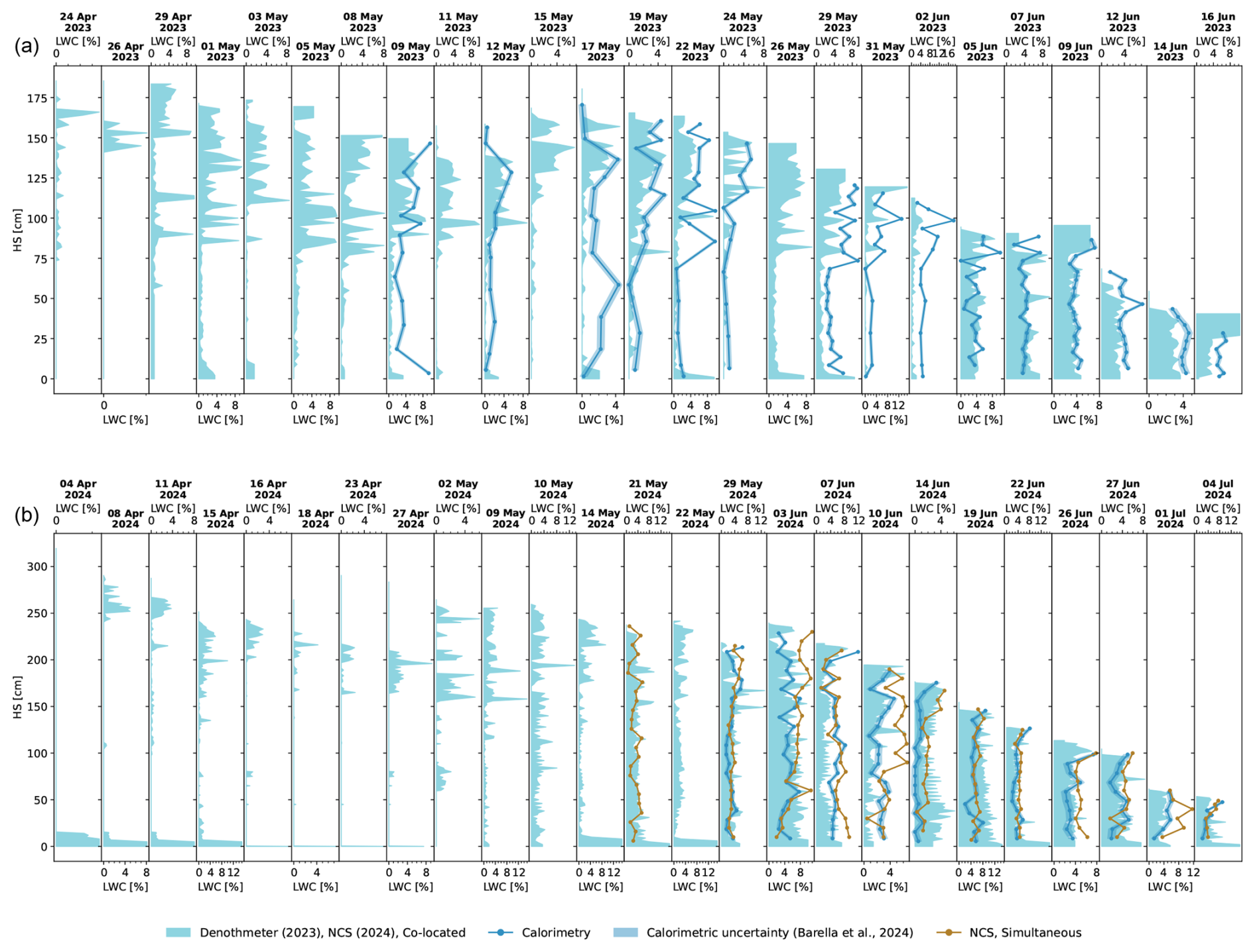
Figure 13 Ensemble of all the LWC profiles measured with dielectric instruments (light blue) from 24 April 2023 and 4 April 2024, i.e. the first dates for which there are significant mismatches between modelled and S1-acquired ${\mathit{\sigma }}_{\mathrm{0}}^{\mathrm{VV}}$ values in 2023 (a) and 2024 (b), respectively. Melting calorimetry measurements (dark blue), including their associated uncertainty (dark-blue shaded areas) as described in Barella et al. (2024), are shown for comparison. In 2024, a second simultaneous LWC profile using dielectric instruments (brown) was also obtained.

Table 5 Total water content (TWC) and surface roughness (RMSH) values measured for the LWC profiles shown in Fig. 13.

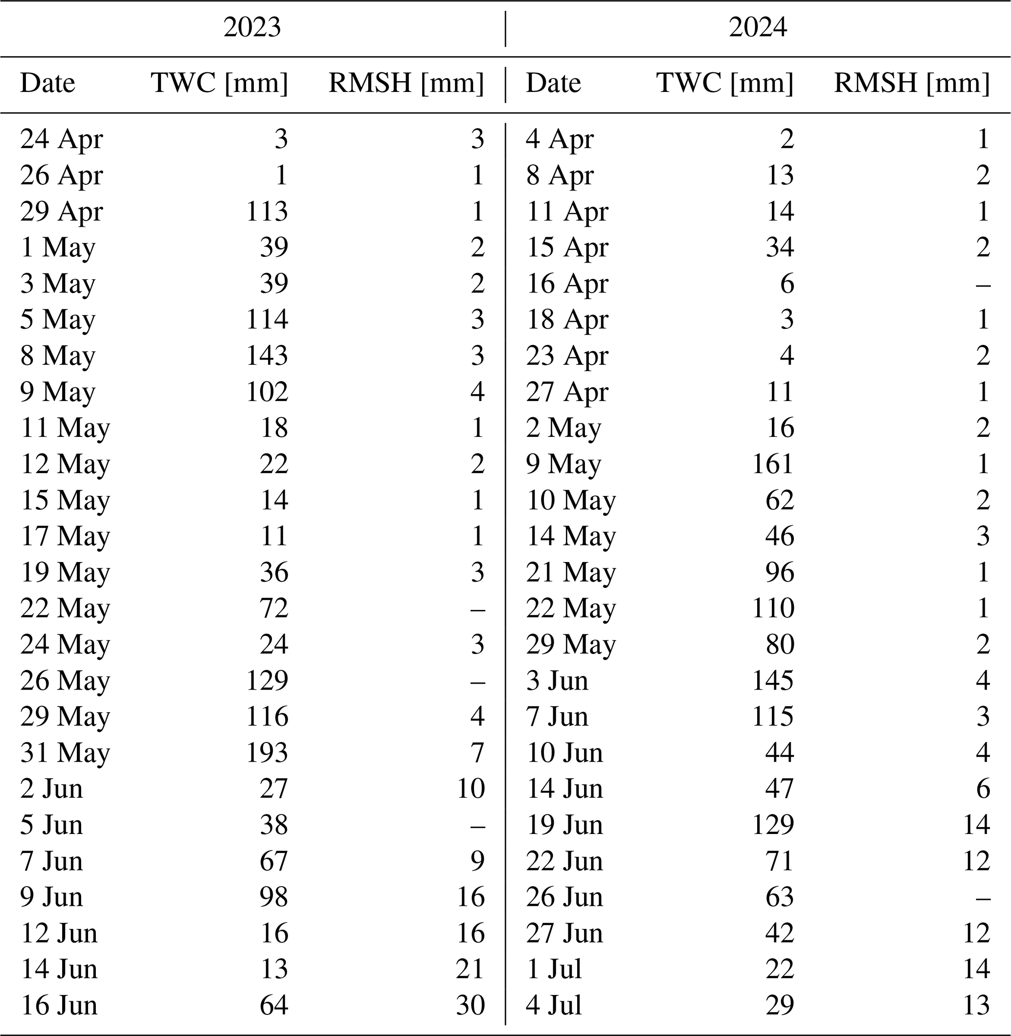
Two similar instances in 2023 (5–9 May) and 2024 (10 and 14 April) suggest another interesting phenomenon likely affecting simulation accuracy. In both these intervals, Fig. 12 shows very good agreement between recorded and modelled values of ${\mathit{\sigma }}_{\mathrm{0}}^{\mathrm{VV}}$, regardless of the chosen permittivity model and the variability associated with LWC. In both instances, surface roughness had just started developing on a wet-snow surface (LWC > 3 %), with measured RMSH values between 3 and 4 mm (see Fig. 10b). Thereafter, spring snowfalls cover the early-stage roughness and the snow surface reverts to smooth, with RMSH values between 1 and 2 mm (see Fig. 10a). In both years, the group of simulations following the spring snowfalls (i.e. 11–15 May 2023, 21 and 22 May 2024) again shows strong biases when compared to S1 recordings. This bias is almost certainly due to the fact that the surface roughness which had started to develop was then buried below a smooth layer of new snow, and it is not simulated by SMRT in the proposed configuration (see Sect. 3.2). In Table 3 we label this phenomenon “buried surface roughness”.

Generally, simulations are in better agreement with S1 recordings when the measured surface RMSH is above 3 mm. Figure 12 shows multiple groups of simulations where S1 retrievals from field data gain increasing accuracy with increasing RMSH on a wet surface, together with a decreasing dependence on the chosen permittivity model and the uncertainty associated with LWC (29 April to 9 May 2023, 19 May to 9 June 2023, 29 May to 1 July 2024). These instances suggest that in conditions of increasing surface roughness on a wet-snow surface, an additional source of uncertainty in S1 retrievals from field data might be associated with the IEM (see Sect. 3.2) translating surface roughness into backscatter response and/or with pointwise panel measurements underestimating the surface roughness of the entire S1 cell. In Table 3 we labelled these sources “uncertainty in IEM modelling” and “uncertainty in surface roughness measurements”, respectively.

Interestingly, the S1 signal is saturated at values of ${\mathit{\sigma }}_{\mathrm{0}}^{\mathrm{VV}}$ of −22.4 and −23.7 dB for 2023 and 2024, respectively. These values are close to the nominal noise-equivalent sigma naught (NESZ) of S1, i.e. −22 dB. The saturation of the signal is obtained by SMRT at much lower values, around ∼ −30 dB, regardless of the chosen permittivity formulation.

4.3.1 C-band radar backscatter sensitivity to the coupled evolution of surface roughness and liquid water content

To study the C-band radar backscatter sensitivity to the coupled evolution of surface roughness and LWC, we selected the date of 16 April 2024. On this date, we measured a melt event in the superficial 45 cm. The bottom part of the snowpack was homogeneously dry and was discretized as one layer with the average of the scattering properties measured in the field. These values are representative of a compacted snowpack structure at the beginning of the melt process: density of 428 kg m⁻³, SSA of 15.1 m² kg⁻¹ and temperature of −0.1 °C. From this configuration, we prepared a series of synthetic snowpack variations with surface LWC increasing from 0 % to 12 % and coupled each of them to a range of surface roughness RMSH values increasing from 1 to 15 mm. These extremes represent a smooth surface typical of recent snowfall and the highly textured surface of fully formed suncups, respectively. To ensure consistency, we gradually increased the value of the second roughness parameter CL as well. To do so, we used an empirical logarithmic relationship extracted from field data between RMSH and CL, which we report in Fig. A1. However, this empirical relationship is based on a limited number of points (75 in total) which show larger spread for increasing values of RMSH. Therefore, we assume that the only two discontinuities in the experimental results (see Fig. 14a–c, RMSH = 3 mm and LWC_top=12 %) can be explained considering this uncertainty. For clarity, these points were removed. All experiments were run with two incidence angles – 30 and 40° – which represent the overall range of angles between satellite overpasses and the snow surface within the reference cell (see Fig. 2 and Table 1). The result of all the experiments is shown in Fig. 14, for both permittivity formulations.

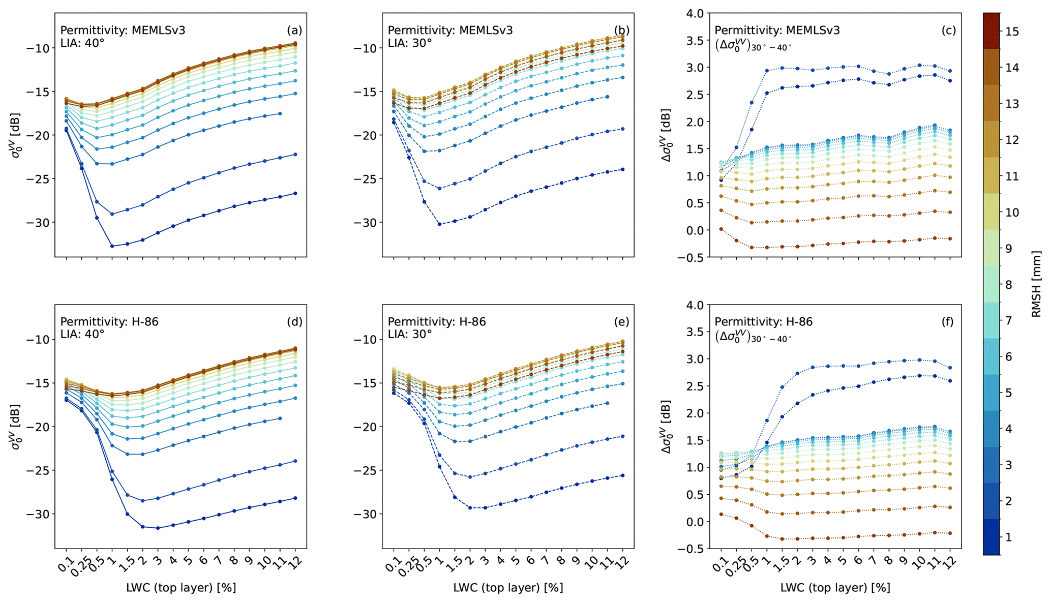
Figure 14 Sensitivity of the C-band radar backscatter to the coupled evolution of surface roughness (expressed by RMSH) and LWC. Panels (a), (b), (d) and (e) illustrate differences between two dielectric permittivity formulations – MEMLSv3 (a, b) and H-86 (c, d) – as well as the sensitivity to the local incidence angle (LIA) over cell 40. ${\mathit{\sigma }}_{\mathrm{0}}^{\mathrm{VV}}$ responses are shown for 40° (solid lines) and 30° (dashed lines) incidence angles. Panels (c) and (f) show values of ${\left(\mathrm{\Delta }{\mathit{\sigma }}_{\mathrm{0}}^{\mathrm{VV}}\right)}_{\mathrm{30}-\mathrm{40}\mathit{°}}$, i.e. the differences between backscatter coefficients in (b), (a) and (e), (d), respectively. The real reference case is the snowpack layering observed on 16 April 2024: a melt event in the superficial 45 cm and an otherwise dry snowpack. The reported results are consecutive synthetic variations of LWC and roughness of the surface layer.

In general, Fig. 14 shows that the intensity of the scattering response has a strong dependence on LWC for lower values of surface roughness (RMSH ≤ 3 mm). The higher the surface roughness, the weaker the dependence on LWC. In more detail, with H-86, for LWC values lower than or equal to 0.5 %, simultaneously increasing surface LWC and surface roughness causes a decrease in C-band ${\mathit{\sigma }}_{\mathrm{0}}^{\mathrm{VV}}$ of a maximum of 2 dB. Within this range, the intensity of the ${\mathit{\sigma }}_{\mathrm{0}}^{\mathrm{VV}}$ drop from smooth to rough surfaces decreases gradually with increasing LWC. For LWC values higher than 0.5 %, the spread in ${\mathit{\sigma }}_{\mathrm{0}}^{\mathrm{VV}}$ as a function of increasing surface roughness for the same value of LWC increases, with a reversed trend. Simultaneously increasing LWC eventually generates a ${\mathit{\sigma }}_{\mathrm{0}}^{\mathrm{VV}}$ increase for all the considered roughness values in this experiment. Interestingly, the higher the surface roughness, the lower the LWC value needed to invert the trend: for RMSH = 15 mm (typical of a textured snow surface where suncups are visible but also very close to the limit of validity of the IEM), ${\mathit{\sigma }}_{\mathrm{0}}^{\mathrm{VV}}$ starts to increase for LWC ≥ 1 %, whereas for RMSH = 3 mm, the ${\mathit{\sigma }}_{\mathrm{0}}^{\mathrm{VV}}$ only starts to increase for LWC ≥ 2 %. For LWC values higher than the threshold of 0.5 %, the surface roughness influences the C-band backscatter response to an extent that is comparable to the effect of LWC alone over a smooth surface. Similar considerations can be made for the experiments run with MEMLSv3, but as a consequence of the different absorption, the above-mentioned changes in ${\mathit{\sigma }}_{\mathrm{0}}^{\mathrm{VV}}$ trends happen for lower values of LWC. Furthermore, the experiments in Fig. 14 reveal that, regardless of the permittivity formulation, for relatively low values of LWC (≃ 1 %), a change in surface RMSH from 2 to 3 mm generates a remarkable increase of ≃ 6 dB in the backscatter response. In our field campaign, we typically measured roughness values in this range over snow surfaces undergoing the first cycles of melt–refreeze metamorphism. Interestingly, the value of 6 dB is very close to the average bias observed between S1 acquisitions and SMRT-modelled ${\mathit{\sigma }}_{\mathrm{0}}^{\mathrm{VV}}$ during the moistening and ripening phase (see Table 4). This supports the hypothesis that panel measurements may underestimate the large-scale surface roughness. Moreover, the backscatter increase occurring for all LWC and regardless of the incidence angle confirms that the monotonous increase in backscatter following the local minimum can be attributed to the formation of suncups, as initially suggested by the measurements alone.

Finally, Fig. 14c and f allow considerations regarding the impact of the incidence angle. To do so, we use the index ${\left(\mathrm{\Delta }{\mathit{\sigma }}_{\mathrm{0}}^{\mathrm{VV}}\right)}_{\mathrm{30}-\mathrm{40}\mathit{°}}$, i.e. the difference in backscatter between simulations at incidence angles of 30 and 40° – the range of incidence angles overlooking the reference cell. For smooth surfaces (1≤ RMSH ≤2) and for LWC ≥1.5 %, $\mathrm{\Delta }{\mathit{\sigma }}_{\mathrm{0}}^{\mathrm{VV}}$ exceeds 2 dB, i.e. twice the nominal uncertainty of S1 (see Sect. 2.3). For LWC lower than 1.5 %, $\mathrm{\Delta }{\mathit{\sigma }}_{\mathrm{0}}^{\mathrm{VV}}$ is highly sensitive to small increases in LWC. For RMSH ≥3, the sensitivity of $\mathrm{\Delta }{\mathit{\sigma }}_{\mathrm{0}}^{\mathrm{VV}}$ to changes in LWC almost disappears. In conditions of fully formed suncups (RMSH ≥10), $\mathrm{\Delta }{\mathit{\sigma }}_{\mathrm{0}}^{\mathrm{VV}}$ drops below the nominal sensitivity of 1.0 dB for every LWC value, meaning that the backscatter signals show progressively weaker angular dependence for highly structured snow surfaces. This phenomenon is easily understood considering that, on rough surfaces, diffuse scattering is enhanced. Therefore, the position of the sensor relative to the snow surface becomes less important, as the reflected energy is less directional and more broadly scattered. The same phenomenon explains the apparent slight backscatter decrease for RMSH ≥10 at angles of 30° (Fig. 14b, e). At lower incidence angles, the radar beam is closer to perpendicular to the surface than it is at higher incidence angles. On rough surfaces, with enhanced diffuse scattering, the fraction of energy reflected directly back to the sensor is reduced.

5 Discussion

Two consecutive years of detailed snow profiling with specific focus on the melting season gave an unprecedented overview of the multitemporal evolution of the SAR backscatter as a result of the changing snowpack properties. The identification of the melting phases from multitemporal SAR backscatter as proposed by Marin et al. (2020) was complicated by two factors: (i) the failure of Sentinel-1B in 2022, which halved the temporal coverage of satellite acquisitions, and (ii) lower incidence angles dampening the backscatter response to snow moistening. As a matter of fact, the optimal incidence angle for wet snow separability is approximately 45° (Nagler et al., 2016; Karbou et al., 2021), in line with the experimental results shown in Fig. 14. Despite these limitations, using nothing more than information on ${\mathit{\sigma }}_{\mathrm{0}}^{\mathrm{VV}}$ change with respect to winter means, the threshold-based method identified the moistening and ripening phases for both years with high accuracy.

With the first measured time series of surface roughness parameters, we demonstrated that for a high-altitude alpine snowpack – where radiation can be the dominant energy input during the melting season and surface roughness develops several weeks before the snow cover starts showing patches – the observed monotonous increase in backscatter at the end of the melting season is physically related to the development of surface roughness, from initial surface degradation due to melt–refreeze cycles and/or the sequence and intensity of snowfall events to the formation of suncups. This phenomenon was only hypothesized by Marin et al. (2020). Without ground-truth reference, it is impossible to distinguish the effect of surface roughness from disappearing snow using multitemporal SAR backscatter alone. Additionally, the start of the monotonous increase in multitemporal SAR backscatter defines the local minima in the time series. Several studies were carried out in recent years where such minima were associated with the runoff start (Gagliano et al., 2023; Darychuk et al., 2023). However, the proximity of the backscatter minimum and runoff start is not due to SAR direct detection of meltwater. Instead, this apparent coincidence arises at the specific frequency of S1 because of the interplay of several factors. As the snowpack reaches the maximum detectable water content by S1 (which reduces scattering), surface roughness begins to develop, enhancing scattering. These mechanisms will be discussed individually in the remainder of this discussion. Based on our data, the only and most likely conclusion we can draw from the backscatter minima from a practical point of view is that the snowpack is in an isothermal state and likely already releasing water. However, processes such as melt–refreeze cycles, sublimation, compaction or settlement in the upper snow layers can potentially lead to the formation of rough surfaces before the snowpack starts releasing meltwater runoff. Therefore, it is relevant to rethink how information on backscatter minima is used for hydrological applications, especially when counting on a limited satellite revisit frequency. Further research should also investigate other potential energy input mechanisms that are typical of snowpacks in environments outside the high-altitude and mid-latitude conditions explored in this study.

With radiative transfer modelling, we were able to link measured snow properties to retrieved satellite-based radar signals, aiming at reproducing the multitemporal backscatter time series recorded by S1. This analysis revealed that – rather than melting phases – the multitemporal S1 backscatter time series identify two main regimes, each driven by a different dominant factor influencing the radar response: LWC and surface roughness. Thus, as shown in Fig. 12, the moistening and ripening phases could be merged into a single phase primarily dominated by LWC, whereas the runoff phase could be redefined as a roughness-dominated phase. Modelling satellite backscatter signals forced by field measurements requires accounting for several sources of uncertainty, which are predominantly associated with these two variables. The uncertainty associated with LWC manifests itself in many different ways: the time lag between satellite and measurement acquisitions, the scattering originating from surface structures formed by melt–refreeze cycles, the spatial heterogeneity of the LWC distribution, the instrument uncertainty associated with the measurements, and, on the RT modelling side, a lack of a definite permittivity formulation for wet snow. The uncertainty associated with surface roughness is mostly linked to measurement inaccuracies (and/or non-representativeness for the entire S1 cell) and, on the RT modelling side, with possible errors in the IEM surface model.

Within the approximately 5 h separating satellite and measurement acquisitions, the liquid water per layer can change significantly (Kendra et al., 1998; Techel and Pielmeier, 2011), especially during the moistening and ripening phases or within cold spells, as indicated by the higher simulation variabilities in Fig. 12. In early stages of the melt process, our measurements are likely not representative of the snowpack state overlooked by S1 because of the strong effect of melt–refreeze. Our findings confirm that C-band ${\mathit{\sigma }}_{\mathrm{0}}^{\mathrm{VV}}$ is highly sensitive to diurnal snowpack variability, particularly during the early stages of melting when features such as melt–refreeze crusts are present (Lund et al., 2022; Brangers et al., 2024). As noted in Brangers et al. (2024), this strong dependence potentially complicates LWC retrievals significantly at these latitudes. This point raises concerns because the early stages of melting represent a critical period when S1 can detect LWC and likely the only window of opportunity to obtain and integrate reasonable information. However, our RT simulations forced by field measurements were able to attribute the observed ${\mathit{\sigma }}_{\mathrm{0}}^{\mathrm{VV}}$ drops across all tracks over both years – 6.2, 4.2, 1.5, and 7.8 dB – to corresponding measured TWC of 3, 1, 2, and 34 mm, respectively. These results are in line with the tower-based experiments of Strozzi et al. (1997) and Strozzi and Matzler (1998).

Another issue is the instrument uncertainty in LWC measurements. The deviations between dielectric and calorimetric measurements that we obtained throughout the campaign are in line with previous field and lab studies (Kinar and Pomeroy, 2015; Avanzi et al., 2016). Unexpectedly, co-located measurements in 2023 in the presence of ice lenses showed smaller deviations with respect to simultaneous measurements in 2024. Localized high values of LWC, such as for ponding meltwater above ice lenses, can pose accuracy problems for instruments that empirically estimate the volumetric liquid water content from the snow permittivity (Techel and Pielmeier, 2011). However, as previously noted, their presence could homogenize the overall liquid water distribution in the cell overlooked by the satellite. The increased variability between measurement techniques in 2024 may be (at least partially) due to the increased LWC heterogeneity compared to 2023. This may indicate that the snowpack stratigraphy and LWC conditions play a larger role than measurement errors due to spatial and temporal offsets. Accounting for the LWC instrument uncertainty – which we estimated to be approximately 1 % from our measurements, in line with previous similar comparative studies (Techel and Pielmeier, 2011; Donahue et al., 2022) – generates an uncertainty range in the simulated ${\mathit{\sigma }}_{\mathrm{0}}^{\mathrm{VV}}$ which is higher than the variability in the signal recorded by S1 over the course of one snow season. The highest deviations happen for the highest values of LWC, in line with the findings of Veyssière et al. (2019).

Finally, the lack of a definitive permittivity formulation for wet snow poses a significant challenge for the scientific community. The permittivity formulations selected for this study exhibit similar spectral shapes (see Fig. 5) and are, to our knowledge, the only ones validated against real-world observations at C-band frequencies. As mentioned in Sect. 3.2, the permittivity formulation describes how the real and imaginary parts of ϵ_s change with increasing fractions of liquid water and therefore how radar microwaves interact with the snowpack. ϵ_s is computed using mixing theories to account for volume fractions of ice, water and air in the snow medium. MEMLSv3 parametrizes the shape of water inclusions as elongated spheroids embedded in a homogeneous host medium. This represents an important source of uncertainty. As liquid water increases, the shape and orientation of water inclusions significantly affect ϵ_s, as the electromagnetic field interacts with them in a shape-dependent way, generating anisotropic responses (Arslan et al., 2003; Chang et al., 2016). However, characterizing the temporal evolution of the shape of water inclusions during melting processes is an ambitious and challenging task that was only recently addressed by Krol et al. (2024) through rapid MRI profiling in a controlled laboratory environment. At the time our measurement campaign was designed and conducted, these methods – let alone their applicability in the field, which is still entirely unknown – did not yet exist. These recent advancements are highly promising for the crucial challenge of developing a comprehensive model applicable across all frequencies and LWC conditions. Moreover, Fig. 12 highlights discrepancies of approximately 6 dB between SMRT-simulated and satellite-recorded backscatter signals, especially when ${\mathit{\sigma }}_{\mathrm{0}}^{\mathrm{VV}}$ is largely dominated by LWC. Similar deviations were found by Veyssière et al. (2019) using MEMLS&a to reproduce ${\mathit{\sigma }}_{\mathrm{0}}^{\mathrm{VV}}$ during consecutive melt seasons over alpine areas. Additionally, both permittivity models saturate ${\mathit{\sigma }}_{\mathrm{0}}^{\mathrm{VV}}$ at values below −30 dB. Such low values are never recorded by S1, which saturates ${\mathit{\sigma }}_{\mathrm{0}}^{\mathrm{VV}}$ at around −22 dB. The tower-based radiometric studies by Strozzi et al. (1997) and Strozzi and Matzler (1998) confirm signal saturation in the C-band vertical co-polarization at values between −20 and −25 dB. Matching the recorded S1 ${\mathit{\sigma }}_{\mathrm{0}}^{\mathrm{VV}}$ would require an imaginary part of ϵ_s similar to that at 1 GHz – this would imply unrealistic penetration depths for the C-band, contradicting field observations (Ulaby and Stiles, 1981; Shi and Dozier, 1995; Ulaby et al., 2014; Lodigiani et al., 2025). We conclude that one possible explanation for the observed deviations is the overestimated absorption loss in the existing permittivity formulations. In view of the described inherent limitations of such formulations, a detailed quantitative analysis of scattering contributions from individual snow layers was not possible. As noted in Sect. 3.2, the absence of a unified permittivity model for wet snow remains an important direction for future research – not only for RT modelling, but also for field measurements, since dielectric methods depend on such models to derive LWC.

Later in the melting season, the effects of the uncertainties associated with LWC become weaker because the snowpack surface becomes wetter and the scattering is mostly dominated by surface effects (Shi and Dozier, 1992) – this can be observed in Fig. 12, as variability associated with LWC decreases gradually with time. Simultaneously, deviations between modelled and recorded ${\mathit{\sigma }}_{\mathrm{0}}^{\mathrm{VV}}$ decrease substantially (groups 4a and 5b in Fig. 12 and Table 3). Here, deviations are most probably explained by inaccurate surface roughness quantification. This is particularly evident in instances where simulation accuracy drops after a spring snowfall on a surface that had already begun developing marked roughness (groups 5a and 6b in Fig. 12 and Table 3). However, at these later stages of the melting process, simulations reproduce the recorded backscatter generally well (groups 7a and 7b in Fig. 12). This is confirmed by the low RMSE values reported in Table 4 for the runoff phase, which we redefined as a phase dominated by surface roughness effects. Here, further deviations can be attributed to panel measurements possibly not fully capturing the large-scale roughness features observed by the satellite. This hypothesis seems to be confirmed by the very recent results of Barella et al. (2025), showing that panel sizes practical for field measurements may be insufficient to capture the roughness features of wider areas. Additionally, the IEM, which translates roughness parameters into scattering, could be affected by inaccuracies, especially when the roughness values approach or exceed the model's range of validity.

In other words, with Fig. 12, we tried to reproduce the recorded S1 ${\mathit{\sigma }}_{\mathrm{0}}^{\mathrm{VV}}$ over a 20×20 m cell using physics-based averages of fine, detailed snow properties measured at the point scale. At wider scales, the relative importance of very specific information on the state of the snowpack may decrease compared to more influential large-scale scattering drivers, namely the development of internal snowpack structures (e.g. ice lenses and crusts), the soil features in the case of an isothermal but predominantly dry snowpack and large-scale surface roughness. Although the modularity and comprehensiveness of SMRT theoretically allow most of these scenarios to be modelled, the problem of how to quantify them on a large scale persists.

In Fig. 14, we selected realistic snowpack layering observed in the field and used the full range of measured values of surface roughness to repeat the experiments done in the past by Shi and Dozier (1992), Strozzi et al. (1997), and Strozzi and Matzler (1998). These simulations aimed to characterize the scattering response of a wet-snow cover to increasing surface roughness while varying the incidence angle to match the range observed across the relative S1 orbits covering the study area. Since the relationship between co-polarized signals and snow wetness is controlled by the scattering mechanisms, the type of correlation between superficial LWC and surface roughness expresses the relative contribution of volume rather than surface scattering mechanisms (Shi and Dozier, 1992). Shi and Dozier (1992) found negative correlations with surface roughness for LWC between 2 % and 4 % and a positive correlation with increasing surface wetness at an incidence angle of 50°. Similar results were also found by Ulaby and Stiles (1981) at frequencies of 8.6 GHz and incidence angles greater than 50°. Our results generally confirm these findings, but the wider range of explored combinations of surface roughness and LWC reveals that the correlation tilt does not occur at a specific LWC value. For RMSH values (simply “roughness” hereafter) between 2 and 10 mm, typical of snow during most of the melting period, the tilt depends on both LWC and roughness, shifting towards higher LWC with lower roughness. Specifically, backscatter strongly depends on roughness when LWC values are equal to or exceed 3 %. Again, for smooth surfaces (1–2 mm), both permittivity models saturate ${\mathit{\sigma }}_{\mathrm{0}}^{\mathrm{VV}}$ below −30 dB, a value never recorded by S1.

An interesting result from Fig. 12 and Table 3 is that the most accurate simulations of S1 recordings happen when measured values of surface roughness equal or exceed the threshold value of 3 mm. The experimental analyses in Fig. 14 show that, for relatively low values of LWC between 1 % and 1.5 %, the backscatter response increases by approximately 6 dB when the roughness increases from 2 to 3 mm. The value of 6 dB is almost exactly the bias we observed in Fig. 12 between S1 recordings and our simulations, especially with increasing LWC. As mentioned, similar deviations were found by Veyssière et al. (2019). Additionally, for LWC values ≥ 1.5 % and roughness between 3 and 4 mm, the simulated ${\mathit{\sigma }}_{\mathrm{0}}^{\mathrm{VV}}$ is saturated at values that are comparable to those recorded by S1. This raises the point that more representative estimates of surface roughness for the entire S1 cell and/or improved IEM modelling to translate this information into backscatter signals could be just as crucial as rigorous permittivity formulations for accurately reproducing and better interpreting multitemporal S1 ${\mathit{\sigma }}_{\mathrm{0}}^{\mathrm{VV}}$. Recent findings by Barella et al. (2025) also point in this direction, suggesting that commonly used transect extraction algorithms may filter out some small-scale roughness features. In general, the experiments in Fig. 14 represent a substantial advancement with respect to Shi and Dozier (1992), Strozzi et al. (1997), and Strozzi and Matzler (1998). In these earlier experiments, surface roughness was either not quantitatively measured (being only qualitatively assessed) or evaluated over a very limited set of scenarios, overlooking intermediate conditions that, as our measurements prove, characterize the majority of the melting period.

Figure 14c and f show that for smooth surfaces and for LWC values as low as 1.5 % – i.e. when the melting process is likely in its initial stage – the variation in backscatter across the range of incidence angles overlooking the reference cell is comparable to or even exceeds the threshold used in Nagler and Rott (2000), Nagler et al. (2016), and Marin et al. (2020) for wet-snow detection. This angular dependence constitutes an additional uncertainty factor in wet-snow detection, which overlaps with the previously discussed effects of diurnal variability in snowpack properties. On the other hand, for LWC values higher than 2 % on smooth surfaces, the angular dependence increases up to 3 dB. This result supports the hypothesis that two distinct scattering mechanisms observed across the two seasons are directly linked to incidence angle effects. The first is a persistent 3–5 dB difference in ${\mathit{\sigma }}_{\mathrm{0}}^{\mathrm{VV}}$ between the two ascending tracks, recorded from mid-April to early June 2023 (see Fig. 8a). This spread was not observed in the following year. Our LWC measurements indicate that the snowpack surface was wetter in 2023 than in 2024, likely due to the presence of ice lenses acting as drainage barriers for meltwater and favouring the formation of a wetter layer above them (see Fig. 13 and Table 5). Consequently, and in line with the results in Fig. 14, the smoother and wetter snow surface in 2023 led to a stronger angular dependence compared to 2024. Additionally, the angular dependence decreases with increasing surface roughness. The second observed feature is the sharp decrease in backscatter between consecutive acquisitions of both ascending and descending tracks in 2024 – from 15 to 22 June and from 19 to 26 June, respectively. Our measurements indicate conditions of high snowpack saturation and surface roughness values equal to or exceeding 10 mm (see Fig. 13 and Table 5). Consistent with the results shown in Fig. 14b and e, we interpret this decrease as the result of suncup formation on a saturated snow surface. The enhanced surface roughness likely increased diffuse scattering and reduced the proportion of energy reflected back to the sensor, thereby explaining the observed backscatter decrease. These findings indicate that, despite all the aforementioned challenges in deriving LWC from backscatter and vice versa, the multitemporal analysis of angular dependence may carry valuable additional information. Unfortunately, further analysis in this direction was limited by the reduced revisit frequency of S1 during the period of this study.

Ultimately, Fig. 14 suggests that with an estimate of the surface LWC from a detailed snow model and recorded values of S1 backscatter, it is in principle possible to estimate surface roughness. This would give information on two interesting points. On the one hand, based on the position with respect to the curve tilt, it would be possible to have information about the dominance of the volume versus surface scattering mechanism. A prevalence of volume scattering would mean that the snowpack has not yet become a complete blackbody for C-band radar backscatter. On the other hand, the value of surface roughness could be assimilated in physics-based snow models to estimate important metrics for the computation of turbulent heat fluxes, such as the aerodynamic roughness length (Lehning et al., 2011).

Although promising for future research, this paper comes with a number of limitations. LWC is a key variable for interpreting and reproducing S1 acquisitions using radiative transfer models. However, despite ongoing advancements, accurately measuring LWC in the field, modelling it within physics-based snow models, and accounting for it in permittivity and RT models remain significant challenges which need to be solved individually. The halved availability of satellite data acquisitions due to the failure of Sentinel-1B in the exact time span when this study was carried out hindered the possibility of obtaining more information than that presented on the relationship between melting snowpack properties and the multitemporal SAR backscatter. Finally, despite this study significantly enhancing our understanding of the interaction of SAR backscatter with wet snow, our findings are likely valid for high-alpine regions, i.e. homogeneously covered by a rather high amount of snow, and where surface roughness can develop before the snow cover disappears in patches. The full capabilities of the Sentinel-1 mission will shortly be restored following the recent launch of the Sentinel-1C satellite. This development will hopefully spark greater interest in the field, driving research efforts to address the above-mentioned limitations, explore scattering mechanisms in environments other than the one explored in this study and potentially establish a new role for radiative transfer modelling – specifically, to inform physics-based snow models for hydrological applications.

6 Conclusions

In this paper, we presented a unique dataset of wet-snow scattering properties collected at a fine vertical and temporal resolution over two snow seasons at the high-alpine field site of Weissfluhjoch, Davos, Switzerland. Using this dataset, we analysed the correlation between melting snow properties and multitemporal SAR backscatter from S1 and modelled the satellite signals using the radiative transfer model SMRT. Our data show that the moistening and the ripening phase, being mostly related to the presence of liquid water in the snowpack, are generally well identified using time series of multitemporal SAR backscatter from S1. The runoff onset, often associated with local minima in multitemporal SAR backscatter, is not detectable by the satellite. With our measurements, we showed that these local minima result from a combination of surface wetting, which reduces backscatter until the S1 signal is saturated, and the development of surface roughness before the snow cover begins to disappear in patches, leading to an increase in backscatter. Therefore, it is important to rethink how this information is used for hydrological applications at high elevations and mid-latitudes, especially when counting on reduced satellite revisit times. Then, we used our dataset as input to the SMRT model to reproduce the S1 backscatter signal. The simulations generally showed a negative bias with respect to satellite acquisitions, with the most significant drivers being LWC in earlier stages of the melting process and the surface roughness later on. This mismatch led to the insight that, rather than melting phases, the multitemporal S1 backscatter time series reveal two dominant scattering regimes: one dominated by LWC and the other by surface roughness. These two regimes also represent the main sources of uncertainty in electromagnetic modelling of melting snowpacks. These challenges include the spatial and temporal variability of LWC between field measurements and satellite overpasses, inaccuracies in surface roughness estimation, and limitations in the permittivity and roughness models applicable to wet snow in the C-band. Despite these uncertainties, radiative transfer modelling driven by ground measurements allowed the in-depth physical interpretation of scattering mechanisms at different stages. Specifically, the unprecedented time series of measured surface roughness parameters allowed exploring and defining the scattering effect of roughness over wetting snowpacks at different incidence angles. Our findings suggest that accurately quantifying surface roughness and/or improving the transfer function in IEM modelling could be as critical as developing new, rigorous permittivity formulations to enhance S1 retrievals and our understanding of scattering mechanisms on wet snow at these wavelengths. With improved process understanding, the imminent restoration of the full capabilities of the S1 mission, and further validation of radiative transfer sub-modules, the use of C-band satellite radar signals in snow hydrology applications could proceed further, with radiative transfer models informing physics-based snow models.

Appendix A

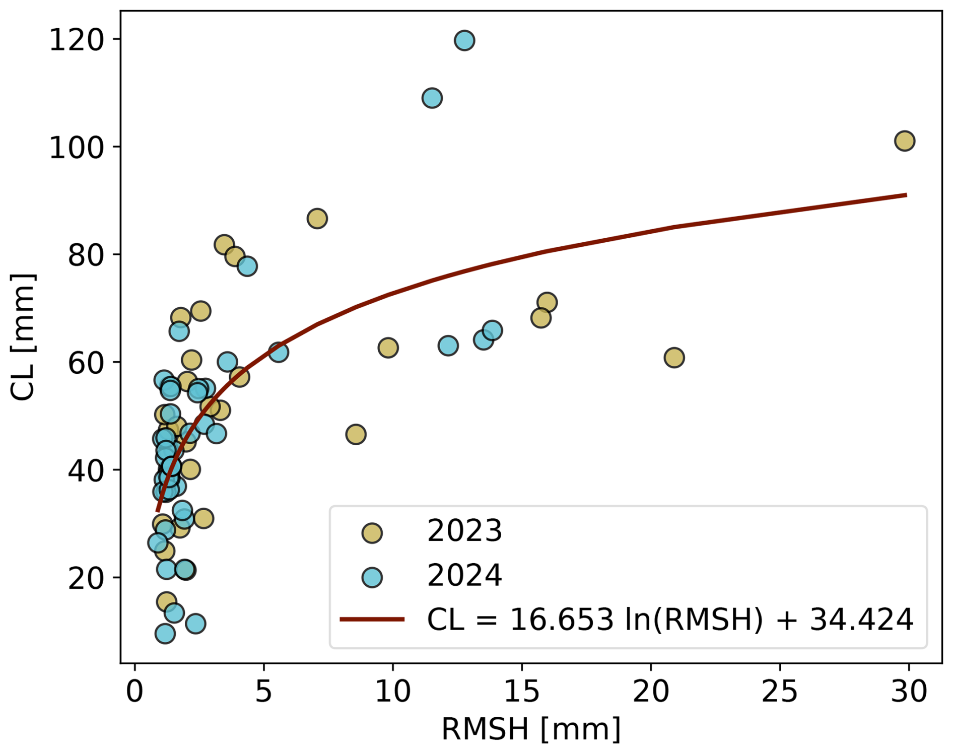
Figure A1 Empirical logarithmic relationship fitted on field data between the surface roughness parameters of RMSH and CL, based on a total of N=75 values over the measurement campaigns of 2023 (yellow) and 2024 (light blue).