ISMIP6-based Antarctic projections to 2100: simulations with the BISICLES ice sheet model

The contribution of the Antarctic Ice Sheet is one of the most uncertain components of sea level rise to 2100. Ice sheet models are the primary tool for projecting future sea level contribution from continental ice sheets. The Ice Sheet Model Intercomparison for the Coupled Model Intercomparison Phase 6 (ISMIP6) provided projections of the ice sheet contribution to sea level over the 21st century, quantifying uncertainty due to ice sheet model, climate model, emission scenario, and uncertain parameters. We present simulations following the ISMIP6 framework with the BISICLES ice sheet model and new experiments extending the ISMIP6 protocol to more comprehensively sample uncertainties in future climate, ice shelf sensitivity to ocean melting, and their interactions. These results contributed to the land ice projections of Edwards et al. (2021), which formed the basis of sea level projections for the Sixth Assessment Report of the Intergovernmental Panel on Climate Change (AR6). Our experiments show the important interplay between surface mass balance processes and ocean-driven melt in determining Antarctic sea level contribution. Under higher-warming scenarios, high accumulation offsets more ocean-driven mass loss when sensitivity to ocean-driven melt is low. Conversely, we show that when sensitivity to ocean warming is high, ocean melting drives increased mass loss despite high accumulation. Overall, we simulate a sea level contribution range across our experiments from 2 to 178 mm. Finally, we show that collapse of ice shelves due to surface warming increases sea level contribution by 25 mm relative to the no-collapse experiments, for both moderate and high sensitivity of ice shelf melting to ocean forcing.

1 Introduction

The Antarctic and Greenland ice sheets were the third-largest contributor to global mean sea level (GMSL) change from 1901 to 2018 behind thermosteric changes and mountain glaciers (Palerme et al., 2017; Horwath et al., 2022; Fox-Kemper et al., 2021), which together accounted for 79 % of the 20 cm of sea level rise (Fox-Kemper et al., 2021). In recent decades, ice sheet mass loss has contributed a growing proportion of sea level rise, which averaged 3.64 ± 0.26 mm yr⁻¹ between 2003 and 2016 (Horwath et al., 2022). From 1992 to 2020, the Antarctic Ice Sheet (AIS) contributed 7.4 ± 1.5 mm to global mean sea level rise (Otosaka et al., 2023). Although Antarctica was a smaller source of GMSL between 1993 and 2016 than other land ice sources and land water storage (Horwath et al., 2022), evidence of past volume and dynamics suggests that the ice sheet could become a significant source of GMSL in a warming climate (DeConto et al., 2021; Lowry et al., 2021; Edwards et al., 2019). To date, mass loss in Antarctica has been dominated by the dynamic glacier response to warm ocean currents eroding ice shelves in the Amundsen Sea sector (Shepherd et al., 2018; Rignot et al., 2019), with changes in ocean currents linked to anthropogenic-warming-driven changes to wind regimes (Holland et al., 2019). Along with some East Antarctic basins, the West Antarctic Ice Sheet may be vulnerable to ocean-driven instabilities as grounding lines retreat into over-deepened subglacial basins (Schoof, 2012; Weertman, 1974; Thomas, 1979). Around 23 m of sea level equivalent Antarctic ice rests on bedrock below sea level (Morlighem et al., 2020).

Under anthropogenic warming, ice loss from marine basins could drive accelerating GMSL contribution in coming decades to centuries (Schlegel et al., 2018; Bulthuis et al., 2019; Lowry et al., 2021; Edwards et al., 2019; DeConto and Pollard, 2016; Golledge et al., 2015; Ritz et al., 2015; Seroussi et al., 2024), with uncertainty around unstable marine ice retreat contributing to uncertainty in future sea level projections (Robel et al., 2019). Alongside this ocean-driven retreat under anthropogenic warming, increased Antarctic snowfall accumulation, particularly over East Antarctica, has the potential to mitigate the ice sheet's sea level contribution. Warmer air temperatures over Antarctica can increase precipitation, driving increased surface mass balance under the cold, low-melt conditions of the ice sheet (Frieler et al., 2015; Palerme et al., 2017). Over the course of the 20th century, increased precipitation offset ∼ 10 mm of AIS-sourced GMSL (Medley and Thomas, 2019).

Ice sheet models are the primary tool for projecting future Antarctic sea level contribution. Over the past few decades, models have developed to represent a greater range of ice sheet processes and climate–ice sheet interactions at higher resolution than ever before (Pattyn et al., 2017). However, differences in process representation, model physics, spatial discretisation, and initialisation (Seroussi et al., 2019) mean that different ice sheet models project different AIS responses to the same climate boundary conditions (Edwards et al., 2014; Bindschadler et al., 2013). The Ice Sheet Model Intercomparison Project for the Coupled Model Intercomparison Projects Phase 6 (CMIP6), ISMIP6 (Nowicki et al., 2016), builds on previous multi-model ensemble efforts (e.g. Edwards et al., 2014; Bindschadler et al., 2013) to better characterise uncertainty in projected future GMSL from the Greenland and Antarctic ice sheets (Nowicki et al., 2016). With a common set of experiments run by different modelling groups, it allows for improved quantification of uncertainty in sea level projections due to choice of ice sheet model.

Results of ISMIP6 Antarctic Ice Sheet experiments forced with Coupled Model Intercomparison Project Phase 5 (CMIP5) climate models are described by Seroussi et al. (2020), who find a range of −7.8 to 30.0 cm sea level equivalent (SLE) contribution from Antarctica between 2015 and 2100 under a very high-emission scenario (RCP8.5) compared with experiments under constant climate conditions. Under a low-emission scenario (RCP2.6), an average additional mass loss of 0.0 to 3.0 cm is found based on two CMIP5 models compared with simulations under modern climate (Seroussi et al., 2020). Comparing these results with a further ensemble of simulations using next-generation CMIP6 climate model forcings, Payne et al. (2021) find a limited difference between projections grouped by generation of CMIP climate model. This is attributed to the complexity of interactions between the AIS and the climate system, with warming-linked surface mass balance increases offsetting ocean-melt-driven mass loss in some cases (Payne et al., 2021). While CMIP6 models generally simulate more warming than CMIP5 models, both ocean melting and surface mass balance are enhanced in CMIP6, meaning that sea level contribution does not differ significantly by CMIP generation (Payne et al., 2021).

BISICLES ISMIP6 Antarctic experiments were used in the ISMIP6 synthesis and sensitivity tests of Edwards et al. (2021). However, with the exception of experiments for the model initialisation intercomparison exercise (InitMIP) (Seroussi et al., 2019), ISMIP6 BISICLES simulations have not yet been presented in detail (Edwards et al., 2021). We chose BISICLES to complement the original ISMIP6 ensemble experiments because of its use of adaptive mesh refinement and the L1L2 flow approximation (Cornford et al., 2013), making it well suited to simulating marine ice sheets (Cornford et al., 2015, 2016, 2020). This allows BISICLES to capture grounding line dynamics at high resolution and maintain computational efficiency.

We present here a set of 19 simulations (18 projections and a control) from the BISICLES ice sheet model following the ISMIP6 design for future projections of the Antarctic Ice Sheet. Our simulations follow the design for Tier 1, 2, and 3 experiments (Nowicki et al., 2016). Tier 1 are core ISMIP6 experiments using climate forcing derived from the highest skill models identified in Barthel et al. (2020) and exploring scenario dependence and sensitivity to shelf collapse and ice shelf basal melt sensitivity (Nowicki et al., 2016). Tier 2 experiments explore a wider range of models assessed in Barthel et al. (2020) from the CMIP5 ensemble and CMIP6 models based on availability. Tier 3 experiments provide a more in-depth exploration of the role of ocean sensitivity in modelled AIS evolution to complement Tier 1 (Nowicki et al., 2016).

We also explore the relationship between ocean melt and ice shelf collapse through additional sensitivity experiments. The Tier 1–3 experiments contribute to the ISMIP6 effort by adding another Antarctic Ice Sheet model to the ensemble, while the additional sensitivity experiments target uncertainties in the synthesis of Edwards et al. (2021) by testing for interactions between uncertain parameters.

Here we present the BISICLES model set-up and experimental design (Sect. 2) and results of the 19 ice sheet model experiments (Sect. 3). We then discuss the role of different modelling choices on Antarctic contribution to sea level, compare BISICLES to other ISMIP6 ice sheet models, and finally discuss limitations of our approach (Sect. 4).

2 Methods

2.1 BISICLES

BISICLES is a block-structured, finite-volume, ice sheet model solving the L1L2 flow approximation with adaptive mesh refinement (Cornford et al., 2013, 2015, 2016) (Supplement Sect. 1.1). For these simulations, we use the BISICLES_B model set-up as in Seroussi et al. (2019) and the same initial state. All simulations are run with a base resolution of 8 km, with three levels of refinement to reach a finest mesh resolution of 1 km (Supplement Fig. S1). The model domain at the coarsest level covers a grid of 768 × 768 cells. We use the sub-grid friction interpolation scheme described in Cornford et al. (2016). This allows for a finest resolution of 1 km at the grounding line and in regions of fast-flowing ice, adequately capturing grounding line dynamics compared with higher-resolution simulations where the sub-grid friction scheme is not used (Cornford et al., 2016).

Basal sliding is calculated using a pressure-limited Weertman–Coulomb type law (Tsai et al., 2015) with $m=\mathrm{1}/\mathrm{3}$ and a Coulomb friction coefficient of 0.5. This sliding law accommodates regions of hard beds and slow flow through the Weertman law, regions of faster flow on deformable beds through the Coulomb law, and a smooth transition between the two (Supplement Sect. 1.1, Eq. 6). Basal traction coefficients and the effective viscosity coefficient (ϕ) are estimated using an inversion approach to minimise the mismatch between modelled ice velocity and observations collected between 2007 and 2010 (Cornford et al., 2015) and are held constant throughout the simulations. Ice temperature is from Pattyn (2010), who simulated ice sheet temperature with a 3D thermomechanical ice sheet model, and it is fixed throughout the simulations. While BISICLES uses a depth-integrated momentum balance equation, the rate factor A(T) in effective viscosity is based on 3D ice temperature (Supplement Sect. 1.1, Eq. 5). The inverted parameter ϕ corrects the vertically integrated effective viscosity in essentially the same way as a damage parameter D (phi = 1 − D) (Supplement Sect. 1.1, Eq. 3) but will conflate the influence of errors in the ice temperature and thickness and the form of the rate factor. In the experiments presented here, the calving front is fixed, with the exception of “collapse on” experiments, where the ice shelf is removed based on collapse masks (see Sect. 2.2). However, floating ice thinner than 10 m is automatically calved. All simulations are initialised from a 9-year relaxation run, as in previous BISICLES studies (Cornford et al., 2016) (Supplement Sect. 1.3). While the ISMIP6 analysis period is from 2015 to 2100, our simulations start in 2010 and use the ISMIP6 forcing anomalies provided, which cover the period 1995–2100.

Ice sheet contribution to sea level is calculated from the change in ice volume above floatation (VAF) in the absence of bedrock deformation, which is a process we do not include. Volume above floatation is the volume of ice sheet that is not below sea level or hydrostatic equilibrium and is therefore not already displacing ocean water. To calculate sea level contribution, i.e. the change in VAF in metres sea level equivalent (m s.l.e.) for the modern ocean, we distribute sea level equivalent change in VAF over an ocean area of 3.625 × 10¹⁴ m² (Gregory et al., 2019) that has an ocean water density of 1028 kg m⁻³ and an ice density of 918 kg m⁻³ (Goelzer et al., 2020). As we use an inversion approach, some retreat in our model is due to dynamic retreat not driven by climate, which is nonetheless an important component of the ice sheet's future sea level contribution. We therefore present our results without subtracting the control sea level contribution.

2.2 Ocean and atmosphere forcing

We use the three models identified in Barthel et al. (2020) as having the highest skill in simulating climate variables and sample a diverse subset of CMIP5 climate models. These are NorESM1-M, CCSM4, and MIROC-ESM. Additionally, we use one CMIP6 model in our simulations, CNRM-CM6-1, as forcing data were available to us for both low-emission (SSP1-2.6) and high-emission (SSP5-8.5) scenarios, which was not the case for other CMIP6 models. We can therefore explore scenario dependence across a wider range of GCMs (general circulation models) and across CMIP generations.

To promote a consistent approach to basal melt forcing across ice sheet models, most participating groups used a prescribed basal melt parameterisation (Jourdain et al., 2020; Nowicki et al., 2020). This parameterisation describes the relationship between basal melting, m, and ocean thermal forcing, TF. BISICLES implements the “non-local” basal melt rate parameterisation. Basal melt anomalies, relative to the initial melt forcing, are applied for each simulation year. The non-local basal melt parameterisation captures the melt-induced cavity-scale circulation changes that drive shelf melt (Jourdain et al., 2017) and the local influence of stratification and compares favourably to coupled ice sheet ocean models in idealised experiments (Favier et al., 2019). A more comprehensive description can be found in Jourdain et al. (2020). It is restated here:

$$\begin{array}{}\text{(1)}& \begin{array}{rl}m(x,y)=& {\mathit{\gamma }}_{\mathrm{0}}\times {\left({\displaystyle \frac{{\mathit{\rho }}_{\mathrm{sw}}{C}_{\mathrm{pw}}}{{\mathit{\rho }}_{\mathrm{i}}{L}_{\mathrm{f}}}}\right)}^{\mathrm{2}}\\ & \times \left(\mathrm{TF}\right(x,y,z_{\mathrm{draft}})+\mathit{\delta }{T}_{\mathrm{sector}})\\ & \times |\langle \mathrm{TF}{\rangle }_{\mathrm{draft}\in \mathrm{sector}}+\mathit{\delta }{T}_{\mathrm{sector}}|,\end{array}\end{array}$$

where ρ_i and ρ_sw are the densities of ice (918 kg m⁻³) and seawater (1028 kg m⁻³), respectively; L_f is the fusion latent heat of ice (3.3 × 10⁵ J kg⁻¹); and C_pw is the specific heat of seawater (3974 J kg⁻¹ K⁻¹). The thermal forcing, TF, is calculated at the ice–ocean interface, while 〈TF〉 is averaged over each of the 16 Antarctic sectors. Figure 1 shows thermal forcing averaged over the surface ocean (0–500 m) from 2015 to 2100 for the GCMs used here.

The basal melt parameter, γ₀, is calibrated using two sets of melt estimates to span a wide range of possible sensitivities of the ice shelves to basal melt as outlined in Jourdain et al. (2020). The two sets of melt estimates are based on total Antarctic basal melt (Depoorter et al., 2013; Rignot et al., 2013) (MeanAnt) and melting at the grounding line of Pine Island Glacier (PIGL), respectively (Jourdain et al., 2020). In all, six values of γ₀ are provided (Table 1), corresponding to the 5th, 50th, and 95th percentiles of the distribution for the low-melt (MeanAnt) and high-melt (PIGL) tuning. Five γ₀ values are sampled in the simulations presented here (Table 2). With limited time and computational resources, we did not use PIGL_5th, instead prioritising higher γ₀ simulations to bound the ice sheet sensitivity to ice shelf basal melting. Basal melting is only applied to cells whose centre is at floatation.

Table 1 Calibrated values of basal melt parameter, γ₀, in m yr⁻¹.

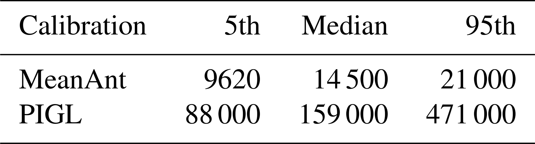
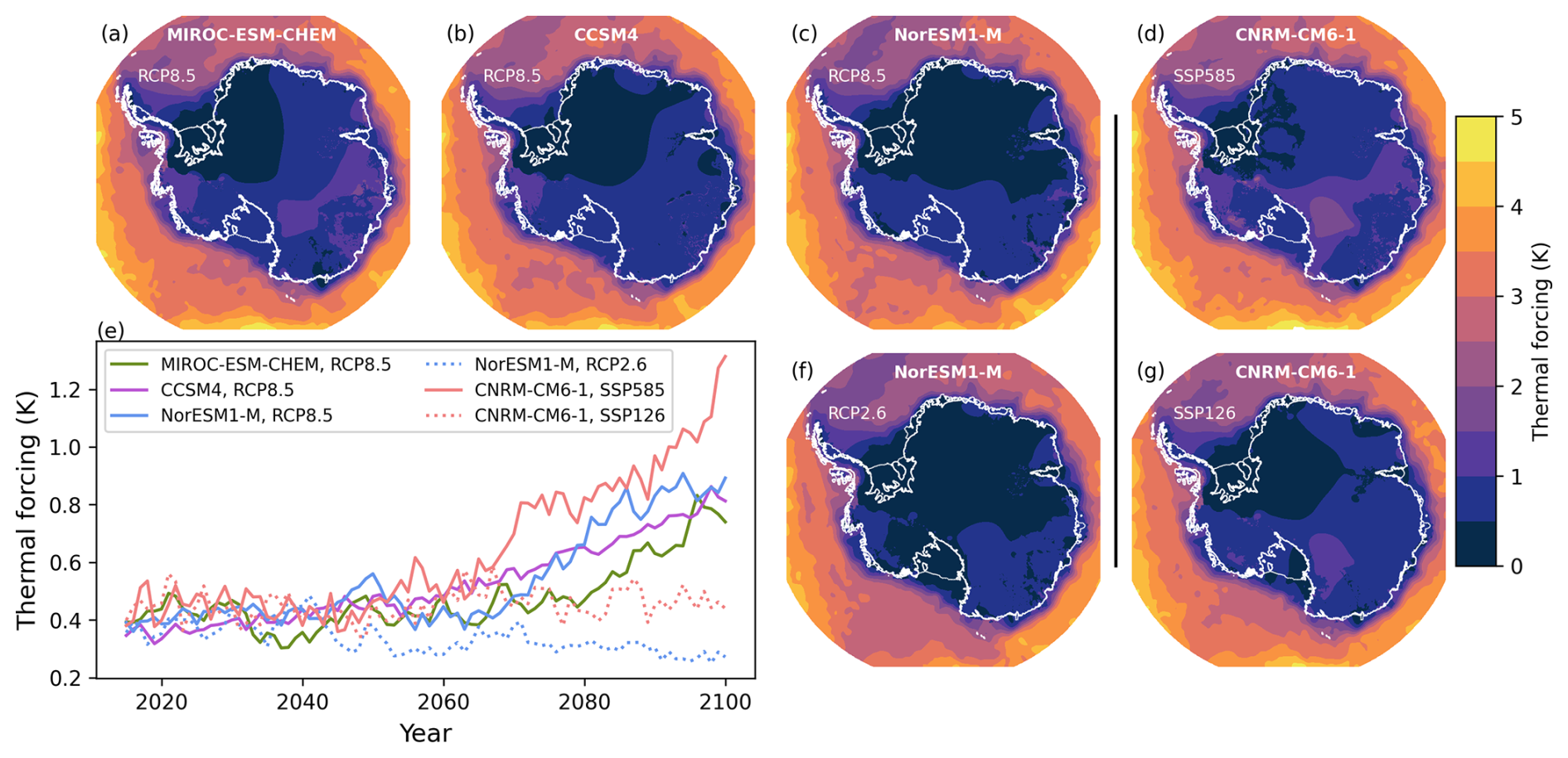
Figure 1 Thermal forcing averaged over the upper ocean (0–500 m) from 2015 to 2100 for MIROC-ESM under RCP8.5 (a), CCSM4 under RCP8.5 (b), NorESM1-M under RCP8.5 (c), NorESM1-M under RCP2.6 (f), CNRM-CM6-1 under SSP5-8.5 (d), and CNRM-CM6-1 under SSP1-2.6 (g). Panel (e) shows Antarctic mean annual upper-ocean (0–500 m) thermal forcing from 2015 to 2100. The vertical black line separates CMIP5 models (under RCP scenarios) from the CMIP6 model (SSP scenarios).

For the ice–atmosphere interface, surface mass balance anomalies were provided directly from GCMs relative to a January 1995 to December 2014 reference period (Nowicki et al., 2016). The anomalies were added to a baseline surface mass balance from Arthern et al. (2006) following previous BISICLES studies (Cornford et al., 2016) and BISICLES initMIP experiments (Seroussi et al., 2019). This approach does not account for the evolving topography of Antarctica over the simulation period. Average surface mass balance anomalies for 2015 to 2100 are shown in Fig. 2.

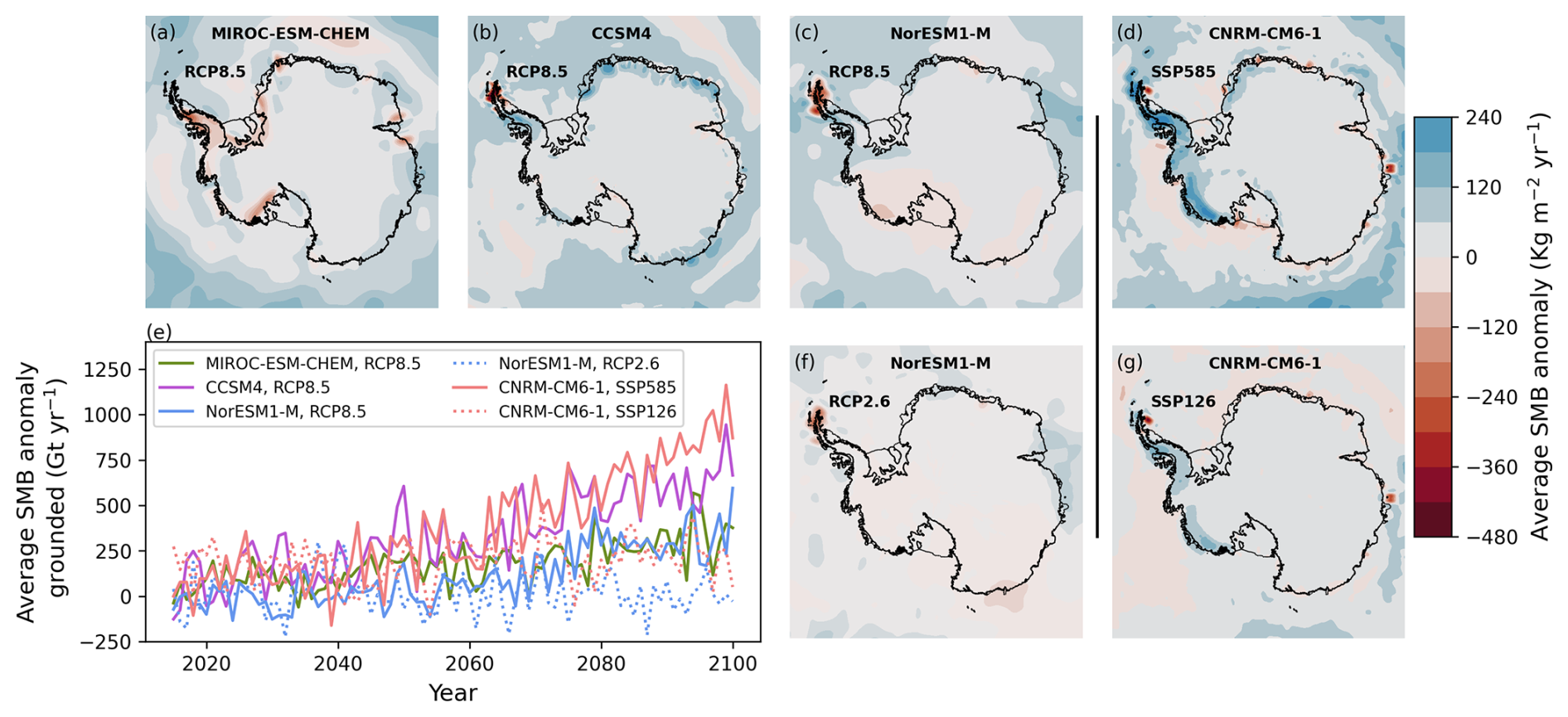
Figure 2 Surface mass balance anomaly (relative to 1995–2014) averaged from 2015 to 2100 for MIROC-ESM under RCP8.5 (a), CCSM4 under RCP8.5 (b), NorESM1-M under RCP8.5 (c), NorESM1-M under RCP2.6 (f), CNRM-CM6-1 under SSP5-8.5 (d), and CNRM-CM6-1 under SSP1-2.6 (g). Panel (e) shows the Antarctic mean annual surface mass balance anomaly from 2015 to 2100. The vertical black line separates CMIP5 models (under RCP scenarios) from the CMIP6 model (SSP scenarios).

Surface meltwater can enhance propagation of crevasses in ice shelves, driving weakening and eventual collapse (Scambos et al., 2009). However, inclusion of melt-driven hydrofracture, subsequent shelf collapse, and unstable grounded ice retreat is a relatively recent innovation in ice sheet models (Pollard et al., 2015). Questions remain around collapse mechanisms, the resulting rate of retreat (Crawford et al., 2021), and the importance of these mechanisms for past (Edwards et al., 2019) and future 21st century (Morlighem et al., 2024) Antarctic stability. Hydrofracture-driven shelf collapse is not directly implemented in those models participating in ISMIP6. ISMIP6 therefore provide time-dependent masks of ice shelf collapse to represent surface-melt-enhanced ice shelf disintegration. The masks are derived from atmospheric forcing projections: if surface-air-temperature-driven melt of 725 mm yr⁻¹ water equivalent persists for 10 years, the ice shelf is removed (Trusel et al., 2015; Seroussi et al., 2020).

We explore the impact of shelf collapse with two pairs of experiments (Table 2). Both sets of collapse on simulations use the same shelf collapse mask, i.e. derived from the same climate model projections (CCSM4). In these experiments, shelf collapse progresses southward during the experiment from the Antarctic Peninsula towards the South Pole. In these experiments, ∼ 30 % of the original Bedmap2 ice shelf area is removed by 2100.

2.3 Control simulation

The ISMIP6 protocol subtracts a control simulation from each projection simulation to remove model drift (Nowicki et al., 2016) and more easily compare results from different ice flow models with varying drifts. Our control simulation uses the Arthern et al. (2006) surface mass balance forcing. Basal melting is applied such that localised thickening as a result of ice advection or surface mass balance is removed. Basal melt driven by ocean thermal forcing is not applied, and accumulation onto the lower surface is not permitted (see BISICLES_B in Seroussi et al., 2019). Ice shelves can thin locally due to advection of ice out of grid cells. Treating the background melt field in this way maintains constant shelf thickness in most areas but ensures that the large melt rates immediately downstream of the grounding line are maintained should the grounding line advance or retreat. Control experiment boundary conditions are detailed further in Supplement Sect. 1.4.

3 Results

3.1 Control simulation results

From 2015 to 2100, the control simulation loses 19 220 Gt of mass above floatation, contributing 53 mm to sea level (Fig. 3c). The ice sheet area decreases by 6.9 × 10³ km², while the floating area increases by 64.6 × 10³ km². Average sea level contribution is 0.62 mm yr⁻¹ over this period, compared with an implied rate of 0.41 mm yr⁻¹ from 1992 to 2020 based on observations (Otosaka et al., 2023).

Thinning occurs over large regions of the Amundsen Sea sector, with some grounding line retreat at Thwaites Glacier (Fig. 3a). Major ice shelves (Ross, Filchner–Ronne, and Amery) also thin, as do their tributary ice streams. However, thinning of Lambert Glacier (Fig. 3b) is less pronounced than in some ice streams on the Siple Coast or those feeding the Filchner–Ronne Ice Shelf, consistent with a limited response of this catchment to ice shelf thinning in previous studies, e.g. Gong et al. (2014). In East Antarctica, ice streams at the margins around Totten Glacier and the Wilkes Basin (Fig. 3c) all undergo thinning in the control experiment.

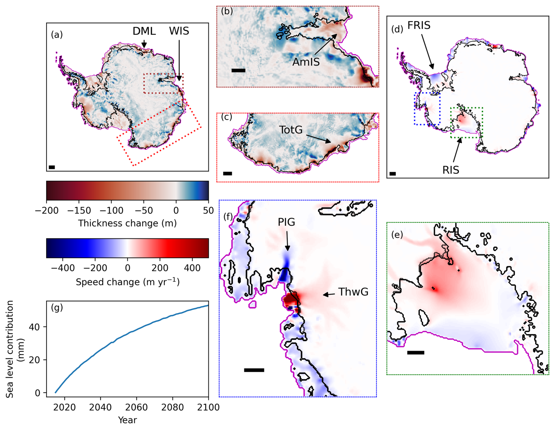
Figure 3 Control simulation (2015–2100). Panel (a) shows the thickness change between 2015 and 2100 in metres for the Antarctic Ice Sheet. Locations mentioned in the main text are indicated by arrows, i.e. Dronning Maud Land (DML) and the West Ice Shelf (WIS). Panel (b) focuses in on thickness change in the Amery Ice Shelf (AmIS, indicated by an arrow) and Lambert Glacier and corresponds to the dashed brown box in (a). Panel (c) shows the thickness change for East Antarctica in the region of the Totten Glacier (TotG, approximate outlet location indicated by an arrow) and the Wilkes basin and corresponds to the dashed red box in (a). Panel (d) shows the change in ice speed between 2015 and 2100 (in m yr⁻¹). The major ice shelves (Filchner–Ronne Ice Shelf: FRIS; Ross Ice Shelf: RIS) are indicated by arrows. Panel (e) highlights the speed change for the Ross Ice Shelf and Siple Coast glaciers and corresponds to the dashed green box in (d). Panel (f) highlights the speed change for the Amundsen Sea embayment glaciers and corresponds to the dashed blue box in (d). The locations of Pine Island (PIG) and Thwaites (ThwG) glaciers mentioned in the main text are indicated by arrows. Panel (g) shows the sea level contribution for the control simulation. The black scale bars in (a)–(f) correspond to 100 km. The solid black contour in (a)–(f) shows the 2015 grounding line position, while the dotted black contour shows the 2100 grounding line position. The purple contour in panels (a)–(f) shows the 2015 shelf edge position.

The most pronounced ice stream speed-up in the control simulation occurs for the Thwaites Glacier and its ice shelf (Fig. 3f) in response to grounding line retreat. By contrast, Pine Island Glacier maintains its grounding line position and slows down between 2015 and 2100 in the control run (Fig. 3f). Pine Island slow-down corresponds with shoaling of ice surface gradients over this period (not shown). Along the Siple Coast, Whillans Ice Stream (Ice Stream B) accelerates between 2015 and 2100, with grounding lines in this sector undergoing modest retreat (Fig. 3e). Overall, outer edges of major ice shelves slow down over the simulation period, with the exception of some ice shelves on Dronning Maud Land and the West Ice shelf (Fig. 3d). In these latter sectors, localised grounding line retreat is associated with speeding up of ice across the grounding line and out to the shelf edge.

3.2 Projected sea level contribution

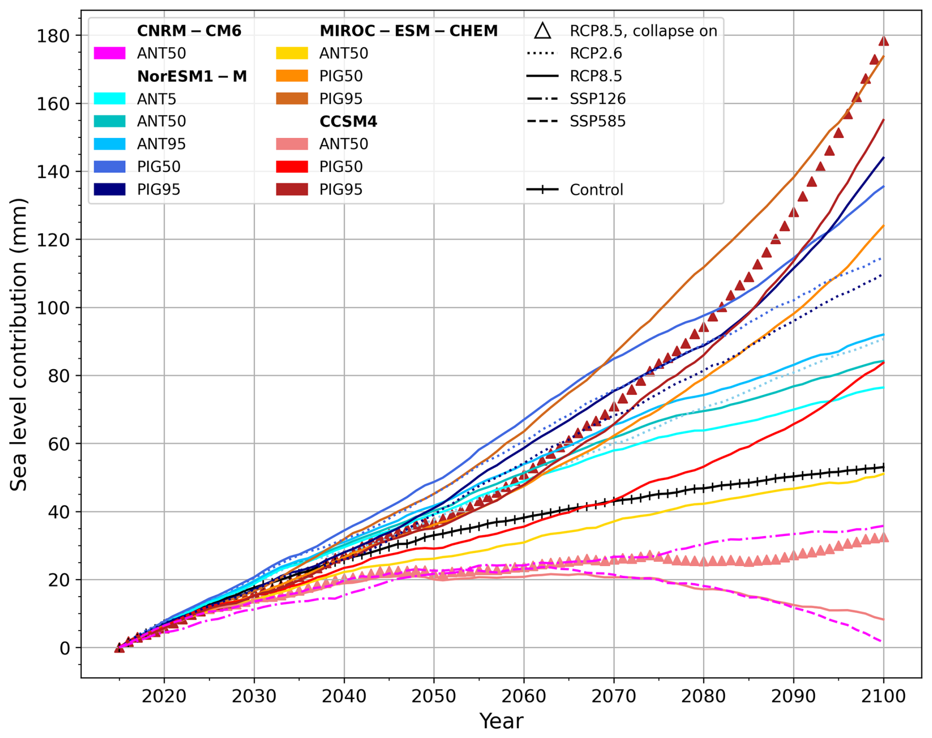
Projected sea level contribution from 2015–2100 varies between 2 and 178 mm across the 18 experiments (Table 2; Fig. 4). Five have a smaller sea level contribution than the control. All of these use the lower basal melt (MeanAnt) parameterisation and are forced by two of the four GCMs (CCSM4 from CMIP5 and CNRM-CM6-1 from CMIP6), while four of the five are under very high-emission scenarios (RCP8.5 or SSP5-8.5).

Table 2 Experiment list with projected sea level contribution minus the control simulation from 2015 to 2100 and sea level contribution (SLC) without the control subtracted (as quoted in Sects. 3–4).

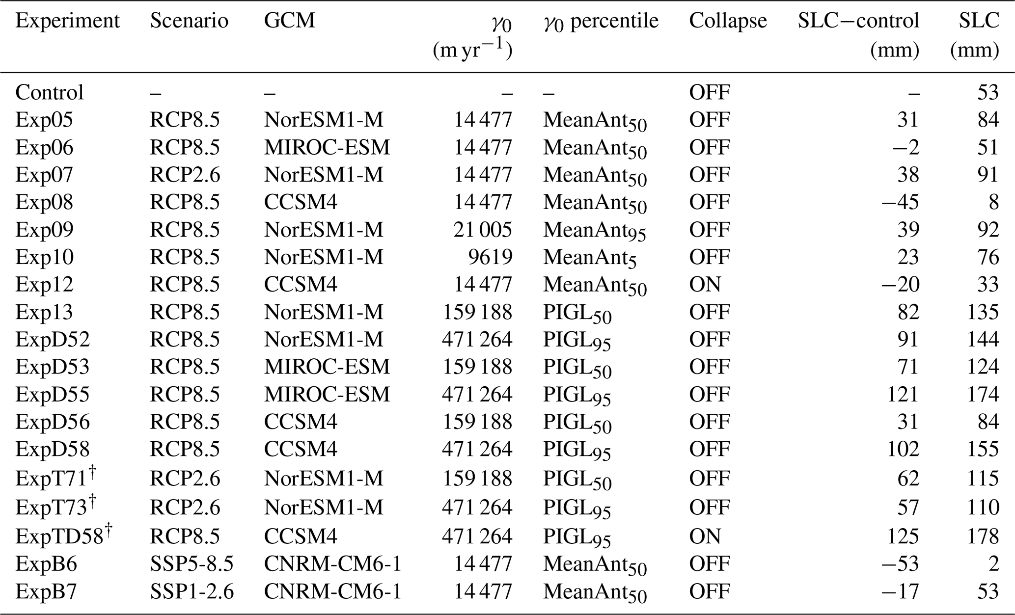
^† New experiments that were not part of the ISMIP6 protocol.

Figure 4 Sea level contribution (mm) for all experiments from 2015 to 2100.

3.3 Projected changes in ice area

Grounded ice sheet area changes are shown in Fig. 5 and grouped by GCM forcing. All simulations lose grounded area by 2100, with the exception of those forced by NorESM1-M under low emissions (RCP2.6) using the high basal melt parameterisation (PIGL₉₅), although under PIGL₅₀ and PIGL₉₅ the decrease is not monotonic. Perhaps counter-intuitively, initial grounded area increases with greater basal melt sensitivity to thermal forcing (i.e. higher values of γ₀, as shown by darker colours in Fig. 5). The differences in experiments between MeanAnt percentiles are small because the γ₀ values are relatively similar (Table 1). However, high basal melt sensitivity (PIGL) experiments decrease in grounded area much more quickly, and they generally lead to smaller final values than the MeanAnt experiments despite their larger areas in 2015.

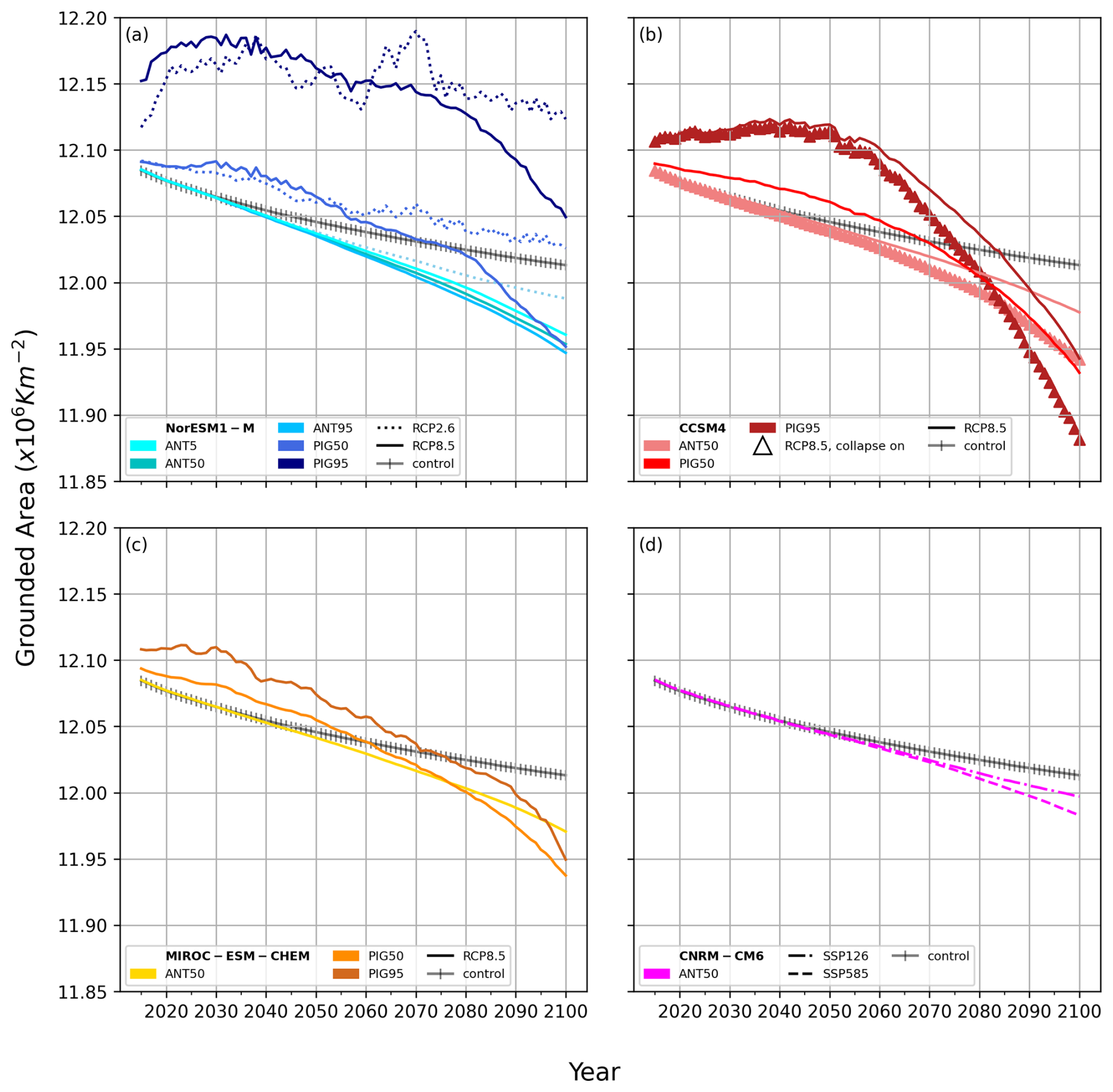
Figure 5 Grounded ice sheet area for all simulations from 2015 to 2100. Darker colours indicate higher γ₀ values. The panels show the grounded area for NorESM1-M (a), CCSM4 (b), MIROC-ESM-CHEM (c), and CNRM-CM6 (d) experiments from 2015 to 2100. Discrepancies in the initial area here and in Fig. 6 are due to our simulations beginning in 2010, whereas we show the 2015 to 2100 results for consistency with ISMIP6.

Figure 6 Floating ice sheet area for all simulations from 2015 to 2100. Darker colours indicate higher γ₀ values. The panels show the grounded area for NorESM1-M (a), CCSM4 (b), MIROC-ESM-CHEM (c), and CNRM-CM6 (d) experiments from 2015 to 2100.

In contrast, the floating ice area is larger at 2100 compared with 2015 for all experiments, with the exception of those with ice shelf collapse (CCSM4, shown as triangles in Fig. 6) and the experiment forced with NorESM1-M under RCP2.6 using the high basal melt parameterisation (PIGL₉₅). This response, i.e. reduced grounded ice sheet area and increased floating area, is consistent with grounding line retreat and loss of volume above floatation, with fixed-front calving maintaining the shelf edge position, meaning that the floating area increases as ice becomes ungrounded. In “collapse off” experiments, automatic calving of shelf ice thinner than 10 m can result in loss of up to ∼ 4 % of initial floating area. For collapse on experiments, loss of floating area from shelf collapse is partially offset by increases from grounding line retreat. Haseloff and Sergienko (2018) show that ice shelf buttressing can stabilise grounding lines, including on reverse-sloping beds. Our fixed-front calving approach may therefore under-predict sea level contribution, particularly for buttressed ice streams such as Pine Island. Moreover, lack of calving may maintain buttressing and could contribute to ice shelf slow-down in the control.

3.4 Regional sea level contributions

To explore the distinct responses of the West Antarctic Ice Sheet (WAIS), East Antarctic Ice Sheet (EAIS), and the Antarctic Peninsula (AP) to perturbed boundary conditions and basal melt sensitivity, we separate sea level equivalent mass change for these three regions (Fig. 7, Supplement Table 1). For the WAIS, sea level contribution ranges from 15 to 139 mm (Fig. 7a). Two simulations have a smaller WAIS sea level contribution than the control. Projected sea level contribution for the EAIS ranges from 65 to −32 mm (Fig. 7b). Four simulations gain mass in the EAIS, while six have a smaller sea level contribution than the control. Projections of Antarctic Peninsula sea level contribution range from −3 to 13 mm (Fig. 7b), and 10 experiments have a smaller sea level contribution than the control.

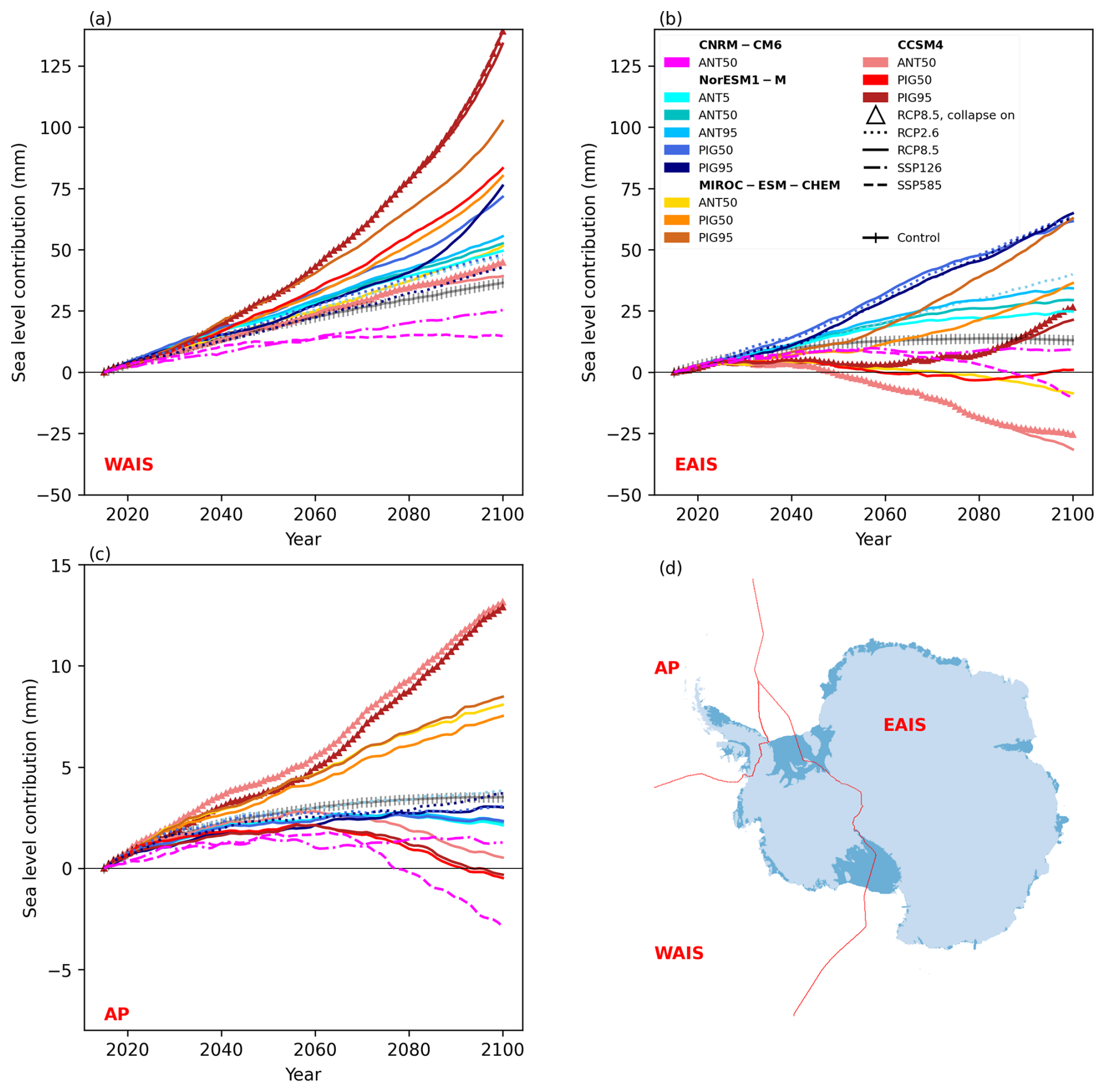
Figure 7 Sea level contribution (loss of volume above floatation) (mm) for the West Antarctic Ice Sheet (WAIS) (a), East Antarctic Ice Sheet (EAIS) (b), and Antarctic Peninsula (AP) (c) from 2015 to 2100. The inset shows the mask boundaries used to calculate regional change in volume above floatation. We note that the AP (c) has a truncated y axis compared with the WAIS (a) and EAIS (b) to aid legibility.

To further partition SLE ice sheet mass change, results are presented for the 16 drainage basins defined by Jourdain et al. (2020) (Fig. 8). The Amundsen Sea embayment (ASE) sector (10, Fig. 8j) has the largest sea level contribution of all 16 basins in 10 experiments, ranging from 21 to 62 mm (Supplement Table 1). This reflects patterns of thinning in the region across all experiments (Supplement Fig. S5). It exceeds the control sea level contribution in all but two experiments. With a sea level contribution of 26 mm, the ASE undergoes the largest mass loss in the control experiment. The Totten Glacier sector (5, Fig. 8e) has the largest sea level contribution of any sector in eight experiments, and sea level contribution ranges from 9 to 52 mm, with grounded ice thinning here in all experiments (Supplement Fig. S5). It exceeds the control sea level contribution in all but one experiment.

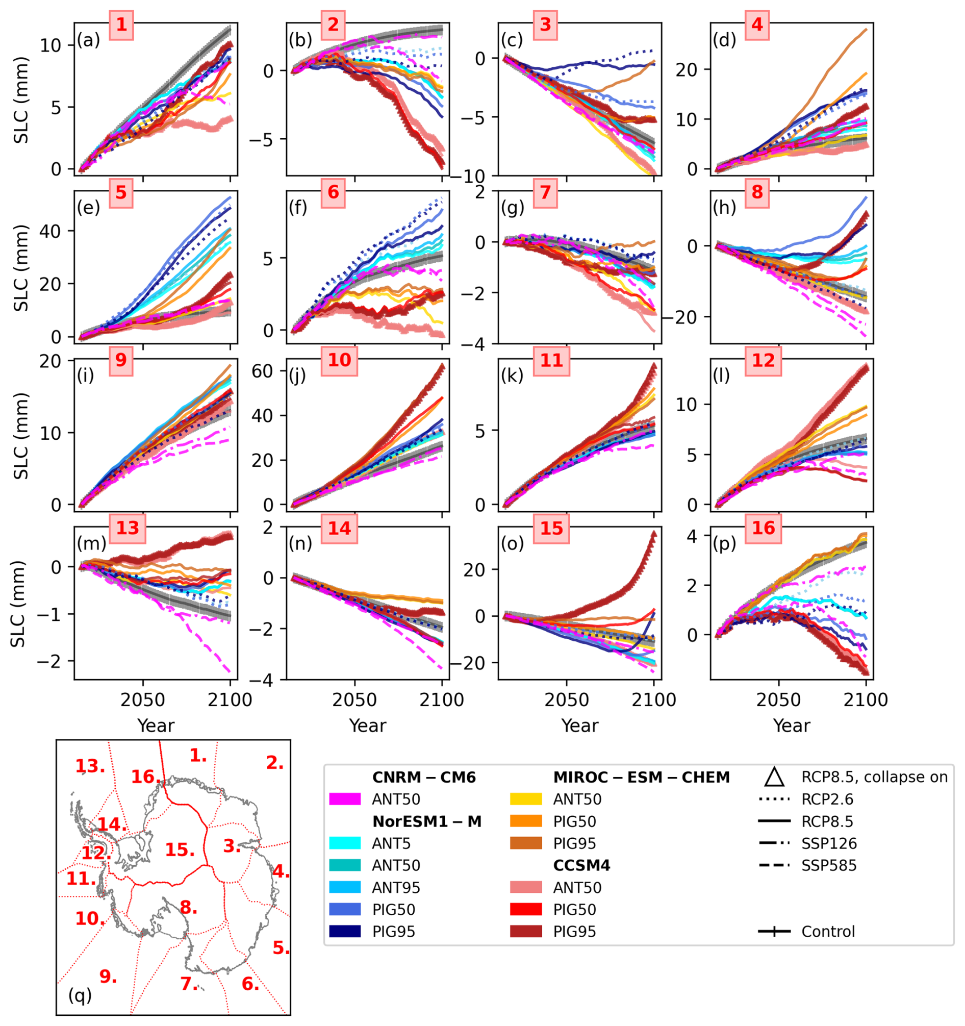
Figure 8 Sea level contribution by sector for all simulations. Basins are numbered are as follows: (1) Dronning Maud Land, (2) Enderby Land, (3) Lambert Glacier catchment, (4) Wilhelm II land, (5) Totten Glacier sector, (6) George V Land, (7) Oates Land, (8) Ross Ice Shelf, (9) Getz Ice Shelf sector, (10) Amundsen Sea embayment sector, (11) Abbott Ice Shelf sector, (12) George VI Ice Shelf sector, (13) Larsen Ice Shelf sector, (14) Palmer Land, (15) Filchner–Ronne Ice Shelf sector, and (16) Brunt Ice Shelf sector. Note the different scales on the y axes.

In the Filchner–Ronne Ice Shelf sector (16, Fig. 8o), 14 simulations increase their VAF relative to 2015 up to −24 mm sea level contribution, with −11 mm sea level contribution in the control. The Filchner–Ronne drainage basin has a large area over which to accumulate mass, which offsets mass loss due to ocean melting. However, the Filchner–Ronne Ice Shelf sector loses mass equivalent to a 35 mm sea level contribution under high basal melt sensitivity and CCSM RCP8.5, giving it the largest projected range of any sector (−24 to 35 mm sea level contribution, SLC). The projected range in this sector illustrates the competing processes of increased accumulation under warming (Payne et al., 2021) and increased mass loss due to basal melting. When sensitivity to ocean melt is low, increased accumulation dominates ocean melt-driven mass loss. Conversely, under higher ocean melt sensitivity, ocean melt-driven mass loss counteracts the warming-driven negative surface mass balance (SMB) feedback. The importance of this compensation effect in determining the Filchner–Ronne Ice Shelf sector sea level contribution has been demonstrated previously, e.g. in Cornford et al. (2015) and Wright et al. (2014). Under the highest basal melt sensitivity, the loss of VAF in the Filchner–Ronne Ice Shelf sector is 55 mm greater than under equivalent lower-ocean-sensitivity scenarios with the same forcing (Supplement Table 1).

The other sector with a major ice shelf, the Ross Sea sector (8, Fig. 8h), gains mass in all but four experiments, with a sea level contribution range of −26 to 14 mm, with the highest contribution under NorESM1-M RCP8.5 and the second-highest basal melt sensitivity (Supplement Table 1). For the two highest sea level contribution experiments for the Filchner–Ronne Ice Shelf sector (CCSM4, RCP8.5, highest basal melt sensitivities), the Ross Sea sector contributes 9 mm to sea level. Mass gain for the major ice shelf sectors, despite ice shelf thinning and reduced buttressing (Supplement Fig. S5) in most experiments, reflects the large contribution to mass gain from accumulation over their grounded area.

For ISMIP6, participating models subtract the control simulation to account for model drift. However, the large sectoral contribution in our experiment suggests that this removes the sea level signal from the ASE's long-timescale response to retreat initiated before 2015. It is not clear that marine ice sheet instability (MISI) has been initiated in the ASE, with the IPCC AR6 stating that observed flow regimes in the ASE are compatible with but not incontrovertible evidence of MISI (Fox-Kemper et al., 2021). In contrast, both the Ross Sea and Filchner–Ronne Ice Shelf sectors steadily increase in VAF throughout the control simulation, which is broadly consistent with 1979–2019 VAF trend in these regions (Rignot et al., 2019).

3.5 Dependence on GCM forcing

GCM dependence is driven by patterns of surface mass balance over the ice sheet (Fig. 9c, d, f) and patterns of ocean forcing, which is the main driver of ice shelf thinning and increased grounding line flux (Fig. 9a, b, e).

To explore this, we compare simulations using different GCM forcings but with the same ice shelf basal melt sensitivity and emission scenario. Under the MeanAnt₅₀ tuning and RCP8.5, the NorESM1-M-forced simulation contributes 84 mm to sea level, MIROC-ESM contributes 51 mm to sea level, and CCSM4 has a sea level contribution of 8 mm. Of these three GCMs under RCP8.5, CCSM4 has the highest SMB over the WAIS and EAIS, followed by MIROC-ESM and NorESM1-M (Fig. 9c and d). Moreover, for MIROC-ESM and CCSM4, the EAIS drives sea level fall, while the region loses mass under NorESM1-M (Fig. 7, as shown with solid pink (CCSM4), yellow (MIROC-ESM), and turquoise (NorESM1-M) lines). This reflects the smaller response in the NorESM1-M atmosphere to RCP8.5 warming compared with other CMIP5 models (Barthel et al., 2020), which limits the extent to which warming-driven increases in surface mass balance compensate for ocean-driven losses.

When higher basal melt sensitivity (PIGL₅₀) is used under the same emission scenario, NorESM1-M again has the largest sea level contribution at 135 mm. The MIROC-ESM-forced simulation contributes 124 mm to sea level, followed by CCSM4 with a sea level contribution of 84 mm. Under the highest basal melt sensitivity (PIGL₉₅), MIROC-ESM drives the largest sea level contribution at 174 mm, followed by CCSM4 at 155 mm. NorESM1-M has the smallest PIGL₉₅ sea level contribution at 144 mm (Fig. 7). With increased γ₀, GCM dependence becomes more dependent on ocean forcing, as surface mass balance forcing is the same for experiments with the same GCM scenario forcing. Increased sea level contribution for MIROC-ESM is partly driven by increases in EAIS mass loss (Fig. 9b), e.g. sectors 4 (Queen Mary Land) and 5 (Totten Glacier sector) (Fig. 8d, e, respectively), where thermal forcing is high (Fig. 1). Similarly, NorESM1-M undergoes large mass loss in the EAIS where SMB is low, while grounding line flux increases under high γ₀ (Fig. 9b). On the WAIS, ocean thermal forcing drives a large grounding line flux under CCSM4 (Fig. 9a), particularly under high γ₀.

We also ran two simulations forced with a newer climate model (CMIP6) under newer emission scenarios (SSPs). Comparing the CNRM-CM6-1 SSP5-8.5 with the other high-emission-scenario CMIP5-forced experiments with MeanAnt₅₀, we see a lower sea level contribution at 2 mm. This is the lowest sea level contribution of any experiment. High SMB in all regions (Fig. 9c, d, f) and low thermal forcing (Fig. 1) and grounding line flux (Fig. 9a, b, c) values compared with other experiments result in less mass loss than other comparable experiments or the control (Table 2).

3.6 Dependence on emission scenario

The higher-warming simulations (RCP8.5 for CMIP5 models and SSP5-8.5 for CMIP6) generally have higher SMB over the continent (Fig. 9) than low-emission-scenario experiments, consistent with larger precipitation flux under warming (Payne et al., 2021; Palerme et al., 2017; Frieler et al., 2015). The scenario dependence was then modulated by the value used for basal melt sensitivity.

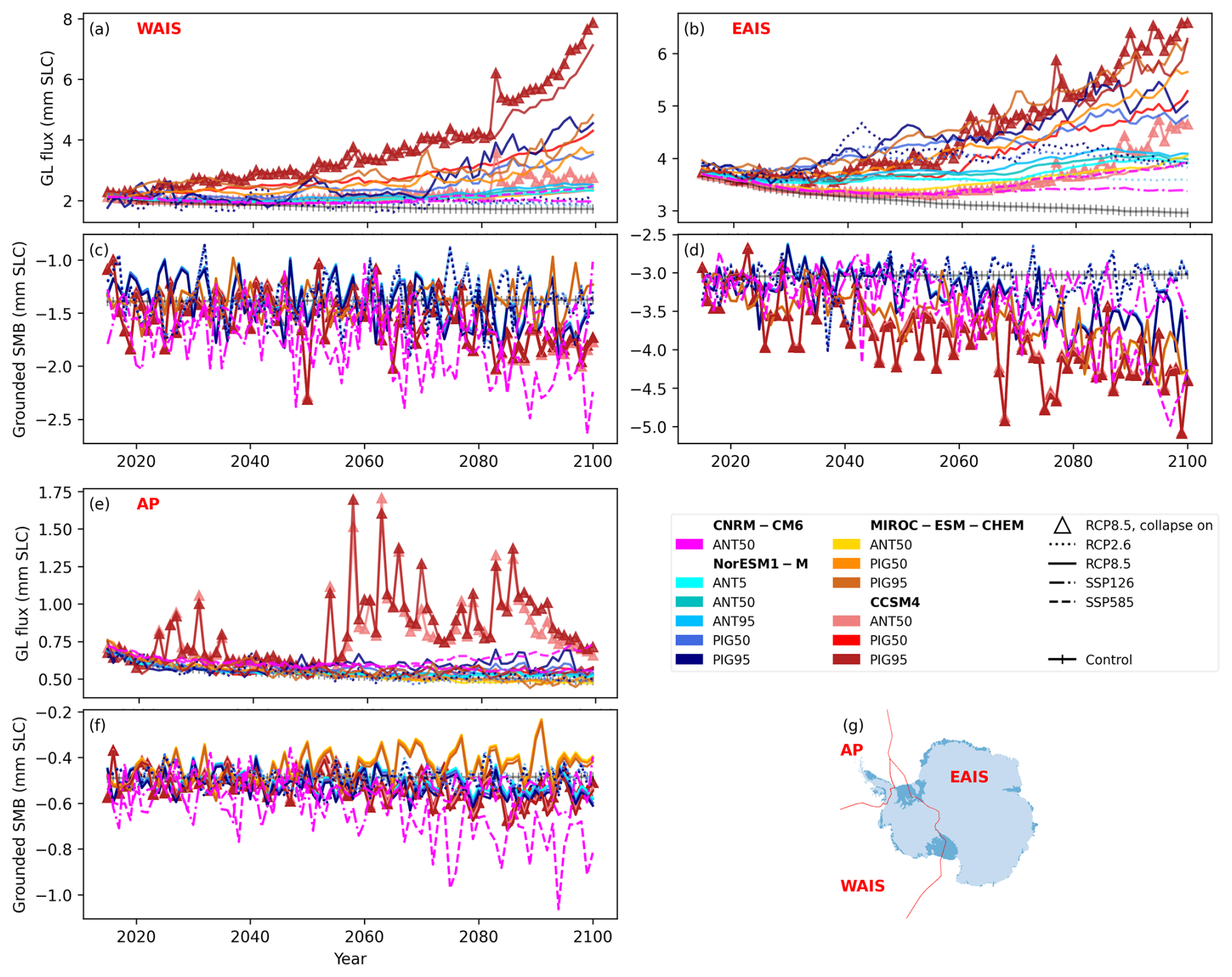
Figure 9 Total annual grounding line flux (mm SLC, positive values for mass loss) for the West Antarctic Ice Sheet (WAIS) (a), the East Antarctic Ice Sheet (EAIS) (b), and the Antarctic Peninsula (AP) (e). Annual surface mass balance integrated over the grounded area of each region (mm SLC, where negative values indicate ice sheet mass gain) for the WAIS (c), EAIS (d), and AP (f). Region boundaries are also shown (g). Note that scale of the y axis differs between panels.

Scenario dependence was assessed for the two GCMs used to make projections under the low-emission scenarios (RCP2.6/SSP1-2.6), NorESM1-M from CMIP5 and CNRM-CM6-1 for CMIP6, and it was calibrated to mean Antarctic melt rates. For the NorESM1-M simulations, the low-emission scenario leads to greater sea level contribution by 2100, which is counter to the intention of mitigating climate impacts (91 mm under RCP2.6 compared with 84 mm under RCP8.5). This varies regionally: WAIS sea level contribution, for example, is smaller under RCP2.6 than RCP8.5 (47 mm vs. 53 mm), as basal melting under RCP8.5 is greater (Fig. 9a), while SMB is lower under RCP2.6 (Fig. 9b). These factors together drive the higher mass loss in WAIS under RCP8.5 compared with RCP2.6 – consistent with other ISMIP6 ice sheet models forced by NorESM1-M, where mass loss is greater under RCP8.5 than RCP2.6 (Fig. 4a in Edwards et al., 2021). For the EAIS and the majority of the AP, the SMB scenario dependence is reversed: SMB is higher under RCP8.5 compared with RCP2.6. This drives a smaller net sea level contribution in the EAIS under RCP8.5 (29 mm vs. 40 mm under RCP2.6) and in the AP compared with RCP2.6 (4 mm vs. 2 mm under RCP8.5), which is consistent with most other ISMIP6 models (Fig. 4c, d in Edwards et al., 2021).

Simulations forced by the CMIP6 model CNRM-CM6-1 project low sea level contribution under both emission scenarios: 2 mm under SSP5-8.5 and 53 mm under SSP1-2.6. The WAIS, EAIS, and AP all have less mass loss under SSP5-8.5 compared with SSP1-2.6. Unlike NorESM1-M, CNRM-CM6-1 consistently has higher SMB under the higher-emission scenario across the majority of the ice sheet (Fig. 9a, b, e). Basal melt is higher under the higher-emission scenario for CNRM-CM6-1 (Fig. 9c, d, f), albeit not by enough to counteract the SMB increases, meaning that sea level contribution is smaller for all sectors (WAIS: 25 mm vs. 15 mm; EAIS: 9 mm vs. −10 mm; AP: 1 mm vs. −3 mm). This is consistent with other ISMIP6 projections forced with this climate model, where accumulation under higher emissions exceeds ocean melt-driven mass loss (Fig. 4 in Edwards et al., 2021).

Two additional simulations beyond the ISMIP6 protocol (T71 and T73) were run to provide insight into the modulation of scenario dependence by basal melt sensitivity. These apply NorESM1-M thermal forcing under RCP2.6 with PIGL₅₀ and PIGL₉₅ basal melt sensitivity parameters. For the AP and EAIS, sea level contribution is comparable under both scenarios and γ₀ values (Supplement Table 1), indicating limited scenario dependence under PIGL₅₀ and PIGL₉₅ for NorESM1-M. For the WAIS, sea level contribution increases by 33 and 34 mm under PIGL₅₀ and PIGL₉₅, respectively (Supplement Table 1). Under the Ross Ice Shelf, thermal forcing increases more under RCP8.5 compared with RCP2.6 than under the Filchner–Ronne Ice Shelf. For PIGL₅₀, RCP8.5 increases sea level contribution by 28 mm in the Ross Sea sector from −15 mm sea level contribution under RCP2.6 (sector 8, Fig. 8h, Supplement Table 1). Conversely, the Filchner–Ronne Ice Shelf sector gains mass under both RCP8.5 (−15 mm SLC) and RCP 2.6 (−9 mm SLC) under PIGL₅₀. This demonstrates greater scenario dependence in the Ross Sea sector compared with the Filchner–Ronne Ice Shelf sector. These experiments informed the assessment of potential interactions between scenario and basal melt sensitivity (see Sect. 4.3).

For both scenario dependence and GCM dependence, climate model sensitivity plays a significant role. CNRM-CM6-1 has an equilibrium climate sensitivity (ECS) of 4.8 °C (Meehl et al., 2020) similar to MIROC-ESM-CHEM (ECS = 4.7 °C), which is the highest ECS CMIP5 model sampled in ISMIP6 and discussed in Payne et al. (2021). However, CNRM-CM6-1 ECS is higher than the remaining CMIP5 models, with CCSM4 and NorESM1-M both having an ECS of 2.9 °C (Flato et al., 2013). This drove large positive surface mass balance and accumulation in CNRM-CM6-1, compared with the simulation under the low-emission scenario (Fig. 9). This offset dynamical losses from ocean melt-driven retreat.

3.7 Dependence on ice shelf collapse

Two pairs of simulations explore the impact of shelf collapse on sea level contribution. All are forced with the CCSM4 climate model under RCP8.5. The first pair have ice shelf collapse on and off, with the MeanAnt₅₀ basal melt parameter value (experiment 12 and 8, respectively). The second pair is the same but with the PIGL₉₅ parameter value (experiment TD58 and D58) to explore the interactions between the basal melt parameter and shelf collapse. Experiment TD58 was beyond the ISMIP6 protocol and was performed to inform the synthesis by Edwards et al. (2021)

Including shelf collapse increases Antarctic sea level contribution by around 25 mm relative to “no collapse” in both pairs of experiments (by region, the increase is 13 mm for the AP, 5–6 mm for the EAIS, and 5–6 mm for the WAIS). However, the no collapse baseline is very different in the two basal melt parameterisations (8 mm sea level contribution under MeanAnt₅₀ compared with 155 mm under PIGL₉₅). These two sets of projections informed the assessment of interactions between ice shelf collapse and basal melt sensitivity (see Sect. 4.3).

3.8 Dependence on basal melt sensitivity

To understand the dependence of the projections on the basal melt parameter, experiments with the same GCM forcing and different γ₀ can be compared. Here all simulations have ice shelf collapse off. The most comprehensively sampled combination of a GCM and scenario is NorESM1-M under RCP8.5, where simulations were carried out for five basal melt sensitivity values: MeanAnt₅, MeanAnt₅₀, MeanAnt₉₅, PIGL₅₀, and PIGL₉₅. Three of these values (MeanAnt₅₀, PIGL₅₀, and PIGL₉₅), which span most of the range, were also carried out for NorESM1-M under RCP2.6 and for MIROC-ESM and CCSM4 under RCP8.5.

The overall γ₀ dependence for the majority of GCMs is one of increased sea level contribution under higher γ₀, as discussed throughout the results, though the nature of this relationship varies by region and GCM (Fig. 10). The Antarctic Peninsula is fairly insensitive to increases in γ₀ (Fig. 10c). In comparison with other ISMIP6 models, BISICLES has intermediate sensitivity to γ₀ (see Fig. 6 in Edwards et al., 2021).

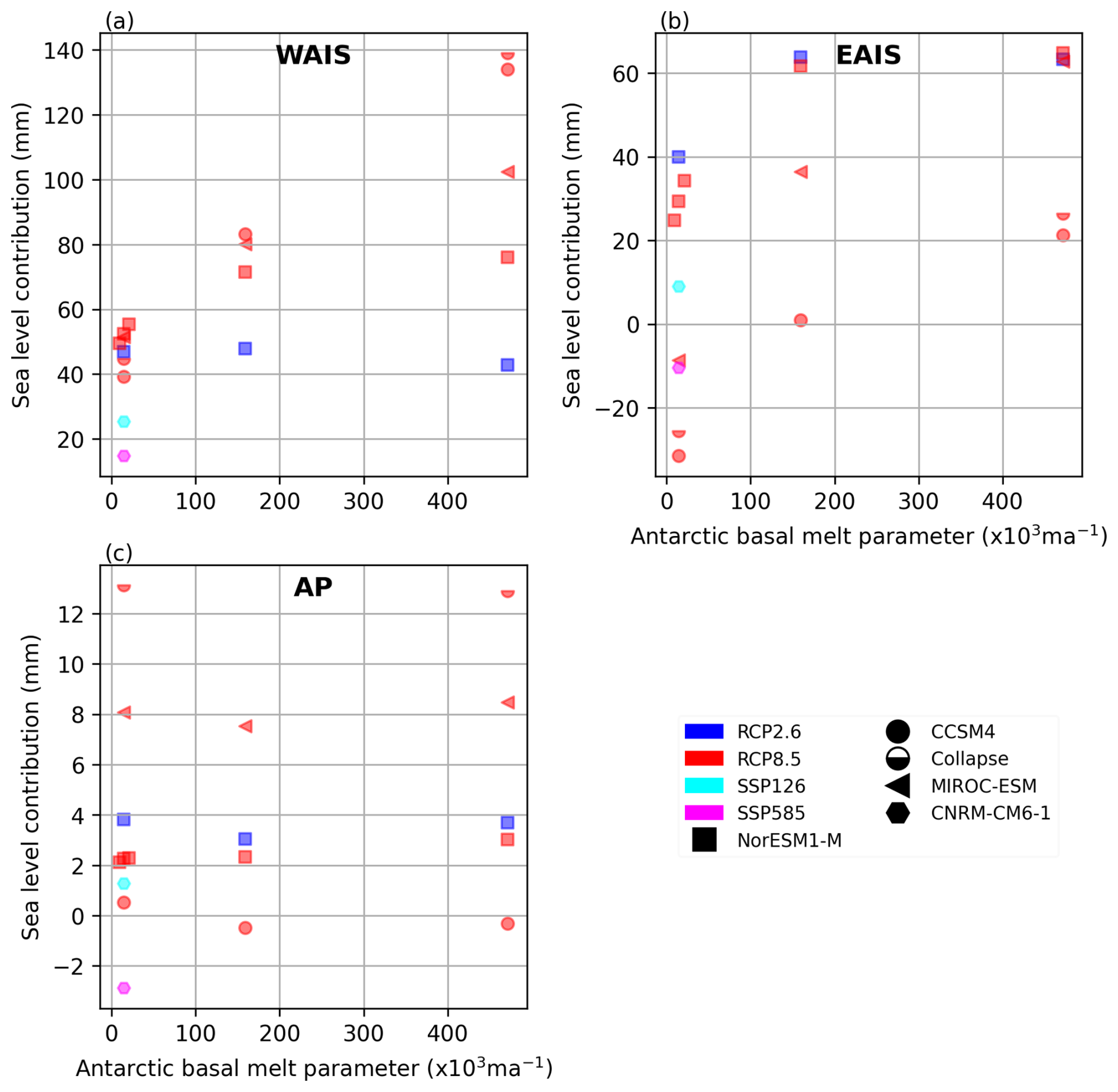
Figure 10 Sea level contribution from 2015 to 2100 for all simulations as a function of basal melt sensitivity (γ₀) for the West Antarctic Ice Sheet (WAIS) (a) East Antarctic Ice Sheet (EAIS) (b), and Antarctic Peninsula (AP) (c).

In the NorESM1-M experiments, increasing γ₀ from PIGL₅₀ to PIGL₉₅ leads to a more complex response in the WAIS and EAIS than the simple increase in sea level contribution seen for other GCMs (Fig. 10a and b). Under RCP2.6, the PIGL₉₅ simulation counter-intuitively undergoes a smaller loss of VAF than the PIGL₅₀ simulation (Fig. 4, dashed dark blue lines). While localised thickening occurs intermittently for all GCMs and scenarios under PIGL basal melt tuning (not shown), for NorESM1-M thickening is pervasive enough to alter the dependence of net mass loss on γ₀. As can be seen in Supplement Fig. 5g and h, the Ross Ice Shelf thickens in both simulations, with more thickening under PIGL₉₅. Under RCP8.5, the PIGL₉₅ simulation also projects a smaller contribution to sea level than PIGL₅₀ for most of the century until overtaking it in 2094 (Fig. 4, solid blue lines) for the whole ice sheet.

4 Discussion

4.1 Basal melt sensitivity

In terms of basal melt sensitivity, previous studies using ISMIP6 non-local basal melt parameterisation have also noted ice shelf thickening as a result of refreezing under high γ₀ values (Lowry et al., 2021; Lipscomb et al., 2021). Ice shelf refreezing under low thermal forcing is plausible and present in observations and model simulations of Antarctic ice shelf cavities (Naughten et al., 2018; Adusumilli et al., 2020; Reese et al., 2018; Stevens et al., 2020). However, Lipscomb et al. (2021) modify the second term in Eq. 1 to avoid what they suggest is spurious melting and refreezing where $\langle \mathrm{TF}{\rangle }_{\mathrm{draft}\in \mathrm{sector}}+\mathit{\delta }{T}_{\mathrm{sector}}$ is negative. An earlier study exploring Antarctic sensitivity to future climate and model parameters used an alternative basal melt approach that also avoids refreezing of ice shelves by design (Bulthuis et al., 2019).

Our BISICLES version uses the ISMIP6 non-local melt parameterisation without modification (Jourdain et al., 2020). However, thickening of ice shelves as a result of the basal melt parameterisation is not permitted in this BISICLES_B configuration. Thickening of ice shelves under the highest γ₀ values could therefore be a manifestation of tributary glaciers responding to strong ice shelf thinning, removal of buttressing, and advection of ice to grounding lines as ice streams speed up. Beyond 100-year timescales, initial thickening could therefore precede a larger long-term sea level response. Future work could explore whether melt sensitivity dependence for the highest γ₀ values reverts to that seen for lower values (higher γ₀, more mass loss) over longer timescales.

The Ross Sea sector provides an example of an ice shelf and grounding line dynamic under PIGL γ₀ tuning that runs counter to our expectation that higher γ₀ will increase shelf thinning and enhance grounding line retreat. For this and other sectors under NorESM1-M RCP2.6 and RCP8.5 (e.g. sector 4 (Totten Glacier) and sector 5 (George V Land)), sea level rise contribution under the highest basal melt sensitivity (PIGL₉₅) is lower than under the second-highest (PIGL₅₀) basal melt sensitivity (Fig. 8, solid blue lines). Figure 11a shows a transect through the grounding line at the terminus of Whillans and Mercer ice streams for PIGL₉₅ NorESM1-M RCP8.5 and PIGL₅₀ at three successive time slices (2015, 2050, and 2100). The basin-average thermal forcing for NorESM1-M RCP8.5 is also shown (Fig. 11c). In the Ross Sea sector, the grounding line under PIGL₉₅ is seaward of the equivalent PIGL₅₀ simulation grounding line for the duration of the simulation at the Whillans and Mercer ice streams grounding line (Fig. 11a). Ross Sea sector ice streams drain around 40 % of the West Antarctic Ice Sheet (Price et al., 2001), meaning that changes to ice stream configuration along the Siple Coast impact sea level contribution in the sector.

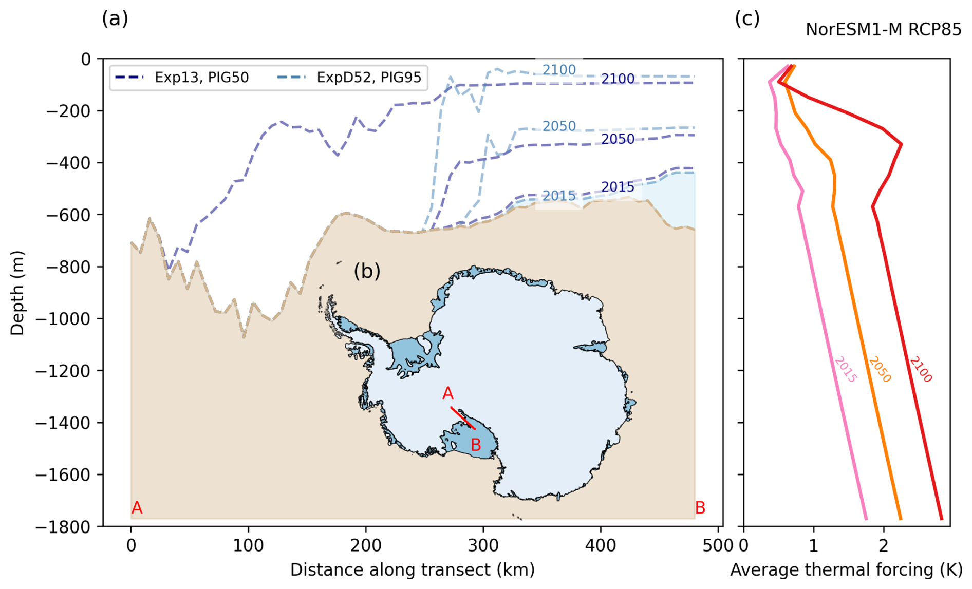
Figure 11 Panel (a) shows a transect through the Siple Coast for PIGL₅₀ (darker blue lines) and PIGL₉₅ (lighter blue lines) experiments under NorESM1-M RCP8.5. Dashed blue lines show ice sheet base for years indicated. Panel (b) shows average thermal forcing with depth at successive time steps. Panel (c) shows the transect location. The higher basal melt sensitivity (γ₀) run undergoes more thinning in the outer shelf shown in the transect, but the grounding line retreats further inland for the run with lower γ₀; however, the shelf remains thicker for the latter.

4.2 Comparison with other models

To explore differences between BISICLES and ISMIP6 contributions from other models, we first compare control simulations. As noted in Seroussi et al. (2020), models employing a data assimilation approach to initialisation have larger mass trends through the control simulation. Table B2 in Seroussi et al. (2020) presents total ice mass change, mass above floatation change, total area change, and floating area change for ISMIP6 control experiments. BISICLES undergoes a total mass change of −50 149 Gt and a mass above floatation change of −19 220 Gt between 2015 and 2100 in the control experiment. The magnitude of mass change for both total mass and mass above floatation is comparable to other models using a data assimilation type initialisation. Total area change in our control is −6.9 × 10³ km² – with any area loss associated with regions of the ice sheet where decreases in thickness to 10 m result in calving. Floating area increases by 6.46 × 10⁴ km², consistent with regional grounding line retreat described in Sect. 3.1. The average annual basal melt is 2139 Gt yr⁻¹ for our control simulation, while integrated surface mass balance is 2144 Gt yr⁻¹. This relatively low surface mass balance and high basal melting, combined with our data assimilation type initialisation, likely contributes to BISICLES having the fourth-highest mass loss in the control amongst ISMIP6 models (Seroussi et al., 2020, Table B2).

We next compare BISICLES projections with other ISMIP6 models and analyse regional contributions for experiments discussed in the main text and shown in Fig. 12. For the purpose of this comparison, we subtract the control from our simulations in line with the previous ISMIP6 results (Seroussi et al., 2020).

For the EAIS, BISICLES has the largest sea level contribution under mean Antarctic γ₀ tuning for NorESM1-M RCP8.5-forced simulations (Fig. 12a–d). With the largest EAIS contribution in these experiments being sourced from the Totten Glacier, this could suggest that BISICLES 1 km grid resolution at the Totten Glacier grounding line is resolving retreat not captured in lower-resolution models (4–20 km for fixed-resolution models; minimum 2 km for variable-resolution models) – though we note that Totten Glacier can retreat at lower resolution (<8 km) in BISICLES (Cornford et al., 2016). Previous studies have also highlighted that models using sub-grid interpolation schemes at the grounding line are more sensitive to forcing than conventional models (Tsai et al., 2015).

For the WAIS (Fig. 12e–k), BISICLES projections for the core experiments tend to be mid-range and similar to two models with structural similarities: CISM, which is the other L1L2 physics model (albeit run on a fixed 4 km grid), and UCIJPL ISSM, which also uses a variable mesh resolution. CISM additionally implements a sub-grid interpolation scheme to represent basal melt in partially floating cells (Lipscomb et al., 2021), which could account for its slightly larger sea level contribution under NorESM1-M RCP8.5 core experiments for the WAIS compared with BISICLES, which does not implement a sub-grid interpolation scheme for basal melting (Seroussi and Morlighem, 2018). Under increased basal melt sensitivity (γ₀), the CISM WAIS contribution is larger still. UCIJPL ISSM uses a variable mesh with a finest resolution of 3 km near the margins and has higher-order physics (Seroussi et al., 2020). Agreement between ISSM and BISICLES for core WAIS simulations could reflect high resolution in both models compared with other ISMIP6 models. We note that in the Marine Ice Sheet Model Intercomparison Project (MISMIP+), model physics had a less significant impact on simulated dynamics than the basal sliding law, which is based on Weertman sliding for both BISICLES and UCIJPL ISSM, at comparable resolutions (Cornford et al., 2020). While BISICLES and ISSM have Weertman sliding over much of the domain, BISICLES uses a Tsai et al. (2015) type sliding law with Coulomb sliding close to the grounding line. This difference could be a factor where higher sea level contributions are simulated in BISICLES. The millimetre-scale magnitude of this difference is comparable to that found in previous studies comparing Weertman-only and Tsai et al. (2015) type sliding laws (Nias et al., 2018; Barnes and Gudmundsson, 2022).

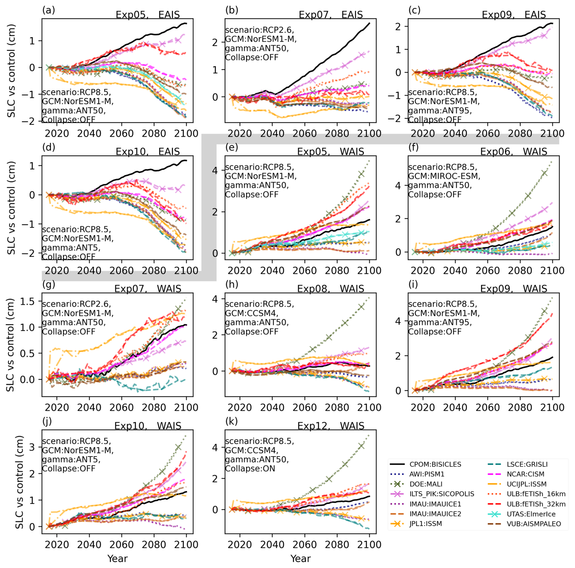
Figure 12 Comparison between BISICLES projections minus the control and other ISMIP6 models for experiments mentioned in this paper. The panels above the grey divider (a–d) are for the East Antarctic Ice Sheet (EAIS) contribution to core experiments. The panels below the grey divider (e–k) are for the West Antarctic Ice Sheet (WAIS) contribution to core experiments. Data are from Edwards et al. (2021).

4.3 Contributions to Edwards et al. (2021)

Simulations presented here were included in the synthesis of projections of global land ice contribution to 2100 sea level by Edwards et al. (2021), extending the ISMIP6 ensemble by an additional model compared with Seroussi et al. (2020) and Payne et al. (2021). Experiments beyond the main ISMIP6 protocol were also conducted to provide further exploration of sensitivities and interactions.

As outlined in Sect. 3.7, the increase in sea level contribution with collapse on is almost identical for both basal melt sensitivities sampled (MeanAnt₅₀ and PIGL₉₅), although the no collapse baseline is higher under PIGL₉₅. Along with results from the same experiments in ISSM, this is the basis for the conclusion in the “Ice shelf collapse versus basal melt” section of Edwards et al. (2021) that the contribution due to ice shelf collapse does not significantly increase with higher values of γ₀.

Sampling PIGL basal melt sensitivity under RCP2.6 (T71 and T73) and comparing it with RCP8.5 projections shows that the spread of projections is smaller under RCP2.6, as confirmed in complementary experiments with ISSM presented in the “Retreat and basal melt versus temperature” section of Edwards et al. (2021).

4.4 Limitations

Our work complements the ISMIP6 ensemble, providing high-resolution simulations of Antarctica with a physically comprehensive model and exploring uncertainties beyond the original ISMIP6 protocol. However, limitations remain, and these are outlined below.

For NorESM1-M RCP2.6 PIGL₉₅, the sea level contribution until 2100 is lower than that projected under PIGL₅₀. However, the trajectory of mass loss in Fig. 4 indicates that PIGL₉₅ could overtake PIGL₅₀ beyond 2100. Work is ongoing to extend these simulations to 2300 and will shed valuable light on mass loss under high basal melt sensitivity beyond 2100. More broadly, IPCC AR6 extrapolates mass trends from 2100, the end of the simulation period for the model inter-comparisons it draws on, to project sea level to 2150, which is a time horizon that is increasingly policy relevant for long-lived infrastructure (Fox-Kemper et al., 2021). With ice sheet model simulations beyond 2100, longer-term sea level projections should be informed by physics-based models without the need to assume mass trends.

Another informative extension on the work presented here would be to more comprehensively explore model uncertainties. We explored five of the six γ₀ values provided by ISMIP6, omitting an intermediate (PIGL₅) value from our experiments. Future simulations could include this γ₀ value. Moreover, while we were limited to the discrete γ₀ values provided by ISMIP6, as calculating intermediate values was beyond the scope of this work, it is in practice a continuous parameter, meaning that additional values could be tested. Similarly, we did not explore the full range of boundary conditions provided by ISMIP6 or all possible combinations of uncertainties. With our limited resources and the use of BISICLES, which is a computationally expensive model, a comprehensive uncertainty quantification was beyond the scope of the present study. However, future work could more systematically quantify uncertainties in GCM forcing, γ₀ values, and parameter interactions in a comprehensive ensemble design, such as a Latin hypercube. We note that recent studies find the PIGL tuning of the ISMIP6 parameterisation leads to greater error relative to an ocean model in yearly integrated melt than MeanAnt (Burgard et al., 2022). More broadly, we only explored the ISMIP6 non-local basal melt parameterisation. Burgard et al. (2022) explore a range of basal melt parameterisations, including the non-local ISMIP6 parameterisation used here, highlighting the importance of diverse basal melt parameterisations for modelling future ice sheet change.

We do not vary our basal sliding parameters or explore different basal sliding parameterisations. Recent work suggests that different basal sliding laws and parameterisations drive broadly similar mass loss on decadal to centennial timescales (Barnes and Gudmundsson, 2022). However, previous work with BISICLES (Nias et al., 2018) suggests that a Coulomb sliding law leads to higher sea level contribution compared with Weertman sliding, while higher values of the exponent in the Weertman sliding law increase sea level contribution. Moreover, accounting for basal hydrology has the potential to increase centennial-scale sea level contribution under ISMIP6 forcing compared with Weertman sliding (Kazmierczak et al., 2022). A comprehensive exploration of how basal sliding is represented would be an improvement on the work presented here.

As outlined in Sect. 2.1, we used a fixed ice front except in experiments with ice shelf collapse. Given the importance of calving in reducing buttressing to grounded Antarctic ice, with mass loss from calving approximately equalling that from ice shelf thinning between 1997 and 2021 (Greene et al., 2022), failing to account for this likely under-predicts modelled sea level contribution (Haseloff and Sergienko, 2018). Future work should aim to incorporate a comprehensive calving model.

The initial condition of the ice sheet plays an important role in model uncertainty (Seroussi et al., 2019). However, exploring initial-condition uncertainty was beyond the scope of this study. Future work could explore how consistent the BISICLES response to future climate and parameter uncertainty is when the simulations begin from a different modern initial condition, such as one based on BedMachine (Morlighem et al., 2020) or Bedmap3 (Frémand et al., 2023).

The impacts of solid earth changes on projected ice sheet contribution to sea level are not explored for ISMIP6 (Nowicki et al., 2016), and we do not include them in our experiments. Some projection studies have incorporated simplified models of ice sheet–bedrock interactions (Coulon et al., 2021; DeConto and Pollard, 2016; DeConto et al., 2021; Bulthuis et al., 2019; Kachuck et al., 2020). Fast-responding, low-viscosity mantle under West Antarctica and elastic bedrock uplift can limit grounding line retreat (Larour et al., 2019; Kachuck et al., 2020). Conversely, bedrock uplift as marine ice sheets retreat can reduce accommodation space for ocean water and therefore increase GMSL (Pan et al., 2021; Yousefi et al., 2022). The importance of bedrock processes in the Antarctic's response to anthropogenic climate change should be explored in future work.

5 Conclusions

We present projections of the Antarctic Ice Sheet over the coming century, performed with the BISICLES model for experiments based on the ISMIP6 protocol. We explored regional and sectoral ice sheet changes under a range of GCMs from low-emission (RCP2.6, SSP1-2.6) and high-emission (RCP8.5, SSP5-8.5) scenarios, sensitivity to basal melt forcing, and the role of ice shelf collapse. We also compared our results to those of other models that contributed to the ISMIP6 ensemble.

Climate model dependence in our ensemble is a result of high surface mass balance in some models offsetting dynamic losses, particularly under low γ₀ values. Our results show that high EAIS SMB and high WAIS SMB for some GCMs could offset dynamic mass loss, as highlighted in previous studies (Jordan et al., 2023; Stokes et al., 2022). We also show, however, that projected sea level contribution is highly dependent on the GCM used and where it distributes accumulation and ocean melting around Antarctica. Determining which models produce more plausible warmer-than-modern Antarctic climates would improve confidence in future Antarctic mass projections.

The response to each emission scenario, i.e. global warming, is again strongly modulated by basal melt sensitivity (γ₀). Under very high-emission scenarios (RCP8.5, SSP5-8.5), if γ₀ is tuned to high melt rates (PIGL), then strong basal melt drives dynamic loss and large sea level contributions despite increased surface mass balance under these scenarios. However, if basal melt sensitivity is low, increased snowfall accumulation under the warmer scenario, particularly over the EAIS, offsets dynamic mass loss. This leads to a more limited sea level contribution compared with RCP2.6 or SSP1-2.6.

Basal melt sensitivity plays a key role in determining both GCM dependence and emission scenario sensitivity. It moderates the balance between accumulation-driven sea level fall and ocean melt-driven dynamical mass loss. The role of γ₀ in balancing these processes highlights the importance of constraining plausible values of basal melt sensitivity for Antarctica under future warming. Better characterisation of the relationship between thermal forcing and ice shelf melting is key to more robust projections of future Antarctic sea level contribution.

Finally, ice shelf collapse increased sea level contribution overall in our simulations, highlighting the importance of calving in removing buttressing. It has a comparable effect on sea level contribution for both basal melt sensitivity values tested (MeanAnt₅₀ and PIGL₅₀). Based on the temperature–melt relationship proposed in Trusel et al. (2015) and a conservative interpretation of the limit of stability for ice shelves under CCSM4 temperatures, we show that ice shelf collapse could contribute ∼ 25 mm to sea level by 2100. Beyond 2100, surface warming-driven ice shelf collapse could become increasingly important for Antarctic stability. Ice shelf collapse could drive higher long-term Antarctic sea level contribution, regardless of basal melt sensitivity to ocean forcing.