A novel transformation of the ice sheet Stokes equations and some of its properties and applications

We introduce a novel transformation of the Stokes equations into a form closely resembling the shallow Blatter–Pattyn equations. The two forms differ by only a few additional terms, while their variational formulations differ only by a single term in each horizontal direction. Specifically, the variational formulation of the Blatter–Pattyn model drops the vertical velocity in the second invariant of the strain rate tensor. Here we make use of the new transformation in two ways. First, we consider incorporating the transformed equations into a code that can be very easily converted from a Stokes to a Blatter–Pattyn model, and vice versa, by switching these terms on or off. This may be generalized so that the Stokes model is switched on adaptively only where the Blatter–Pattyn model loses accuracy. Second, the key role played by the vertical velocity in the Blatter–Pattyn approximation motivates new approximations. Two examples are presented. These require a mesh that enables the discrete continuity equation to be invertible for the vertical velocity in terms of the horizontal velocity components. Examples of such meshes, such as the first-order P1–E0 mesh and the second-order P2–E1 mesh, are given in both 2D and 3D. However, the transformed Stokes model has the same type of gravity forcing as the Blatter–Pattyn model, determined by the ice surface slope, thereby forgoing some of the mesh generality of the traditional formulation of the Stokes model.

1 Introduction

Concern and uncertainty about the magnitude of sea level rise due to melting of the Greenland and Antarctic ice sheets have led to increased interest in improved ice sheet and glacier modeling. The gold standard is a Stokes model (i.e., a model that solves the nonlinear, non-Newtonian Stokes system of equations for incompressible ice sheet dynamics) because it is applicable to all geometries and flow regimes. However, the Stokes model is computationally demanding. It is a nonlinear, three-dimensional model involving four variables, namely, the three velocity components and pressure. The pressure is a Lagrange multiplier enforcing incompressibility, and this creates a more difficult indefinite “saddle point” problem. As a result, full Stokes models exist but are not commonly used in practice (examples are FELIX-S, Leng et al., 2012, and Elmer/Ice, Gagliardini et al., 2013).

Because of this there is much interest in simpler and cheaper approximate models. There is a hierarchy of very simple models, such as the shallow-ice (SIA) and shallow-shelf (SSA) models, and there are also more accurate higher-order approximations. These culminate in the Blatter–Pattyn (BP) approximation (Blatter, 1995; Pattyn, 2003), which is currently used in production code packages such as ISSM (Larour et al., 2012), MALI (Hoffman et al., 2018; Tezaur et al., 2015), and CISM (Lipscomb et al., 2019). This approximation is based on the assumption of a small ice sheet aspect ratio, i.e., $\mathit{\epsilon }=H/L\ll \mathrm{1}$, where H and L are the vertical and horizontal length scales, and consequently it eliminates certain stress terms and implicitly assumes small basal slopes. Both the Stokes and Blatter–Pattyn models are described in detail in Dukowicz et al. (2010), hereafter referred to as DPL10. Although the Blatter–Pattyn model is reasonably accurate for large-scale motions, accuracy deteriorates for small horizontal scales, less than about five ice thicknesses in the ISMIP-HOM model intercomparison (Pattyn et al., 2008; Perego et al., 2012), or below a 1 km resolution as found in a detailed comparison with full Stokes calculations (Rückamp et al., 2022). This can become particularly important for calculations involving details near the grounding line where the full accuracy of the Stokes model is needed (Nowicki and Wingham, 2008). Attempts to address the problem while avoiding the use of full Stokes solvers include variable mesh resolution coupled with a Blatter–Pattyn solver (Hoffman et al., 2018) and variable model complexity, where a Stokes solver is embedded locally in a lower-order model (Seroussi et al., 2012). Approximations that are more accurate than Blatter–Pattyn but cheaper than Stokes are currently not available.

The present paper introduces two innovations that may begin to address some of these issues. The first is a novel transformation of the Stokes model, described in Sect. 3, which puts it into a form closely resembling the Blatter–Pattyn model and differing only by the presence of a few extra terms. This allows a code to be switched over from Stokes to Blatter–Pattyn, and vice versa, globally or locally, by the use of a single parameter that turns off these extra terms, thus enabling variable model complexity to be very simply implemented as described in Sect. 6.1. The second innovation is the introduction of new finite element discretizations that decouple the discrete continuity equation and allow it to be solved for the vertical velocity in terms of the horizontal velocity components. Several elements used to construct such meshes are described in Appendix A in both 2D and 3D, primarily the first-order P1–E0 and second-order P2–E1 elements (these two elements are novel and are so-named because they employ pressures located on vertical mesh edges). Within the framework of the transformed Stokes model these meshes enable new approximations that surpass the Blatter–Pattyn approximation. We describe two such approximations in Sect. 6.2. There is another very significant benefit. These new meshes allow Stokes ice sheet models to be converted into inherently stable unconstrained minimization problems without invoking the “inf-sup” condition as shown in Sect. 4.3.2.

2 The standard formulation of the Stokes ice sheet model

2.1 The assumed ice sheet configuration

An ice sheet may be divided into two parts, a part in contact with the bed and a floating ice shelf located beyond the grounding line. The Stokes ice sheet model is capable of describing the flow of an arbitrarily shaped ice sheet, including a floating ice shelf as illustrated in Fig. 1, given appropriate boundary conditions (e.g., Cheng et al., 2020). One limitation of the methods proposed here, in common with the Blatter–Pattyn model, will be that there should be just one upper and one basal surface, as is the case in Fig. 1. For simplicity we only consider fully grounded ice sheets with periodic lateral boundary conditions although ice shelves can be incorporated.

Figure 1 A simplified illustration of the admissible ice sheet configuration.

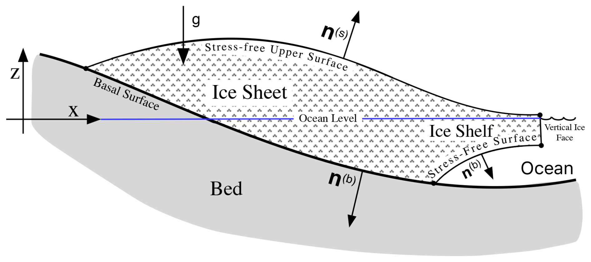
Referring to Fig. 1, the entire surface of the ice sheet is denoted by S. An upper surface, labeled S_S and specified by ${\mathit{\varsigma }}_s\left(x,y,z\right)=z-z_s\left(x,y\right)=\mathrm{0}$, is exposed to the atmosphere and thus experiences stress-free boundary conditions. The bottom or basal surface, denoted by S_B and specified by ${\mathit{\varsigma }}_b\left(x,y,z\right)=z-z_b\left(x,y\right)=\mathrm{0}$, is in contact with the bed. The basal surface may be subdivided into two sections, $S_B=S_{B\mathrm{1}}\cup S_{B\mathrm{2}}$, where S_B1, specified by $z=z_{b\mathrm{1}}\left(x,y\right)$, is the part where ice is frozen to the bed (a no-slip boundary condition), and S_B2, specified by $z=z_{b\mathrm{2}}\left(x,y\right)$, is where frictional sliding occurs. We assume Cartesian coordinates such that $x_i=\left(x,y,z\right)$ are position coordinates with z=0 at the ocean surface, and the index $i\in \left\{x,y,z\right\}$ represents the three Cartesian indices. Later we shall have occasion to introduce the restricted index $\left(i\right)\in \left\{x,y\right\}$ to represent just the two horizontal indices. This is more compact than the equivalent projection operator, i.e., $u_{\left(i\right)}=P_i\left(u\right)=\left(u,v,\mathrm{0}\right)$. Unit normal vectors appropriate for the ice sheet configuration of Fig. 1 are given by

$$\begin{array}{}\text{(1)}& \begin{array}{rl}& n_i=\left(n_x,n_y,n_z\right)={\displaystyle \frac{\partial {\mathit{\varsigma }}_s\left(x,y,z\right)/\partial x_i}{\left|\partial {\mathit{\varsigma }}_s\left(x,y,z\right)/\partial x_i\right|}}\\ & ={\displaystyle \frac{\left(-\partial z_s/\partial x,-\partial z_s/\partial y,\mathrm{1}\right)}{\sqrt{\mathrm{1}+{\left(\partial z_s/\partial x\right)}^{\mathrm{2}}+{\left(\partial z_s/\partial y\right)}^{\mathrm{2}}}}}\text{at surface}{S}_S,\\ & n_i=\left(n_x,n_y,n_z\right)=-{\displaystyle \frac{\partial {\mathit{\varsigma }}_b\left(x,y,z\right)/\partial x_i}{\left|\partial {\mathit{\varsigma }}_b\left(x,y,z\right)/\partial x_i\right|}}\\ & ={\displaystyle \frac{\left(\partial z_b/\partial x,\partial z_b/\partial y,-\mathrm{1}\right)}{\sqrt{\mathrm{1}+{\left(\partial z_b/\partial x\right)}^{\mathrm{2}}+{\left(\partial z_b/\partial y\right)}^{\mathrm{2}}}}}\text{at surface}{S}_B.\end{array}\end{array}$$

2.2 The Stokes equations

The Stokes model is a system of nonlinear partial differential equations and associated boundary conditions (Greve and Blatter, 2009; DPL10). In Cartesian coordinates the Stokes equations, the three momentum equations, and the continuity equation for the three velocity components $u_i=\left(u,v,w\right)$ and the pressure P are given by

$$\begin{array}{}\text{(2)}& {\displaystyle \frac{\partial {\mathit{\tau }}_{ij}}{\partial x_j}}-{\displaystyle \frac{\partial P}{\partial x_i}}+\mathit{\rho }{g}_i=\mathrm{0},\text{(3)}& {\displaystyle \frac{\partial u_i}{\partial x_i}}=\mathrm{0},\end{array}$$

where ρ is the density, and g_i is the acceleration vector due to gravity, arbitrarily oriented in general but here taken to be in the negative z direction, $g_i=\left(\mathrm{0},\mathrm{0},-g\right)$. Repeated indices imply summation (the Einstein notation). The deviatoric stress tensor τ_ij is given by

$$\begin{array}{}\text{(4)}& {\mathit{\tau }}_{ij}=\mathrm{2}{\mathit{\mu }}_n{\dot{\mathit{\epsilon }}}_{ij},\end{array}$$

where the strain rate tensor is

$$\begin{array}{}\text{(5)}& {\dot{\mathit{\epsilon }}}_{ij}={\displaystyle \frac{\mathrm{1}}{\mathrm{2}}}\left({\displaystyle \frac{\partial u_i}{\partial x_j}}+{\displaystyle \frac{\partial u_j}{\partial x_i}}\right),\end{array}$$

the nonlinear ice viscosity μ_n is

$$\begin{array}{}\text{(6)}& {\mathit{\mu }}_n={\mathit{\eta }}_{\mathrm{0}}{\left({\dot{\mathit{\epsilon }}}^{\mathrm{2}}\right)}^{(\mathrm{1}-n)/\mathrm{2}n},\end{array}$$

and ${\dot{\mathit{\epsilon }}}^{\mathrm{2}}={\dot{\mathit{\epsilon }}}_{ij}{\dot{\mathit{\epsilon }}}_{ij}/\mathrm{2}\ge \mathrm{0}$ is the second invariant of the strain rate tensor that may be written out in full as follows:

$$\begin{array}{}\text{(7)}& \begin{array}{rl}{\dot{\mathit{\epsilon }}}^{\mathrm{2}}& ={\displaystyle \frac{\mathrm{1}}{\mathrm{2}}}\left[{\left({\displaystyle \frac{\partial u}{\partial x}}\right)}^{\mathrm{2}}+{\left({\displaystyle \frac{\partial v}{\partial y}}\right)}^{\mathrm{2}}+{\left({\displaystyle \frac{\partial w}{\partial z}}\right)}^{\mathrm{2}}\right]\\ & +{\displaystyle \frac{\mathrm{1}}{\mathrm{4}}}\left[{\left({\displaystyle \frac{\partial u}{\partial y}}+{\displaystyle \frac{\partial v}{\partial x}}\right)}^{\mathrm{2}}+{\left({\displaystyle \frac{\partial u}{\partial z}}+{\displaystyle \frac{\partial w}{\partial x}}\right)}^{\mathrm{2}}+{\left({\displaystyle \frac{\partial v}{\partial z}}+{\displaystyle \frac{\partial w}{\partial y}}\right)}^{\mathrm{2}}\right].\end{array}\end{array}$$

As usual, ice is assumed to obey Glen's flow law, where n is Glen's law exponent (n=1 for a linear Newtonian fluid but typically n=3 in ice sheet modeling, describing a nonlinear non-Newtonian fluid). The coefficient η₀ is defined by ${\mathit{\eta }}_{\mathrm{0}}=A^{-\mathrm{1}/n}/\mathrm{2}$, where A is an ice flow factor, in general depending on temperature and other variables (see Schoof and Hewitt, 2013) but here taken to be a constant. The three-dimensional Stokes system requires a set of boundary conditions at every bounding surface, with each set composed of three components. Aside from the periodic lateral boundary conditions, the relevant boundary conditions are given as follows:

1. Stress-free boundary conditions on surfaces S_S not in contact with the bed, such as the upper surface S_S:

   $$\begin{array}{}\text{(8)}& {\mathit{\tau }}_{ij}{n}_j-P{n}_t=\mathrm{0}.\end{array}$$

2. No-slip or frozen to the bed conditions on surface segment S_B1:

   $$\begin{array}{}\text{(9)}& u_i=\mathrm{0}.\end{array}$$

3. Frictional tangential sliding conditions on surface segment S_B2.

We assume that the tangential frictional shear force that resists sliding, ${\mathit{\tau }}_i^S$, is a known vector that satisfies the no-penetration condition, ${\mathit{\tau }}_i^S{n}_i=\mathrm{0}$. Note that only two components need to be provided since the third may always be obtained from the tangency condition. In general ${\mathit{\tau }}_i^S$ is a complicated function of position and velocity (e.g., Schoof, 2010). At a surface where frictional sliding takes place the flow velocity must be tangential to the surface, satisfying

$$\begin{array}{}\text{(10)}& u_i{n}_i=\mathrm{0}.\end{array}$$

Following DPL10, the tangential stress balance at the basal surface is given by

$$\begin{array}{}\text{(11)}& {\mathit{\tau }}_{ij}{n}_j-{\mathit{\tau }}_n{n}_i+{\mathit{\tau }}_i^S=\mathrm{0},\end{array}$$

where τ_n=n_iτ_ijn_j is the normal component of the shear stress. However, the three components of the stress balance (11) are not independent since the stress balance vector is confined to the tangential plane. Thus, choosing the horizontal components of (11) as the two independent components, the required three boundary conditions are given by the no-penetration condition (10) and the two horizontal components of (11), namely

$$\begin{array}{}\text{(12)}& {\mathit{\tau }}_{\left(i\right)j}{n}_j-{\mathit{\tau }}_n{n}_{\left(i\right)}+{\mathit{\tau }}_{\left(i\right)}^S=\mathrm{0}.\end{array}$$

In this paper we shall assume simple linear frictional sliding, given by

$$\begin{array}{}\text{(13)}& {\mathit{\tau }}_i^S=\mathit{\beta }\left(x\right)u_i,\end{array}$$

where β(x)>0 is a position-dependent drag law coefficient. We also assume that there is no melting or refreezing at the bed, causing vertical inflows or outflows. If needed, these can be easily added to (10) (see DPL10; Heinlein et al., 2022).

2.3 The Stokes variational principle

A variational principle, if available, is the most compact way of representing a particular problem. It is fortunate that the Stokes model possesses a variational principle that is particularly useful for discretization and for the specification of boundary conditions – see Colinge and Rappaz (1999), Glowinski and Rappaz (2003), and Rappaz and Reist (2005) for early use of the variational principle in glaciology and Schoof (2006) and DPL10 for a fuller description of the variational principle as applied in ice sheet modeling. There are a number of significant advantages. For example, all boundary conditions are conveniently incorporated in the variational formulation, terms in the variational functional generally contain lower-order derivatives, and the discretization automatically generates a symmetric matrix. Stress terms are evaluated in the interior, thereby avoiding the need to evaluate derivatives using less accurate one-sided approximations at boundaries. Stress-free boundary conditions, as at the upper surface, need not be specified at all since they are automatically incorporated in the functional as natural boundary conditions. Finally, functional variation in the discrete case is equivalent to simple differentiation with respect to the discrete variables as demonstrated in Sect. 4. The variational method presented here is closely related to the Galerkin method, a subset of the weak formulation method in finite elements in which the test and trial functions are the same (see Schoof, 2010, and earlier references contained therein in connection with the Blatter–Pattyn model).

The variational functional for the standard Stokes model may be written in two alternative forms:

1. Basal boundary conditions imposed using Lagrange multipliers.

   $$\begin{array}{}\text{(14)}& \begin{array}{rl}A& [u_i,P,{\mathit{\lambda }}_i,\mathrm{\Lambda }]=\underset{V}{\int }dV\\ & \times \left[{\displaystyle \frac{\mathrm{4}n}{n+\mathrm{1}}}{\mathit{\eta }}_{\mathrm{0}}{\left({\dot{\mathit{\epsilon }}}^{\mathrm{2}}\right)}^{\left(\mathrm{1}+n\right)/\mathrm{2}n}-P{\displaystyle \frac{\partial u_i}{\partial x_i}}+\mathit{\rho }gw\right]\\ & +\underset{S_{B\mathrm{1}}}{\int }dS{\mathit{\lambda }}_i{u}_i+\underset{S_{B\mathrm{2}}}{\int }dS\left[\mathrm{\Lambda }{u}_i{n}_i+{\displaystyle \frac{\mathrm{1}}{\mathrm{2}}}\mathit{\beta }\left(x\right)u_i{u}_i\right],\end{array}\end{array}$$

   where λ_i and Λ are Lagrange multipliers used to enforce the no-slip condition and frictional tangential sliding, respectively. As in DPL10, arguments enclosed in square brackets, here $u_i,P,{\mathit{\lambda }}_i,\mathrm{\Lambda }$, indicate the functions that are subject to variation.

2. Basal boundary conditions imposed by direct substitution.

   In case of no-slip conditions, condition (9) is used directly in the functional to zero out all velocity components u_i along the S_B1 section of the basal boundary. In case of tangential sliding, the functional is given by

   $$\begin{array}{}\text{(15)}& \begin{array}{rl}A& [u_i,P]=\underset{V}{\int }dV\\ & \times \left[{\displaystyle \frac{\mathrm{4}n}{n+\mathrm{1}}}{\mathit{\eta }}_{\mathrm{0}}{\left({\dot{\mathit{\epsilon }}}^{\mathrm{2}}\right)}^{\left(\mathrm{1}+n\right)/\mathrm{2}n}-P{\displaystyle \frac{\partial u_i}{\partial x_i}}+\mathit{\rho }gw\right]\\ & +{\displaystyle \frac{\mathrm{1}}{\mathrm{2}}}\underset{S_{B\mathrm{2}}}{\int }dS\mathit{\beta }\left(x\right)\left(u_{\left(i\right)}{u}_{\left(i\right)}+{\left(u_{\left(i\right)}{n}_{\left(i\right)}/n_z\right)}^{\mathrm{2}}\right),\end{array}\end{array}$$

   where, using the tangential sliding condition (10), the velocity along the entire basal boundary section S_B2 is specified by

   $$\begin{array}{}\text{(16)}& u_i=\left(u,v,-u_{\left(i\right)}{n}_{\left(i\right)}/n_z\right)=\left(u,v,u_{\left(i\right)}\partial z_b/\partial x_{\left(i\right)}\right).\end{array}$$

   This is implicitly done in all terms of the functional, i.e., the volume integral terms as well as the surface integral term, in which case the replacement is explicitly visible in (15). This use of (16) to replace the relevant surface velocities in the functional is sufficient to implement the tangential sliding boundary condition. This replacement is particularly easy in the discrete formulation, to be described later, where boundary or surface velocity variables are easily accessible for replacement.

As described in DPL10, a variational procedure yields the full set of Euler–Lagrange equations and boundary conditions that specify the standard Stokes model, equivalent to (2)–(12). Using Lagrange multipliers, (14), the discrete variational procedure determines the discrete variables that specify the velocity components and the pressure, u_i and P, and the Lagrange multipliers, λ_i,Λ. In the direct substitution case, (15), the solution determines only the discrete pressures P and velocity variables u_i that were not directly prescribed as boundary conditions in (9) or (16). These prescribed (known) values of boundary velocities are then added a posteriori to obtain the complete set of discrete variables. The direct substitution method is more compact and simpler and therefore has been more commonly used in this paper.

3 A transformation of the Stokes model

3.1 Origin of the transformation

The transformation is motivated by the Blatter–Pattyn approximation. Consider the vertical component of the momentum equation and the corresponding stress-free upper surface boundary condition in the Blatter–Pattyn approximation (from DPL10, for example), which are given by

$$\begin{array}{}\text{(17)}& \begin{array}{l}\frac{\partial }{\partial z}\left(\mathrm{2}{\mathit{\mu }}_n\frac{\partial w}{\partial z}\right)-\frac{\partial P}{\partial z}-\mathit{\rho }g=\mathrm{0},\\ \left(\mathrm{2}{\mathit{\mu }}_n\frac{\partial w}{\partial z}-P\right)n_z=\mathrm{0}\text{at}z=z_s\left(x,y\right).\end{array}\end{array}$$

These equations suggest the use of a new variable $\stackrel{\mathrm{̃}}{P}$, to be called the transformed pressure, given by

$$\begin{array}{}\text{(18)}& \stackrel{\mathrm{̃}}{P}=P-\mathrm{2}{\mathit{\mu }}_n{\displaystyle \frac{\partial w}{\partial z}}+\mathit{\rho }g\left(z-z_s\left(x,y\right)\right).\end{array}$$

Using this, (17) simplifies as follows:

$$\begin{array}{}\text{(19)}& \begin{array}{l}\frac{\partial \stackrel{\mathrm{̃}}{P}}{\partial z}=\mathrm{0},\\ \stackrel{\mathrm{̃}}{P}{n}_z=\mathrm{0}\text{at}z=z_s\left(x,y\right),\end{array}\end{array}$$

which is a complete one-dimensional partial differential system that yields

$$\begin{array}{}\text{(20)}& \stackrel{\mathrm{̃}}{P}=\mathrm{0}\end{array}$$

when integrated from the top surface down. Thus, the transformed pressure vanishes in the Blatter–Pattyn case. Replacing the pressure P by $\stackrel{\mathrm{̃}}{P}$ by the use of (18) forms the basis of the present transformation, but we also make use of the continuity equation to eliminate $\partial w/\partial z$ as in the Blatter–Pattyn approximation (e.g., Pattyn, 2003). Thus, the transformation consists of eliminating P and $\partial w/\partial z$ in the Stokes system (2) and (4)–(12) (i.e., everywhere except in the continuity equation itself) by use of

$$\begin{array}{}\text{(21)}& P=\stackrel{\mathrm{̃}}{P}-\mathrm{2}{\mathit{\mu }}_n\left({\displaystyle \frac{\partial u}{\partial x}}+{\displaystyle \frac{\partial v}{\partial y}}\right)+\mathit{\rho }g\left(z_s-z\right),\end{array}$$

$$\begin{array}{}\text{(22)}& {\displaystyle \frac{\partial w}{\partial z}}=-\left({\displaystyle \frac{\partial u}{\partial x}}+{\displaystyle \frac{\partial v}{\partial y}}\right).\end{array}$$

The pressure P in the standard Stokes system is primarily a Lagrange multiplier enforcing incompressibility but with a very large hydrostatic component. The transformed pressure $\stackrel{\mathrm{̃}}{P}$ again acts as a Lagrange multiplier enforcing incompressibility. However, the transformation eliminates the hydrostatic pressure from $\stackrel{\mathrm{̃}}{P}$, making it some 3 orders of magnitude smaller than P as illustrated in Fig. 2. Since $\stackrel{\mathrm{̃}}{P}=\mathrm{0}$ in the Blatter–Pattyn approximation, the transformed pressure may be written as $\stackrel{\mathrm{̃}}{P}=P-P_{\mathrm{BP}}$, where

$$P_{\mathrm{BP}}=-\mathrm{2}{\mathit{\mu }}_n\left({\displaystyle \frac{\partial u}{\partial x}}+{\displaystyle \frac{\partial v}{\partial y}}\right)+\mathit{\rho }g\left(z_s-z\right)$$

is the effective Blatter–Pattyn pressure (Tezaur et al., 2015). Thus, $P=P_{\mathrm{BP}}+\stackrel{\mathrm{̃}}{P}$ and therefore $\stackrel{\mathrm{̃}}{P}$ may be interpreted as the “Stokes” correction to the Blatter–Pattyn pressure.

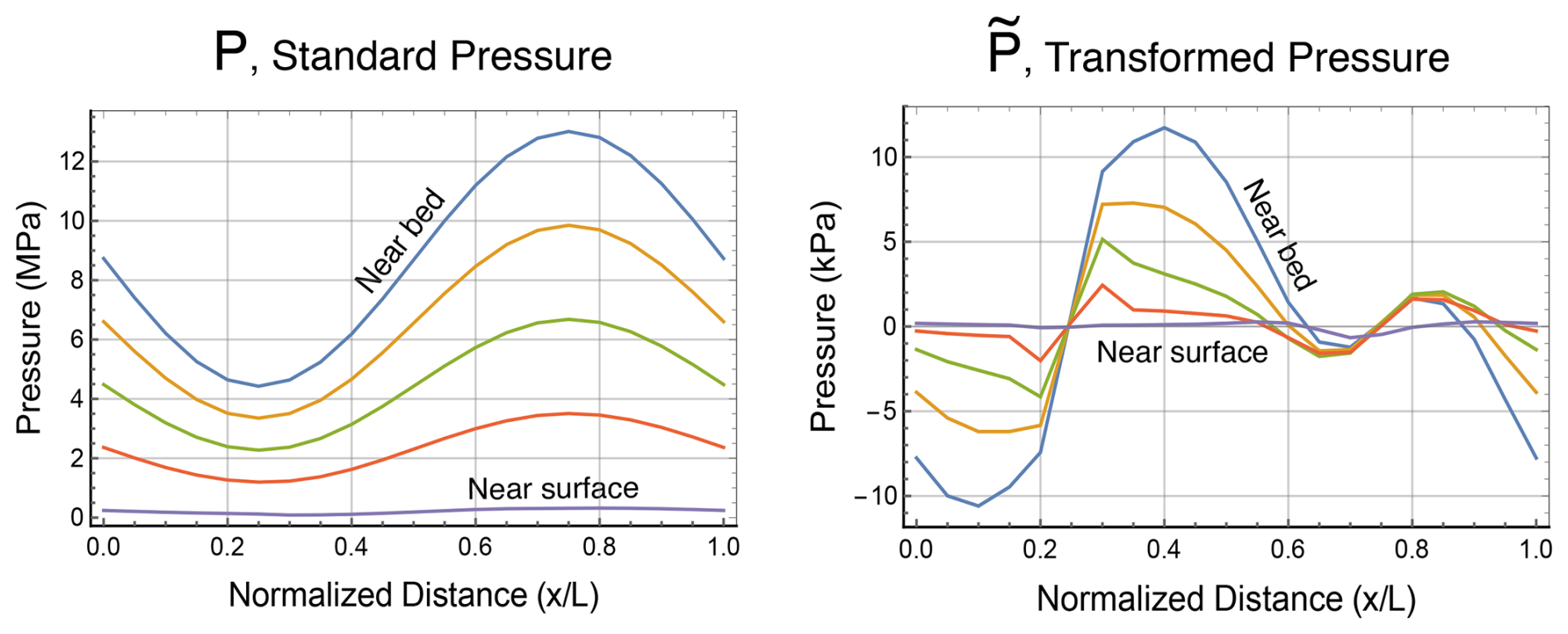
Figure 2 Standard pressure P (MPa) compared to the transformed pressure $\stackrel{\mathrm{̃}}{P}$ (kPa) in Exp. B from the ISMIP-HOM model intercomparison (Pattyn et al., 2008) at L=10 km.

3.2 The transformed Stokes equations

Introducing (21) and (22) into the Stokes system of Eqs. (2)–(12) results in the following transformed Stokes system:

$$\begin{array}{}\text{(23)}& {\displaystyle \frac{\partial {\stackrel{\mathrm{̃}}{\mathit{\tau }}}_{ij}}{\partial x_j}}-\widehat{\mathit{\xi }}{\displaystyle \frac{\partial \stackrel{\mathrm{̃}}{P}}{\partial x_i}}-\mathit{\rho }g{\displaystyle \frac{\partial z_s}{\partial x_{\left(i\right)}}}=\mathrm{0},\text{(24)}& {\displaystyle }\widehat{\mathit{\xi }}{\displaystyle \frac{\partial u_i}{\partial x_i}}=\mathrm{0},\end{array}$$

where quantities modified in the transformation are indicated by a tilde, e.g., $\stackrel{\mathrm{̃}}{P}$. Corresponding to (4), the modified Stokes deviatoric stress tensor ${\stackrel{\mathrm{̃}}{\mathit{\tau }}}_{ij}$ is given by

$$\begin{array}{}\text{(25)}& {\stackrel{\mathrm{̃}}{\mathit{\tau }}}_{ij}={\stackrel{\mathrm{̃}}{\mathit{\mu }}}_n\left[\begin{array}{lll}\mathrm{2}\left(\mathrm{2}\frac{\partial u}{\partial x}+\frac{\partial v}{\partial y}\right)& \left(\frac{\partial u}{\partial y}+\frac{\partial v}{\partial x}\right)& \left(\frac{\partial u}{\partial z}+\mathit{\xi }\frac{\partial w}{\partial x}\right)\\ \left(\frac{\partial u}{\partial y}+\frac{\partial v}{\partial x}\right)& \mathrm{2}\left(\frac{\partial u}{\partial x}+\mathrm{2}\frac{\partial v}{\partial y}\right)& \left(\frac{\partial v}{\partial z}+\mathit{\xi }\frac{\partial w}{\partial y}\right)\\ \mathit{\xi }\left(\frac{\partial u}{\partial z}+\frac{\partial w}{\partial x}\right)& \mathit{\xi }\left(\frac{\partial v}{\partial z}+\frac{\partial w}{\partial y}\right)& \mathrm{0}\end{array}\right].\end{array}$$

Dummy variables $\mathit{\xi },\widehat{\mathit{\xi }}$ (here assumed to be $\mathit{\xi },\widehat{\mathit{\xi }}=\mathrm{1})$ have been introduced to indicate terms that are absent in the Blatter–Blatter approximation, as will be more fully explained below. The modified viscosity ${\stackrel{\mathrm{̃}}{\mathit{\mu }}}_n$, corresponding to (6), is given by

$$\begin{array}{}\text{(26)}& {\stackrel{\mathrm{̃}}{\mathit{\mu }}}_n={\mathit{\eta }}_{\mathrm{0}}{\left({\stackrel{\mathrm{̃}}{\dot{\mathit{\epsilon }}}}^{\mathrm{2}}\right)}^{(\mathrm{1}-n)/\mathrm{2}n},\end{array}$$

where the transformed second invariant ${\stackrel{\mathrm{̃}}{\dot{\mathit{\epsilon }}}}^{\mathrm{2}}$, corresponding to (7), is

$$\begin{array}{}\text{(27)}& \begin{array}{rl}{\stackrel{\mathrm{̃}}{\dot{\mathit{\epsilon }}}}^{\mathrm{2}}& ={\left({\displaystyle \frac{\partial u}{\partial x}}\right)}^{\mathrm{2}}+{\displaystyle \frac{\partial u}{\partial x}}{\displaystyle \frac{\partial v}{\partial y}}+{\left({\displaystyle \frac{\partial v}{\partial y}}\right)}^{\mathrm{2}}+{\displaystyle \frac{\mathrm{1}}{\mathrm{4}}}\left[{\left({\displaystyle \frac{\partial u}{\partial y}}+{\displaystyle \frac{\partial v}{\partial x}}\right)}^{\mathrm{2}}\right.\\ & \left.+{\left({\displaystyle \frac{\partial u}{\partial z}}+\mathit{\xi }{\displaystyle \frac{\partial w}{\partial x}}\right)}^{\mathrm{2}}+{\left({\displaystyle \frac{\partial v}{\partial z}}+\mathit{\xi }{\displaystyle \frac{\partial w}{\partial y}}\right)}^{\mathrm{2}}\right].\end{array}\end{array}$$

Since (27) differs from (7) only by the incorporation of the continuity equation (22), the transformation leaves both the second invariant ${\stackrel{\mathrm{̃}}{\dot{\mathit{\epsilon }}}}^{\mathrm{2}}$ and viscosity ${\stackrel{\mathrm{̃}}{\mathit{\mu }}}_n$ unchanged, i.e., ${\stackrel{\mathrm{̃}}{\dot{\mathit{\epsilon }}}}^{\mathrm{2}}={\dot{\mathit{\epsilon }}}^{\mathrm{2}}$ and ${\stackrel{\mathrm{̃}}{\mathit{\mu }}}_n={\mathit{\mu }}_n$, which also implies that ${\stackrel{\mathrm{̃}}{\dot{\mathit{\epsilon }}}}^{\mathrm{2}}\ge \mathrm{0}$.

Boundary conditions for the transformed equations, corresponding to (8)–(12), are given by

$$\begin{array}{}\text{(28)}& {\displaystyle }\text{BCs on}{S}_S:{\stackrel{\mathrm{̃}}{\mathit{\tau }}}_{ij}{n}_j-\widehat{\mathit{\xi }}\stackrel{\mathrm{̃}}{P}{n}_i=\mathrm{0},\text{(29)}& {\displaystyle }\text{BCs on}{S}_{B\mathrm{1}}:u_i=\mathrm{0},\text{(30)}& {\displaystyle }\text{BCs on}{S}_{B\mathrm{2}}:u_i{n}_i=\mathrm{0},\text{(31)}& {\displaystyle }{\stackrel{\mathrm{̃}}{\mathit{\tau }}}_{\left(i\right)j}{n}_j-{\stackrel{\mathrm{̃}}{\mathit{\tau }}}_n{n}_{\left(i\right)}+\mathit{\beta }\left(x\right)u_{\left(i\right)}=\mathrm{0},\end{array}$$

where ${\stackrel{\mathrm{̃}}{\mathit{\tau }}}_n=n_i{\stackrel{\mathrm{̃}}{\mathit{\tau }}}_{ij}{n}_j$ as before. Equations (30) and (31) constitute the required three frictional sliding boundary conditions.

As mentioned, dummy variables $\mathit{\xi },\widehat{\mathit{\xi }}$ in (23)–(25), (27), and (28) are used to identify terms that are neglected in the two types of the Blatter–Pattyn approximation discussed in Sect. 3.4. These are (a) the standard Blatter–Pattyn approximation, $\mathit{\xi }=\mathrm{0},\widehat{\mathit{\xi }}=\mathrm{0}$, as originally derived (Blatter, 1995; Pattyn, 2003; DPL10), which solves for just the horizontal velocity components u,v, and (b) the extended Blatter–Pattyn approximation, $\mathit{\xi }=\mathrm{0},\widehat{\mathit{\xi }}=\mathrm{1}$, described more fully in Sect. 3.4.2, which contains the standard approximation plus additional equations that determine the vertical velocity w and the pressure $\stackrel{\mathrm{̃}}{P}$. Retaining all terms, i.e., $\mathit{\xi }=\mathrm{1},\widehat{\mathit{\xi }}=\mathrm{1}$, specifies the full transformed Stokes model.

The transformed system, (23)–(31), and the standard Stokes system, (2)–(12), produce exactly the same solution. However, in common with the Blatter–Pattyn approximation, the transformed system requires the use a gravity-oriented coordinate system because of the particular type of gravitational forcing being used, while the standard Stokes model is not similarly restricted. This is not a major limitation. Somewhat more restrictive is the appearance of z_s(x,y), an implicitly single valued function, to describe the vertical position of the upper surface of the ice sheet. This means that care must be taken with reentrant upper surfaces (i.e., S-shaped in 2D) and sloping cliffs at an ice edge – again a restriction that is not present in the standard Stokes model. As noted earlier, we assume that there is just one upper and one basal surface; i.e., as usual in ice sheet modeling this does not permit overhangs.

3.3 The transformed Stokes variational principle

It is easy to verify that the transformed Stokes system (23)–(31) results from the variation with respect to $u_i,\stackrel{\mathrm{̃}}{P}$ of the following functional:

$$\begin{array}{}\text{(32)}& \begin{array}{rl}\stackrel{\mathrm{̃}}{A}& [u_i,\stackrel{\mathrm{̃}}{P}]=\underset{V}{\int }dV\\ & \times \left[{\displaystyle \frac{\mathrm{4}n}{n+\mathrm{1}}}{\mathit{\eta }}_{\mathrm{0}}{\left({\stackrel{\mathrm{̃}}{\dot{\mathit{\epsilon }}}}^{\mathrm{2}}\right)}^{\left(\mathrm{1}+n\right)/\mathrm{2}n}-\widehat{\mathit{\xi }}\stackrel{\mathrm{̃}}{P}{\displaystyle \frac{\partial u_i}{\partial x_i}}+\mathit{\rho }g{u}_{\left(i\right)}{\displaystyle \frac{\partial z_s}{\partial x_{\left(i\right)}}}\right]\\ & +{\displaystyle \frac{\mathrm{1}}{\mathrm{2}}}\underset{S_{B\mathrm{2}}}{\int }dS\mathit{\beta }\left(x\right)\left(u_{\left(i\right)}{u}_{\left(i\right)}+{\left(u_{\left(i\right)}{n}_{\left(i\right)}/n_z\right)}^{\mathrm{2}}\right),\end{array}\end{array}$$

where ${\stackrel{\mathrm{̃}}{\dot{\mathit{\epsilon }}}}^{\mathrm{2}}$ is the transformed second invariant, (27). As in functional (15), here basal boundary conditions are imposed by direct substitution. However, using Lagrange multipliers as in (14) is also possible.

3.4 Two forms of the Blatter–Pattyn approximation

3.4.1 The standard Blatter–Pattyn approximation

The standard Blatter–Pattyn approximation (originally introduced by Blatter, 1995, and Pattyn, 2003, and later by DPL10, and Schoof and Hewitt, 2013) is obtained by setting $\mathit{\xi }=\widehat{\mathit{\xi }}=\mathrm{0}$ in the transformed system. This yields the Blatter–Pattyn functional,

$$\begin{array}{}\text{(33)}& \begin{array}{rl}{A}_{\mathrm{BP}}& \left[u_{\left(i\right)}\right]=\underset{V}{\int }dV\\ & \times \left[{\displaystyle \frac{\mathrm{4}n}{n+\mathrm{1}}}{\mathit{\eta }}_{\mathrm{0}}{\left({\dot{\mathit{\epsilon }}}_{\mathrm{BP}}^{\mathrm{2}}\right)}^{\left(\mathrm{1}+n\right)/\mathrm{2}n}+\mathit{\rho }g{u}_{\left(i\right)}{\displaystyle \frac{\partial z_s}{\partial x_{\left(i\right)}}}\right]\\ & +{\displaystyle \frac{\mathrm{1}}{\mathrm{2}}}\underset{S_{B\mathrm{2}}}{\int }dS\mathit{\beta }\left(x\right)\left(u_{\left(i\right)}{u}_{\left(i\right)}+\mathit{\varsigma }{\left(u_{\left(i\right)}{n}_{\left(i\right)}/n_z\right)}^{\mathrm{2}}\right),\end{array}\end{array}$$

and the second invariant,

$$\begin{array}{}\text{(34)}& \begin{array}{rl}{\dot{\mathit{\epsilon }}}_{\mathrm{BP}}^{\mathrm{2}}& ={\left({\displaystyle \frac{\partial u}{\partial x}}\right)}^{\mathrm{2}}+{\displaystyle \frac{\partial u}{\partial x}}{\displaystyle \frac{\partial v}{\partial y}}+{\left({\displaystyle \frac{\partial v}{\partial y}}\right)}^{\mathrm{2}}\\ & +{\displaystyle \frac{\mathrm{1}}{\mathrm{4}}}\left[{\left({\displaystyle \frac{\partial u}{\partial y}}+{\displaystyle \frac{\partial v}{\partial x}}\right)}^{\mathrm{2}}+{{\displaystyle \frac{\partial u}{\partial z}}}^{\mathrm{2}}+{{\displaystyle \frac{\partial v}{\partial z}}}^{\mathrm{2}}\right],\end{array}\end{array}$$

in terms of horizontal velocity components u,v only. The Euler–Lagrange equations and boundary conditions are given by

$$\begin{array}{}\text{(35)}& \begin{array}{rl}& {\displaystyle \frac{\partial {\mathit{\tau }}_{\left(i\right)j}^{\mathrm{BP}}}{\partial x_j}}-\mathit{\rho }g{\displaystyle \frac{\partial z_s}{\partial x_{\left(i\right)}}}=\mathrm{0};\\ & \left\{\begin{array}{c}{\mathit{\tau }}_{\left(i\right)j}^{\mathrm{BP}}{n}_j+\mathit{\beta }\left(x\right)\left(u_{\left(i\right)}+\mathit{\zeta }\left(u_{\left(j\right)}{n}_{\left(j\right)}/n_z\right)n_{\left(i\right)}/n_z\right)=\mathrm{0}\\ \text{on}{S}_{B\mathrm{2}},{\mathit{\tau }}_{\left(i\right)j}^{\mathrm{BP}}{n}_j=\mathrm{0}\text{on}{S}_S,u_{\left(i\right)}=\mathrm{0}\text{on}{S}_{\mathrm{B}\mathrm{1}},\end{array}\right.\end{array}\end{array}$$

where the Blatter–Pattyn stress tensor ${\mathit{\tau }}_{\left(i\right)j}^{\mathrm{BP}}$ is

$$\begin{array}{}\text{(36)}& {\mathit{\tau }}_{\left(i\right)j}^{\mathrm{BP}}={\stackrel{\mathrm{̃}}{\mathit{\mu }}}_n^{\mathrm{BP}}\left[\begin{array}{lll}\mathrm{2}\left(\mathrm{2}\frac{\partial u}{\partial x}+\frac{\partial v}{\partial y}\right)& \left(\frac{\partial u}{\partial y}+\frac{\partial v}{\partial x}\right)& \frac{\partial u}{\partial z}\\ \left(\frac{\partial u}{\partial y}+\frac{\partial v}{\partial x}\right)& \mathrm{2}\left(\frac{\partial u}{\partial x}+\mathrm{2}\frac{\partial v}{\partial y}\right)& \frac{\partial v}{\partial z}\end{array}\right],\end{array}$$

and ${\stackrel{\mathrm{̃}}{\mathit{\mu }}}_n^{\mathrm{BP}}={\mathit{\eta }}_{\mathrm{0}}{\left({\stackrel{\mathrm{̃}}{\dot{\mathit{\epsilon }}}}_{\mathrm{BP}}^{\mathrm{2}}\right)}^{(\mathrm{1}-n)/\mathrm{2}n}$. A new dummy variable ζ has been introduced in (33) to identify the basal boundary term normally dropped in the standard Blatter–Pattyn approximation (ζ=0) but restored (ζ=1) in Dukowicz et al. (2011) to better represent arbitrary basal topography.

The Blatter–Pattyn model solves for the horizontal velocity components only. In principle the vertical velocity component w may be computed a posteriori by means of the continuity equation, if desired. It is important to note that the Blatter–Pattyn system is numerically well behaved because its variational formulation amounts to a convex optimization problem whose solution minimizes the functional (33).

3.4.2 The extended Blatter–Pattyn approximation

A second form of the Blatter–Pattyn approximation is obtained from the transformed variational principle (32) by making the assumption

$$\begin{array}{}\text{(37)}& ∥{\displaystyle \frac{\partial w}{\partial x}}∥\ll ∥{\displaystyle \frac{\partial u}{\partial z}}∥,∥{\displaystyle \frac{\partial w}{\partial y}}∥\ll ∥{\displaystyle \frac{\partial v}{\partial z}}∥\end{array}$$

and therefore neglecting $\partial w/\partial x,\partial w/\partial y$ in the transformed second invariant ${\stackrel{\mathrm{̃}}{\dot{\mathit{\epsilon }}}}^{\mathrm{2}}$, consistent with the original small aspect ratio approximation (Blatter, 1995; Pattyn, 2003; DPL10; Schoof and Hindmarsh, 2010). This corresponds to setting $\mathit{\xi }=\mathrm{0},\widehat{\mathit{\xi }}=\mathrm{1}$ in the transformed Stokes model. In other words, we neglect w-velocity gradients in the second invariant but keep the pressure term in the functional. This will be called the extended Blatter–Pattyn approximation (EBP) because, in contrast to the standard Blatter–Pattyn approximation, all the variables, i.e., $u,v,w,\stackrel{\mathrm{̃}}{P}$, are retained. It is noteworthy that assumption (37) is equivalent to just setting w=0 in the second invariant ${\stackrel{\mathrm{̃}}{\dot{\mathit{\epsilon }}}}^{\mathrm{2}}$ in the transformed Stokes model. This will be exploited later to obtain approximations that improve on the Blatter–Pattyn approximation. Thus, the extended Blatter–Pattyn functional is given by

$$\begin{array}{}\text{(38)}& \begin{array}{rl}{A}_{\mathrm{EBP}}& [u_i,\stackrel{\mathrm{̃}}{P}]=\underset{V}{\int }dV\\ & \times \left[{\displaystyle \frac{\mathrm{4}n}{n+\mathrm{1}}}{\mathit{\eta }}_{\mathrm{0}}{\left({\dot{\mathit{\epsilon }}}_{\mathrm{BP}}^{\mathrm{2}}\right)}^{\left(\mathrm{1}+n\right)/\mathrm{2}n}-\stackrel{\mathrm{̃}}{P}{\displaystyle \frac{\partial u_i}{\partial x_i}}+\mathit{\rho }g{u}_{\left(i\right)}{\displaystyle \frac{\partial z_s}{\partial x_{\left(i\right)}}}\right]\\ & +{\displaystyle \frac{\mathrm{1}}{\mathrm{2}}}\underset{S_{B\mathrm{2}}}{\int }dS\mathit{\beta }\left(x\right)\left(u_{\left(i\right)}{u}_{\left(i\right)}+\mathit{\varsigma }{\left(u_{\left(i\right)}{n}_{\left(i\right)}/n_z\right)}^{\mathrm{2}}\right),\end{array}\end{array}$$

where the Blatter–Pattyn second invariant ${\dot{\mathit{\epsilon }}}_{\mathrm{BP}}^{\mathrm{2}}$ is given by (34). Taking the variation yields the system of extended Blatter–Pattyn and Euler–Lagrange equations and their boundary conditions as follows:

1. Variation with respect to u_(i) yields the horizontal momentum equation,

   $$\begin{array}{}\text{(39)}& \begin{array}{rl}& {\displaystyle \frac{\partial {\mathit{\tau }}_{\left(i\right)j}^{\mathrm{BP}}}{\partial x_j}}-{\displaystyle \frac{\partial \stackrel{\mathrm{̃}}{P}}{\partial x_{\left(i\right)}}}-\mathit{\rho }g{\displaystyle \frac{\partial z_s}{\partial x_{\left(i\right)}}}=\mathrm{0};\\ & \left\{\begin{array}{l}{\mathit{\tau }}_{\left(i\right)j}^{\mathrm{BP}}{n}_j-\stackrel{\mathrm{̃}}{P}{n}_{\left(i\right)}=\mathrm{0}\text{on}{S}_S,u_{\left(i\right)}=\mathrm{0}\text{on}{S}_{B\mathrm{1}},\\ \begin{array}{l}{\mathit{\tau }}_{\left(i\right)j}^{BP}{n}_j+\mathit{\beta }\left(x\right)\left(u_{\left(i\right)}+\mathit{\zeta }\left(u_{\left(k\right)}{n}_{\left(k\right)}/n_z\right)n_{\left(i\right)}/n_z\right)=\mathrm{0}\\ \text{on}{S}_{B\mathrm{2}},\end{array}\end{array}\right.\end{array}\end{array}$$

   where ${\mathit{\tau }}_{\left(i\right)j}^{\mathrm{BP}}$ is given by (36).

2. Variation with respect to w yields the vertical momentum equation,

   $$\begin{array}{}\text{(40)}& -{\displaystyle \frac{\partial \stackrel{\mathrm{̃}}{P}}{\partial z}}=\mathrm{0};\stackrel{\mathrm{̃}}{P}{n}_z=\mathrm{0}\text{on}{S}_S.\end{array}$$

3. Variation with respect to $\stackrel{\mathrm{̃}}{P}$ yields the continuity equation,

   $$\begin{array}{}\text{(41)}& \begin{array}{rl}{\displaystyle \frac{\partial w}{\partial z}}& +{\displaystyle \frac{\partial u_{\left(i\right)}}{\partial x_{\left(i\right)}}}=\mathrm{0};w=\mathrm{0}\text{on}{S}_{B\mathrm{1}},\\ & \text{or}w=-u_{\left(i\right)}{n}_{\left(i\right)}/n_z\text{on}{S}_{B\mathrm{2}}.\end{array}\end{array}$$

It is apparent that the vertical momentum equation system (40) is a decoupled system, yielding $\stackrel{\mathrm{̃}}{P}=\mathrm{0}$ as already shown in Sect. 3.1. This eliminates the pressure from the horizontal momentum equation (39), making it identical to the standard Blatter–Pattyn system (35), i.e., a decoupled system for the horizontal velocities u_(i). As a result, having solved (39) for the horizontal velocities, the continuity equation (41) may in principle be solved for the vertical velocity w (but see the comments regarding the discrete case that follow Eq. 42).

In summary, the extended Blatter–Pattyn model, (39)–(41), is equivalent to the standard Blatter–Pattyn model, (35), for the horizontal velocities, u,v, but it also includes two additional equations determining the pressure $\stackrel{\mathrm{̃}}{P}$ and the vertical velocity w that are ignored in the standard Blatter–Pattyn approximation. Because of this, we distinguish between the Blatter–Pattyn model that solves for just the two horizontal velocities (i.e., the standard Blatter–Pattyn approximation, Eq. 35) and the Blatter–Pattyn system that solves for all the variables (i.e., the extended Blatter–Pattyn approximation, Eqs. 39–41). Perhaps the main distinction between the two, which may be important in some applications, is that in the Blatter–Pattyn system the continuity equation (41) is solved for the vertical velocity w simultaneously with (39) for the horizontal velocities u,v on the same mesh, while in the Blatter–Pattyn model the calculation of vertical velocity is completely decoupled and may be done on an unrelated mesh. In the continuous case the solution for the vertical velocity can be done using Leibniz's theorem,

$$\begin{array}{}\text{(42)}& \begin{array}{rl}w\left(u,v\right)& =w_{z=z_b}-\underset{z_b}{\overset{z}{\int }}{\displaystyle \frac{\partial u_{\left(i\right)}}{\partial x_{\left(i\right)}}}d{z}^{\prime }=u_{\left(i\right)}{\displaystyle \frac{\partial z_b}{\partial x_{\left(i\right)}}}\\ & -\underset{z_b}{\overset{z}{\int }}{\displaystyle \frac{\partial u_{\left(i\right)}}{\partial x_{\left(i\right)}}}d{z}^{\prime }=-{\displaystyle \frac{\partial }{\partial x_{\left(i\right)}}}\underset{z_b}{\overset{z}{\int }}{u}_{\left(i\right)}d{z}^{\prime }.\end{array}\end{array}$$

Equation (42) may in principle be discretized to obtain the vertical velocity on arbitrary meshes. However, discretizations of the continuity Eq. (41) are generally not capable of being solved for the vertical velocity in terms of the horizontal velocities. In Appendix A we shall introduce special finite element meshes that do allow for the solvability of the discrete continuity equation for the vertical velocity.

Up to now we have only dealt with continuum properties of Stokes-type systems, which are well behaved. However, this may not be so in the discrete case. The solution of the discretized Stokes systems will depend on the choices that are made for the meshes and for the finite elements that are to be used. These issues will be discussed next.

4 Finite element discretization

4.1 Standard and transformed Stokes discretizations

In practice, both traditional Stokes and Blatter–Pattyn models are discretized using finite element methods (e.g., Gagliardini et al., 2013; Perego et al., 2012). We follow this practice except that here the discretization starts from the Stokes variational principle. This differs from standard finite element practice that begins with the Stokes equations and converts them into weak (integral) form, which may not be equivalent to a variational formulation unless the Galerkin method is used. A variational principle has a number of advantages (see Sect. 2.3 and DPL10). The following is a brief outline of the discretization. Additional details are provided in Appendix A. For simplicity, we confine ourselves to two dimensions with coordinates (x,z) and velocities (u,w). An example of a three-dimensional mesh appropriate for our purpose is discussed in Appendix A. Further, we discuss only the case of direct substitution for basal boundary conditions in the variational functional. Remarks will apply to both the standard and the transformed Stokes models. Thus, the discrete pressure variable p may refer to either the standard pressure P or the transformed pressure $\stackrel{\mathrm{̃}}{P}$.

Consider an arbitrary mesh with a total of $N=n_u+n_w+n_p$ unknown discrete variables at nodal locations $\mathrm{1}\le i\le N$, with n_u horizontal velocity variables, n_w vertical velocity variables, and n_p pressure variables, so that

$$\begin{array}{}\text{(43)}& \begin{array}{rl}\mathit{v}& ={\left\{v_{\mathrm{1}},v_{\mathrm{2}},\mathrm{\dots },v_N\right\}}^T=\left\{\left\{u_{\mathrm{1}},u_{\mathrm{2}},\mathrm{\dots },u_{n_u}\right\},\right.\\ & {\left.\left\{w_{\mathrm{1}},w_{\mathrm{2}},\mathrm{\dots },w_{n_w}\right\},\left\{p_{\mathrm{1}},p_{\mathrm{2}},\mathrm{\dots },p_{n_p}\right\}\right\}}^T={\left\{\mathit{u},\mathit{w},\mathit{p}\right\}}^T\end{array}\end{array}$$

is the vector of unknown discrete variables that are the degrees of freedom of the model (if using Lagrange multipliers for basal boundary conditions then discrete variables corresponding to λ_z,Λ must be added). Variables are expanded in terms of shape functions $N_i^k\left(\mathit{x}\right)$ associated with each nodal variable i in each element k, so that ${\mathit{v}}^k\left(\mathbf{x}\right)=\sum _i{v}_i{N}_i^k\left(\mathbf{x}\right)$ is the spatial variation of variables in element k, summed over all variable nodes located in element k. Shape functions associated with a given node may differ depending on the variable. Substituting into the functional, (15) or (32), integrating and assembling the contributions of all elements, we obtain a discretized variational functional in terms of the nodal variable vectors $\mathit{u},\mathit{w},\mathit{p}$, as follows:

$$\begin{array}{}\text{(44)}& A\left(\mathit{u},\mathit{w},\mathit{p}\right)=\sum _k{A}^k\left(\mathit{u},\mathit{w},\mathit{p}\right),\end{array}$$

where $A^k\left(\mathit{u},\mathit{w},\mathit{p}\right)$ is the local functional evaluated by integrating over element k. Since the product of pressure and the divergence of velocity in the functional is linear in pressure and velocity, and the term responsible for gravity forcing is linear in velocity, the functional (44) may be written in discrete form as follows:

$$\begin{array}{}\text{(45)}& \begin{array}{rl}A\left(\mathit{u},\mathit{w},\mathit{p}\right)& =M\left(\mathit{u},\mathit{w}\right)+{\mathit{p}}^T\left({\mathbf{M}}_{\mathrm{UP}}^T\mathit{u}+{\mathbf{M}}_{\mathrm{WP}}^T\mathit{w}\right)\\ & +{\mathit{u}}^T{\mathit{f}}_U+{\mathit{w}}^T{\mathit{f}}_W,\end{array}\end{array}$$

where the notation from (43) has been used, i.e., $\mathit{u}={\left\{u_{\mathrm{1}},u_{\mathrm{2}},\mathrm{\dots },u_{n_u}\right\}}^T$, etc. Parentheses indicate a functional dependence on the indicated variables. Comparison with (15) and (32) shows that $M\left(\mathit{u},\mathit{w}\right)\ge \mathrm{0}$ is a highly nonlinear function of the velocity variables u,w, and ${\mathbf{M}}_{\mathrm{UP}}^T$ and ${\mathbf{M}}_{\mathrm{WP}}^T$ are constant n_p×n_u and n_p×n_w matrices, respectively, arising from the incompressibility constraint. Note that f_U and f_W are constant gravity forcing vectors of dimension n_u and n_w, respectively, such that ${\mathit{f}}_U=\mathrm{0},{\mathit{f}}_W\ne \mathrm{0}$ in the standard Stokes model and ${\mathit{f}}_U\ne \mathrm{0},{\mathit{f}}_W=\mathrm{0}$ in the transformed Stokes model. The discrete functional M(u,w) differs in the two cases but remains positive-definite.

Variation of the discretized functional corresponds to partial differentiation with respect to each of the discrete variables in the vector v (see Eq. 43). Thus, the discrete Euler–Lagrange equations that correspond to the u-momentum, w-momentum, and continuity equations, respectively, are given by

$$\begin{array}{}\text{(46)}& \begin{array}{rl}\mathit{R}\left(\mathit{u},\mathit{w},\mathit{p}\right)& =\left[\begin{array}{l}\partial A\left(\mathit{u},\mathit{w},\mathit{p}\right)/\partial \mathit{u}\\ \partial A\left(\mathit{u},\mathit{w},\mathit{p}\right)/\partial \mathit{w}\\ \partial A\left(\mathit{u},\mathit{w},\mathit{p}\right)/\partial \mathit{p}\end{array}\right]=\left[\begin{array}{l}{\mathit{R}}_U\left(\mathit{u},\mathit{w},\mathit{p}\right)\\ {\mathit{R}}_W\left(\mathit{u},\mathit{w},\mathit{p}\right)\\ {\mathit{R}}_P\left(\mathit{u},\mathit{w}\right)\end{array}\right]\\ & =\left[\begin{array}{l}{M}_U\left(\mathit{u},\mathit{w}\right)+{\mathbf{M}}_{\mathrm{UP}}\mathit{p}+{\mathit{f}}_U\\ M_W\left(\mathit{u},\mathit{w}\right)+{\mathbf{M}}_{\mathrm{WP}}\mathit{p}+{\mathit{f}}_W\\ {\mathbf{M}}_{\mathrm{UP}}^{T}u+{\mathbf{M}}_{\mathrm{WP}}^T\mathit{w}\end{array}\right]=\mathrm{0},\end{array}\end{array}$$

where functionals $M_U\left(\mathit{u},\mathit{w}\right)=\partial M\left(\mathit{u},\mathit{w}\right)/\partial \mathit{u}$ and $M_W\left(\mathit{u},\mathit{w}\right)=\partial M\left(\mathit{u},\mathit{w}\right)/\partial \mathit{w}$ are nonlinear vectors of dimension n_u and n_w, respectively. Altogether, (46) is a set of N nonlinear equations for the N unknown discrete variables v_i. As explained previously in the continuum case, all boundary conditions are included in functional (45), and therefore they are also incorporated in the discrete Euler–Lagrange equations (46).

Since the overall system (46) is nonlinear, it is normally solved using the Newton–Raphson iteration, expressed in matrix notation as follows:

$$\begin{array}{}\text{(47)}& \mathbf{M}\left({\mathit{u}}^K,{\mathit{w}}^K\right)\mathrm{\Delta }\mathit{v}+\mathit{R}\left({\mathit{u}}^K,{\mathit{w}}^K,{\mathit{p}}^K\right)=\mathrm{0},\end{array}$$

where K is the iteration index, $\mathbf{M}\left(\mathit{u},\mathit{w}\right)={\partial }^{\mathrm{2}}A\left(\mathit{v}\right)/\partial v_i\partial v_j$ is a symmetric N×N Hessian matrix, and Δv is the column vector given by

$$\begin{array}{rl}\mathrm{\Delta }\mathit{v}& ={\left\{\mathrm{\Delta }\mathit{u},\mathrm{\Delta }\mathit{w},\mathrm{\Delta }\mathit{p}\right\}}^T\\ & ={\left\{{\mathit{u}}^{K+\mathrm{1}}-{\mathit{u}}^K,{\mathit{w}}^{K+\mathrm{1}}-{\mathit{w}}^K,{\mathit{p}}^{K+\mathrm{1}}-{\mathit{p}}^K\right\}}^T.\end{array}$$

Given v^K from the previous iteration, (47) is a linear matrix equation that is solved for the N new variables v^K+1 at each iteration. In view of (45) and (46), the Hessian matrix M(u,w) may be decomposed into submatrices as follows:

$$\begin{array}{}\text{(48)}& \mathbf{M}\left(\mathit{u},\mathit{w}\right)=\left[\begin{array}{lll}{\mathbf{M}}_{\mathrm{UU}}\left(\mathit{u},\mathit{w}\right)& {\mathbf{M}}_{\mathrm{UW}}\left(\mathit{u},\mathit{w}\right)& {\mathbf{M}}_{\mathrm{UP}}\\ {\mathbf{M}}_{\mathrm{UW}}^T\left(\mathit{u},\mathit{w}\right)& {\mathbf{M}}_{\mathrm{WW}}\left(\mathit{u},\mathit{w}\right)& {\mathbf{M}}_{\mathrm{WP}}\\ {\mathbf{M}}_{\mathrm{UP}}^T& {\mathbf{M}}_{\mathrm{WP}}^T& \mathrm{0}\end{array}\right].\end{array}$$

Submatrices ${\mathbf{M}}_{\mathrm{UW}}\left(\mathit{u},\mathit{w}\right)={\partial }^{\mathrm{2}}M\left(\mathit{u},\mathit{w}\right)/\partial \mathit{u}\partial \mathit{w}$, etc., depend nonlinearly on u, w. Thus, ${\mathbf{M}}_{\mathrm{UU}}\left(\mathit{u},\mathit{w}\right),{\mathbf{M}}_{\mathrm{WW}}\left(\mathit{u},\mathit{w}\right)$ are square n_u×n_u, n_w×n_w symmetric matrices, respectively, while M_UW(u,w) is a rectangular n_u×n_w matrix since in general n_u, n_w are not equal. As noted earlier, ${\mathbf{M}}_{\mathrm{WP}}^T$ is an n_p×n_w matrix that is not square unless n_p=n_w.

4.2 Blatter–Pattyn discretizations

For completeness, we express the two Blatter–Pattyn approximations from Sect. 3.4 in discretized form from Sect. 4.1 as follows:

1. The standard Blatter–Pattyn model from Sect. 3.4.1 takes the simple form

   $$\begin{array}{}\text{(49)}& {\mathit{R}}_U\left(\mathit{u},\mathrm{0},\mathrm{0}\right)=M_U\left(\mathit{u},\mathrm{0}\right)+{\mathit{f}}_U=\mathrm{0},\end{array}$$

   whose Newton–Raphson iteration is given by

   $$\begin{array}{}\text{(50)}& {\mathbf{M}}_{\mathrm{UU}}\left({\mathit{u}}^K,\mathrm{0}\right)\mathrm{\Delta }\mathit{u}+{\mathit{R}}_U\left({\mathit{u}}^K,\mathrm{0},\mathrm{0}\right)=\mathrm{0}.\end{array}$$

2. The extended Blatter–Pattyn approximation from Sect. 3.4.2 becomes

   $$\begin{array}{}\text{(51)}& \mathit{R}\left(\mathit{u},\mathit{w},\mathit{p}\right)=\left[\begin{array}{l}{M}_U\left(\mathit{u},\mathrm{0}\right)+{\mathbf{M}}_{\mathrm{UP}}\mathit{p}+{\mathit{f}}_U\\ {\mathbf{M}}_{\mathrm{WP}}\mathit{p}\\ {\mathbf{M}}_{\mathrm{UP}}^T\mathit{u}+{\mathbf{M}}_{\mathrm{WP}}^T\mathit{w}\end{array}\right]=\mathrm{0},\end{array}$$

   with the Newton–Raphson iteration given by

   $$\begin{array}{}\text{(52)}& \mathbf{M}\left({\mathit{u}}^K\right)\mathrm{\Delta }\mathit{v}+\mathit{R}\left({\mathit{u}}^K,{\mathit{w}}^K,{\mathit{p}}^K\right)=\mathrm{0},\end{array}$$

   where the Hessian matrix is

   $$\begin{array}{}\text{(53)}& \mathbf{M}\left(\mathit{u}\right)=\left[\begin{array}{lll}{\mathbf{M}}_{\mathrm{UU}}\left(\mathit{u},\mathrm{0}\right)& \mathrm{0}& {\mathbf{M}}_{\mathrm{UP}}\\ \mathrm{0}& \mathrm{0}& {\mathbf{M}}_{\mathrm{WP}}\\ {\mathbf{M}}_{\mathrm{UP}}^T& {\mathbf{M}}_{\mathrm{WP}}^T& \mathrm{0}\end{array}\right].\end{array}$$

4.3 Discrete solvability issues

4.3.1 Solvability of the Stokes and Blatter–Pattyn models

Consider the solution of the three linear matrix problems (47), (50), and (52) associated with the Newton–Raphson solution of the Stokes and the Blatter–Pattyn approximate models. While there are no issues in the continuous case, this is not so in the discrete case as noted earlier. The discrete system to be solved has the general form

$$\begin{array}{}\text{(54)}& \mathbf{M}\left\{\begin{array}{l}\mathit{u}\\ \mathit{p}\end{array}\right\}=\left[\begin{array}{ll}\mathbf{A}& {\mathbf{B}}^T\\ \mathbf{B}& \mathrm{0}\end{array}\right]\left\{\begin{array}{l}\mathit{u}\\ \mathit{p}\end{array}\right\}=\left\{\begin{array}{l}\mathit{f}\\ \mathit{g}\end{array}\right\},\end{array}$$

where A is a symmetric, positive-definite, invertible matrix, and the variables u,p refer to the Newton–Raphson variable increments. The form (54) is characteristic of Stokes-type problems, or more generally of constrained minimization problems using Lagrange multipliers. In finite element terminology these are referred to as mixed problems, meaning that velocity components and the pressure occupy different finite element spaces, or saddle point problems, meaning that the solution of (54) is at a saddle point with respect to the velocity and pressure variables of the quadratic form associated with (54). The matrix M is symmetric but indefinite, with n_u+n_w positive and n_p negative eigenvalues. Discretizations of this type may lack stability in the sense that convergence to the saddle point cannot be achieved (Auricchio et al., 2017). The common way to resolve this issue is to require the use of finite elements that satisfy the Ladyzhenskaya–Babuška–Brezzi (LBB, or inf-sup) condition on matrix B^T in (54). There is a very large literature on the subject, e.g., Boffi et al. (2008), Elman et al. (2014), and Auricchio et al. (2017). Testing for stability is not trivial. However, collections of inf-sup stable elements for the Stokes equations may be found in many papers and books on mixed methods, e.g., Boffi et al. (2008). The popular second-order Taylor–Hood P2–P1 element (Hood and Taylor, 1973) is an example of an inf-sup stable element. Some results using this element are shown in Fig. 13 for Test B, one of the test problems described in Appendix C.

The two Blatter–Pattyn versions do not fall into this general category. The standard Blatter–Pattyn model, (49)–(50), excludes matrices B,B^T and solves only the positive-definite matrix A, making it a well-behaved unconstrained minimization problem. The extended Blatter–Pattyn model, (51)–(52), experiences a different problem. It is characterized by a decoupled equation for the pressure that involves the matrix M_WP, which is usually not square and therefore not invertible. Solution for the discrete pressure is only possible when this matrix is invertible, which at minimum requires a square matrix, i.e., n_p=n_w, and this depends on the finite element mesh chosen for the discretization. For example, the Taylor–Hood (P2–P1) element mentioned previously cannot be used because it typically has n_p≪n_w, and therefore the linear system is overdetermined for the pressure and underdetermined for the horizontal velocity w.

In the following section we introduce an alternative method for obtaining well-posed formulations of all these models, including the extended Blatter–Pattyn model discussed above, by the use of meshes that permit inverting the continuity equation for the vertical velocity in terms of the horizontal velocity components.

4.3.2 A special case: invertible continuity equation

In the continuous case, the Blatter–Pattyn approximation (Sect. 3.4) implies that vertical velocity w is obtainable from the continuity equation after having solved for the horizontal velocities u,v. This is always possible in the continuum but may not be so in the discrete case, as noted in the extended Blatter–Pattyn approximation. Continuing with the 2D case from Sect. 4.1 for simplicity, the discrete continuity equation from (46) or (51) is given by

$$\begin{array}{}\text{(55)}& {\mathbf{M}}_{\mathrm{UP}}^T\mathit{u}+{\mathbf{M}}_{\mathrm{WP}}^T\mathit{w}=\mathrm{0}.\end{array}$$

For this to be solvable for w in terms of the horizontal velocity requires that matrix ${\mathbf{M}}_{\mathrm{WP}}^T$ be invertible; i.e., it must be square and full rank. With an invertible matrix, solving (55) we obtain

$$\begin{array}{}\text{(56)}& \mathit{w}\left(\mathit{u}\right)=-{\mathbf{M}}_{\mathrm{WP}}^{-T}{\mathbf{M}}_{\mathrm{UP}}^T\mathit{u},\end{array}$$

where ${\mathbf{M}}_{\mathrm{WP}}^{-T}$ is the inverse of ${\mathbf{M}}_{\mathrm{WP}}^T$. Note that

$$\begin{array}{}\text{(57)}& {\mathbf{M}}_{\mathrm{WP}}^{-T}={\left({\mathbf{M}}_{\mathrm{WP}}^T\right)}^{-\mathrm{1}}={\left({\mathbf{M}}_{\mathrm{WP}}^{-\mathrm{1}}\right)}^T,\end{array}$$

since if matrix ${\mathbf{M}}_{\mathrm{WP}}^T$ is invertible then so is its transpose M_WP. In general ${\mathbf{M}}_{\mathrm{WP}}^T$ is an n_p×n_w matrix so, at minimum, for solvability we require that

$$\begin{array}{}\text{(58)}& n_p=n_w.\end{array}$$

If Lagrange multipliers are to be used, the number of unknown pressures n_p must be augmented by the number of Lagrange multipliers, and therefore (58) would become $n_p+n_{{\mathit{\lambda }}_z}+n_{\mathrm{\Lambda }}=n_w$ (see Appendix A, Sect. A2, for more details). Assuming that we are dealing with reasonable discretizations, we shall presume that ${\mathbf{M}}_{\mathrm{WP}}^T$ is full rank. In the following, we therefore refer to (58) (or, more correctly, to the invertibility of ${\mathbf{M}}_{\mathrm{WP}}^T)$ as the solvability condition. In Appendix A we present several meshes and elements that satisfy this condition, including the P1–E0 element used in most of the 2D test problems in this paper.

Invertibility of the continuity equation has several important implications. We noticed earlier that the extended Blatter–Pattyn model does not work with a Taylor–Hood P2–P1 mesh where the solvability condition is not satisfied. However, using a variant of the Taylor–Hood mesh that does satisfy the solvability condition, the P2–E1 mesh illustrated in Fig. 13a, allows this model to work well. Additionally, we find that the solvability condition is a prerequisite for the new Stokes approximations discussed in Sect. 6.2.

The solvability condition can also be used to convert the Stokes variational principle, (15) or (32), from a constrained to an unconstrained minimization problem. Consider the discrete form of the functional given by (45). Using a mesh that satisfies the solvability condition, and assuming that the vertical velocity w(u) from (56) is available, one may substitute it into functional (45). The term involving pressure drops out because continuity is satisfied, and one obtains a functional in terms of horizontal velocity u only,

$$\begin{array}{}\text{(59)}& A\left(\mathit{u}\right)=M\left(\mathit{u},\mathit{w}\left(\mathit{u}\right)\right)+{\mathit{u}}^T{\mathit{f}}_U+\mathit{w}{\left(\mathit{u}\right)}^T{\mathit{f}}_W.\end{array}$$

This now represents an unconstrained minimization problem since the functional M(u,w(u)) is positive semi-definite. Taking the variation with respect to the horizontal velocity variables u, as in Sect. 4.1, one obtains the discrete Euler–Lagrange system of equations for finding the minimum,

$$\begin{array}{}\text{(60)}& \begin{array}{rl}{M}_U& \left(\mathit{u},\mathit{w}\left(\mathit{u}\right)\right)-{\mathbf{M}}_{\mathrm{UP}}{\mathbf{M}}_{\mathrm{WP}}^{-\mathrm{1}}{M}_W\left(\mathit{u},\mathit{w}\left(\mathit{u}\right)\right)\\ & +\left({\mathit{f}}_U-{\mathbf{M}}_{\mathrm{UP}}{\mathbf{M}}_{\mathrm{WP}}^{-\mathrm{1}}{\mathit{f}}_W\right)=\mathrm{0}.\end{array}\end{array}$$

This is a set of n_u nonlinear equations for the discrete horizontal velocity variables u that is analogous to the standard Blatter–Pattyn problem of Sect. 3.4.1, except that here it represents the full Stokes problem. As in the Blatter–Pattyn case, the solution is expected be well behaved and stable. However, the Newton–Raphson iterative solution of (60) involves a dense Hessian matrix that makes the solution very costly and impractical for large problems.

Perhaps the main reason for the importance of the solvability condition is that it can function as an alternative for the inf-sup condition to ensure solution stability. As explained in Appendix B, solution stability of the saddle point problem (54) is compromised if the matrix B^T has a non-empty null space, which in turn is related to the pressure solution containing spurious modes. On the other hand, use of a mesh that satisfies the solvability condition produces a matrix equation for the pressure that is invertible. This means that the corresponding Stokes saddle point problem is well posed when solved on a mesh that satisfies the solvability condition, without the need to satisfy the inf-sup condition.

5 Comparison of the standard and transformed Stokes models

The standard and transformed Stokes models are expected to converge to the same solution. To verify this we do a number of calculations for some 2D test problems based on the ISMIP-HOM benchmark (Pattyn et al., 2008). These tests, tests B and D^∗ are described in Appendix C. Test B features no-slip boundary conditions on a sinusoidal bed, and Test D^∗ evaluates sliding of the ice sheet along a flat bed in the presence of sinusoidal friction. The tests are discretized using P1–E0 elements on a regular mesh composed of n quadrilaterals in the x direction and m quadrilaterals in the z direction, illustrated in Figs. A1 and C1, with each quadrilateral divided into two triangles. Results are presented for two domain lengths, L=5 and 10 km, to test the aspect ratio range where the Blatter–Pattyn model begins to fail. A relatively coarse mesh, i.e., $m=n=\mathrm{40}$, is used, except when we look at convergence with mesh refinement in Fig. 3.

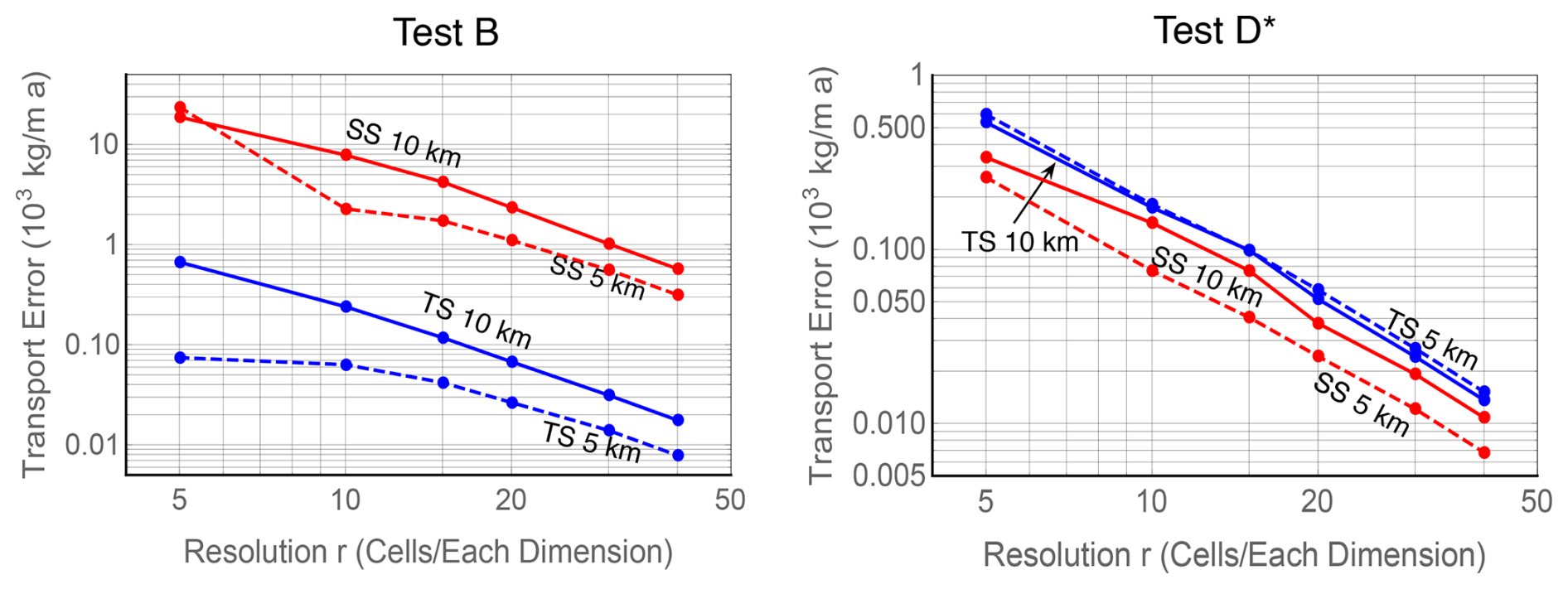
Figure 3 Convergence of ice transport in tests B and D^∗ with mesh refinement. Transformed Stokes (TS) plots are in blue, and standard Stokes plots (SS) are in red.

Figure 4 The u-velocity profile at location x=L as a function of height from the bed.

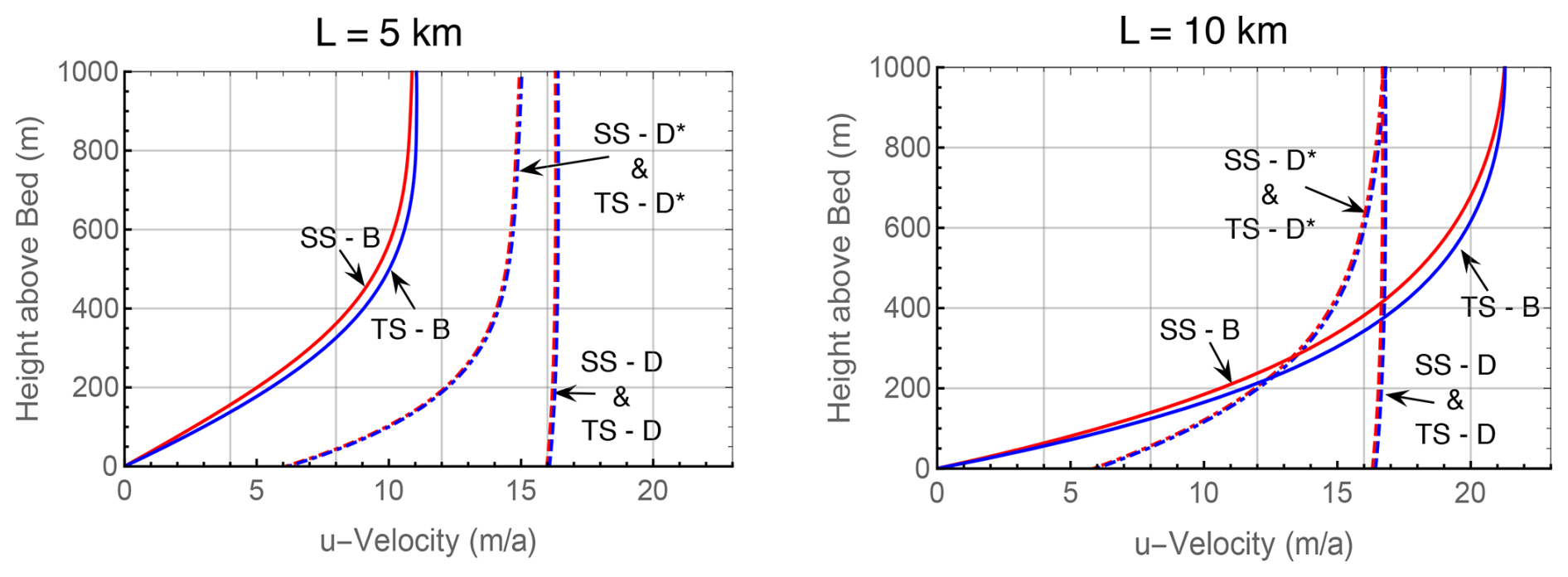
Figure 3 evaluates the convergence of the two Stokes formulations as a function of mesh resolution r, where r is the number of quadrilaterals in either direction. The models converge to the same value of the transport, obtained by Richardson extrapolation, and convergence is second order as expected from the use of linear elements. Interestingly, in Test B the transformed Stokes model is considerably more accurate at all resolutions than the standard model. As a result, the standard Stokes calculations are not fully converged even at the 40×40 resolution. Figure 4 shows the vertical profiles of the horizontal velocity u at outflow, x=L. Results from the no-slip Test B problem and the two frictional sliding problems, tests D and D^∗, are plotted. The Test D profile from the ISMIP-HOM benchmark is almost vertically constant, indicating that the value for basal friction that was originally chosen is too small. This motivated the change of Test D to Test D^∗ in Appendix C, with larger basal friction.

Figure 5 Upper surface u velocity, u(x,z_s) – Test B, no-slip boundary conditions.

Figure 6 Upper surface u velocity, u(x,z_s) – Test D^∗, modified frictional sliding.

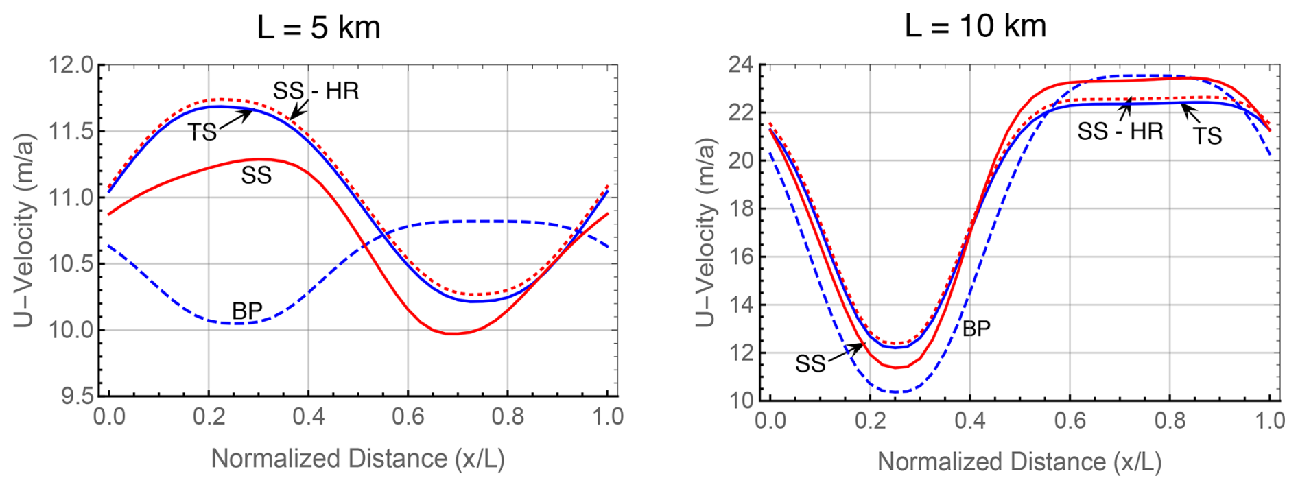
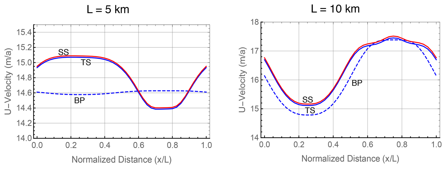
Figures 5 and 6 show the u velocity at the ice sheet upper surface for tests B and D^∗. This is the benchmark used in ISMIP-HOM to compare different ice sheet models. Four cases are compared: the standard Stokes model (SS), the transformed Stokes model (TS), the Blatter–Pattyn (BP) model, and for reference a very high resolution full Stokes Test B calculation “oga1” (SS-HR) from the ISMIP-HOM paper and also Gagliardini and Zwinger (2008). The TS and the SS-HR plots lie on top of one another (they have been offset slightly for clarity), indicating that the TS model is already fully converged. As before, the SS model is not yet converged in Test B, particularly at L=5 km. As in the ISMIP-HOM study, the Blatter–Pattyn calculation (BP) shows large deviations from the Stokes results, especially so at L=5 km, where the surface velocity is entirely out of phase with the Stokes results. Figure 6 shows that results for the SS and TS models essentially coincide in Test D^∗ (the SS plot has been slightly offset upward for clarity). As expected, Blatter–Pattyn results show noticeable error at L=10 km and very large error at L=5 km. Pressure results are not presented since they have no physical significance. However, it may be noted that pressures on the P1–E0 mesh are particularly smooth and well behaved.

6 Applications of the transformed Stokes model

6.1 Adaptive switching between Stokes and Blatter–Pattyn models

A way of reducing the cost of a full Stokes calculation is to use it adaptively together with a cheaper approximate model. That is, one may use the cheaper model in those parts of a problem where it is accurate and the more expensive full Stokes model where the approximate model loses accuracy. An example of such an adaptive approach is the tiling method by Seroussi et al. (2012). However, such methods have drawbacks such as the need to incorporate two or more presumably quite different models into a single model together with a transition zone to couple the disparate models.

On the other hand, the use of the transformed Stokes model is particularly simple in such an adaptive role because it may be locally switched between the Stokes and Blatter–Pattyn cases by switching the parameter $\mathit{\xi }\in \left\{\mathrm{0},\mathrm{1}\right\}$ on and off. Either the standard or the extended Blatter–Pattyn models may be used. Use of the standard Blatter–Pattyn approximation ($\mathit{\xi },\widehat{\mathit{\xi }}=\mathrm{0})$ would be somewhat cheaper, but it would require more complicated programming; i.e., it would need coupling to the Stokes model with p=0 and $\mathit{w}=\mathit{w}\left(\mathit{u},\mathit{v}\right)$ at the interface between models. Use of the extended Blatter–Pattyn approximation ($\mathit{\xi }=\mathrm{0},\widehat{\mathit{\xi }}=\mathrm{1})$ would be much simpler since then both the Stokes and Blatter–Pattyn parts of the code will have the same number of degrees of freedom. However, as explained in Sect. 4.3, the extended Blatter–Pattyn model requires a mesh satisfying the solvability condition, such as the P1–E0 mesh. Although a little more expensive than standard Blatter–Pattyn, the extended Blatter–Pattyn model is still much cheaper than the full Stokes model. For example, the extended Blatter–Pattyn calculation of Test B at a 40×40 resolution, as in Figs. 5 and 6, is some 4.3 times cheaper than the corresponding transformed Stokes calculation.

To demonstrate adaptive switching with a transformed Stokes model, we introduce a new problem, Test O, described in Appendix C and illustrated in Fig. C1. This consists of an inclined ice slab whose movement is obstructed by a thin obstacle protruding 20 % of the ice depth up from the bed. No-slip boundary conditions are applied along the bed and the obstacle. Because of the localized nature of the obstacle, the condition for the validity of the Blatter–Pattyn approximation, namely (37), must fail near the obstacle, and therefore the full Stokes model is needed for good accuracy, at least locally.

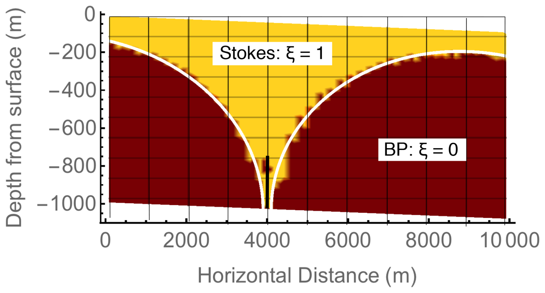
Figure 7 Mask function (white curve, z=F_M(x)) to indicate where the Stokes and BP models are activated in the 20 % obstacle test problem. The dark brown region delineates the region where $\left|\partial w/\partial x\right|\le \mathrm{0.1}\left|\partial u/\partial z\right|$ from a Blatter–Pattyn calculation.

To implement the method, we first use a Blatter–Pattyn calculation to determine regions where $\left|\partial w/\partial x\right|\le \mathrm{0.1}\left|\partial u/\partial z\right|$, approximately localizing where the Blatter–Pattyn approximation is valid. This determines a mask function z=F_M(x), illustrated in Fig. 7 by the white curve, specifying where the two models must be used. Defining the centroid of a triangular element by (x_C,z_C), the code makes a selection in each element:

$$\begin{array}{l}{z}_C\le F_M\left(x_C\right)\Rightarrow \text{Set }\mathit{\xi }=\mathrm{0},\text{i.e.,\hspace{0.17em} the\hspace{0.17em} Blatter–Pattyn\hspace{0.17em} region,}\\ z_C>F_M\left(x_C\right)\Rightarrow \text{Set }\mathit{\xi }=\mathrm{1},\text{i.e.,\hspace{0.17em} the\hspace{0.17em} Stokes\hspace{0.17em} region.}\end{array}$$

The Stokes region occupies the upper part of the domain in Fig. 7 and includes the obstacle, while the Blatter–Pattyn region occupies much of the bottom part of the domain. A transition zone, e.g., $\mathrm{0}\le \mathit{\xi }\left(x,z\right)\le \mathrm{1}$, could be implemented, but this was not done in the present case.

Results from the adaptive-hybrid calculation are shown in Fig. 8, showing curves of the horizontal velocity u at seven different vertical locations specified as a percentage of the distance between top and bottom, with σ=100 % at the top surface. The top-right panel shows the results for the adaptive-hybrid calculation (AH), and the top-left panel and bottom panel show results for the Stokes (TS) and Blatter–Pattyn (BP) calculations, respectively. All calculations use the 40×40 mesh resolution. The adaptive-hybrid results are very similar to the full Stokes results, reproducing most features of the velocity profiles, including the velocity bump at the top surface, indicating that even the top surface feels the presence of the obstacle. The Blatter–Pattyn results are much less accurate, completely missing the details of the flow near the obstacle. The calculated RMS error relative to the Stokes results in the Blatter–Pattyn case is 0.493 and 0.440 m a⁻¹ in the adaptive-hybrid case. It is larger in the Blatter–Pattyn case, as expected, but the difference is less than expected from the visual differences in Fig. 8. Nonetheless, the adaptive-hybrid method is successful even if judged by the Fig. 8 results alone. However, the present calculations are proof of concept only and not representative of practical computational methods, so computational cost comparisons would not be meaningful.

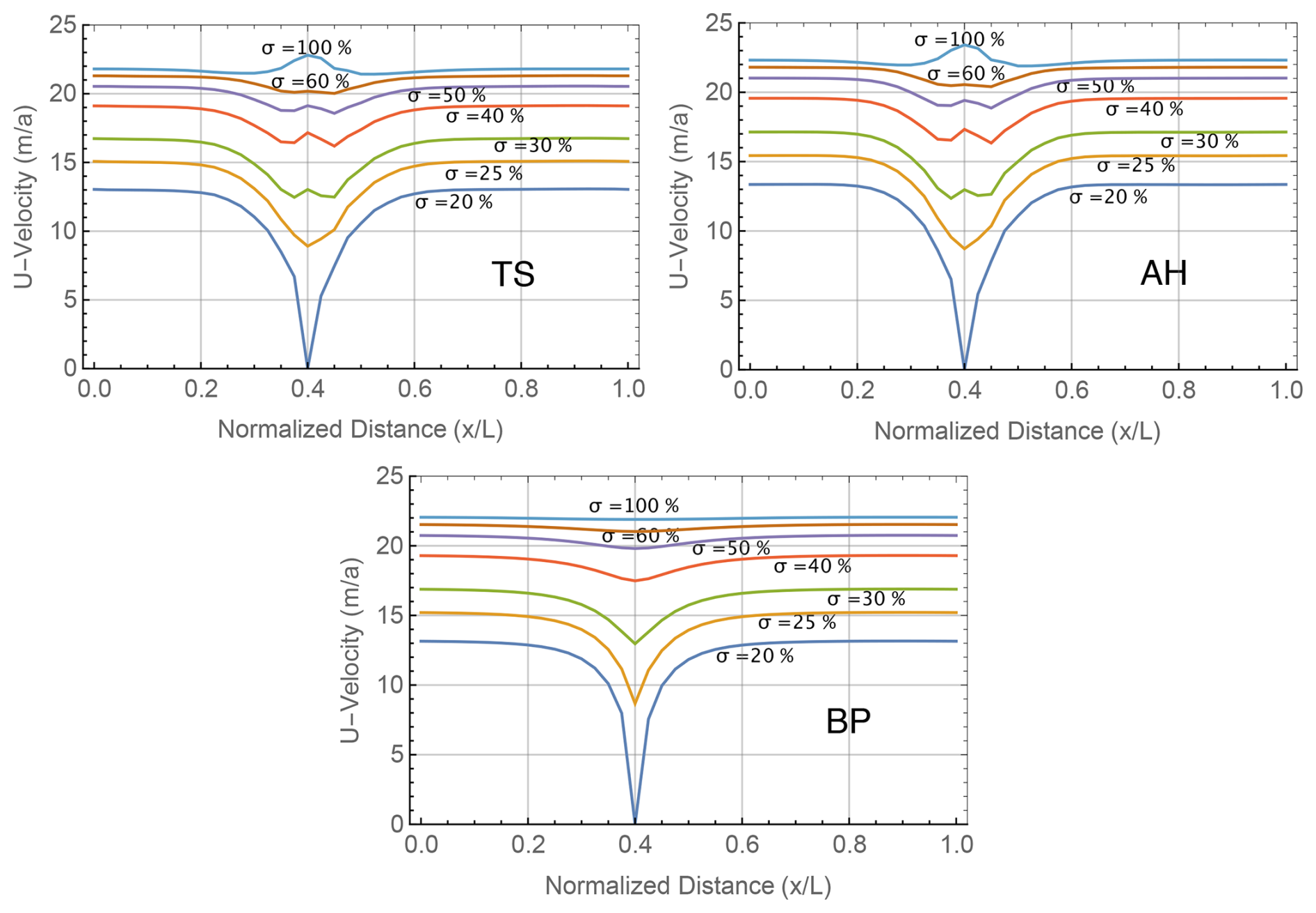
Figure 8 Horizontal velocity for the transformed Stokes (TS), the adaptive-hybrid (AH), and the Blatter–Pattyn (BP) models in Test O.

6.2 Two new Stokes approximations

As shown in Sect. 3.4, simply setting w=0 in the second invariant ${\stackrel{\mathrm{̃}}{\dot{\mathit{\epsilon }}}}^{\mathrm{2}}$ in the transformed functional $\stackrel{\mathrm{̃}}{A}$ results in the standard Blatter–Pattyn approximation. This suggests that approximating rather than neglecting the vertical velocity w in the functional would create better approximations. We will look at two such methods, although others may be possible. The first method, called the Herterich approximation, may be understood as the Picard iteration of the transformed functional (32), where the vertical velocity, obtained from the solution of the continuity equation, is a lagged value from the previous iteration. Two ways of implementing this method are described. The second method, to be called the dual-mesh approximation, approximates the vertical velocity by discretizing the continuity equation on a coarser mesh. Since vertical velocity is obtained from inverting the continuity equation, this has the effect of approximating the vertical velocity and reducing the number of pressure and vertical velocity variables while preserving the structure of the Stokes model. The degree of approximation is determined by the amount of coarsening of the continuity mesh.

6.2.1 The Herterich approximation

Noting that $\stackrel{\mathrm{̃}}{P}=\mathrm{0}$ in the Blatter–Pattyn approximation, we drop the term involving pressure from the transformed functional (32) in the 2D case to obtain a new pressure-free functional,

$$\begin{array}{}\text{(61)}& \begin{array}{rl}{\stackrel{\mathrm{̃}}{A}}_{\mathrm{PS}\mathrm{1}}\left[u\right]& =\underset{V}{\int }dV\left[{\displaystyle \frac{\mathrm{4}n}{n+\mathrm{1}}}{\mathit{\eta }}_{\mathrm{0}}{\left({\stackrel{\mathrm{̃}}{\dot{\mathit{\epsilon }}}}^{\mathrm{2}}\right)}^{\left(\mathrm{1}+n\right)/\mathrm{2}n}+\mathit{\rho }gu{\displaystyle \frac{\partial z_s}{\partial x}}\right]\\ & +{\displaystyle \frac{\mathrm{1}}{\mathrm{2}}}\underset{S_{B\mathrm{2}}}{\int }dS\mathit{\beta }\left(x\right)\left(u^{\mathrm{2}}+\mathit{\zeta }{\left(u{n}_x/n_z\right)}^{\mathrm{2}}\right),\end{array}\end{array}$$

where

$$\begin{array}{}\text{(62)}& {\stackrel{\mathrm{̃}}{\dot{\mathit{\epsilon }}}}^{\mathrm{2}}={\left({\displaystyle \frac{\partial u}{\partial x}}\right)}^{\mathrm{2}}+{\displaystyle \frac{\mathrm{1}}{\mathrm{4}}}{\left({\displaystyle \frac{\partial u}{\partial z}}+{\displaystyle \frac{\partial w}{\partial x}}\right)}^{\mathrm{2}}\end{array}$$

is the 2D version of the transformed second invariant, (27). Incompressibility is incorporated separately by the use of a second functional,

$$\begin{array}{}\text{(63)}& {\stackrel{\mathrm{̃}}{A}}_{\mathrm{PS}\mathrm{2}}\left[p\right]=\underset{V}{\int }dVp\left({\displaystyle \frac{\partial u}{\partial x}}+{\displaystyle \frac{\partial w}{\partial z}}\right).\end{array}$$

Both functionals make use of direct substitution for boundary conditions, as in (15) and (32). Note that functional (61) involves both velocity components u,w, but the variation is to be taken only with respect to u. Similarly, functional (63) involves $u,w,p$, but the variation is taken only with respect to p. Here we are effectively viewing the pressure p as a “test function” in the finite element sense. This gives some additional flexibility to create elements that satisfy the solvability condition (58). For example, in a triangulation some pressures may be assigned to every two triangles, as in a P1–E0 mesh, while others may be assigned to a single triangle so as to achieve an equal number of pressure and vertical velocity variables.

The variation of ${\stackrel{\mathrm{̃}}{A}}_{\mathrm{PS}\mathrm{1}}\left[u\right]$ with respect to u results in a set of n_u discrete Euler–Lagrange equations corresponding to the u-momentum equation,

$$\begin{array}{}\text{(64)}& {\widehat{\mathit{R}}}_U\left(\mathit{u},\mathit{w}\right)={\displaystyle \frac{\partial {\stackrel{\mathrm{̃}}{A}}_{\mathrm{PS}\mathrm{1}}\left(\mathit{u},\mathit{w}\right)}{\partial \mathit{u}}}=M_U\left(\mathit{u},\mathit{w}\right)+{\mathit{f}}_U=\mathrm{0}.\end{array}$$

When w is set to zero, this is just the Blatter–Pattyn model, (49). The discrete variation of ${\stackrel{\mathrm{̃}}{A}}_{\mathrm{PS}\mathrm{2}}\left[\mathit{p}\right]$ with respect to p results in the n_p equations of the discrete continuity equation (55),

$$\begin{array}{}\text{(65)}& {\widehat{\mathit{R}}}_P\left(\mathit{u},\mathit{w}\right)={\displaystyle \frac{\partial {\stackrel{\mathrm{̃}}{A}}_{\mathrm{PS}\mathrm{2}}\left(\mathit{u},\mathit{w},\mathit{p}\right)}{\partial \mathit{p}}}={\mathbf{M}}_{\mathrm{UP}}^T\mathit{u}+{\mathbf{M}}_{\mathrm{WP}}^T\mathit{w}=\mathrm{0}.\end{array}$$

These two systems are combined to form the discrete equations of the Herterich approximation,

$$\begin{array}{}\text{(66)}& \widehat{\mathit{R}}\left(\mathit{u},\mathit{w}\right)={\left[{\widehat{\mathit{R}}}_U\left(\mathit{u},\mathit{w}\right),{\widehat{\mathit{R}}}_P\left(\mathit{u},\mathit{w}\right)\right]}^T=\mathrm{0}.\end{array}$$

This is a system of n_u+n_p equations to determine the n_u+n_w discrete variables u,w, implying that (66) is only a viable system for u,w on meshes satisfying the solvability condition, n_p=n_w. Just as in the standard Blatter–Pattyn approximation in Sect. 3.4.1, the vertical momentum equation is missing, but instead of neglecting w here the vertical velocity is obtained consistently from the continuity equation.

The continuum form of the discrete Euler–Lagrange system (64) and (65) is given by

$$\begin{array}{}\text{(67)}& \begin{array}{rl}{\displaystyle \frac{\partial }{\partial x}}\left(\mathrm{4}\stackrel{\mathrm{̃}}{\mathit{\mu }}{\displaystyle \frac{\partial u}{\partial x}}\right)& +{\displaystyle \frac{\partial }{\partial z}}\left(\stackrel{\mathrm{̃}}{\mathit{\mu }}\left({\displaystyle \frac{\partial u}{\partial z}}+{\displaystyle \frac{\partial w}{\partial x}}\right)\right)-\mathit{\rho }g{\displaystyle \frac{\partial z_s}{\partial x}}=\mathrm{0},\\ & {\displaystyle \frac{\partial u}{\partial x}}+{\displaystyle \frac{\partial w}{\partial z}}=\mathrm{0},\end{array}\end{array}$$

together with the boundary conditions,

$$\begin{array}{}\text{(68)}& \begin{array}{rl}& \mathrm{4}\stackrel{\mathrm{̃}}{\mathit{\mu }}{\displaystyle \frac{\partial u}{\partial x}}{n}_x+\stackrel{\mathrm{̃}}{\mathit{\mu }}\left({\displaystyle \frac{\partial u}{\partial z}}+{\displaystyle \frac{\partial w}{\partial x}}\right)n_z=\mathrm{0}\text{on}{S}_S,\\ & u=w=\mathrm{0}\text{on}{S}_{B\mathrm{1}},\\ & \mathrm{4}\stackrel{\mathrm{̃}}{\mathit{\mu }}{\displaystyle \frac{\partial u}{\partial x}}{n}_x+\stackrel{\mathrm{̃}}{\mathit{\mu }}\left({\displaystyle \frac{\partial u}{\partial z}}+{\displaystyle \frac{\partial w}{\partial x}}\right)n_z+\mathit{\beta }\left(x\right)\left(u+\mathit{\zeta }u{\left(n_x/n_z\right)}^{\mathrm{2}}\right)=\mathrm{0},\\ & \left.w=-u{n}_x/n_z,\right\}\text{on}{S}_{B\mathrm{2}},\end{array}\end{array}$$

where the viscosity is $\stackrel{\mathrm{̃}}{\mathit{\mu }}={\mathit{\eta }}_{\mathrm{0}}{\left({\stackrel{\mathrm{̃}}{\dot{\mathit{\epsilon }}}}^{\mathrm{2}}\right)}^{(\mathrm{1}-n)/\mathrm{2}n}$ as in (26). Remarkably, these are the same equations used by Herterich (1987) in a model to study the transition zone between an ice sheet and an ice shelf¹. As a result, this approximation is named the Herterich model. The Herterich model predates the widely used Blatter–Pattyn model by some 8 years, but, in contrast to Blatter–Pattyn, it has fallen into obscurity.

There are two algorithms for solving the Herterich system (66), as follows:

1. Newton/Picard iteration version.

   If we lag the vertical velocity, i.e., ${\mathit{w}}^{K+\mathrm{1}}={\mathit{w}}^K\Rightarrow \mathrm{\Delta }\mathit{w}=\mathrm{0}$ in the first equation of (70), we obtain a Picard iteration algorithm, as follows:

   $$\begin{array}{}\text{(69)}& \begin{array}{rl}& \text{Starting from}K=\mathrm{0},\text{choose an initial guess},\\ & {\mathit{u}}^{\mathrm{0}}\ne \mathrm{0},\mathit{w}\left({\mathit{u}}^{\mathrm{0}}\right),\\ & \text{solve\hspace{0.17em} \hspace{0.17em} }{\mathbf{M}}_{\mathrm{UU}}\left({\mathit{u}}^K,{\mathit{w}}^K\right)\mathrm{\Delta }\mathit{u}+{\widehat{\mathit{R}}}_U\left({\mathit{u}}^K,{\mathit{w}}^K\right)=\mathrm{0},\\ & {\mathit{u}}^{K+\mathrm{1}}={\mathit{u}}^K+\mathrm{\Delta }\mathit{u},{\mathit{w}}^{K+\mathrm{1}}=\mathit{w}\left({\mathit{u}}^{K+\mathrm{1}}\right)\\ & =-{\mathbf{M}}_{\mathrm{WP}}^{-T}{\mathbf{M}}_{\mathrm{UP}}^T{\mathit{u}}^{K+\mathrm{1}},\\ & K=K+\mathrm{1},\text{and repeat until convergence}.\end{array}\end{array}$$

   Each step of the iteration is inexpensive since it is equivalent to a step of the standard Blatter–Pattyn model, (35). However, Picard iterations typically converge only linearly.

2. Quasi-variational, Newton iteration version.

   To obtain second-order convergence we treat (66) as a single multidimensional nonlinear system and solve it using the Newton–Raphson iteration, as follows:

   $$\begin{array}{}\text{(70)}& \begin{array}{rl}& {\mathbf{M}}_{\mathrm{UU}}\left({\mathit{u}}^K,{\mathit{w}}^K\right)\mathrm{\Delta }\mathit{u}+{\mathbf{M}}_{\mathrm{UW}}\left({\mathit{u}}^K,{\mathit{w}}^K\right)\mathrm{\Delta }\mathit{w}+{\widehat{\mathit{R}}}_U\left({\mathit{u}}^K,{\mathit{w}}^K\right)\\ & =\mathrm{0},\\ & {\mathbf{M}}_{\mathrm{UP}}^T{\mathit{u}}^{K+\mathrm{1}}+{\mathbf{M}}_{\mathrm{WP}}^T{\mathit{w}}^{K+\mathrm{1}}=\mathrm{0},\end{array}\end{array}$$

   where K is the iteration index, Δu and Δw were defined previously, and M_UU(u,w) and M_UW(u,w) are the same matrices as appear in (48). Convergence is rapid (quadratic) once in the basin of attraction, but each step is more expensive than in the Picard iteration version. Both versions depend on an invertible continuity equation to obtain w=w(u). However, good approximations of the vertical velocity w(u) may already be available in existing codes – for instance, in MALI (Hoffman et al., 2018), a code based on the Blatter–Pattyn approximation, to obtain the vertical velocity w for the advection of ice temperature (Mauro Perego, personal communication, 2023).

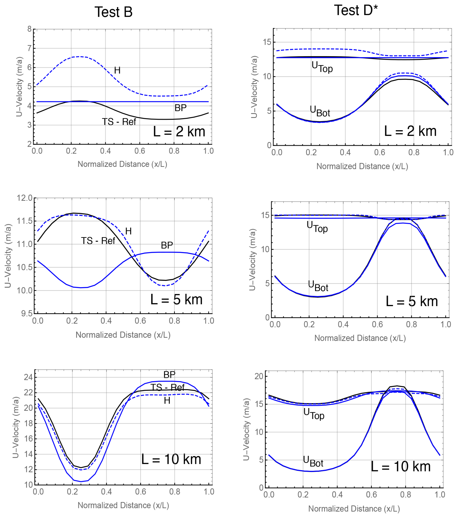
Figure 9 Comparing approximations. Test B, upper surface u velocity, and Test D^∗, upper and lower surface u velocity. TS-Ref: transformed Stokes; BP: Blatter–Pattyn; H: Herterich. Resolution: 24×24.

Both Herterich algorithms converge to the same result. It remains to be seen which version is preferable in practice. Figure 9 compares the Herterich (H) and the Blatter–Pattyn (BP) approximations to a reference exact transformed Stokes solution (TS-Ref) for Test B results on the left and Test D^∗ results on the right at three problem aspect ratios in the range where small aspect ratio approximation begins to fail, $\mathit{\epsilon }=H_{\mathrm{0}}/L=\mathrm{0.1},\mathrm{0.2},\mathrm{0.5}$, where H₀=1000 m is the nominal ice thickness and L is the domain length. The Herterich approximation might be expected to be more accurate than the BP approximation since it retains more terms from the transformed Stokes model equations, but this is not borne out in Fig. 9. The Herterich approximation is indeed more accurate in Test B at $L=\mathrm{5},\mathrm{10}$ km. This is confirmed by the RMS u-error results in Fig. 12, where the Herterich model is 2 to 3 times more accurate than BP. However, the opposite is the case at L=2 km in both tests B and D^∗, although the results in Test B may be deceptive because only the upper surface velocity is displayed (lower surface velocity is zero), and this expands the scale accentuating differences between the three cases. Test D^∗ results are closely clustered except in the L=2 km case, where, surprisingly, the Herterich approximation is the least accurate. These results suggest that the Herterich approximation may need to be evaluated further.

6.2.2 A dual-mesh transformed Stokes approximation

In the Herterich approximation we approximated the vertical velocity directly in the second invariant as it appeared in the variational functional. Here we approximate w indirectly by instead approximating the continuity equation that is then used to determine the vertical velocity. That is, the continuity equation is discretized on a mesh coarser than the one used for the momentum equations. The vertical velocity on the coarser mesh is then interpolated to appropriate locations on the finer mesh. This reduces the number of unknown variables in the problem, making it cheaper to solve but hopefully without serious loss of accuracy. As described in Appendix C, our test problem meshes are logically rectangular, i.e., divided into n cells horizontally and m cells vertically. The coarse mesh is constructed by dividing the fine mesh into s equal segments in each direction. This assumes that the integers n and m are each divisible by s, so that there are $nm/s^{\mathrm{2}}$ coarse cells in total with each coarse cell containing s² fine cells. The primary mesh (i.e., the fine mesh) is chosen to have $n=m=\mathrm{24}$, i.e., a reference 24×24 fine mesh, so as to maximize the number of different coarse meshes available. Coarse meshes are constructed using $s=\mathrm{2},\mathrm{3},\mathrm{4},\mathrm{6}$, and this results in fine-mesh and coarse-mesh combinations labeled by $\mathrm{24}\times \mathrm{12},\mathrm{24}\times \mathrm{8},\mathrm{24}\times \mathrm{6},\mathrm{24}\times \mathrm{4}$, respectively. Similar to a P1–E0 fine mesh, coarse-mesh vertical velocities w are located at vertices and pressures at vertical edges. Figure 10 illustrates the case of a single coarse cell and four fine quadrilateral cells for a mesh fragment with $n=m=\mathrm{2}$ and s=1. In Test B problems with direct substitution for basal boundary conditions there will be nm u variables and $nm/s^{\mathrm{2}}$ w and p variables each, for a total of $nm\left(\mathrm{1}+\mathrm{2}/s^{\mathrm{2}}\right)$ unknown variables, considerably fewer than the 3 nm variables in the full-resolution mesh. The coarse-mesh terms in the functional that are affected, $\stackrel{\mathrm{̃}}{P}\left(\partial u/\partial x+\partial w/\partial z\right)$ and $\partial w/\partial x$, are computed by interpolating coarse-mesh variables to the fine mesh. We consider two versions of the approximation depending on how the coarse-mesh terms are interpolated to the fine mesh.

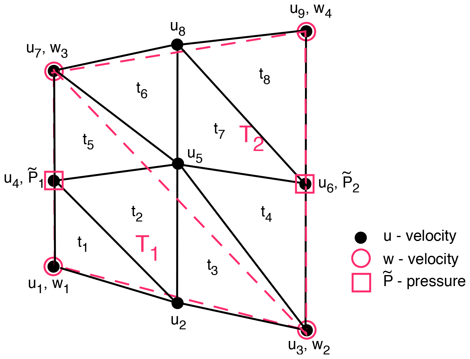
Figure 10 A sample of a coarse/fine P1–E0 mesh for the dual-mesh approximation. Resolution: $n=m=\mathrm{2},s=\mathrm{1}$. Coarse mesh is in red; fine mesh is in black.

1. Approximation A, bilinear interpolation.

   Referring to Fig. 10, the four velocities at the vertices of the coarse-mesh quadrilateral, i.e., $u_{\mathrm{1}},u_{\mathrm{3}},u_{\mathrm{7}},u_{\mathrm{9}}$ and $w_{\mathrm{1}},w_{\mathrm{2}},w_{\mathrm{3}},w_{\mathrm{4}}$, are used to obtain u,w at the remaining five vertices of the fine mesh by means of bilinear interpolation. Thus, the five velocities $u_{\mathrm{2}},u_{\mathrm{4}},u_{\mathrm{5}},u_{\mathrm{6}},u_{\mathrm{8}}$ are obtained in terms of vertex velocities $u_{\mathrm{1}},u_{\mathrm{3}},u_{\mathrm{7}},u_{\mathrm{9}}$, and similarly for the w velocities. The resulting complete set of fine-mesh variables is used calculate the divergence $D=\left(\partial u/\partial x+\partial w/\partial z\right)$ and the quantity $\partial w/\partial x$ in each of the eight triangular elements $t_{\mathrm{1}},t_{\mathrm{2}},\mathrm{\dots },t_{\mathrm{8}}$ of the fine mesh. Coarse-mesh pressures ${\stackrel{\mathrm{̃}}{P}}_{\mathrm{1}},{\stackrel{\mathrm{̃}}{P}}_{\mathrm{2}}$ are associated with the coarse-mesh triangles T₁,T₂. The products ${\stackrel{\mathrm{̃}}{P}}_{\mathrm{1}}D$ in elements $t_{\mathrm{1}},t_{\mathrm{2}},t_{\mathrm{3}},t_{\mathrm{5}}$ and ${\stackrel{\mathrm{̃}}{P}}_{\mathrm{2}}D$ in elements $t_{\mathrm{4}},t_{\mathrm{6}},t_{\mathrm{7}},t_{\mathrm{8}}$ are then accumulated over the entire mesh to obtain the quantity $\stackrel{\mathrm{̃}}{P}\left(\partial u/\partial x+\partial w/\partial z\right)$ for use in the transformed functional $\stackrel{\mathrm{̃}}{A}$. Similarly, the quantity $\partial w/\partial x$ is computed in the fine-mesh elements from coarse-mesh variables for use in the second invariant ${\stackrel{\mathrm{̃}}{\dot{\mathit{\epsilon }}}}^{\mathrm{2}}$.

2. Approximation B, linear interpolation.

   In this version, the three velocities at the vertices of the two coarse-mesh triangles T₁ and T₂, i.e., $u_{\mathrm{1}},u_{\mathrm{3}},u_{\mathrm{7}}$ and $w_{\mathrm{1}},w_{\mathrm{2}},w_{\mathrm{3}}$ in T₁, and $u_{\mathrm{7}},u_{\mathrm{3}},u_{\mathrm{9}}$ and $w_{\mathrm{3}},w_{\mathrm{2}},w_{\mathrm{4}}$ in T₂, approximate the divergence $D=\left(\partial u/\partial x+\partial w/\partial z\right)$ and $\partial w/\partial x$ as constant values in the two coarse triangles. The constant values ${\stackrel{\mathrm{̃}}{P}}_{\mathrm{1}}D$, ${\stackrel{\mathrm{̃}}{P}}_{\mathrm{2}}D$ are then accumulated over the entire mesh. The constant value $\partial w/\partial x$ in each coarse triangle is then distributed to each of the eight fine-mesh elements $t_{\mathrm{1}},t_{\mathrm{2}},\mathrm{\dots },t_{\mathrm{8}}$, depending on whether the centroid of the fine triangular element is in T₁ or T₂. As in the previous case, this is then used in the second invariant ${\stackrel{\mathrm{̃}}{\dot{\mathit{\epsilon }}}}^{\mathrm{2}}$ in the transformed functional $\stackrel{\mathrm{̃}}{A}$.

While the number and type of unknown variables is the same in the two versions, they differ considerably in accuracy as seen in Figs. 11 and 12. Figure 11 compares the upper surface u velocity in approximations A and B, for the five mesh combinations, to the reference 24×24 fine-mesh transformed Stokes (TS) calculation. The corresponding Blatter–Pattyn result is shown in Fig. 9. Figure 12 summarizes and compares the overall accuracy of all approximations by means of the RMS u-error relative to the TS calculation. As might be expected, the accuracy of Approximation A is better than Approximation B, particularly in the case L=10 km. Both dual-mesh versions are more accurate than the BP and H approximations, except for the lowest 24×4 resolution of Approximation B. However, it is surprising that the SS calculation is the least accurate, but this is because SS is not yet fully converged at this resolution (see Fig. 5).

A comparison of computational time relative to the TS calculation is presented in Fig. 12 for the 24×24 resolution case. The cost of the BP approximation is substantially lower than the cost of full Stokes, while the cost of the Herterich approximation is only slightly higher than BP. This comparison is only qualitative because the present calculations are not representative of the computer hardware or the methods used in practical ice sheet modeling. Present calculations are proof of concept only, made on a personal computer using the program Mathematica, a slow interpreted language. As a result the cost comparisons are inaccurate and possibly misleading. No effort was made to optimize the calculations or to take advantage of parallelization. Thus, for example, the cost of dual-mesh approximations A and B is greatly affected by the cost of the associated interpolations, making them more costly than even the unapproximated calculations, TS and SS. However, the interpolations are highly parallelizable and would contribute little to the cost in practical computations.

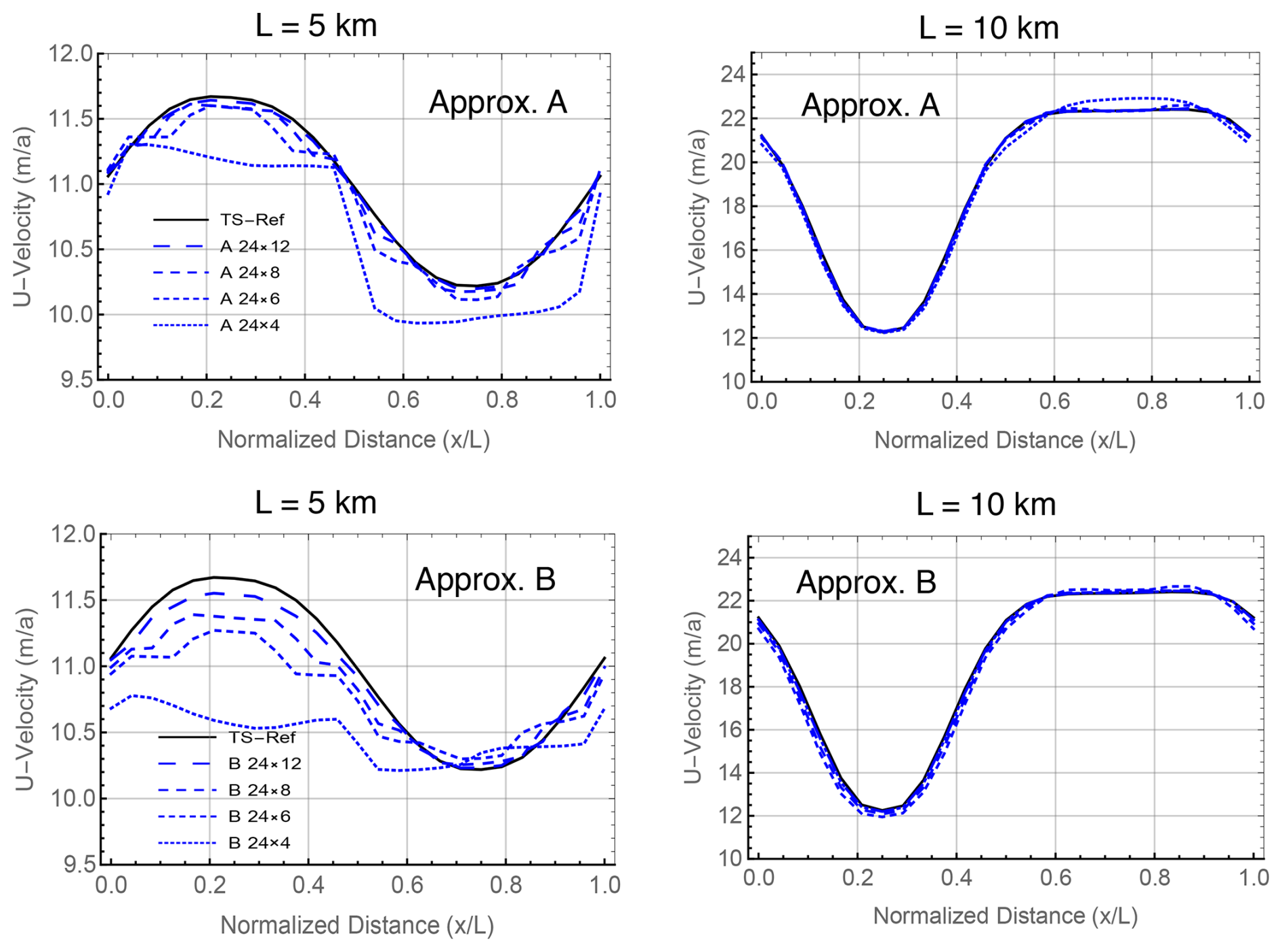
Figure 11 Comparing approximations A and B. Test B. Upper surface u velocity. TS-Ref: reference Stokes ($r\times r=\mathrm{24}\times \mathrm{24}$); fine/coarse resolutions ($rxR=\mathrm{24}\times \mathrm{12}$, 8, 6, 4).

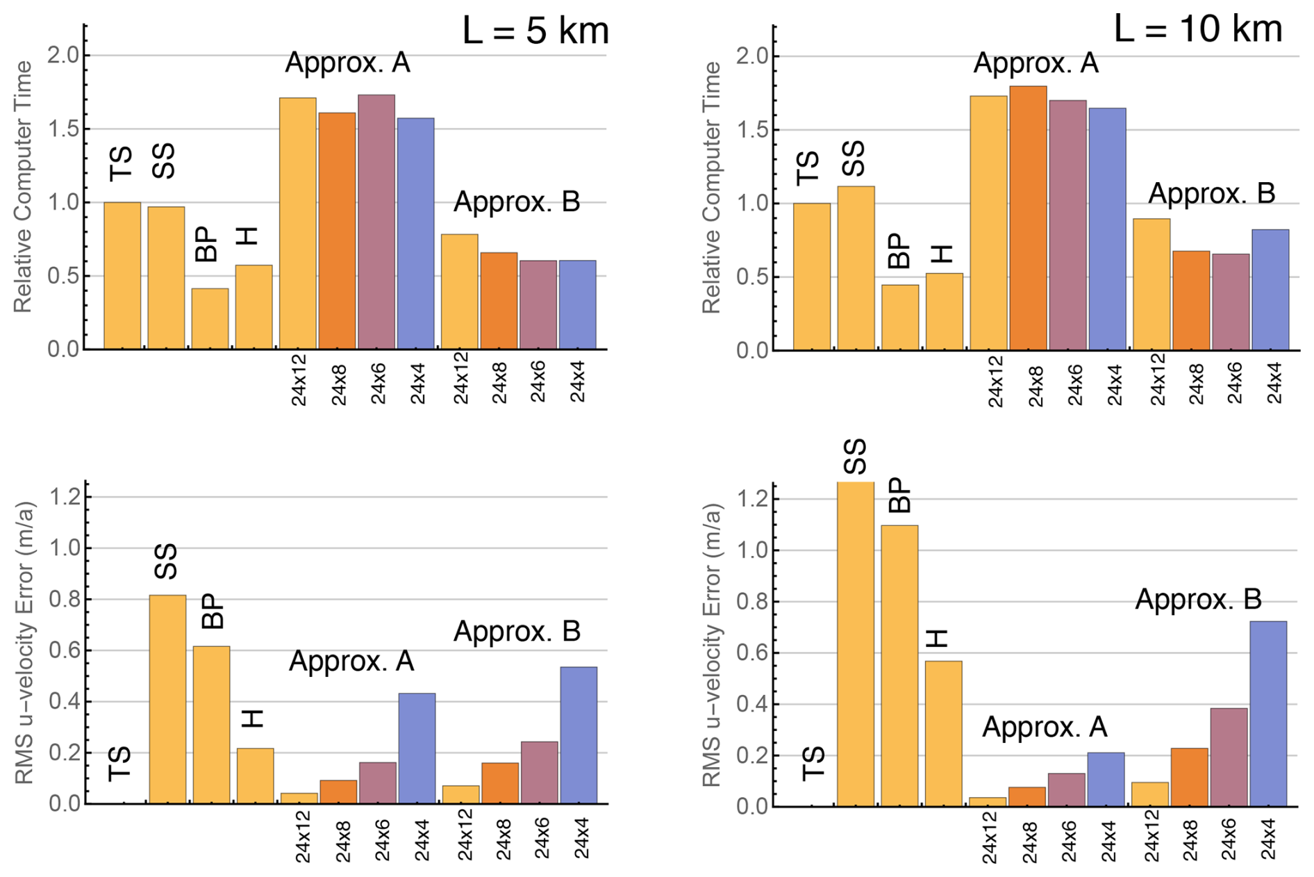
Figure 12 Comparing the Test B computer time and RMS u-error results relative to a TS calculation for approximations BP, H, A, and B and the SS Stokes model. TS, SS, BP, H: resolution ($rxr=\mathrm{24}\times \mathrm{24}$); approximations A and B: ($rxR=\mathrm{24}\times \mathrm{12}$, 8, 6, 4).

7 Second-order discretizations

So far we have used first-order elements, primarily P1–E0. However, in current practice Stokes models are often based on second-order elements such as the popular Taylor–Hood P2–P1 element (e.g., Leng et al., 2012; Gagliardini et al., 2013). In 2D the P2–P1 element, illustrated in Fig. 13a, has velocities on element vertices and edge midpoints and pressures on element vertices, resulting in quadratic velocity and linear pressure distributions. This element satisfies the inf-sup stability condition (e.g., Elman et al., 2014) but does not satisfy the solvability condition (58) since n_w≫n_p. For example, in the present Test B calculations we have n_w=4n m and $n_p=n\left(m+\mathrm{1}\right)$.

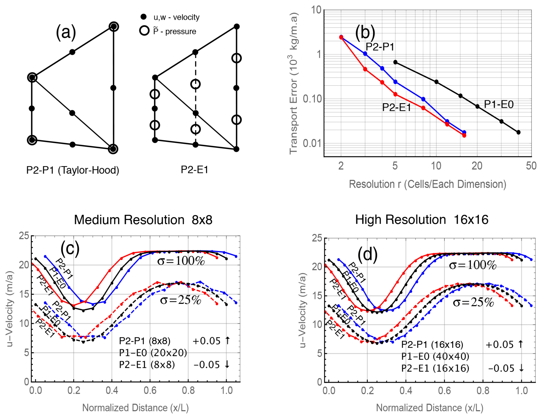
Figure 13 Comparing second-order discretizations based on the P2–P1 and P2–E1 elements from panel (a) to first-order discretizations using the P1–E0 element in Test B calculations with L=10 km. Only transformed Stokes calculations are compared; standard Stokes results behave similarly. Panel (b) compares the convergence and accuracy of various schemes with increasing resolution, while panels (c) and (d) compare horizontal velocities at medium and maximum resolutions.

Stokes models work well with a Taylor–Hood mesh as shown in Fig. 13, where both the P2–P1 and P1–E0 models converge to a common solution. Recall that the P2–P1 mesh does not work with the extended Blatter–Pattyn approximation, a model that requires the solvability condition. However, it is possible to construct a second-order element consistent with an invertible continuity equation. This is the P2–E1 element, as illustrated in Fig. 13a, which is second order for velocities and linear for pressure, just like the P2–P1 element, but the pressure is edge-based rather than vertex-based. Pressures are located midway between velocities along vertical lines, as illustrated in Fig. 13a. As explained in Appendix A, this mesh must be constructed using vertical columns of quadrilaterals. Since pressures are vertically collinear with velocities, as in the P1–E0 element, the analysis in Appendix A confirms that this element satisfies the solvability condition (58). A 3D analog exists, as explained in Appendix A.

Figure 13b shows the error in ice transport as a function of mesh refinement for the second-order P2–P1 and P2–E1 meshes in transformed Stokes Test B calculations, together with similar results for the first-order P1–E0 mesh from Fig. 3 for comparison. Note that both second-order models show approximately the same error at resolution r=16 as the first-order P1–E0 model at resolution r=40, and the same for coarser resolutions such as r=8 and r=20, respectively. However, at a comparable resolution or accuracy the second-order calculations are considerably more expensive than the first-order calculations.

Figures 13c and d compare u velocities from several Test B calculations using the two second-order models to the first-order P1–E0 model results from Fig. 3. Each panel shows upper surface velocities (σ=100 %) in solid lines and velocities from a surface a quarter of the way up from the bottom (σ=25 %) in dashed lines. Figure 13c shows medium-resolution calculations ($r=\mathrm{8},\mathrm{20}$ in the second-order and first-order calculations, respectively), and Fig. 13d shows higher-resolution calculations ($r=\mathrm{16},\mathrm{40}$). At these resolutions the accuracy of the first- and second-order calculations is very similar, so for clarity the second-order results are displaced horizontally from the first-order results by 0.05 nondimensional units. The P2–E1 results in magenta are displaced to the left and the P2–P1 results in blue are displaced to the right. In general, models that satisfy the solvability condition, the P1–E0 and P2–E1 models, are better behaved than the P2–P1 model. This may be related to the well-known “weak” mass conservation of the Taylor–Hood element that is greatly improved by enriching the pressure space with extra pressures (Boffi et al., 2012).

8 A summary and discussion

In summary, this paper presents two innovations in ice sheet modeling. The first involves a transformation of the ice sheet Stokes equations into a form that differs from the approximate Blatter–Pattyn system by a small number of terms. In particular, the variational formulations differ only by the absence of terms involving the vertical velocity w in the second invariant of the strain rate tensor in the Blatter–Pattyn system.

We focus on two applications of the new transformation, although others may be possible. The first allows these extra terms to be “switched” on or off to convert the code from a full Stokes model to a Blatter–Pattyn model if desired. Ice sheet flow is generally shallow but often contains limited areas where Stokes equations must be solved. Thus, the switch from Blatter–Pattyn to Stokes may be done locally and adaptively only where the extra accuracy is required.

The fact that neglecting the vertical velocity in only one localized place creates the Blatter–Pattyn approximation suggests that an improved approximation will result from approximating rather than neglecting the vertical velocity. We present two such approximations, but again others may be possible. The first approximation solves the pressure-free horizontal momentum equation with the vertical velocity obtained from the continuity equation. This approximation turns out to be the same as a model originally proposed by Herterich (1987). We therefore refer to it as the Herterich approximation. The second approximation is obtained by discretizing the continuity equation on a coarser mesh than that used by the rest of the model, which yields an approximate vertical velocity and thus an approximate Stokes model.

The second innovation involves the use of finite element discretizations that create a decoupled invertible continuity equation. This allows for the numerical solution of the vertical velocity in terms of the horizontal velocity components, i.e., $\mathit{w}=\mathit{w}\left(\mathit{u},\mathit{v}\right)$, which makes these meshes a prerequisite for many of the applications mentioned above. Examples of such meshes for use in 2D and 3D are given in Appendix A, including the P1–E0 mesh that is used in most of the test problems of the paper. However, perhaps the most important consequence is that invertibility of the continuity equation serves as an alternative condition for well posedness of Stokes saddle point problems, as explained in Appendix B.

Appendix A: Meshes that satisfy the solvability condition

A1 The P1–E0 element and the invertibility of the continuity equation

As discussed in Sect. 4, the invertibility of the discrete continuity equation requires special elements and meshes that satisfy the solvability condition (58). One such element illustrated in Fig. A1, the P1–E0 element, has been used on many of the problems in this paper. To work well for inverting the continuity equation for the vertical velocity, i.e., (56), it must be used in a mesh composed of vertical columns subdivided into triangular elements as illustrated in a representative mesh shown in Fig. A2. Element P1–E0 has velocities located at triangle vertices for a linear velocity distribution within each triangle (P1) and pressure located on the vertical edge of each triangle for a constant pressure distribution over the two triangles that share the edge (E0). A second-order version of this element, the P2–E1 element, is shown in Fig. 13a.

The triangulation and the configuration of pressure basis functions (shown in gray) in Fig. A2 are quite general, except that elements need to be arranged in vertical columns, which still allows for a flexible triangulation of an arbitrary domain. Generally, there are two triangles associated with a pressure variable, one on each side of a vertical edge, except where the ice sheet ends at a vertical face, as in Fig. A2. However, this is not a problem since the pressure is simply associated with the single triangle on one side of the vertical face. Meshes composed of P1–E0 elements have another useful property. Since pressure and vertical velocity variables alternate along vertical mesh lines, the matrix–vector products ${\mathbf{M}}_{\mathrm{WP}}\mathit{p},{\mathbf{M}}_{\mathrm{WP}}^T\mathit{w}$ in (46), corresponding to $\partial \stackrel{\mathrm{̃}}{P}/\partial z$ and $\partial w/\partial z$ in the vertical momentum and continuity equations, respectively, produce simple decoupled bi-diagonal one-dimensional difference equations along each vertical mesh line for determining the pressure and vertical velocity. This is particularly advantageous for parallelization purposes.

The other two elements shown in Fig. A1, the P1–Q0 and Q1–Q0 elements, are not as general. They satisfy the solvability condition when used in tests B and D^∗ but possibly not in other problems. The P1–Q0 element has velocities on triangle vertices for a linear velocity distribution within each triangle (P1), but pressure is constant within the quadrilateral (Q0) formed by the two adjoining triangles. The Q1–Q0 element has velocities located at quadrilateral vertices and pressure centered in the quadrilateral, resulting in a bi-quadratic velocity distribution (Q1) and a constant pressure within the quadrilateral (Q0). Solutions for all three elements are stable as expected, and they produce the correct value for ice transport. The pressure distribution is smooth in the P1–E0 case but contains small fluctuations near the upper surface in the P1–Q0 and Q1–Q0 cases. These disappear as resolution is increased. The Q1–Q0 element is unstable in conventional applications because it contains a checkerboard pressure null space and is only used in a stabilized form (see Elman et al., 2014, where the element is called Q1–P0). Here, however, it behaves well, presumably because it satisfies the solvability condition. Overall, this confirms our expectation of stability when the solvability condition is satisfied.

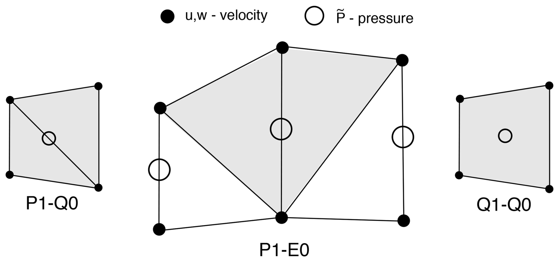
Figure A1 The P1–E0 element and two other secondary 2D elements that satisfy the solvability condition but possibly only in tests B and D^∗.

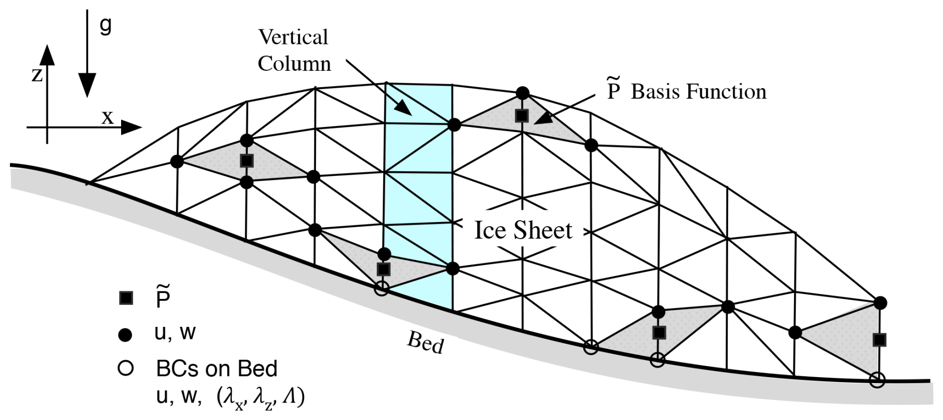
Figure A2 An illustration of a 2D edge-based P1–E0 mesh, composed of vertical columns randomly subdivided into triangles.

A2 Proving the solvability condition in P1–E0 element meshes

Consider a single vertical edge from top to bottom as in Fig. A2. Assuming m vertical edge segments, there will be m+1 discrete w variables and m discrete p variables since each p variable is located between a pair of w variables. However, since the w variable at the bottom is specified as a boundary condition, either as a no-slip condition or as a no-penetration condition, there will be only m unknown w variables. As a result, we have n_w=n_p along each vertical mesh edge and therefore over the entire mesh, thus satisfying the solvability condition. In case Lagrange multipliers are used, there will be m+1 unknown discrete w variables (since now the basal vertical velocity w is an unknown). However, this is matched by m unknown p variables, supplemented by one λ_z or one Λ unknown Lagrange multiplier variable, depending on the type of boundary condition. Thus, the number of unknown variables again equals the number of equations along every vertical edge, thereby satisfying the solvability condition. This means that the P1–E0 element can be used to satisfy the solvability condition irrespective of the boundary conditions on arbitrary meshes. These arguments will apply to other versions of the P1–E0 element as well, such as the second-order version of the P2–E1 element in Fig. 13a or the 3D version of the P1–E0 element in Fig. A3.

A3 Three-dimensional meshes based on the P1–E0 element

The two-dimensional P1–E0 element has a relatively simple three-dimensional counterpart, shown in Fig. A3. The mesh again consists of vertical columns, this time composed of hexahedra. Each hexahedron is subdivided into six tetrahedra such that each vertical edge is surrounded by as few as four to as many as eight tetrahedra. As in the 2D case, velocity components are collocated at vertices, yielding a piecewise linear velocity distribution in each tetrahedral element, and pressures are located in the middle of each vertical edge so that pressure is constant in the collection of tetrahedra that surround that edge. Lagrange multipliers, if used, are located at the vertices on the basal surface, yielding a piecewise linear distribution on the basal triangular facet. The solvability condition (58) is satisfied because the argument used in the 2D case applies here also since pressures and vertical velocities are again intermingled along a single line of vertical edges from top to bottom.

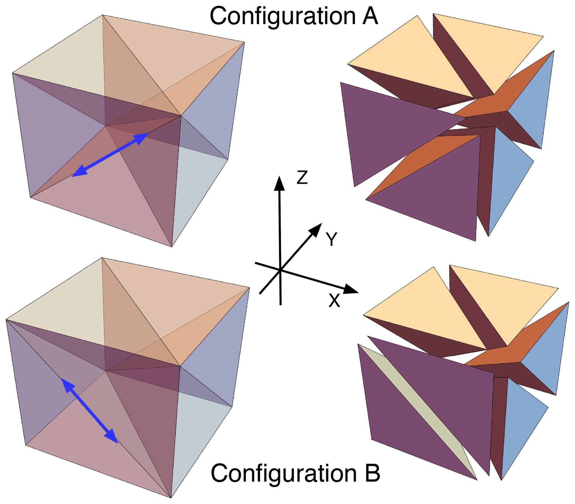
Figure A3 Three-dimensional P1–E0 tetrahedral elements that generalize the 2D P1–E0 element of Fig. A1. Configurations A and B differ by having an internal triangular face rotated, as indicated by the blue arrows. Both satisfy the solvability condition.

Figure A3 shows two of the several possible configurations of a typical hexahedron, including an exploded view of each configuration for clarity. The two configurations differ in having the internal face of the two forward-facing tetrahedra rotated, creating two different forward-facing tetrahedra. The remaining six tetrahedra are undisturbed. Since edges must align when hexahedra (or tetrahedra) are connected, this shows that the 3D mesh can be flexibly reconnected and rearranged, just as in the 2D case of Fig. A2.

A closely related and perhaps simpler three-dimensional P1–E0 element is based on a P2–P1 prismatic tetrahedral element discussed in Leng et al. (2012). A mesh of these elements is composed of vertical columns of prisms (with triangular faces at the top and bottom), each subdivided into three tetrahedra. Pressures are located on the vertical prism edges, as in Fig. A3, so this again satisfies the solvability condition.

Just as the 2D second-order P2–E1 element in Fig. 13a is a generalization of the P1–E0 element, a 3D second-order P2–E1 element may be constructed as a generalization of the P1–E0 element of Fig. A3. Velocities would be located at the vertices and at midpoints of the tetrahedral edges, and pressures would be located halfway between the velocities on vertical edges, including a set of imaginary vertical edges through the midpoints of the tetrahedral edges as in the 2D case in Fig. 13a. The P2–E1 element in both 2D and 3D will again satisfy the solvability condition since the arguments of Sect. B2 will also apply as pressures are located midway between vertical velocities along all vertical edges.

Appendix B: The inf-sup and solvability conditions

Recalling (47), the 2D Newton–Raphson iteration for saddle point problems is written as

$$\begin{array}{}\text{(B1)}& \begin{array}{rl}& \left[\begin{array}{lll}{\mathbf{M}}_{\mathrm{UU}}\left({\mathit{u}}^K,{\mathit{w}}^K\right)& {\mathbf{M}}_{\mathrm{UW}}\left({\mathit{u}}^K,{\mathit{w}}^K\right)& {\mathbf{M}}_{\mathrm{UP}}\\ {\mathbf{M}}_{\mathrm{UW}}^T\left({\mathit{u}}^K,{\mathit{w}}^K\right)& {\mathbf{M}}_{\mathrm{WW}}\left({\mathit{u}}^K,{\mathit{w}}^K\right)& {\mathbf{M}}_{\mathrm{WP}}\\ {\mathbf{M}}_{\mathrm{UP}}^T& {\mathbf{M}}_{\mathrm{WP}}^T& \mathrm{0}\end{array}\right]\left\{\begin{array}{l}\mathrm{\Delta }\mathit{u}\\ \mathrm{\Delta }\mathit{w}\\ \mathrm{\Delta }\mathit{p}\end{array}\right\}\\ & =\left\{\begin{array}{l}-R_U\left({\mathit{u}}^K,{\mathit{w}}^K,{\mathit{p}}^K\right)\\ -R_W\left({\mathit{u}}^K,{\mathit{w}}^K,{\mathit{p}}^K\right)\\ \mathrm{0}\end{array}\right\}.\end{array}\end{array}$$

In 3D the vector Δu will include the two horizontal increments, i.e., $\mathrm{\Delta }\mathit{u}\to {\left\{\mathrm{\Delta }\mathit{u},\mathrm{\Delta }\mathit{v}\right\}}^T$. For simplicity, if we rename quantities, (B1) may be put in the standard form (54) as follows:

$$\begin{array}{}\text{(B2)}& \left[\begin{array}{ll}\mathbf{A}& {\mathbf{B}}^T\\ \mathbf{B}& \mathrm{0}\end{array}\right]\left\{\begin{array}{l}\mathit{u}\\ \mathit{p}\end{array}\right\}=\left\{\begin{array}{l}\mathit{f}\\ \mathit{g}\end{array}\right\},\end{array}$$

where

$$\begin{array}{rl}\stackrel{\mathrm{̃}}{\mathit{u}}& ={\left\{\mathrm{\Delta }\mathit{u},\mathrm{\Delta }\mathit{w}\right\}}^T,\mathbf{A}=\left[\begin{array}{l}{\mathbf{M}}_{\mathrm{UU}}\left({\mathit{u}}^K,{\mathit{w}}^K\right){\mathbf{M}}_{\mathrm{UW}}\left({\mathit{u}}^K,{\mathit{w}}^K\right)\\ {\mathbf{M}}_{\mathrm{UW}}^T\left({\mathit{u}}^K,{\mathit{w}}^K\right){\mathbf{M}}_{\mathrm{WW}}\left({\mathit{u}}^K,{\mathit{w}}^K\right)\end{array}\right],\\ \mathbf{B}& =\left[{\mathbf{M}}_{\mathrm{UP}}^T{\mathbf{M}}_{\mathrm{WP}}^T\right],\end{array}$$

and similarly for other variables.

As noted earlier, matrix A is invertible. Solving for and eliminating u in (B2), one obtains an equation for the pressure,

$$\begin{array}{}\text{(B3)}& \left({\mathbf{BA}}^{-\mathrm{1}}{\mathbf{B}}^T\right)\mathit{p}=\left({\mathbf{BA}}^{-\mathrm{1}}\right)\mathit{f},\end{array}$$

where $\mathit{S}=\left({\mathbf{BA}}^{-\mathrm{1}}{\mathbf{B}}^T\right)$ is the Schur complement with respect to p. This equation may be solved for p provided an inf-sup condition on matrix B^T is satisfied (Benzi et al., 2005; and more specifically see the lecture notes by Jean-Frédéric Gerbeau for course CME358, Stanford University, Chap. 3 (in particular Remarks 3.2 and 3.3), available at https://web.stanford.edu/class/cme358/notes/cme358_lecture_notes_3.pdf, last access: 4 September 2025). Having solved for p, the velocity u is obtained as follows:

$$\begin{array}{}\text{(B4)}& \mathit{u}={\mathbf{A}}^{-\mathrm{1}}\left(\mathit{f}-{\mathbf{B}}^T\mathit{p}\right).\end{array}$$

This is generally not a practical solution method since the Schur complement matrix S is dense, and therefore it is too expensive to solve. In particular, Gerbeau shows that the standard inf-sup condition for B^T is equivalent to the much simpler condition,

$$\begin{array}{}\text{(B5)}& \mathrm{Ker}{\mathbf{B}}^T=\left\{\mathrm{0}\right\},\end{array}$$

which is called the “algebraic inf-sup condition”. In other words, the inf-sup condition is equivalent to requiring the null space of B^T to be the zero vector, which means that the solution for pressure must not contain spurious modes. This suggests that the existence of a pressure null space is the culprit in the need to satisfy the inf-sup condition.

Now consider the situation when the Newton–Raphson system (B1) is solved with a mesh satisfying the solvability condition. Simplifying notation as before, the linear system (B1) may be written as follows:

$$\begin{array}{}\text{(B6)}& \left[\begin{array}{lll}{\mathbf{M}}_{\mathrm{UU}}& {\mathbf{M}}_{\mathrm{UW}}& {\mathbf{M}}_{\mathrm{UP}}\\ {\mathbf{M}}_{\mathrm{UW}}^T& {\mathbf{M}}_{\mathrm{WW}}& {\mathbf{M}}_{\mathrm{WP}}\\ {\mathbf{M}}_{\mathrm{UP}}^T& {\mathbf{M}}_{\mathrm{WP}}^T& \mathrm{0}\end{array}\right]\left\{\begin{array}{l}\mathit{u}\\ \mathit{w}\\ \mathit{p}\end{array}\right\}=\left\{\begin{array}{l}{\mathit{f}}_U\\ {\mathit{f}}_W\\ \mathrm{0}\end{array}\right\}.\end{array}$$

As shown in Sect. 4.3.2, if the solvability condition applies, then matrices ${\mathbf{M}}_{\mathrm{WP}},{\mathbf{M}}_{\mathrm{WP}}^T$ are invertible, and the continuity equation, the third equation in (B6), may be solved for the vertical velocity w, as in (56). Using (56) in the functional (59) one obtains (60), an equation for u only. With a bit of algebra, and using (56) in (B6), the corresponding linear equation for u is given by

$$\begin{array}{}\text{(B7)}& \begin{array}{rl}& \left({\mathbf{M}}_{\mathrm{UU}}-\left({\mathbf{M}}_{\mathrm{UW}}-{\mathbf{M}}_{\mathrm{UP}}{\mathbf{M}}_{\mathrm{WP}}^{-\mathrm{1}}{\mathbf{M}}_{\mathrm{WW}}\right){\mathbf{M}}_{\mathrm{WP}}^{-T}{\mathbf{M}}_{\mathrm{UP}}^T\right.\\ & \left.-{\mathbf{M}}_{\mathrm{UP}}{\mathbf{M}}_{\mathrm{WP}}^{-\mathrm{1}}{\mathbf{M}}_{\mathrm{UW}}^T\right)\mathit{u}=\left({\mathit{f}}_U-{\mathbf{M}}_{\mathrm{UP}}{\mathbf{M}}_{\mathrm{WP}}^{-\mathrm{1}}{\mathit{f}}_W\right).\end{array}\end{array}$$

As pointed out in Sect. 4.3.2, this is a well-behaved and stable equation for u. However, just as was the case with (B3), the associated matrix is dense and too expensive to solve in practice. Nevertheless, with u obtained from solving (B7), the second equation of (B6) yields the following matrix equation to be solved for the pressure p,

$$\begin{array}{}\text{(B8)}& {\mathbf{M}}_{\mathrm{WP}}\mathit{p}=\left({\mathbf{M}}_{\mathrm{WW}}{\mathbf{M}}_{\mathrm{WP}}^{-T}{\mathbf{M}}_{\mathrm{UP}}^T-{\mathbf{M}}_{\mathrm{UW}}^T\right)\mathit{u}+{\mathit{f}}_W.\end{array}$$

Thus, corresponding to equations (B4) and (B3), one obtains equations (B7) and (B8), but this time to be solved in reverse order, first for velocity u and then for the pressure p. The essential difference between the equations for pressure, (B3) and (B8), is that in (B3) the Schur complement matrix S requires the inf-sup condition to be satisfied, while in (B8) there is no such requirement for matrix M_WP. Thus, pressure solutions will be well behaved with no spurious pressure modes, although there is no guarantee or expectation of smoothness. This implies that the solvability condition (58), and more importantly the invertibility of matrix ${\mathbf{M}}_{\mathrm{WP}}^T$, is sufficient for the well posedness of the Stokes saddle point problem.

Appendix C: Test problems

We shall use three 2D test problems to demonstrate the new methods. The geometrical configuration of the three problem meshes is illustrated in Fig. C1. The first problem, named Test B, is actually Exp. B from the ISMIP-HOM benchmark suite (Pattyn et al., 2008); it features a no-slip condition on a sinusoidal basal surface. The second problem, Test D^∗, incorporates sinusoidal friction along a uniformly sloped plane basal surface. This is a modification of Exp. D from the benchmark suite but with increased friction since ice flow in Exp. D is very nearly vertically constant (see Fig. 4) and is characteristic of the shallow-shelf regime, which is not of present interest.

A third problem, Test O (for “obstacle”) is introduced to illustrate the adaptive switching discussed in Sect. 6.1. As illustrated in Fig. C1, Test O has a unique feature, a thin no-slip obstacle, located at x=4 km and extending vertically 200 m from the bed (20 % of the ice sheet thickness), which forces ice flow near the obstacle to adjust abruptly. However, there is a problem if a triangulation like the one in tests B or D^∗ were to be used. This is because the no-slip boundary conditions in the triangular element in the lee of the obstacle, with one vertical edge and one edge along the bed, would result in all vertex velocities being zero. This would imply zero stress and therefore a singularity in ice viscosity. To avoid this, elements at the back of the obstacle are “reversed” compared to the ones at the front of the obstacle, as shown in Fig. C1.

Figure C1 Test problem meshes. For clarity, a coarse 5×5 configuration is shown.

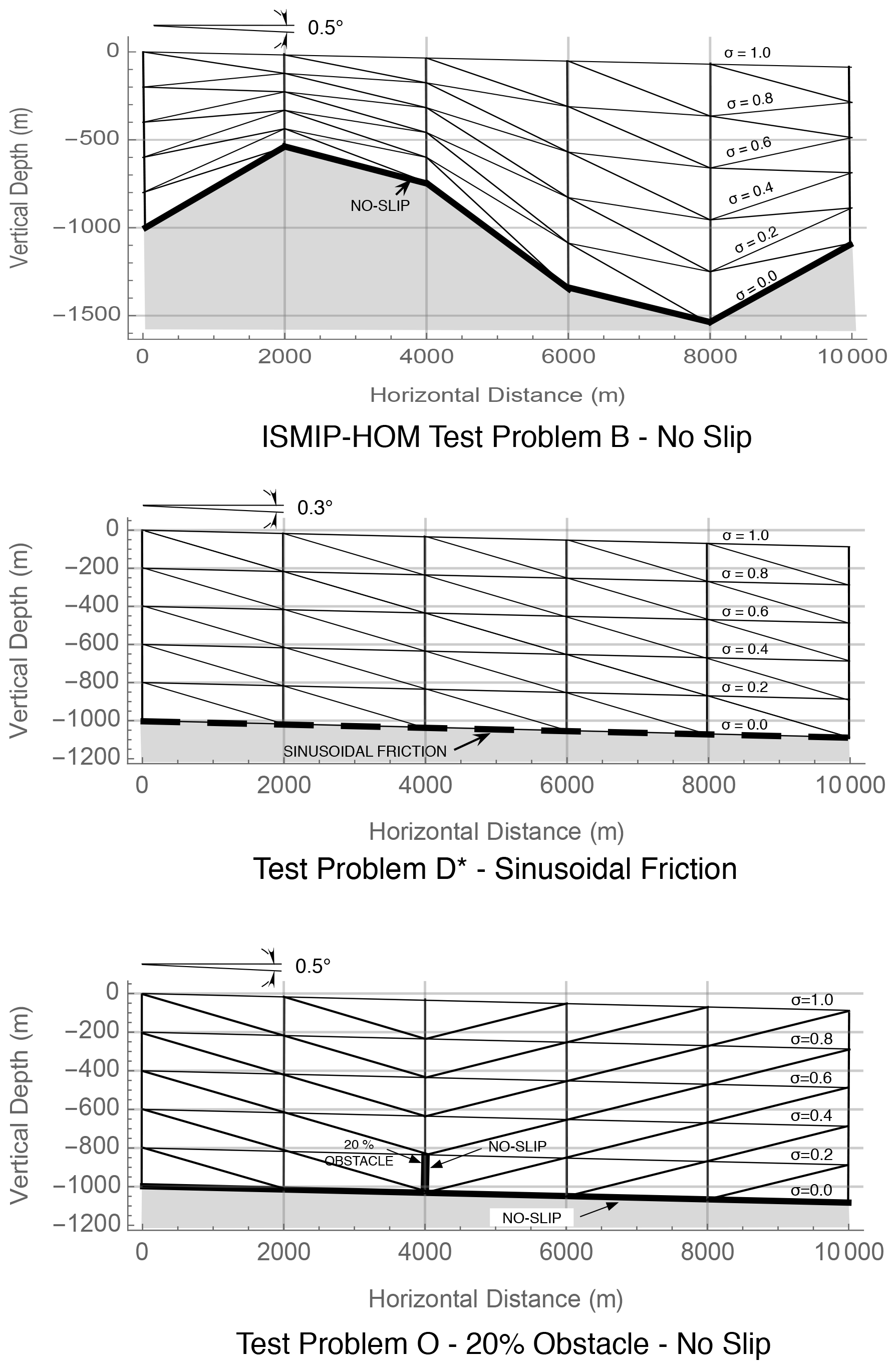
All tests feature a sloping flat upper surface, given by $z_s\left(x\right)=-\mathrm{xTan}\left(\mathit{\theta }\right)$, where θ=0.5^° for tests B and O and θ=0.3^° for Test D^∗ (this is different from the 0.1^° slope in Test D), with stress-free boundary conditions. The bottom surface elevation in Test B is given by $z_b\left(x\right)=z_s\left(x\right)-H_{\mathrm{0}}+H_{\mathrm{1}}\mathrm{Sin}\left(\mathit{\omega }x\right)$, where H₀=1000 m, H₁=500 m, $\mathit{\omega }=\mathrm{2}\mathit{\pi }/L$, and L is the perturbation wavelength or the domain length. The length L in the ISMIP-HOM suite ranges from 5 to 160 km, but here we consider only three cases at the high end of the aspect ratio ($H_{\mathrm{0}}/L)$ range, namely $L=\mathrm{2},\mathrm{5},\mathrm{10}$ km, where the inaccuracy of the Blatter–Pattyn approximation becomes noticeable. The bottom surface elevation in tests D^∗ and O is $z_b\left(x\right)=z_s\left(x\right)-H_{\mathrm{0}}$, parallel to the upper surface. The spatially varying friction coefficient for Test D^∗ is $\mathit{\beta }\left(x\right)={\mathit{\beta }}_{\mathrm{0}}+{\mathit{\beta }}_{\mathrm{1}}\mathrm{Sin}\left(\mathit{\omega }x\right)$, where ${\mathit{\beta }}_{\mathrm{0}}={\mathit{\beta }}_{\mathrm{1}}={\mathrm{10}}^{\mathrm{4}}$ Pa a m⁻¹ (this is an order of magnitude larger than in Test D). Lateral boundary conditions are periodic. Physical parameters are the same as in ISMIP-HOM, i.e., ice flow parameter $A={\mathrm{10}}^{-\mathrm{16}}$ Pa⁻³ a⁻¹, ice density ρ=910 kg m⁻³, and gravitational constant g=9.81 m s⁻². In general, units are MKS, except time is usually per annum, convertible to per second by the factor 3.1557×10⁷ s a⁻¹.