SPASS – new gridded climatological snow datasets for Switzerland: potential and limitations

Gridded information on the past, present, and future state of the surface snow cover is an indispensable climate service for any snow-dominated region like the Alps. Here, we present and evaluate the first long-term gridded datasets of daily modeled snow water equivalent and snow depth over Switzerland, available at 1 km spatial resolution since 1962 (spanning 60+ years). These climate-oriented datasets are derived from a quantile-mapped temperature index model (OSHD-CLQM). The validation against a higher-quality but shorter-duration dataset – derived from the same model but enhanced with data assimilation via an ensemble Kalman filter (OSHD-EKF) – shows, on the one hand, good results regarding bias and correlation and, on the other hand, acceptable absolute and relative errors except for ephemeral snow and for shorter time aggregations like weeks. An evaluation using in situ station data for yearly, monthly, and weekly aggregations at different elevation bands shows only slightly better performance scores for OSHD-EKF, highlighting the effectiveness of the quantile-mapping method used to produce the long-term climatological OSHD-CLQM dataset. For example, yearly maps of gridded snow depth compared to in situ data demonstrate an RMSE of 25 cm (20 %) at 2500 m and of 1.5 cm (80 %) at 500 m. For monthly averages, these numbers increase to 30 cm (25 %) and 3 cm (100 %), respectively. A trend analysis of yearly mean snow depth from these gridded climatological- and station-based data revealed very good agreement on direction and significance at all elevations. However, at the lowest elevations the strength of the decreasing trend in snow depth is clearly overestimated by the gridded datasets. Moreover, a comparison of the trends between individual stations and the corresponding grid points revealed a few cases of larger disagreements in the direction and strength of the trend. Together these results imply that the performance of the new snow datasets is generally encouraging but can vary at low elevations, at single grid points, or for short time windows. Therefore, despite some limitations, the new 60+-year-long OSHD-CLQM gridded snow products show promise as they provide high-quality and spatially high-resolution information on snow water equivalent and snow depth, which is of great value for typical climatological products like anomaly maps or elevation-dependent long-term trend analysis.

1 Introduction

Snow cover is an integral and crucial component of the Earth's energy and water balance. It reacts sensitively to climate change due to its dependence on precipitation and temperatures below freezing. Climate changes lead to changes in the extent, thickness, density, optical, and thermal properties of the snow cover and thus of the Earth's surface and the boundary layer between the Earth and the atmosphere (Abe, 2022). These changes have far-reaching consequences for glaciers, extreme events, natural hazards, ecosystems, biodiversity, forests, and landscapes, as well as for winter sports and the tourism industry, both globally and regionally (Mote et al., 2018; López-Moreno et al., 2020; Bozzoli et al., 2024). This also includes the impact on water resources for irrigation, drinking water, and hydropower (IPCC, 2019). Snow as frozen precipitation is of increasing importance globally in a world facing more frequent droughts on the one hand and more extreme precipitation events on the other, where snow can dampen immediate runoff but can also cause avalanches or flooding (Barnett et al., 2005). Accurate information about the past and current evolution of the snow cover is therefore of high importance (van Ginkel et al., 2020).

In contrast to the hemispheric level (Mortimer et al., 2020) or other countries (Olefs et al., 2020), Switzerland so far has provided long-term snow cover information based on in situ data for daily snow depth (Marty and Blanchet, 2012; Scherrer et al., 2013; Schmucki et al., 2017) and biweekly water equivalent of the snow cover (SWE) from national monitoring networks (Marty et al., 2023), which are only available at about 10 % of the snow depth measuring stations. Both types of data, snow depth (HS) and SWE, are regularly published in the annual winter reports (Pielmeier et al., 2024) and in online repositories (Marty, 2020). Such point-based time series are very valuable because of their lengths and documented measurement history (Buchmann et al., 2022). However, even though Switzerland has a high density of snow measurement stations, their asymmetric distribution (especially in terms of altitude) and irregular temporal availability (some had to be abandoned, others recently started from scratch due to automation) limit their usefulness for climatological applications beyond station-based analyses, i.e., the provision of altitude-dependent region- or country-wide snow information.

Ideally, snow data would be available on a daily scale in a gridded format for many decades. Using interpolated station data for this purpose (Luomaranta et al., 2019) has several disadvantages because of the abovementioned asymmetric distribution and irregular temporal availability of station series. Using remote sensing data (Poussin et al., 2025) is another option but is hampered by irregular temporal availability (among others due to cloud coverage) and possible inhomogeneities (due to different satellite generations) and limits the start of the time period to the beginning of the 1980s. A third and often used option is the use of model or reanalysis data, which are often only available at relatively coarse spatial resolution. In a recent study, Scherrer et al. (2024) evaluated the usefulness of existing long-term and spatially gridded SWE datasets for Switzerland. Among others, the authors state that most datasets, including the high-resolution ones, have problems correctly representing small SWE values at low elevations, and they conclude that a kilometer-scale model with assimilated snow measurement data is highly preferable. The only model in this investigation which fulfilled these requirements was the temperature index model OSHD-EKF, which is also used in this study as a benchmark dataset for the evaluation.

This model is operated by the Operational Snow Hydrological Service (OSHD) at the WSL Institute for Snow and Avalanche Research (SLF), hereafter referred to as OSHD-EKF, and provides daily 1 km gridded information on SWE between 1999 and today (for details see Mott et al., 2023). The length of this dataset is limited back to 1999 because there are not enough high-elevation snow stations available for assimilation before that time. To overcome this limitation and make use of the full period of available gridded datasets (1962 to today), we developed within the project SPAtial Snow climatology for Switzerland (SPASS) the quantile-mapping procedure SnowQM, which was presented in Michel et al. (2024). This method allows correcting the non-data-assimilated full climatological SWE time series starting in the hydrological year 1962 (OSHD-CL) into a better-quality dataset (OSHD-CLQM), which mimics the higher-quality shorter-duration OSHD-EKF model. For the development of OSHD-CLQM, the quantile-mapping method SnowQM was calibrated and validated with SWE simulations between 1999 and 2021 using the OSHD-EKF dataset as a target and was then applied to the OSHD-CL dataset over the period from the hydrological year 1962 to today (Fig. 1).

Michel et al. (2024) concluded that the developed quantile-based correction can efficiently reduce the pronounced SWE bias at high elevations and that the average bias is always close to zero. Moreover, they stated that the mean absolute error can remain large even after correction and that SnowQM is not expected to do more than a climatological bias correction, meaning that biases at short timescales, like a single day or month, are not necessarily corrected. Additionally, they mentioned that such biases can also concern entire winters in low-elevation regions. However, quantitative information on elevation-dependent uncertainties is not provided but is important in mountain regions (Switanek et al., 2024). Moreover, the abovementioned OSHD datasets only contain SWE as a snow variable. However, SWE is an unusual and elusive variable for the non-scientific public (e.g., tourism, media), and many applications explicitly need snow depth (HS).

The novelty of our study is therefore, first, the creation of the corresponding gridded datasets for snow depth by applying the SWE2HS algorithm developed by Aschauer et al. (2023). Second, we compared the OSHD-CLQM datasets to the higher-quality OSHD-EKF and station-based datasets to investigate potential time-aggregation- and elevation-dependent biases. Third, we also analyzed differences in long-term trends to get a clearer picture of the potential and limitations of the datasets. These three aspects combined allow us to provide an unprecedented long-term gridded snow depth dataset and assess its utility across a range of potential use cases. In Sect. 2, we first present the gridded and station data used, as well as the evaluation methods applied. In Sect. 3, we explain and discuss the results before summarizing our findings in Sect. 4.

2 Data and methods

2.1 Spatial SWE and HS datasets

As illustrated in Fig. 1, the base dataset is OSHD-CL, which provides SWE and is based on a temperature index model forced by gridded temperature (TabsD: MeteoSwiss, 2021a) and precipitation (RhiresD: MeteoSwiss, 2021b) input fields at 1 km spatial resolution as well as an algorithm for the fraction of snow-covered area (Magnusson et al., 2014). As a target for the quantile mapping, we use the higher-quality but shorter (1999–2023) OSHD-EKF dataset as a benchmark. This dataset was created using the same model and data but also assimilating snow data from a time-invariant set of 350 in situ snow stations using an ensemble Kalman filter (Magnusson et al., 2014). In a next step, the data were corrected by the SnowQM algorithm so that OSHD-CLQM data finally consist of 1 km daily gridded quantile-mapped SWE data over the domain of Switzerland between 1962 and 2023 (Michel et al., 2024). The analyses are performed for hydrological years, lasting from September of the previous year to August of the year of investigation. The hydrological year 2023, for instance, consists of the period 1 September 2022 to 31 August 2023. This definition is consistent with the settings of the OSHD models, which sets SWE to zero on 1 September of each year to only represent seasonal snow, thus operating on an annual cycle starting in September. The corresponding spatial snow depth datasets were derived by applying the SWE2HS algorithm (Aschauer et al., 2023) to the SWE data from both models (OSHD-CLQM and OSHD-EKF). This algorithm contains a multilayer snow density model which uses daily SWE as the sole input.

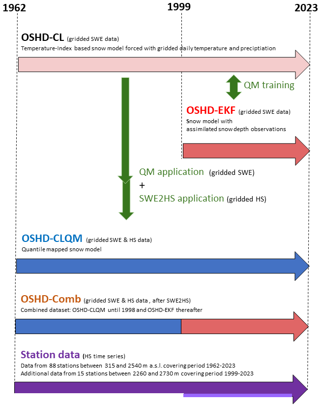
Figure 1 Conceptual view of the workflow of the different model and station datasets used as well as for which periods they are available.

2.2 Reference datasets

To evaluate the performance of the long-term OSHD-CLQM dataset, we use as two references: (1) the higher-quality OSHD-EKF dataset, which limits the comparison to the 1999–2023 period, and (2) daily in situ station data, which limit the comparison to snow depth.

It is important to mention that OSHD-CLQM is not independent of the first reference as OSHD-EKF was used in the above-described quantile-mapping step to produce OSHD-CLQM (Sect. 2.1). Additionally, some uncertainty is expected when comparing HS data, as this variable is only available for both datasets through the conversion of SWE using the SWE2HS algorithm (Aschauer et al., 2023), which may introduce additional errors, particularly in challenging conditions such as rain-on-snow events.

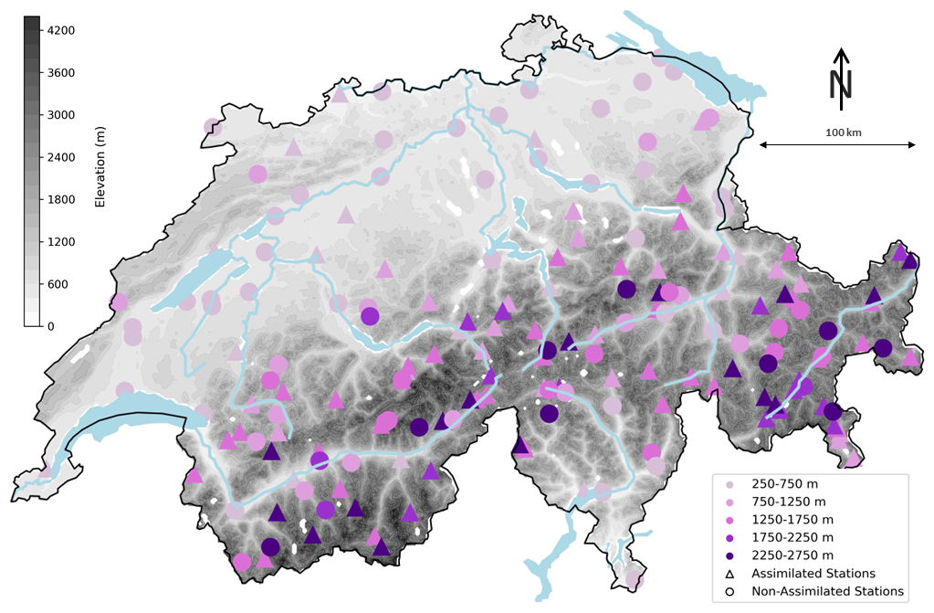
Figure 2 Map of Switzerland with the elevation of the individual grid points and the distribution of stations used to validate the gridded datasets. Stations are colored by elevation band; assimilated stations (OSHD-EKF) are shown as triangles and non-assimilated stations as circles.

When comparing to in situ data we have to take into account the common grid-to-point mismatch problem. In this regard, it is important to know that both datasets (CLQM and EKF) are based on the OSHD temperature index model (OSHD-CL), which was run in its default mode, where the SWE values represent the spatial mean of the respective 1 km grid cells, considering its predominant land cover types and terrain characteristics. This is in line with the OSHD's objective of conducting a comprehensive assessment of snow and water resources in Switzerland, but it entails issues when comparing to in situ data, which represent snow conditions at flat, non-forested, sheltered field sites according to international measurement standards (WMO, 2024a). Indeed, the monitoring sites have been reported to often systematically overrepresent snow depth (Grünewald and Lehning, 2015), and hence negative biases of OSHD-EKF relative to station data are expected, which must be kept in mind when interpreting respective results. Moreover, elevations above 3000 m are not analyzed as grid points above this elevation are sometimes affected by too much snow accumulation in the model due to the lack of high-elevation station data for assimilation into the model (Michel et al., 2024).

As daily in situ snow depth time series, we use, on the one hand, data from 103 stations (Table S1 in the Supplement), which have already been used in the assimilation procedure of OSHD-EKF (Fig. 1) and are therefore complete between 1999 and 2023. On the other hand, for an independent analysis (Fig. 6), we use data from 79 independent stations, which have not been used in the data assimilation step because they cover only part of the time between 1999–2023. All stations are located between 200 and 2800 m a.s.l. (Fig. 2); stations below 2000 m consist of manual measurements only and stations above 2000 m mostly consist of automatic measurements. The data from these stations have been carefully quality-controlled (physical threshold checks, as well as temporal and spatial consistency checks) and gap-filled (Aschauer and Marty, 2021). Each station is compared with its most representative grid point, which was determined based on the selection of the grid cell that contains the station of interest as well as the eight surrounding grid cells. The grid cell with the smallest elevation difference from the station was chosen for the comparison as snow depth is generally strongly dependent on elevation (Marty and Blanchet, 2012). The median elevation difference between the station and the selected grid cell over all stations is 10 m with a standard deviation of 23 m; the largest elevation difference is 105 m. The digital elevation model to determine the grid point elevation was provided by swisstopo (2017).

2.3 Spatial and temporal aggregations

Michel et al. (2024) demonstrated that the SWE bias of OSHD-CLQM is not remarkably different between north and south of the Alps, which are the two main climatic regions in Switzerland. We focus here on elevation-dependent biases, as the existence of snow in the Alps strongly depends on the elevation above sea level (Schöner et al., 2019; Switanek et al., 2024). For this purpose, we use elevation bands with a width of ±250 m, which are centered at 500, 1000, 1500, 2000, and 2500 m. Therefore, we also pool the abovementioned station data into these elevations bands with the goal of comparing all corresponding grid points in an elevation band to all stations in this elevation band (Tables S1 and S2).

These elevation bands imply that grid points below 250 m and above 2750 m were not evaluated when comparing with station data because there are hardly any stations for assimilation or validation available below and above these thresholds. Additionally, there are hardly any grid points below 250 m in the domain of Switzerland (see Table S2).

To assess time-aggregation-dependent biases, we use aggregations of the daily data to weekly, monthly, and yearly mean values. The motivation behind the temporal units used was given by the following: climatological analyses are often provided by yearly or monthly reports and we wanted to assess the uncertainty of the new snow products with the goal of including them in future reports. Moreover, knowing about the need for timely public information on possible current extraordinary snow conditions, we also assessed the weekly aggregation level. Daily aggregations were by purpose not assessed as the quantile-mapping method at this scale can be associated with substantial uncertainties and an interpretation of the results at this high temporal resolution is not recommended (Michel et al., 2024). Yearly mean values are based on the 6-month period between November and April, which we will refer to as “yearly” from now on because it is the period where snow cover is predominant in most of the regions in the country and because it is the period where manual snow depth measurements are available completely. To compute yearly, monthly, or weekly mean values, we always first averaged each grid point over time for each elevation band. This means that box plots show the variability across space in each elevation band for each temporal aggregation. In the case of model-to-station intercomparison (Figs. 5, S3), the box plots were created based on the number of stations per elevation band (as listed in Table S2).

Moreover, we evaluate time-aggregation- and elevation-dependent biases of commonly used climatological anomalies. For this purpose, the 30-year average between 1991 and 2020 (standard 30-year reference period) is calculated for every grid point and the ratio between the weekly, monthly, or yearly mean values and its reference period is determined. When investigating performance differences between OSHD-CLQM and OSHD-EKF the evaluation is necessarily based on the period 1999–2023, which also has the advantage of having more in situ data (Table S2) available in the different elevation bands (mean per elevation band is 20 stations, minimum 14 stations, maximum 34 stations).

2.3.1 Merging gridded datasets for trend analysis

It is not surprising and there are clear indications that the climatologies of OSHD-CLQM and OSHD-EKF are not that different (Fig. S1 in the Supplement). Hence, we also constructed a new “combined” time series, OSHD-Comb (Fig. 1), by concatenating the first part of OSHD-CLQM (1962–1998) with OSHD-EKF (1999 and 2023). This approach allows investigating the impact on trends when merging the best available datasets for each period.

Long-term trends of all the abovementioned time series are evaluated based on yearly values with the Theil–Sen slope (Theil, 1950; Sen, 1968) and the Mann–Kendall (MK) trend test (Mann, 1945). A positive standardized MK value indicates an increasing trend, while a negative value demonstrates a decreasing one. Confidence levels of 95 % are used as a threshold to classify a significant trend (p<0.05). The Theil–Sen slope estimator provides a measure of the strength of a trend based on a robust simple nonparametric linear regression. Absolute trends were always calculated as change per decade and relative trends were calculated for the entire 62-year period as percentage changes between 1962 and 2023 based on the Theil–Sen slope. Please keep in mind that a direct comparison of percentage changes is only meaningful between indicators of the same unit and similar absolute values. The thus calculated trends of the model datasets are also compared to the trends from in situ station data. The stations available for this comparison cover all elevation levels quite well (Table S2). The same stations are available for each elevation band as for the 1999–2023 comparison, except for the highest elevation band (2250–2750 m a.s.l.), where only one station covers the required full period between 1962 and 2023.

2.4 Evaluation metrics

The analyses are mainly based on the two variables describing the mass and depth of snow cover: SWE in millimeters and HS in centimeters. Moreover, we also analyze the number of snow days. We define three different classes of snow days: days with snow cover of at least 5, 30, or 50 cm of snow depth.

We use four statistical evaluation scores to compare the various datasets to evaluate the gridded snow products: root mean squared error (RMSE), mean bias (BIAS), correlation coefficient (R), and mean arctangent absolute percentage error (MAAPE).

MAAPE (Kim and Kim, 2016) is an adaptation of the mean absolute percentage error (MAPE) to mitigate large percentage errors occurring only due to small reference values. To get MAAPE, first, like in the case of MAPE, the absolute relative difference between the target value ($\widehat{y}$) and the reference value (y_i) is calculated.

$$\begin{array}{}\text{(1)}& \mathrm{MAAPE}={\displaystyle \frac{\mathrm{1}}{n}}\sum _{i=\mathrm{1}}^n\arctan \left(\left|{\displaystyle \frac{y_i-{\widehat{y}}_i}{y_i}}\right|\right)\end{array}$$

But then the arctan of this relative difference is taken, which maps large values to [$\mathrm{0};\mathit{\pi }/\mathrm{2}$] and hence limits the maximum relative error to 157 %. When we write about relative errors in the “Results and discussion” section, we always refer to MAAPE values for better readability. The scores provide the basis for box plots of RMSE, bias, R, and MAAPE in each elevation band (500, 1000, 1500, 2000, 2500 m) for each temporal aggregation (see also Sect. 2.3).

3 Results and discussion

3.1 Analysis of performance scores based on gridded reference dataset

In order to quantify time- and elevation-dependent uncertainties arising from the quantile mapping, we first evaluated the OSHD-CLQM model simulation against the OSHD-EKF model simulations used as the target dataset (Fig. 3). As expected from the quantile-mapping procedure (Cannon et al., 2015), bias for SWE is close to zero for all temporal aggregations and all elevation bands. HS, however, reveals a slightly negative bias (ca. −2 cm) for the highest elevation band because HS has been derived from SWE by conversion using SWE2HS and therefore has not been directly mapped to match the quantile distributions of the observed snow depth measurements. For both variables SWE and HS, RMSE and MAAPE demonstrate a moderate worsening of the score performance for all elevations with temporal aggregation over smaller periods, illustrated, e.g., by RMSE values at 1500 m increasing from 21 to 31 mm SWE or 7 to 11 cm HS going from yearly to weekly aggregation. Regarding elevation dependence, RMSE increases up to 2000 m, but MAAPE and R reveal a clear improvement in score performance when going from low to high elevations. Indeed, MAAPE scores demonstrate for SWE and HS at 500 m values of about 37 % for yearly resolution. At the same time, at 2500 m MAAPE is about 8 % at yearly resolution. The same general performance increase in MAAPE with elevation is also true for monthly and weekly aggregations, which are about 58 % and 65 % at 500 m and decrease to 11 % and 13 % at 2500 m. All these comparisons demonstrate that the performance generally increases with elevation in all evaluation metrics, except bias, which is close to zero anyway. The main reason for this better performance with increasing elevation is the fact that the error indices in this analysis reflect the performance of the quantile-mapping step, which is not really suitable for time series with many zero values, i.e., for regions where the snow cover only survives for a few days at a time (Michel et al., 2024). Moreover, the signal-to-noise ratio of the quantile mapping increases with elevation due to the larger absolute amount of snow.

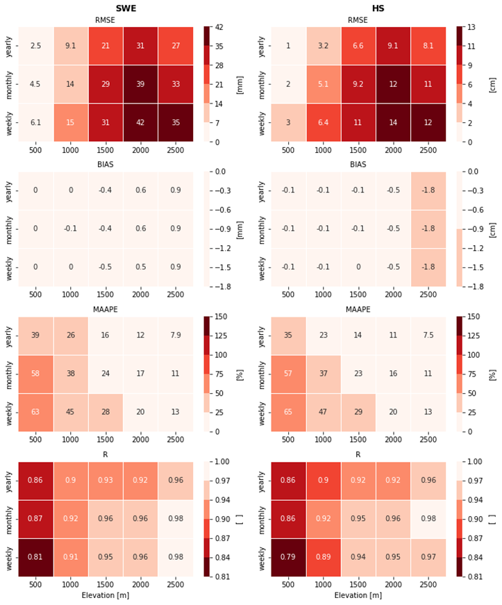
Figure 3 Heatmap of mean SWE (left) and HS (right) evaluation scores for the gridded OSHD-CLQM dataset in the period 1999–2023 using the OSHD-EKF dataset as a reference. Darker shades of red indicate worse scores.

In a second step, we investigated the distribution of the performance scores with the help of box plots for the same temporal aggregations and elevation bands. Figure 4 shows the corresponding box plots for both snow variables. While mean values of bias are close to zero for all elevations bands, whiskers and outliers demonstrate a clear increase in variability of the yearly values with increasing elevation. Larger bias can occur above 2750 m (not shown), where no in situ data for assimilation are available but where such differences are still small in relative terms. This can also be seen by the low MAAPE values in the highest elevation band. In contrast, at 500 m MAAPE values demonstrate that the relative error is on average about 40 % but can be as high as 70 % in rare cases. Similarly, R values show a clear increase in the spread with decreasing elevation.

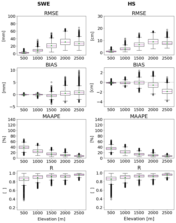
Figure 4 Score comparison between models OSHD-CLQM and OSHD-EKF (“reference”) at a yearly resolution at respective elevation bands (m) for SWE (left) and HS (right). Box plots were generated from these performance scores to illustrate the distribution, outliers, mean (green triangle), and median (purple line). The box reflects the 50 % of data between the lower quartile and upper quartile. The whiskers extend from the boxes' edges and correspond to 1.5 IQR. Outliers are represented as individual dots.

The same analysis as in Fig. 4 has been undertaken for monthly and weekly performance scores (Fig. S2). Monthly scores reveal the highest RMSE values at 2000 m of about 10 to 70 mm SWE (based on whiskers) or 5 to 20 cm HS, which according to MAAPE corresponds to a relative error range of 5 to 25 % for HS and SWE. However, in extremes cases (outliers) this error can be as high as 40 %. At 500 m the MAAPE whisker range goes from 40 % to 80 % for both snow variables but can go up to about 90 % in extreme cases for both variables. This low performance in these extreme cases in this elevation band is also illustrated by accordingly low R scores of about 0.4 for both variables. Weekly scores demonstrate a similar pattern but slightly lower performance for RMSE and MAAPE for both variables SWE and HS. The highest relative errors scores (but with small absolute errors) can again be seen in the lowest elevation band with a MAAPE whisker range demonstrating values between 50 % and 80 %. A clearly lower performance for weekly scores can also be seen for R, where in extreme cases values of only 0.2 are found. These lowest R scores usually originate from the few lowest grid points in this elevation band. These lowest grid points are located in separate regions north and south of the main Alpine ridge, which are often characterized by opposing snow conditions (Scherrer and Appenzeller, 2006); i.e., one region has snow and the other not. This possible divergence is smaller for yearly values as there is a higher chance for compensation than for monthly or weekly values.

3.2 Analysis of performance scores based on in situ station data as a reference

After investigating differences between the OSHD-CLQM and OSHD-EKF models, we now compare HS simulations of the two gridded models with HS observations at the stations. Note that point observations do not necessarily represent spatial means over large grid cells, particularly in complex and steep terrain, and a comparison to results from a model that represents the existing sub-grid variability is hence confounded.

Figure 5 illustrates that the yearly scores between the stations and the respective model grid points of OSHD-CLQM and OSHD-EKF show remarkable similarity overall. However, R values of OSHD-EKF stand out as being more consistent and are found to be higher in all elevation bands, especially at lower elevations. As expected for a model that assimilates snow observations, OSHD-EKF demonstrates slightly better comparison statistics, but the differences are minor, which attests to the good performance of the quantile-mapping procedure. Both models show larger bias values at higher elevations, peaking in the highest elevation band with median values of about −20 cm, which indicates that, as expected, the two models feature less snow at the highest elevations compared to the station values. There are several reasons for these bias values. First, data from flat field observations at high elevation often show larger values than the surrounding area (Grünewald and Lehning, 2015). Second, the SWE2HS algorithm sometimes tends to underestimate HS at these elevations (Aschauer et al., 2023). And third, there is a lack of stations for assimilation at high elevation (Mott et al., 2023). In relative terms, this bias, which is reflected in the MAAPE score, reveals errors between 20 % and 25 % at the elevation band 1500 m and above. This is in strong contrast to the values of about 80 % at the 500 m elevation band owing to the very low mean snow depths at these elevations.

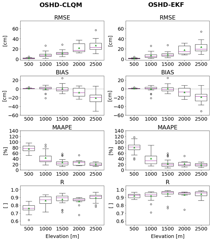
Figure 5 Score comparison between station data and OSHD-CLQM (left) as well as OSHD-EKF (right) in the respective elevation bands for yearly snow depth values. The median value is illustrated as a purple line and the mean value as a green triangle.

The same analysis has been undertaken for monthly and weekly performance scores (Fig. S3) and generally reveals the same pattern (lower performance for smaller time aggregations) as found when intercomparing the two models, with the difference that the performance decrease going from yearly to monthly or weekly time windows is now much weaker. OSHD-EKF stands out again with higher R values, especially at lower elevations. MAAPE median values are again largest at 500 m, with median values reaching 100 % for monthly and 110 % for weekly aggregations. These values decrease to 40 % or less for elevations above 1500 m for monthly and weekly time windows.

Similarly, the beginning and end of the snow-covered season also have a generally lower performance than midwinter at higher elevations because the situation is similar as at low elevations during the entire winter. This implies that the transition seasons between no snow and snow at higher elevations also have the same potential problems as at low elevations during the entire winter. These problems involve among others high spatial variability and no information on the soil temperature, which is decisive for the survival of potential snowfall. But since our focus was between November and April this seasonality issue only affects the 1000 and 1500 m elevation band.

The above station-based comparisons are not independent as the same station data are used in the assimilation step of OSHD-EKF, which then also indirectly influences OSHD-CLQM through the quantile-mapping step. In a separate step, we therefore additionally analyzed non-assimilated stations with respect to the OSHD-CLQM model (Fig. 6). The result demonstrates that there is hardly any difference between the bias for the assimilated and non-assimilated stations. This indicates that the assimilation of stations within OSHD-EKF transfers well to unobserved locations, while the quantile mapping is capable of passing this asset to OSHD-CLQM. As expected, we see generally higher bias values above 2000 m, which (as explained above) is due to the fact flat field observations at high elevation often show larger values than the surrounding area. As shown in Fig. 5 these bias values are only about 20 % in relative terms. Moreover, above 2000 m the errors for the non-assimilated stations are in general only about 5 cm larger, which corroborates the performance of the quantile-mapping step for this independent dataset.

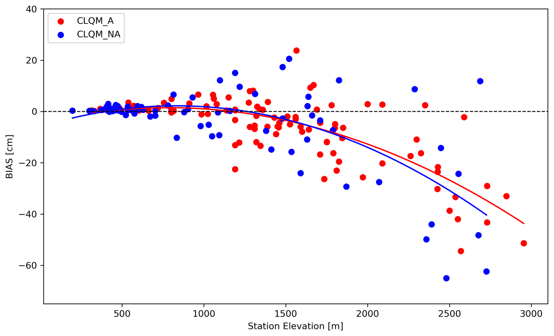
Figure 6 Bias of yearly mean snow depth [cm] vs. elevation [m] for the comparison of assimilated (red) and non-assimilated (blue) station values with respect to the OSHD-CLQM model. The curves are polynomials fits of second degree.

When looking at the entire country, i.e., grid points of all stations across Switzerland (Fig. S4), the analysis reveals a slightly better performance for OSHD-EKF, which can be best seen in the clearly smaller number of outliers and the smaller whisker range for MAAPE and R. Differences due to temporal aggregations can best be observed in RMSE, where yearly mean values are about 10 cm. This value increases to about 15 cm for monthly mean values and almost 20 cm for weekly mean values. This good performance when averaging over all grid points gives confidence in typical climatological analyses like the comparison of the annual snow depth evolution between different climate periods (e.g., 1962–1990 with 1991–2020). The corresponding plot (Fig. S6) demonstrates a clear decrease in snow depth in recent decades, which is mainly driven by less accumulation in spring and an earlier snow disappearance in summer. This finding is not new as it has been found based on station data (Klein et al., 2016; Marty et al., 2023) but can now also be demonstrated in a quantitative way with gridded data. For station data, the mentioned studies explained the snow depth decrease with higher temperatures.

3.3 Evaluation of trends

3.3.1 Elevation-dependent snow depth trends

Here, we investigate how long-term HS trends of OSHD-CLQM and OSHD-Comb compare to trends observed at stations in the different elevation bands. Figure 5 demonstrates that compared to station data, median performance scores of OSHD-CLQM and OSHD-EKF are generally (except R) very similar, demonstrating the good performance of the quantile-mapping step. However, focusing on the whiskers of the box plots, it is obvious that with OSHD-EKF smaller errors (outliers) are achieved. Therefore, using OSHD-EKF data instead of OSHD-CLQM data, when possible, i.e., OSHD-Comb, can be an asset from 1999 onward because the two datasets only differ after 1999. Any differences in their long-term trends are due to differences in the most recent period (after 1999). However, the trends of the two model chains after 1999 are still fairly similar (Fig. S5).

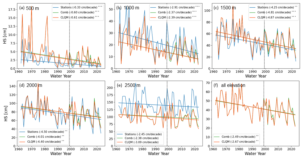
Figure 7 Trends of yearly snow depth [cm/decade] calculated using Theil–Sen slopes for the OSHD-CLQM and the combined model data series (OSHD-Comb), as well as for station measurements for the five elevation bands: (a) 500, (b) 1000, (c) 1500, (d) 2000, and (e) 2500 m, as well as (f) all of Switzerland (0–3000 m). Significance is indicated with ${}^{*}p<\mathrm{0.05}$, ${}^{**}p<\mathrm{0.01}$, and ${}^{***}p<\mathrm{0.001}$. The dashed line indicates the year 1999, before which the yearly values of OSHD-CLQM and OSHD-comb are the same.

The combined model OSHD-Comb utilizes the OSHD-EKF, which helps capture short-term variations more accurately in the period since 1999. Meanwhile, OSHD-CLQM originates from quantile mapping of the climatological model OSHD-CL onto OSHD-EKF, aiming to reduce systematic differences in the simulation of OSHD-CL (Michel et al., 2024 and Fig. 1). On the other hand, using OSHD-Comb could introduce temporal inconsistencies at the point in time when OSHD-CLQM and OSHD-EKF are combined (1998/1999; see Fig. 1), which we investigated by analyzing the involved trends shown in Fig. 7. Examining the plots in this figure reveals that the interannual variability in the modeled long-term snow depth time series (OSHD-CLQM and OSHD-Comb) agree very well, especially when comparing all elevations (Fig. 7f). But both datasets also align well with the long-term station data, particularly at elevations of 1000, 1500, 2000, and 2500 m, which demonstrates the performance of the quantile-mapping step in these elevation bands. The OSHD-Comb trend magnitude is marginally weaker than the OSHD-CLQM trend magnitude and thus closer to the station-based trend magnitude for all investigated elevations with the exception of the 2000 m band. The largest differences between station-based and model-based trends appears, again, in the lowest elevation band, which corroborates the findings of Michel et al. (2024) and Fig. 5 with large relative errors at low elevation. With a closer look at this low elevation band (Fig. 7a), we see that the largest differences occur during snow-rich winters in the first 20 years. These differences are similar when using OSHD-CL (not shown), which indicates that not the QM step but the meteorological input data and/or the temperature index model are the main reason for the large biases in the first two decades in the lowest elevation band and that the QM step fails to correct this. Focusing on the significance of the decreasing trends we see that the level of significance agrees well for all datasets and elevation bands, which is also in agreement with other studies analyzing station-based trends.

Notice that there is only one long-term station available in the 2500 m elevation band, which strongly limits the informative value of this elevation band. Therefore, an additional analysis for this elevation band has been undertaken for the shorter 24-year period of 2000–2023 (Fig. S7), where data from 14 stations are available. This figure corroborates the findings of Fig. 7e with the similarity and the nonsignificance of the trends found in this elevation band. The above results agree well with other recent studies analyzing station-based trends with mostly significant decreasing trends below about 2000 m (Matiu et al., 2021; Marty et al., 2023).

An example that demonstrates the possible differences between the two datasets OSHD-CLQM and OSHD-EKF is illustrated in Fig. 8, which shows climatological anomaly maps for the example of winter 2018 (November–April) for both datasets. The relative snow depth anomaly for this season with respect to the long-term mean (1991–2020) is clearly above average in the Alps (see high elevations in Fig. 2) and in the south for both datasets, but less consistent patterns appear at low elevations in the north. A visual comparison to the station values (marked in Fig. 8 as well) demonstrates that OSHD-EKF provides more accurate results regarding these regional differences, revealing that the Swiss Plateau experienced clearly below-average snow depth in the 2018 winter season. Moreover, OSHD-EKF in this case appears to exhibit greater spatial uniformity. This result is not surprising as Figs. 3 and 4 demonstrate that the performance of the quantile-mapping approach used in OSHD-CLQM is limited in low-snow environments (i.e., at low elevation for Switzerland).

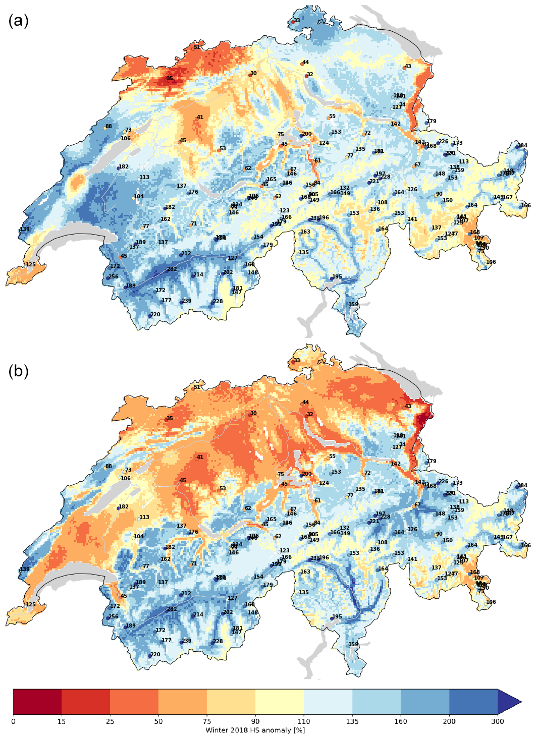
Figure 8 Relative snow depth anomaly (%) of winter 2018 (November–April) with respect to the long-term mean (1991–2020) for OSHD-CLQM (a) and OSHD-EKF (b). Red indicates below-average snow depth, yellow average snow depth, and blue above-average snow depth. The colored dots and numbers indicate station anomalies.

3.3.2 Snow depth trends at individual stations

We also conducted a trend comparison based on single grid points, since having a gridded dataset available makes it tempting to use information from single grid cells in places where no station measurements are available. We compared the Theil–Sen slopes of the yearly means of stations with those of the closest grid point from both the OSHD-CLQM and the OSHD-Comb models. The corresponding plot (Fig. 9) reveals that in the large majority of the cases the trends align well between models and stations. Moreover, there seems to be almost no performance difference between the two model chains. However, we can also observe that the bias (difference between station and model trend) is large for a small set of stations at elevations between 1200 and 2000 m. Both OSHD-CLQM and OSHD-Comb show the same eight stations that differ by more than ±4 cm/decade in their trends. Out of these eight stations, there are five stations which show a considerably weaker trend and three stations which show a stronger trend in the modeled time series compared to those of the respective stations.

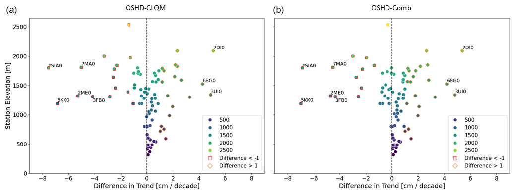
Figure 9 Scatter plots of station elevation [m] vs. the difference (station minus model) of the snow depth trend [cm/decade] for yearly values in the period 1962–2023 for OSHD-CLQM (a) and OSHD-Comb (b). Differences larger than 1 and smaller than −1 are depicted with an orange diamond and red square, respectively. Stations that show a difference greater than ±4 cm/decade are labeled.

Upon closer examination of these stations, we find that one station (7DI0) is located above the tree line, heavily wind-influenced, and subject to several relocations during the investigated period. Moreover, three stations (3UI0, 5KK0, 2ME0) are known as inhomogeneous series due to major shifts in location (Buchmann et al., 2022). These findings reveal that the new gridded datasets have some potential to find indications of potential inhomogeneities in station time series. However, there are also larger differences for four other stations, which compared to trends at neighboring stations and neighboring grid points are probably caused by station inhomogeneities (3FB0) or problems with the gridded meteorological input data (6BG0, 7MA0, SIA0). Interestingly the former three stations are all in southern regions with steep topography and only few precipitation time series available as input. These examples also indicate that when comparing station data to model values, we should sometimes use multiple grid points of a larger area for comparison instead of only one single grid cell (see Sect. 3.4 and Michel et al., 2024).

Such exceptions do not impact the informative value of the gridded trend results on a larger spatial scale. Indeed, a map illustrating the OSHD-CLQM trends for each grid point in Switzerland separately (Fig. 10) reveals significant trends at almost all low- and mid-elevation regions, which corroborates the results of Fig. 7. Elevations above 2000 m along the main Alpine ridge and in adjacent inner-Alpine dry regions show mostly nonsignificant decreasing trends, except a small area near the southwestern border (Saas Valley) with nonsignificant increasing trends. The only nonsignificant region in the lowest elevation band is located in the Rhone Valley southeast of Lake Geneva (southwestern corner of Switzerland). Moreover, Fig. 10 generally confirms the known weaker absolute trends at lower elevations (Schöner et al., 2019) by the easy visual recognizability of the Alpine valleys. Finally, Fig. 10 also demonstrates good agreement with a similar analysis, but a different model, for Austria (Olefs et al., 2020), in which partly nonsignificant trends for the Austrian region (Tirol), which is adjacent just east of southeastern Switzerland, were also found. In relative terms (Fig. S9), the trends become largest at low elevation (mainly Swiss plateau), where values between −10 % and −20 % per decade are typical. Above 1000 m, however, typical relative trends are between −5 % and −10 % per decade.

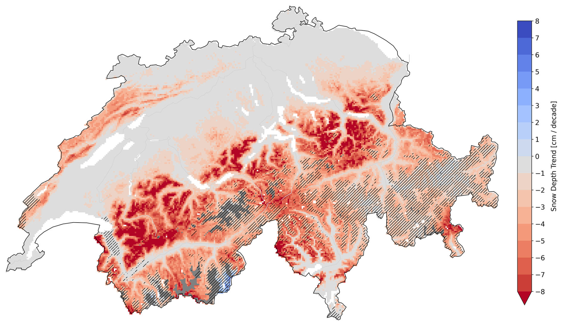
Figure 10 Trends of yearly mean snow depth (cm/decade) for the period 1962–2023 based on Theil–Sen slopes for each 1 km grid point of the OSHD-CLQM model in Switzerland. Water bodies appear white, elevations above 3000 m are colored in gray, and non-hatched areas indicate significant trends at the 95 % confidence level (p<0.05).

3.3.3 Elevation-dependent snow day trends

The number of snow cover days during a season is a useful additional metric as it reflects not only the quantity of snow in the Alps but also the duration. The duration of snow cover is important for the energy balance of the Earth's surface and holds important implications for various sectors, including ecology, winter tourism, and energy production (hydropower and PV power). Comparing the different datasets in Fig. S8 across the five elevation bands reveals that the direction of the trends (mostly decreasing) is the same in all analyses. No trend could be detected in elevation bands where the number of snow days is bounded due to our November to April season definition (low HS threshold at high elevation) or where the number of snow days was mostly zero (high HS threshold at low elevation).

There is generally less agreement in the magnitude of the trends for the number of snow cover days (Fig. S8) compared to corresponding analysis of mean snow depth (Fig. 7). Such disagreement is not uncommon, as threshold analyses in general are known for their high sensitivity, and limitations of the input data also likely contribute (see Sect. 3.4). At 500 m and with a 5 cm threshold, models predict over double the decrease compared to stations. This matches the result observed in the mean HS trend analysis at 500 m.

Having a closer look, we can see that in most instances OSHD-Comb generally demonstrates better agreement compared to the year-to-year station fluctuations. Below the elevation band of 2000 m, both models demonstrate a significant decreasing trend. At the 2000 m elevation, the models only show significance with p>0.05 at a threshold of 30 cm. However, significance is observed at all other thresholds and elevation bands up to 2500 m. The elevation-dependent pattern agrees well with that seen for snow day trends in Fig. A1 in Buchmann et al. (2023). The largest decrease in the number of snow cover days (about 9 d per decade) is found at 1000 m for the 5 cm threshold. This is likely because this elevation band coincides with the current mean snowfall limit (Scherrer et al., 2021). Below 1000 m, snow cover days are already rare, leaving little room for further decline, while above 1000 m, mean winter temperatures remain below freezing, resulting in smaller absolute decreases.

3.4 Limitations regarding input data and involved models

When utilizing the investigated gridded snow dataset for climatological analyses, the involved uncertainties of the underlying input data and methods used to derive SWE and HS should always be considered. They include the following issues.

The gridded temperature and precipitation datasets used as input for the snow model (see Sect. 2.1) are not perfectly consistent over time as the number of stations available for the spatial analysis on the 1 km grid can vary over time and elevation (Frei, 2014). It is important to keep this fact in mind when using the gridded snow datasets for trend analysis.

Furthermore, there are unresolved small-scale effects in these gridded input datasets. Regarding temperature, among these are all kinds of land cover effects (e.g., lakes and urban heat islands) and the influence of local topography. As a result, it must be expected that spatial variations are underestimated (too smooth), particularly at the scale of the grid point spacing, and small-scale patterns may not be accurately represented (in both extent and amplitude) at the scale of the model grid. This is particularly true for valley cold pools – their reproduction by the analysis critically depends on the existence of in situ measurements within these pools. Hence cold air pools may be missing completely in un-instrumented valleys (see Frei, 2014). Regarding precipitation, possible undetected station- and time-dependent measurement errors can always be an issue and the interpolation is limited by small-scale variability of precipitation. The provider of the datasets (MeteoSwiss) expects that the effective resolution of the daily gridded precipitation product is of the order of 10 to 20 km, likely even coarser in the high mountains. Additionally, measurements by rain gauges are subject to systematic errors, like gauge under-catch, which causes an underestimation of precipitation, particularly during days with snowfall and at wind-exposed locations (Yang et al., 1999). However, the problem should be, at least partially, mitigated by the QM step, which constrains the model by assimilation of snow depth observations (OSHD-EKF) and thereby indirectly also corrects for under-catch issues in the gridded precipitation dataset.

When these two gridded datasets (temperature and precipitation) are used as input for the temperature-index-based snow model, we must be aware that the temperature data represent the daily average from midnight to midnight UTC, whereas the precipitation data represent the daily average from 06:00 UTC of day D to 06:00 UTC of day D+1. This temporal mismatch is another reason for possible biases in gridded snow data, especially at shorter timescales. A particularly relevant contributing factor in this regard is the use of daily average temperatures to partition precipitation into snowfall and rain. Uncertainties arise every time a precipitation event happens at times that are colder (nights) or warmer (days) than the 24 h average temperature, which is a generic limitation of models that use input data at daily rather than hourly resolution.

Another factor contributing to the overall uncertainty is the fact that the OSHD-CLQM modeling chain is based on a temperature index model with a parameter set (Magnusson et al., 2014) that is applied over the entire six-decade-long period. This fact and the abovementioned limitations of the atmospheric input data are a reason why the assimilation of snow measurements is an important step and that the corresponding OSHD-EKF datasets are of better quality.

A further potential inhomogeneity arises when using OSHD-Comb, as two datasets of different quality are combined here. Our analysis demonstrates that the impact is small when using data for the entire country on the current time series length. But this does not need to be the case for smaller regions or shorter time periods.

Finally, it is important to keep in mind that the OSHD datasets provide SWE values, which are then converted to HS. This conversion has an RMSE of about 1.5 cm and a bias of 1 cm (Aschauer et al., 2023). Therefore, HS always has a slightly higher uncertainty than SWE.

4 Conclusions

We analyzed the potential and limitations of newly developed spatially gridded datasets of snow water equivalent and snow depth for climatological applications in Switzerland spanning six decades from 1962 to 2023. Our results demonstrate that the use of long-term gridded snow data has a high potential for climatological analysis, albeit with some limitations. Our analysis corroborates the findings of Michel et al. (2024) that the quantile-mapping approach generally achieves good results in producing long-term climatological time series of snow. In addition, we could for the first time demonstrate in a quantitative manner how the uncertainty of new gridded climatological snow depth datasets increases with shorter analysis timescales, especially for low elevations.

More specifically, a comparison of the 60+-year-long datasets to station measurements for yearly mean snow depth values revealed in general a good performance of the new gridded datasets. We also evaluated how well station-based trends were captured in the modeled gridded datasets. In general, the results demonstrated very good agreement between station- and model-based trends, i.e., clear decreasing trends for mean snow depth and the snow cover duration (based on snow days) for the different elevation bands. Yearly mean snow depth demonstrated excellent agreement with respect to the decrease per decade and the significance of this decrease for the different elevation bands, except for the lowest elevation band, where snow is generally scarce. There, the modeled trend was much stronger than the station trend. The same trend overestimation in the lowest elevation band was also found when analyzing trends of the number of snow days. However, as often with count data, the agreement between model and station trends was not as good and also depended on the threshold of the snow day definition. Generally, as shown by these results, station data are more reliable at low elevation. At higher elevations (i.e., above 1000 m a.s.l.), SPASS data (OSHD-CLQM or OSHD-EKF) from larger regions and longer periods are often preferable, as they are less location-dependent and are also available in the early and late season (early fall and late spring).

Moreover, a comparison between long-term trends of mean snow depth calculated using in situ data from individual stations and gridded data with the closest grid points revealed generally good agreement. However, for about 20 % of all stations, the disagreement between the trends was larger than 1 cm/decade and sometimes even had the opposite direction owing to either inhomogeneities in the observations or modeling/input data issues. Therefore, we generally recommend using the new SPASS datasets for trend analysis with at least some level of spatial aggregation and for elevation above 1000 m, while caution is needed for interpretation of data at the grid point level and/or in low-snow regions. Furthermore, we urge caution when using maximum values because the applied quantile-mapping method does not really capture extreme values as they are corrected according to the correction of the 99th quantile (Michel et al., 2024).

On the other hand, the generally good performance of the new datasets allows for the first time the production of, e.g., high-resolution (1 km), high-quality, country-wide SWE and snow depth maps of climatological mean values or monthly/seasonal anomaly graphs for different regions/elevations. Moreover, except for low elevations, the data provide a reliable basis to analyze elevation-dependent trends of SWE and snow depth. Hence, these datasets are an important basis for applied research in winter tourism (Troxler et al., 2025) and hydrology (Chartier-Rescan et al., 2025) in an Alpine country like Switzerland. For these reasons the two involved institutions (SLF and MeteoSwiss) use the new datasets to regularly provide maps and graphs on the current snow status in Switzerland as a climate service for the interested public or businesses (BAFU, 2024; WMO, 2024b; SLF, 2025).

Our results also reveal that it may be worth making use of the higher-quality but shorter-term OSHD-EKF dataset, which assimilates in situ snow depth data. This is especially true at low elevation and for shorter time aggregations like months or weeks. This fact also demonstrates that long-term station measurements are still indispensable, as they are needed to produce long-term, high-quality gridded snow datasets.