Spatio-temporal snow data assimilation with the ICESat-2 laser altimeter

The satellite laser altimeter ICESat-2 provides accurate surface elevation observations across the globe. With a high-resolution digital elevation model (DEM), we can use such measurements to retrieve snow depth profiles even in remote areas where snow amounts are poorly constrained. However, the adoption of these retrievals remains low since they are very sparse in space, as the satellite measures along profiles, and in time, as the revisit is 3 months. Data assimilation (DA) methods can exploit snow observations to constrain snow models and provide gap-free distributed simulations. The assimilation of observations related to snow cover is well-established, but there are currently no methods to assimilate sparse ICESat-2 snow depth profiles. We propose an approach that spatially propagates information using – instead of the classic geographical distance – an abstract distance measured in a feature space defined by a topographical index and the melt-out date climatology.

We demonstrate this framework for a small experimental catchment in the Spanish Pyrenees through three experiments. We assimilate different snow observations in an intermediate-complexity snow model: fractional snow-covered area (fSCA) retrievals from Sentinel-2, snow depth profiles from ICESat-2 located in proximity of the catchment or both fSCA and depth in a joint assimilation experiment. Results show that assimilating ICESat-2 snow depth profiles successfully updates the neighbouring unobserved catchment, improving the simulated average snow depth compared to the prior run. Another encouraging finding is that adding the snow depth profiles to fSCA observations leads to an accurate reconstruction of the snow depth spatial distribution. Evaluating the simulations with a set of independent drone-based snow depth maps using a probabilistic skill score, we find that for the accumulation season the joint assimilation's score improves by 19 % the established approach of only assimilating fSCA. The direct but incomplete snow depth information from ICESat-2 is a key constraint on simulated basin-average snow depth.

This study makes use of globally available datasets and shows the promise of adopting ICESat-2's snow depth retrievals in seasonal snow modelling, especially when also assimilating complementary observations. In light of our encouraging results, more research with different experimental designs in varying snow conditions combined with continued methodological development is desirable to further catalyse the use of these retrievals in cryospheric and hydrologic applications.

1 Introduction

Seasonal snow is a crucial element for sustaining life and an essential climate regulator (Sturm et al., 2017). It is characterized by strong spatial and temporal variability which arise from several processes such as preferential deposition, wind transport, differential radiation, turbulent heat fluxes and metamorphism (Mott et al., 2018). This is a challenge for spatially distributed modelling efforts as point measurements have a limited utility. Remote sensing thus presents a more promising method to estimate the spatial distribution of snow (Clark et al., 2011). Despite the many approaches involving satellite, airborne and drone sensors of various different types currently being used, accurately measuring the temporal and spatial variability in snow amount (i.e. mass or depth) at watershed-scale with remote sensing is still a major scientific challenge (Gascoin et al., 2024).

Since October 2018, the ICESat-2 mission measures the Earth's surface elevation through a 532 nm (green) laser along six parallel profiles (Markus et al., 2017). The geolocated photons have a centimetric vertical measurement error on flat terrain (Markus et al., 2017), while the horizontal accuracy is estimated to be between 3 and 4 m (Magruder et al., 2021). ICESat-2 data products derived from the spatial aggregation of photons over tens to a hundred metres have been used to measure snow depth by differencing with a digital elevation model (DEM) acquired during snow-free conditions. From comparison to airborne lidar snow depth observations, Enderlin et al. (2022) found that the median absolute deviation, an index of accuracy, is approximately 0.2 m for slopes < 5°, while it increases to be > 1 m for slopes > 20°. Deschamps-Berger et al. (2023) found similar results: the random error (precision) was 0.5 m for < 10° sloped terrain. Besso et al. (2024) improved the results in the same basins of the two aforementioned studies by focusing on customized data products generated with the SlideRule Earth service (Shean et al., 2023).

The ICESat-2 snow depth retrievals can quantify the snow spatial distribution at the acquisition time. However, they have limited value in directly estimating snow water resources, a trait they share with other commonly used remotely sensed observations such as fractional snow-covered area (fSCA). This limitation arises because ICESat-2 observations are only able to capture a subset of the full state of the snowpack at one to several points in time and space (Alonso-González et al., 2021; Margulis et al., 2016). In order to completely capture the spatio-temporal evolution of the snowpack, satellite observations have been used to constrain snow models with varying complexity. Herein, we focus on an intermediate complexity snow model, namely, the Flexible Snow Model (FSM2; Essery et al., 2025), which is a compromise between a detailed representation of physical processes that influence the key snow hydrological state variables and parsimonious parameterizations that allow for increased computational efficiency. The main limitation for large-scale snow modelling is the accuracy of atmospheric forcing data (Raleigh et al., 2015). This applies especially to spatially distributed set-ups where the forcing needs to be extracted from large-scale atmospheric model outputs such as coarse-resolution (30 km) global atmospheric reanalyses (e.g. ERA5; Hersbach et al., 2020).

Data assimilation (DA) offers a wealth of algorithms to fuse noisy observations with uncertain models in a Bayesian framework (Evensen et al., 2022), to obtain statistically optimal estimates together with a quantification of their uncertainty. This technique has shown considerable promise in the snow science community to meet the reconstruction and forecasting requirements needed to more accurately map the water storage services that snow provides to downstream ecosystems and communities (Girotto et al., 2020). Girotto et al. (2020) noted that most snow DA research – with a few exceptions (e.g. De Lannoy et al., 2012; Magnusson et al., 2014) – has focused on purely temporal DA where the snow in each model grid cell (or more generally spatial unit) is simulated and updated independently of its neighbouring cells and the observations therein. A greater adoption of spatio-temporal multivariate DA is recommended (De Lannoy et al., 2022). Recent studies have demonstrated the added value of spatio-temporal DA in exploiting spatially sparse snow depth observations by propagating information through covariances based on geographical distance (Cluzet et al., 2022; Cho et al., 2023). In contrast, Alonso-González et al. (2023) have shown promising results with a more general technique using a prior covariance matrix dependent on pixel proximity in a multi-dimensional space based on morphometric terrain features. However, this approach was shown only with high-resolution and high-accuracy UAV data, and has yet to be extended to emerging yet sparse space-borne snow observations such as snow depth profiles derived from the laser altimeter on board ICESat-2 (Deschamps-Berger et al., 2023; Besso et al., 2024), as recommended by comment 6 in Anonymous (2023) and by Gascoin et al. (2024).

In this study, we aim to demonstrate for the first time the value of assimilating snow depth retrieved from the satellite laser altimeter ICESat-2 in a small experimental catchment. While other studies have focused on evaluating aggregated data products from this satellite altimeter (Deschamps-Berger et al., 2023; Enderlin et al., 2022; Besso et al., 2024), we use the geolocated photon data product ATL03 (Neumann et al., 2019) with finer spatial resolution. The validation of this product is currently in progress, but preliminary results show good agreement in comparison to drone-based snow depth maps. Because of the temporal and spatial sparsity of these observations, their utility for direct mapping of snow depth along profiles via temporal DA is limited. Hence, we showcase the use of ICESat-2 data in a spatio-temporal DA scheme (Alonso-González et al., 2023) that enriches these data in that they can now be used to constrain distributed seasonal snow models for an entire catchment where the majority of grid cells are not observed by ICESat-2.

We also propose the joint assimilation of ICESat-2 snow depth and fSCA from Sentinel-2. This is compared to assimilating only ICESat-2 data or fSCA data alone, where the latter is widely available and routinely used by the snow DA community (Largeron et al., 2020). The two datasets have complementary features: ICESat-2 retrieves snow depth directly, but only along profiles; while fSCA has an indirect relationship with snow depth, but is spatially distributed. The novel scientific questions we aim to answer are:

• a.

  Can information from snow depth profiles retrieved with ICESat-2 be used to provide information about average catchment-scale snow depth and its complete spatial distribution?

• b.

  Is assimilating sparse ICESat-2 snow depth retrievals better than more commonly used fSCA observations derived from optical satellites?

• c.

  Is ensemble-based DA able to leverage information from both observation types when jointly assimilating both fSCA and sparse snow depth observations?

An important assumption of this work, shared with other high-resolution DA studies, can be outlined as follows. The snow model does not represent some of the lateral processes influencing the snowpack such as wind and gravitational redistribution: the atmospheric forcing information that is available at scale is not detailed enough to accurately capture such processes in a distributed manner. We aim to show that assimilating information from higher-resolution satellite observations can constrain the spatial distribution of snow, mitigating the effects resulting from missing the aforementioned processes that are not represented in the snow model.

2 Study area and data

The study area is the Izas experimental catchment, located in the central Spanish Pyrenees. The elevation ranges between 2075 and 2325 m above sea level and the total annual precipitation typically reaches 2000 mm, with approximately half of this in the form of snowfall as is typical for such a sub-alpine environment. Snow usually covers a large fraction of the catchment from late November to the end of May. The vegetation type is a high mountain steppe where most of the surface is covered by bunch grass (Revuelto et al., 2017).

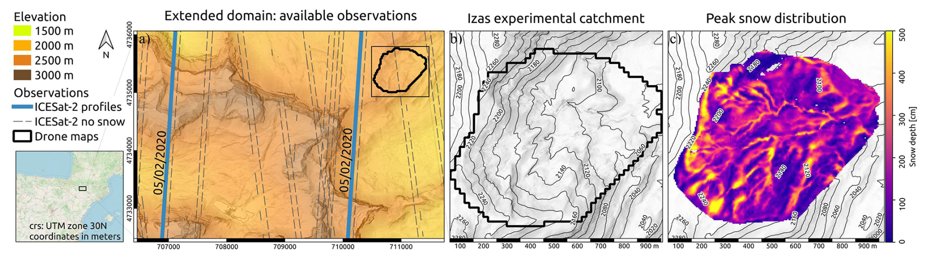
Figure 1 (a) Topography of the extended domain, located in the Pyrenees. The raw DEM data is obtained from the Centro Nacional de Información Geográfica (2025). Blue lines: ICESat-2 snow depth profiles in 2020 used in the experiments; grey dashed lines: ICESat-2 snow-free profiles that are used for coregistration purposes; black area: experimental catchment where 12 snow depth maps were acquired during the 2020 snow season. (b) The small-scale topography of the Izas experimental catchment, dictating the snow depth patterns. (c) Drone-derived snow depth map acquired on 11 March shown at the original 1 m resolution, obtained from Alonso-González (2022).

We chose this site because of the availability of several spatially distributed drone-based snow depth measurements (Alonso-González, 2022) in the 55 ha sized experimental catchment highlighted with black in Fig. 1. The drone surveys were conducted in 2020 on 14 January, 3 February, 24 February, 11 March, 29 April, 3 May, 12 May, 19 May, 26 May, 2 June, 10 June, 21 July and were already used in various DA experiments (Alonso-González et al., 2022, 2023). The original spatial resolution is 1 m, and the measurement error is assumed to have a standard deviation equal to 20 cm. Figure 1c shows the spatial distribution of snow depth close to the seasonal peak at the native resolution. Very high snow depths (>300 cm) are accumulated under the western ridgeline, in the deep valleys throughout the catchment, and at the foot of the eastern slope. Very low snow depths (<50 cm) areas are located on the southeast-facing aspects located on the northern side of the catchment as well as on the wind-blown ridges located on the southern side of the catchment.

We retrieve snow depth by subtracting the snow-off elevation obtained with a reference DEM to the snow surface elevation measured with the ATLAS instrument on board the National Aeronautics and Space Administration (NASA) satellite ICESat-2. We use the Level-2A product ATL03 (Neumann et al., 2023b), which we downloaded through the SlideRule Python client (Shean et al., 2023). This low-level product combines the time of flight data with the location of the satellite to obtain the geolocation of single photon reflection events off the snow surface. The ATLAS transmitter generates six beams arranged in three pairs, with a strong and weak beam located at a distance of 90 m, while the pairs are spaced by 3.3 km (Neumann et al., 2019). The orbit has a 92° inclination. The signal ratio between strong and weak beams is 4 to 1 and a pulse of the 532 nm laser illuminates a region (footprint) ca. 14 m in diameter. Pulses are transmitted every 1.5 ns, hence the footprints are spaced 0.7 m in the along-profile direction and have a large overlap. The expected number of photons backscattered to the ATLAS receiver for a single strong beam shot from a reflective surface such as snow ranges from seven to three depending on the slope and roughness of the surface (Neumann et al., 2019). We select two of the strong beam profiles acquired in the night of 5 February 2020, as they sample snow depth during the accumulation phase. We tested the weak beams but they were not used as those provided an observation set with fewer returns in the 20 m cell we used as unit, and a consistent vertical shift was detected. We discard the third strong beam as it is located further away at lower elevations and in forested terrain. ICESat-2's next acquisition during the 2020 snow season in the study area is in May, but the cloudy conditions weakened the surface signal and made these profiles unreliable. Most of the photon events happen on the highly reflective snow surface during the snow-covered season, but there is a relevant amount of noise due to atmospheric scattering or double bounces (Neumann et al., 2023a).

The DEM used as the snow-off reference surface is available thanks to the Spanish government's Plan Nacional de Ortofotografía Aérea (PNOA) airborne lidar initiative and its spatial resolution is 2 m. The accuracy in terms of root-mean-squared error for this lidar-based model is declared to be 20 cm in the vertical direction and 30 cm in the horizontal plane (Centro Nacional de Información Geográfica, 2025). We use snow-off ICESat-2 profiles to evaluate the vertical offset between the aforementioned DEM and the ICESat-2 acquisitions, as detailed in Sect. 3. We employ 18 profiles depicted with a grey dashed line in Fig. 1.

In addition to ICESat-2's snow depth data, we also employ snow cover information from high-resolution (∼ 10 m) multispectral satellite imagery. We used surface reflectances (the Level-2A product) obtained from the MultiSpectral Instrument (MSI) on board the Sentinel-2A and Sentinel-2B twin satellites (Drusch et al., 2012) operated by the European Space Agency as part of the Copernicus Programme. The Sentinel-2 imagery was downloaded from Google Earth Engine (Gorelick et al., 2017), which is a cloud-based platform that hosts open Earth observation data from its original source, in this case Copernicus. By manually selecting cloud-free imagery, we obtained a total of 19 scenes covering the entire study area and snowmelt season. The acquisition dates of the used scenes are shown with blue stars in Fig. 5a, and are irregularly spaced between 5 February (before peak snow) and 17 July 2022 (complete melt-out), with a median (maximum) spacing of 5 d (33 d).

3 Methods

3.1 Modelling

We simulate the snowpack at 20 m spatial resolution with FSM2 (Essery, 2015, 2023). This intermediate-complexity model represents the snowpack with up to three different layers and solves the coupled mass and energy balance equations to simulate the seasonal evolution of snow. In FSM2, seven physical processes occurring in the snowpack are represented with multiple available parameterizations. We choose the most complex representation for all the processes to obtain a more comprehensive snowpack ensemble simulation. These parameterizations are: albedo decay with elapsed time since the last significant snowfall, thermal conductivity as a function of snow density, density as a function of overburden and metamorphism, turbulent fluxes diagnosed using the Monin–Obukhov similarity theory, meltwater percolation as a function of gravitational drainage and fractional snow cover as an asymptotic function of snow depth. No lateral processes are represented in FSM2.

We drive the simulations with meteorological forcing derived from the globally available ERA5 reanalysis (Hersbach et al., 2020). Because the coarse resolution of 30 km misses the subgrid topography-driven heterogeneity of the atmospheric variables, we downscale the reanalysis with the widely used hillslope-scale topography-based downscaling tool TopoSCALE (see Filhol et al., 2023, and references therein). This process uses the pressure level data to interpolate the forcing variables to the grid cell elevation, and radiative fluxes are adjusted by taking into account local and surrounding topography as well as the position of the sun. The TopoSUB routine included in the downscaling tool allows for efficient semi-distributed spatial downscaling through topography-based clustering (Fiddes et al., 2019). We select 400 as an appropriate number of clusters to run the semi-distributed downscaling for the extended domain which has a rather small area of approximately 5 by 3 km (equal to the extent of Fig. 1a). The obtained semi-distributed forcing is then mapped back to a 20 m fully distributed grid covering the whole extended domain. This globally applicable TopoSCALE method has for example been used in similar settings to topographically downscale ERA5 reanalysis data to drive snow models both in hyper-resolution snow DA experiments (Fiddes et al., 2019) and in nationwide hillslope-scale snow simulations with FSM (Fiddes et al., 2022). The application of topographically downscaled ERA5 data to force the snow model FSM2 has already been conducted in this area in Alonso-González et al. (2022, 2023) – although another downscaling model was used. We now select the cells covering the drone maps in the Izas experimental catchment (solid black line in Fig. 1) and the grid cells in the extended domain that are intersected by the ICESat-2 tracks (blue lines in Fig. 1a), summing to a total of approximately 1900 cells where FSM2 is run.

3.2 ICESat-2 snow depth retrieval

The retrieval of snow depth observations is based on ICESat-2's accurate surface elevation measurements from individual photon reflection events. We filter such events by selecting only the ones classified as ground, as results from Besso et al. (2024) indicate such filtering improves the median absolute error. Moreover, we assign the photon events a weight based on the local neighbourhood density, using the Yet Another Photon Classifier (YAPC) algorithm. This determines the significance of individual photon events with a customized inverse-distance-weighted kNN algorithm (Sutterley and Gibbons, 2021). The neighbourhood is defined with a window length (parallel to the line of flight) of 5 m and a height of 3 m. The rationale behind this is that photons returning from the ground have a large number of neighbours as it is less likely for photons reflected from atmospheric particles or objects above the ground to be clustered together. For each approximately 4 km profile we select 60 % of the photons with the largest significance according to YAPC. In Fig. 2, the orange photons' size is proportional to their YAPC score, while the filtered-out photons are grey. Before comparing the ATL03 photon events to the snow-free reference surface elevation, it is necessary to co-register this dataset with the snow-off DEM. We employ the Nuth–Kääb algorithm to obtain the horizontal shifts using as input all the selected ICESat-2 photon events and the snow-off DEM elevations (Nuth and Kääb, 2011), implemented in the xdem Python library (xDEM contributors, 2021). Every beam is independently co-registered to account for different horizontal displacement. Individual vertical offsets (expected due to snow cover) are not removed; instead, we correct with a common offset between the DEM all snow-free ICESat-2 data following established practice (Enderlin et al., 2022; Besso et al., 2024).

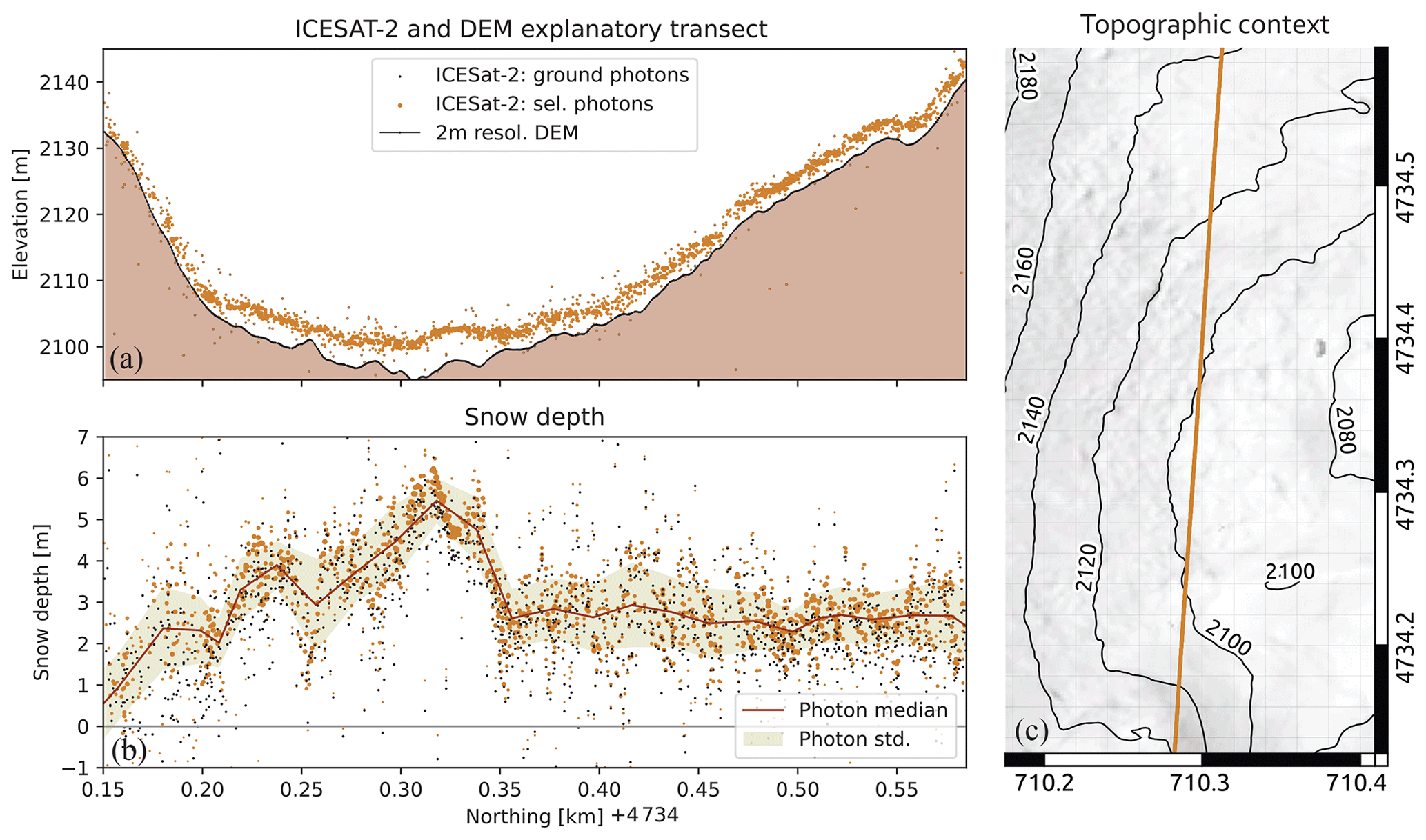
Figure 2 (a) A 400 m long segment where the photon events selected are compared with the snow-off information obtained from the 2 m resolution DEM. (b) The median operator is applied to snow depth observations from the selected photon on a 20 m moving window and the shaded area represents the 2 standard deviation range around the median. (c) The general topography of the ICESat-2 profile shown.

Snow depth is computed for each selected photon event by subtracting the elevation from the co-registered DEM. We linearly interpolate the DEM to obtain the snow-off elevation at the location of the photon event. Subsequently, we divide the snow depth observations into cells with a 20 m spatial resolution, in order to match the spatial resolution of the simulation (see Sect. 3.1). On average, 45±18 individual snow depth measurements per cell are available. Due to ICESat-2's inclined ground track (see Fig. 1a) some of the cells defined by the modelling grid have very few measurements, we hence filter out cells with less than 10 photon reflection events. In addition, the cells with an average slope greater than 40° are also filtered out, as the horizontal positioning uncertainty makes snow depth retrievals less reliable for steep terrain. In Fig. 2, a 400 m transect with a comparison between the co-registered photons and the high-resolution DEM is shown (Fig. 2a) as well as the snow depth sample distribution available along the transect (Fig. 2b). We sample the obtained snow depth distribution to retrieve an observation in each cell with the median operator. To estimate a domain-consistent statistic for the spread of the snow depth observation error, we compute the standard deviation of snow depth samples in each cell and average it over the profiles, obtaining σ_y=0.92 m.

3.3 Sentinel-2 fSCA retrieval

The fSCA retrieval algorithm is based on surface reflectances estimated from MSI on board the Sentinel-2 satellites in six bands in the visible, near-infrared and shortwave infrared. By comparing the reflectances measured in these bands to modelled spectra for snow and snow-free endmembers we infer the fSCA using spectral unmixing via a fully constrained least-squares algorithm. As shown in Aalstad et al. (2020), this approach can outperform simpler linear regression and thresholding-based approaches to fSCA retrieval, albeit at a higher computational cost. This unmixing approach to retrieving fSCA from Sentinel-2 imagery has been successfully applied both in the high-Arctic (Aalstad et al., 2020), as well as at Alpine sites (Pirk et al., 2023) in Norway. The retrievals were performed on the native 10 m grid of the visible and near-infrared reflectances from Sentinel-2, and were subsequently resampled to the 20 m spatial resolution of the simulations by averaging and subsequent inverse distance weighting. We estimate the observation error for the fSCA retrievals at 20 m resolution to be σ=0.34. Independent validation estimated the observation error σ_N at 100 m resolution to be equal to σ_N=0.07 (see Table 2 Aalstad et al., 2020). We obtained our 20 m σ estimate using the fact that the error from coarser resolutions should increase at higher resolutions according to the central limit theorem through $\mathit{\sigma }={\mathit{\sigma }}_N\sqrt{N}$, where N=25 is the number of independent 20 m cells contained in the coarser (100 m) validation.

3.4 Data assimilation

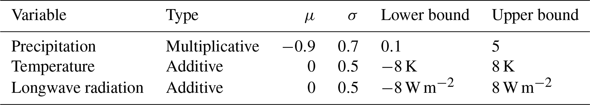
The Multiple Snow Data Assimilation System (MuSA; Alonso-González et al., 2022) allows the execution of various forms of ensemble-based snow DA. Therein, the prior distribution – a probabilistic distribution representing uncertainty over the system's state and parameter space before observations are taken into account – is represented by the spread of a finite collection of samples known as ensemble members. This spread in terms of basin-average snow depth can be seen in the grey trajectories of Fig. 5a–c. Each prior ensemble member is an FSM2 simulation obtained by perturbing a selection of forcing variables. In the presented experiments, the perturbed forcing variables are air temperature, precipitation and downwelling longwave radiation. The perturbation parameters are time-invariant throughout the water year, and are extracted from a logit-normal distribution whose prior hyperparameters are listed in Table 1. The prior perturbations are obtained by extracting samples from an associated normal distribution with mean μ and standard deviation σ. Subsequently, the inverse logit transform (sometimes called expit) with scaling is applied, resulting in a logit-normally distributed sample ranging from the lower to the upper bound (see Sect. 3.3.1 in Aalstad et al., 2018). We choose the logit-normal distribution over a log-normal or a normal distribution as the logit-normal restricts the perturbation within defined upper and lower bounds (Table 1), in contrast to other distributions which would have, respectively, only one or no bounds (Aitchison and Shen, 1980). The nature of the perturbation is multiplicative for the precipitation (in part to prevent non-physical negative values) and additive for the other variables. The negative-mean parameter of the associated normal distribution in the multiplicative perturbation parameter for the precipitation results in a right-skewed (left leaning) prior distribution with a median of 1.5.

Table 1 Hyperparameters for the extraction of the logit-normally distributed prior perturbation parameters. Numerical entries without units are implicitly dimensionless. Note that the hyperparameters μ and σ are the mean and standard deviation, respectively, of the associated normal distributions that the logit-transformed prior perturbation parameters follow.

The ensemble members representing the prior perturbation parameter distribution are updated with a deterministic version of the ensemble smoother with multiple data assimilation scheme (DES-MDA; Emerick, 2018). Such iterative `multiple DA' algorithms mitigate the negative effect of a linear forward model assumption implicit in Kalman methods (Aalstad et al., 2018; Alonso-González et al., 2022; Evensen et al., 2022). Since FSM2 is nonlinear in the mapping between atmospheric forcing and snow states, we choose four iterations, in line with the aforementioned literature. We select 40 as an appropriate number of ensemble members in order to adequately represent the prior distributions while maintaining a reasonable computational cost.

3.5 Spatial propagation of information

The key to spatially propagate information from local observations in space – that is to other simulated cells – is in the construction of the prior covariance matrix with spatial dependence (Cressie, 2011). As the spatial distribution of snow depth is strongly governed by topography, and as the relative patterns are often repeated year after year, we adopt a spatio-temporal snow DA approach based on generalized non-dimensional distances (Alonso-González et al., 2023). Details on the practical implementation and the theoretical background of this method can be found in Alonso-González et al. (2023). The key innovation of this method was to define a generalized prior correlation function dependent on the proximity of cells in a multi-dimensional feature space. Herein, we adapt the method to our novel ICESat-2 snow depth DA problem. After a careful assessment of various predictors, we select the following two features as the dimensions for the feature space:

1. CSMD: the Climatology of Snow Melt-out Date is obtained by averaging the date (day-of-water-year) when the snow melted out in a selected pixel, extracted from Sentinel-2 fSCA time series provided by the Theia land data centre (Gascoin et al., 2019). A climatology consisting of five water years was used (2017–2021). This is a new and potentially globally available feature that was not used in Alonso-González et al. (2023).

2. TPI: the topographical position index (Weiss, 2001) is computed as the difference of the cell's elevation compared with its neighbourhood defined as a 24 m radius – selected based on the results of regression experiments targeting snow depth in the Izas experimental catchment (Revuelto et al., 2014). It represents the exposure of the terrain at the mentioned scale, so that cells with negative TPI are located in a concavity or a valley and positive TPI are cells in convex terrain such as a ridge relative to its surroundings. The index is computed with the high-resolution snow-off 2 m DEM to capture small-scale topographic effects. To match the simulation resolution of 20 m, we use the average of all high-resolution TPIs within each model grid cell.

Figure 3 shows the spatial distribution of the aforementioned features at the modelled resolution (20 m) in the experimental catchment as well as the relation between snow depth and the selected coordinates.

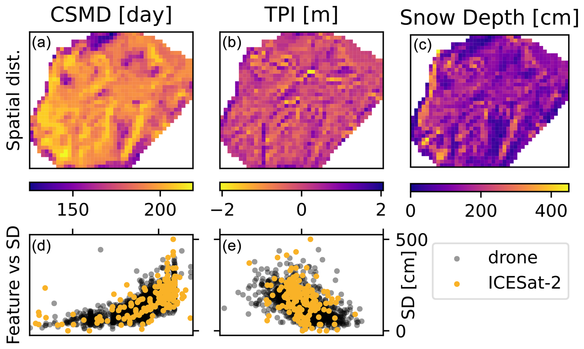
Figure 3 (a, b) Spatial distribution of the feature dimensions Climatology of Snow Melt-out Date (CSMD) and Topographical Position index (TPI) in the Izas experimental catchment. (c) Spatial distribution of snow depth derived from the drone map of 3 February. (d, e) The dimension's relation with snow depth from the drone map acquired on 3 February (black) and with ICESat-2 for the observed profiles on 5 February (yellow).

As the dimensions of the feature space have different units, each is standardized and made non-dimensional by applying a z-score, so that each set of coordinates has a zero sample mean and sample standard deviation equal to 1. Secondly, inspired by the concept of automatic relevance determination (Murphy, 2023), CSMD coordinates are increased (multiplied by 3) to make their relative weight larger as this feature correlates the most with snow depth. These operations effectively create an abstract two-dimensional feature space that we use to measure the similarity between cells using generalized distances. Figure 4 depicts both the cells in the drone domain (Fig. 4a) as well as the cells where ICESat-2 (Fig. 4b) are available in the feature space, where the coordinates are not yet standardized. The subsequent step is localization, i.e. the practice of limiting the effect of long-range spurious correlation (Sakov and Bertino, 2011). Both to define the prior correlations matrix and to perform localization we employ a widely used damping operator in the form of the Gaspari and Cohn correlation function (GC; Gaspari and Cohn, 1999), which is defined by distance in feature space and a single hyperparameter: the correlation length scale that we set to c=1.5. This operator truncates the observations located further than a radius of two times the correlation length, while including in the neighbourhood all observations located within this radius. Each cell in the neighbourhood is assigned a non-zero correlation value ρ=GC(d), computed as the GC function of the generalized distance in the feature space (as defined in Alonso-González et al., 2023). This definition of neighbourhood also leads to a reduction in computational cost through domain localization (Sakov and Bertino, 2011), whereby fewer observations are included when comparing state and observations in the update computation step of the assimilation algorithm.

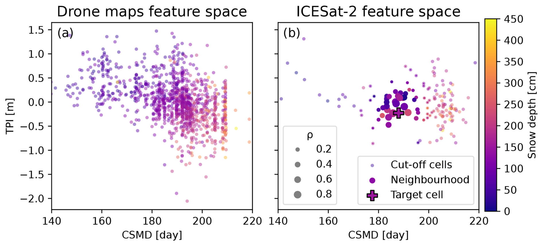
Figure 4 (a) Scatterplot depicting the position in the feature space of the cells from the drone maps. This feature space – created with TPI and CSMD – is adopted to define the similarity between cells. The points are coloured according to the snow depth observed with the drone on 5 February. (b) ICESat-2 snow depth observations in the extended catchment, displayed in feature space, with snow depth-based colouring. The cross represents one cell from the drone domain where a snow depth of 150 cm was measured. The solid points are ICESat-2 data points included in the neighbourhood for this cell, with their size proportional to the correlation ρ.

In Fig. 4b, we show one example for the definition of a neighbourhood and the assignment of the correlation value ρ to the included cells. We exemplify a situation where a cell in the catchment with drone data – depicted therein with a cross – has to be updated. The solid points in the scatterplot are included in the neighbourhood, hence information is transferred from those cells to the target cell (the cross) by means of the Kalman update (see step 11 in Algorithm 1 of Alonso-González et al., 2023), used to constrain the local forcing perturbation ensemble of the target grid cell. As cells closer in feature space to the target cell should have a larger influence, their correlation ρ is larger as can be appreciated by looking at the size of the scatter points. In simpler words, more information is transferred to the target cell from cells with large ρ compared to cells with low ρ, which are less similar in terms of TPI and CSMD. The shape of the neighbourhood is elliptic due to the differential weighting of the features, as we designed the CSMD to have a larger effect. Note that in Fig. 4 the coordinates are shown with their (non-weighted) physical dimensions.

3.6 Experiments

Three experiments are carried out where different observations are assimilated for the water year 2020. To allow a comparison where we change exclusively the assimilated variables, we use the same spatially correlated prior defined in Table 1 for all the simulations. The three experiments are designed to answer the scientific questions we presented in Sect. 1 and contextualize the value of ICESat-2 to the current standard snow DA practices:

• Snow cover experiment (C for “cover”): Temporal assimilation of local fSCA retrievals from Sentinel-2. For each grid cell, all the available local (not neighbouring) fSCA observations are assimilated. We use this as a baseline simulation.

• Snow depth experiment (D for “depth”): Spatio-temporal assimilation of neighbouring snow depth retrievals from the ICESat-2 satellite altimeter. The ICESat-2 observations of the snowpack on 5 February are assimilated. Since the profiles are located outside the experimental catchment, the information is transferred using the methods explained in Sect. 3.5 and exemplified with Fig. 4.

• Joint assimilation experiment (J for “joint”): Spatio-temporal assimilation of local fSCA and neighbouring snow depth. All the observations of experiments (C) and (D) are assimilated, and their respective observation errors are the same as for these experiments. Note that only the sparse snow depth observations are spatially propagated, while the spatially complete fSCA observations are not.

All the experiments are set up with the MuSA system (Alonso-González et al., 2023). The system was already capable of jointly assimilating different observed variables at the same location, although joint assimilation has previously only been tested in a temporal DA setting jointly assimilating fSCA and skin temperature for a single cell experiment (Alonso-González et al., 2022). Here, for the first time, we perform a hyper-resolution spatio-temporal joint assimilation of snow depth and fSCA. Each cell is updated with the local observation (if any), located in the same cell position, together with the observations in its neighbourhood defined as the set of cells located inside a search radius (d<2c) in the aforementioned feature space with dimensions TPI, and CSMD (Sect. 3.5). This domain localization step greatly reduces the computational effort, as it avoids searching through all the simulated cells. Only information from the ICESat-2 snow depth retrievals – the blue lines in Fig. 1a located in the extended catchment – is spatially propagated, as fSCA maps are available for all cells in the model domain. To allow this, we updated the MuSA system which is now able to select a subset of the available observation types to spatially propagate information. This allowed us to exclude spatially complete fSCA observations from the spatial propagation, which leads to a marked decrease in the computational cost. In practice, this implied modifying the criteria for the selection of the observations to be included in the neighbourhood. The code for the updated version of MuSA developed in this study is available online (MuSA: v2.1, Alonso-González et al., 2024).

All the experiments were executed on a local server equipped with a 1 TB memory and using approximately 40 processors. The computational time varied widely from 8 to 60 h, depending mainly on the server load and on the number of observations in a given experiment, as that number influences the amount I/O operations necessary for each update.

3.7 Evaluation

We use the 12 drone-based snow depth maps of the Izas experimental catchment (Revuelto et al., 2021) as ground truth to independently evaluate the relative performance of the DA in the three experiments. A lower bound (assuming independent errors) on the measurement error can be estimated at approximately 1 cm as we have resampled the snow depth maps to the modelling resolution (from 1 to 20 m) with the averaging operator. This is typically one order of magnitude lower than the uncertainty in the snowpack reconstruction. We aim at evaluating the sampled posterior distribution in terms of the resulting simulated snow depth goodness-of-fit to these independent observations. We evaluate our results in three ways: (i) in time, (ii) in space and in terms of snow depth distribution and (iii) for the entire spatio-temporal ensemble distribution. For (i), all the ensemble member snow depth simulations are spatially averaged over the measured experimental catchment for each day in the simulated water year, and compared to the corresponding spatially averaged drone observations. In this way, we can also evaluate how well the experiments perform in estimating the total snow volume in the catchment. For (ii), we visually compare the spatial distribution of the simulations against the drone-based map measured on the 11 March, the closest acquisition to the seasonal snow water equivalent (SWE) maximum. Since the result of the DA problem is a spatially correlated ensemble representing a statistical distribution, we show one single ensemble member simulation in order to appreciate the spatial structure embedded in the simulation. To choose the representative member, we first select the simulation state on 11 March as this is the closest drone acquisition to the peak SWE. Then we spatially average the ensembles and pick the median member of those spatial averages. Note that the selection of one ensemble member introduces an objective but casual element, as different ensemble members exhibit different spatial patterns. In the Supplement, the interested reader will find maps of the pixel-wise ensemble medians, showing a smoother spatial distribution.

To evaluate the probabilistic inference results of the three experiments (iii), we employ the continuous ranked probability score (CRPS; Hersbach, 2000), as this metric evaluates the performance of the inferred distribution represented by all the ensemble members (rather than a single point-estimate such as the median of the distribution) of each simulated cell in terms of snow depth compared to the observed reference. In particular, the CRPS quantifies both the precision (certainty or confidence) and the accuracy (ability to match the observations) of the ensemble as a whole. This is a strictly positive score, where a perfect match between the ensemble and the reference would result in a score of zero, while the larger the CRPS score the worse the result. We compute the CRPS metric for each experiment for all the available drone-based snow depth maps. To evaluate the spatial distribution of the errors we present two maps per experiment with the average score for accumulation and melting season. To evaluate how the experiment's performance varies in time we average the experiment's score throughout the measured catchment, thus receiving a single score for each drone-based snow depth map.

4 Results

4.1 Comparison with drone maps

Figure 5 summarizes the results for all the experiments and shows a comparison with the drone-based validation snow maps. We first focus on experiment (C) assimilating fSCA as a benchmark representing the current best-practice snow DA. The time series in Fig. 5a shows the prior and posterior ensemble members averaged over the Izas experimental catchment for experiment (C). The ensemble of simulations is precise (low ensemble spread) and accurate (good match to validation data) towards the end of the snow season. However, the ensemble spread is wider in the snow accumulation months and the ensemble median overestimates the catchment-average snow depth. From the map in Fig. 5d, it is discernible that the simulation correctly reconstructs the drone-observed snow depth patterns in a relative sense (comparison with Fig. 5g): the areas with larger-than-average snow depth are correctly recognized, as well as the ones with lower-than-average snow depth, despite the absolute values not being correct. Comparing the histogram in Fig. 5h with the reference in Fig. 5l highlights that the simulation average overestimates snow depth at peak SWE by 51 %. In the simulation, only 24 % of the simulated cells are inferred to have less than 150 cm of snow, while in the drone validation 46 % of them are measured in this part of the range.

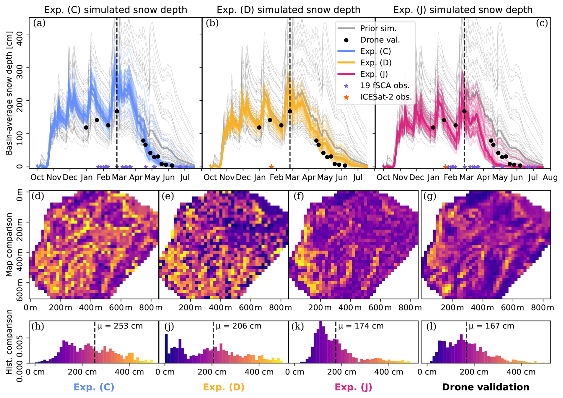
Figure 5 Panels (a), (b) and (c) show the prior (grey) and posterior ensemble simulations (coloured) as catchment-average snow depths over the whole water year for experiment (C), (D), (J), respectively. The black points are the drone-based snow map averages serving as validation data. The blue and orange stars show the timing of the fSCA and snow depth observations that are assimilated in each experiment. Panels (d), (e) and (f) show simulated snow depths are shown as maps for the 11 March 2020 (date shown with a vertical dashed line in panels above) for a representative ensemble member that is nearest to the ensemble median catchment average snow depth for experiment (C), (D), (J), respectively. (g) The corresponding 11 March 2020 drone-based snow depth map at the model's spatial resolution (20 m). The bottom panels (h), (j), (k) and (l) show snow depth histograms corresponding to the maps in the panels above, using the same colour scale. μ indicates the experimental catchment-average snow depth.

For experiment (D), Fig. 5d shows that the assimilation of the sparse snow depth profiles from a single date substantially narrows and improves the posterior distribution compared to the prior. Notably, during the winter season, the accuracy of the posterior is improved: the ensemble median and the black validation points are closer compared to (C). Also the precision is improved: the ensemble spread is narrower compared to (C). Towards the other end of the season, both accuracy and precision slightly decrease compared to the first experiment, despite still improving that of the prior simulation. Figure 5e shows that the posterior simulation is able to match many of the spatial patterns that the drone map shows in Fig. 5g, such as in the high-elevation accumulations under the ridge on the western side of the catchment. Also, patterns in the north-eastern part of the catchment are well reproduced. However, the valleys affected by wind drift and the corresponding wind-blown ridges in the south-eastern portion of the catchment are only partially reproduced. The histograms in Fig. 5j and l show the snow depth distribution comparisons. The measured catchment-average snow depth is only overestimated by 23 %. In contrast with experiment (C), low snow depth areas are well represented and better fit the histogram of the measured map. However, 25 % are simulated with very high snow depth (>300 cm), while in the drone validation only 9 % of the cells are measured with such snow depths.

For experiment (J) the time series in Fig. 5c shows that the inference produces a precise posterior ensemble (low spread) throughout the water year. In the accumulation period and up to the peak SWE, the catchment-average snow depth is accurately reconstructed. Notably, for the 11 March 2020 acquisition the measured and simulated catchment-average snow depth differ by only 7 cm. However, there is a negative bias in spring, which we do not see in experiments (C) (unbiased) or (D) (positive bias). The comparison of simulated and measured maps in Fig. 5f and g shows that the posterior simulation is able to match well most of the relative spatial patterns. For example, the accumulation below the ridge on the western border of the catchment is simulated with higher-than-average snow depth. Moreover, the absolute snow depth values are very similar in the western edge of the catchment. The cells located in the deep valleys and on the corresponding ridgelines in the south, and most of the flatter accumulation areas in the north-east have the correct relative snow depth patterns. The nearly snow-free south-east-facing slope located in the northern part of the catchment is also correctly simulated. In terms of distribution, the histograms in Fig. 5k and l show clearly that the simulation reproduces not only the mean but also the general shape of the distribution, including the tails. Low snow depths (< 150 cm), simulated for 51 % of the cells, are only slightly more than the number of cells measured in this range (46 %); as well as for very high snow accumulation values (> 300 cm): 12 % of the cells are simulated and 9 % measured.

4.2 Ensemble quantitative evaluation

Scoring the entire spatio-temporal ensemble of the three experiments allows for a more quantitative comparison of the inference performance, as Fig. 5d–f only show one representative ensemble member's simulation. Figure 6 shows the CRPS computed using the drone-based snow depth retrievals as a reference for all the available snow depth maps, focusing on the seasonal (Fig. 6a), and spatial (Fig. 6d–i) distribution. Focusing on the time evolution of catchment-average CRPS, the largest CRPS values are found during the accumulation season, while the errors decrease in the melting season, together with a reduction in the absolute values of snow depth. In the accumulation season, the average of the CRPS values show that the ICESat-2 assimilation (D) has a similar performance (44±18 cm) to the fSCA assimilation (C), whose CRPS is 44±10 cm. Both these experiments are substantially worse than the joint assimilation (J), scoring 35±7 cm. Thus, adding the ICESat-2 snow depth profiles to fSCA in the set of assimilated observations improves the overall error score by 19 % for the accumulation season. In the melting season, experiment (D) scores worst but still improves the prior CRPS by 25 %. However, experiment (C) simulations are not outperformed by the joint assimilation (J): their results are respectively 14±11 and 16±11 cm.

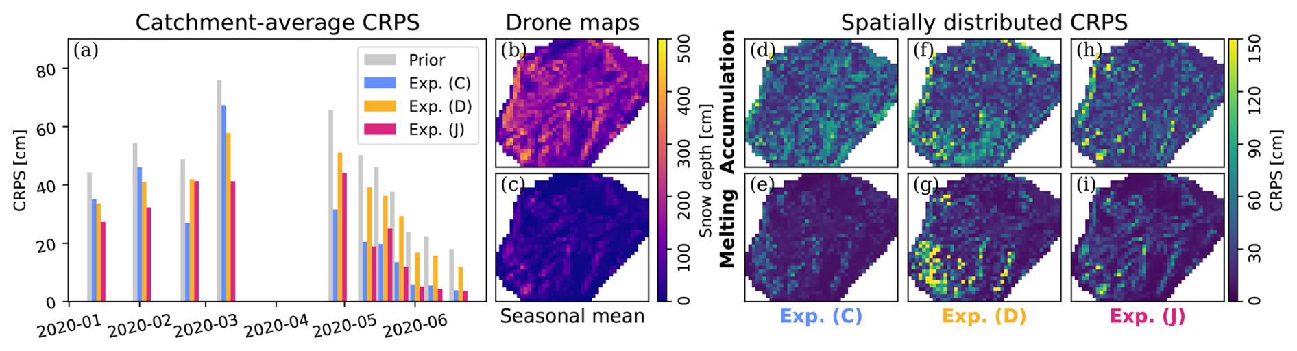
Figure 6 The performance of the three assimilation experiments is presented through the Continuous Ranked Probability Score (CRPS), where a perfect match of the compared distribution would score 0, while the larger the score the worse the result. In panel (a), the temporal evolution of the experiments' results is shown by spatially averaging throughout the experimental catchment. Panels (b) and (c) show the drone maps averaged for the accumulation (b) and melting (c) season. In panels (d)–(i), the spatial distribution of the errors obtained by averaging the CRPS computed for the validation maps acquired during the accumulation season (up to and including 11 March) is shown in the upper panels, and for the melting season in the lower panels.

Figure 6d–i shows the spatial distribution of the CRPS. For experiment (C) (Fig. 6d and e), the CRPS is generally lower for the melting season. Despite the higher values in the accumulation season, only 7 % of the evaluated cells have a high CRPS (> 100 cm). The location where large errors cluster are the windblown ridges in the south-east and on the west of the experimental catchment where a close look at Fig. 5d and g shows that medium snow depths are inferred instead of low snow depth or no snow. Experiment (D) performs better during the accumulation season: only 1 % of the cells have a very high CRPS (> 150 cm) in that season, compared to 4 % in the melting season. Such large errors are clustered in the south-west of the catchment. The low elevations on the eastern side of the catchment have better scores (compared to higher elevations) in both the accumulation and melt season. Experiment (J) shows a very similar error pattern distribution in both the accumulation and ablation season (in contrast with the other experiments). Less than 4 % of the simulated cells have a high CRPS (> 100 cm) for both the accumulation and melting season. By comparing Fig. 6h and i with the absolute snow depths (Fig. 6b and c), it is clear that the largest errors are located where very high snow accumulation are located (> 300 cm), such as the accumulation areas under the ridge on the western side of the catchment and some of the areas in the valleys in the south of the catchment. Figure S1 in the Supplement clarifies that the snow depth in the mentioned areas is underestimated.

Focusing on the use of the novel ICESat-2 snow depth retrievals, the experiments show that adding these observations for constraining the inference of the seasonal snow evolution has a positive effect on the simulation results. Comparing the CRPS over the experimental catchment of experiment (D) to the prior (no observation assimilated) shows an improvement of 20 cm for the accumulation season and 10 cm for the melting. When adding snow depth to fSCA in the set of assimilated observations – hence comparing experiments (J) and (C) – the improvement is clear with a 10 cm CRPS reduction for the accumulation part of the season. However, there is a slight increase of 2 cm in the CRPS for the melting season, despite the left-hand panel of Fig. 6 showing experiment (J)'s score being worse only for two of the drone acquisitions.

5 Discussion

In this paper, three DA experiments are carried out. All the experiments employ the same assimilation algorithm (DES-MDA), and the spatially correlated prior distributions (Table 1) are the same. In each experiment we assimilate remotely sensed observations using a different mix of snow variables, and all experiments successfully improve the prior simulation by constraining the simulations with information coming from the retrievals. However, we obtain very different results depending on the assimilated variables. The observations in the three experiments are fSCA retrieved from Sentinel-2 (C), the novel snow depth retrievals from the laser altimeter ICESat-2 (D) and finally a joint assimilation experiment using both these retrievals (J). To the best of our knowledge, this is the first example of hyper-resolution multivariate snow DA. Moreover, this is the first study not only to assimilate the ICESat-2 snow depth observations but also to show how these observations acquired along profiles located outside the area of interest can be harnessed directly through spatial propagation of information using spatio-temporal DA. This system successfully updates the snowpack states in the Izas experimental catchment both with local Sentinel-2 fSCA observations as well as ICESat-2 observations from profiles located in its proximity. The experiments with the ICESat-2 profiles exploit topographical and snow climatological indices to define a similarity measure used in the correlation function.

DA consists of combining uncertain information coming from models and observations. In our case, the unconstrained model (i.e. the prior) shows an overestimation of the snow depth, especially during the melting season (see grey simulations in Fig. 5a). The errors in the prior can be attributed to two different sources: the forcing data and the model itself (Raleigh et al., 2015). Considerable errors in the forcing data are expected to dominate and thus, by design, the forcing formulation of DA allows for the correction of such errors (Evensen et al., 2022). We emphasize that when carrying out high-resolution, spatially distributed modelling one has to expect large errors despite carefully chosen climatic forcing and topographic downscaling, given that the high spatial heterogeneity of the drivers of snow accumulation and redistribution processes cannot be explicitly represented in the forward modelling. On the modelling side, one can expect that some of the parameterized processes (e.g. albedo decay or precipitation partitioning) in FSM2 suffer from errors. Here, some of the snow processes can be substantially different and not well captured by FSM2's parameterizations, which were originally implemented for a field site in the European Alps (Essery, 2015). With the prior employed in our study (Table 1), there is just as great a need for information in the melting season as in the accumulation season. The fSCA observations contains a cumulative signal of both accumulation and melting processes. On the other hand, ICESat-2 snow depth observations from 5 February mostly contain accumulation process-related information. This could explain the better performance for the melting season of experiments (C) and (J) compared to (D) in which only observations from the accumulation season were assimilated.

5.1 Experimental results

In experiment (C), we simulate the snowpack and assimilated fSCA to create a baseline. The fSCA generally shows lower correlation with snow depth earlier in the snow season (when the ground is fully covered by snow) compared to the melting season (Girotto et al., 2020), but previous works show that assimilating fSCA can allow for an accurate reconstruction of peak SWE (e.g. Girotto et al., 2014). Indeed, experiment (C) shows high accuracy and precision especially towards the end of the season. As the experiments adopt a smoothing approach, the melt-out pattern information contained in the fSCA observations is also propagated backward in time, and the posterior simulation offers a relatively accurate reconstruction for the peak SWE: the validation is clearly close to the median ensemble spread, but the reconstruction for this part of the season is less precise compared to experiment (D), and both less precise and accurate compared to experiment (J). In terms of relative spatial patterns, experiment (J) shows the best visual agreement with the validation of drone-based maps for peak SWE, despite overestimating the absolute values in the melting season (Fig. 5).

Research question (a) asked about the value of using ICESat-2 observations to infer catchment-scale snow depth and its distribution. We can answer this question with the results of experiment (D), where we assimilate snow depth observations from ICESat-2 on two profiles outside the catchment, spatially propagating this information to the experimental catchment. The snow depth was acquired on 5 February, approximately a month before peak SWE. As Fig. 5a shows, this information leads to a more precise reconstruction of the catchment-average peak SWE compared to experiment (C), which adopted state-of-the-art methods for seasonal snow reconstruction with DA. This demonstrates that the spatial transfer of information method successfully relates snow depth and the features when averaging over the whole basin. However, not all the relative spatial patterns of the simulation match those of the validation maps (Fig. 5e and g). The observations we use in this experiment are not direct measurements in the experimental catchment, so the fact that the spatial distribution of the simulation is not entirely reproduced is not surprising. While the entire area experiences similar snow conditions there are local differences which can be only partially captured with a low-dimensional space, as TPI and CSMD do not fully characterize the snow depth distribution. For example, single cells with extreme values located in the experimental catchment might be similar in terms of TPI and CSMD to cells observed by ICESat-2 with very high snow depth, but also to some medium snow depth cells, and thus will not receive an optimal update.

Towards the end of the season, both the precision and accuracy of experiment (D) are degraded when compared to experiment (C), and the CRPS score is almost the same as for the prior for this point of the season. Here, the timing of the single assimilated observation is an important factor: most of the information of early season snow depth observations is related to accumulation processes (precipitation perturbation) rather than melting processes, in line with previous findings by Guidicelli et al. (2024). The very late melt-out date we obtain with this experiment can mostly be attributed to the fact that the prior also simulates the snowpack with such a late melt-out date. Moreover, Margulis et al. (2019) showed that assimilating snow depth observations later in the season, when some ablation processes have taken place, improves the melt season estimates compared to assimilating earlier snow depth observations. As a recommendation, we note that it would be ideal to add more ICESat-2 observations later in the water year so as to better constrain the melt season. Moreover, further experimenting with different spatio-temporal configurations for the assimilated observations in different snow environments could help shed more light on the utility of ICESat-2 in the context of seasonal snow modelling.

To research question (b), asking whether ICESat-2 snow depths or fSCA observations perform better for snow data assimilation, we cannot give a clear answer for the entirety of the snow season. We showed that assimilating ICESat-2 provides a better estimate of average snow depths during accumulation season, which is very valuable for water managers, while assimilating fSCA results in a better relative spatial distribution and melting season reconstruction.

In experiment (J), we assimilate all the observations used for the previous two experiments. These two sets of observations complement each other's coverage in time and space. ICESat-2 observations occur in February, when a deep snowpack causes fSCA relation with snow depth to saturate, and hence provides little or no instantaneous information (Margulis et al., 2015). However, fSCA is spatially complete and temporally denser which thus complements the sparse, but more direct, snow depth observations of ICESat-2, which are located along two profiles outside the experimental catchment. We show that the joint assimilation experiment (J) performs better compared to experiments (C) and (D) in terms of the CRPS in the accumulation season, showing a better representation of the spatial distribution of snow depth. For the melting season, experiment (J) has a comparable score to experiment (C), in which the melting season seems already accurately modelled. The time series in Fig. 5a and c show that in terms of catchment average snow depth, experiment (C) performs slightly better. However, Fig. 6 explains the spatial distribution of the errors and it is clear that for most of the cells both the simulations have a similar score to (C). It is only in the large snow drifts that experiment (J) is not able to simulate large snow depths. With experiment (J)'s results in mind, it is possible to answer research question (c) on whether DA is able to use information from both snow depth and fSCA combined. We found that the DES-MDA algorithm is able to jointly leverage observations of different snow variables in the same experiment, with better results compared to the independent assimilation of either observation.

5.2 Outlook and future developments

Simulating the snowpack with a physically-based model (i.e. FSM2) allows us to infer unobserved but socially relevant variables (such as SWE) or fluxes (such as snowmelt). The assimilation of fSCA has already been shown to accurately reconstruct the peak SWE (Girotto et al., 2014), and here we show that adding snow depth observations from ICESat-2 in the pool of assimilated variables improves the peak basin-average snow depth. Despite not being able to directly demonstrate it because of missing large-scale SWE validation measurements for Izas, we can postulate (based on results on SWE reconstruction experiments using complete snow depth maps Margulis et al., 2019; Ma et al., 2023) that ICESat-2-retrieved snow depth can improve the total water resource estimation for basins in complex terrain. The satellite ICESat-2 will potentially collect data until the mid-2030s, and it is necessary to further refine the methods to inform seasonal snow models and exploit this dataset for mountain water resources management. Our results show that this dataset has the potential to become a functional tool for water managers to estimate the maximum seasonal snow accumulation. However, especially within an operational snow hydrological forecasting context (e.g. Mott et al., 2023), there is a clear need to reduce the processing time of the ICESat-2 data products which currently takes months, and ICESat-2 snow depth measurements from the accumulation season may thus not be available before the end of the melt season. Moreover, the proposed method relies on a spatially correlated prior to propagate the sparse observations. This step requires the inversion of a squared matrix as large as the number of the simulated cells. Since this is a computationally expensive process, further research is recommended as approximations might be needed to extend the proposed methods to larger basins. In addition, larger domains could be split into blocks to reduce the cost of matrix inversions and thus help make this process more tractable.

In this paper, the spatial information propagation depends on a feature space defined only with two dimensions, this has not been tuned systematically to improve the results. Optimizing the selection of the feature space dimensions as well as tuning their relative weight and the correlation length scale (the hyperparameters of the spatial dependence) would be computationally expensive but may lead to better results, as experiments II and III in Alonso-González et al. (2023) show. For example, we found that the exclusion of the Winstral index (Winstral et al., 2002) from the definition of the feature space improved the inferred spatial patterns for all the experiments. We envision future work in which the optimization process could be fruitful for data-rich and vast basins such as the repeated measurements in the western US by the Airborne Snow Observatory (ASO; Painter et al., 2016). Despite the optimization or inference of the hyperparameters being foreseen to be very expensive in terms of computational resources, we acknowledge that it could be performed offline for a single season, exploiting the repeated patterns of the seasonal snow evolution (Sturm and Wagner, 2010; Revuelto et al., 2014). In terms of methods, we envision the use of hierarchical DA for the statistically optimal inference of the aforementioned hyperparameters (Katzfuss et al., 2020). In simple terms, this would increase the complexity of the DA system by defining a hyperprior on the hyperparameters that govern the spatial propagation of information. The assimilation would then lead to an optimal inference of the seasonal snow evolution for the current water year after inferring the spatial hyperparameters. Moreover, the learned hyperparameters could conceivably be transferred to other water years without the need for a second round of hierarchical inference. To alleviate computational bottlenecks, hyperparameter inference could be achieved using simpler snow models that are available in MuSA. Moreover, another option is splitting the spatial propagation problem from the temporal DA – provided that several years of snow depth maps are available for training and testing independently the hyperparameters – to alleviate the computational cost by avoiding the need to run a snow model for hyperparameter tuning. A feature space including various terrain parameters and geographical, elevation, land-use-related coordinates to define the similarity in terms of snow depth or SWE has been adopted in several recent statistical snow modelling studies based on satellite or airborne data covering larger domains (Guidicelli et al., 2024; Hultstrand et al., 2022; Liu et al., 2025).

A final note is warranted concerning the spatial resolution of the experiments (20 m). We selected this cell size to test the ability to retrieve snow depth at a hill-slope scale with the photon-counting technology that ICESat-2's ATLAS is equipped with. In experiment (D), we partially reproduced the spatial patterns observed through the drone maps. Lowering the spatial resolutions of the simulation would still be adequate for mapping water resources and would make the assimilation exercise much easier: many of the accumulation features are averaged out already at 100 m resolution. Assimilation of snow depth data at lower spatial resolution has been found to give better results in previous synthetic ICESat-2 observations propagation with neural networks (Guidicelli et al., 2024).

6 Conclusions

In this study, we present a novel approach where ICESat-2 snow depth observations along profiles are assimilated for the first time to constrain high-resolution snowpack simulations across an entire unobserved catchment. We worked with the DA system MuSA, which had capabilities to propagate information in space and time, as developed in Alonso-González et al. (2023). However, we modified it to exploit ICESat-2's sparse observations and jointly assimilate a spatially complete variable. We performed a set of three experiments where only Sentinel-2 fSCA, only ICESat-2 snow depth, and both these observations together, were assimilated while keeping the assimilation algorithm and the prior information the same, in order to evaluate the potential of the satellite laser altimeter ICESat-2 for updating seasonal snow models.

We find that including two snow depth profiles in the set of assimilated observations improves the snowpack simulation in terms of average snow depth, especially during the accumulation phase of the season – even though the snow depth profiles were located completely outside the experimental catchment of Izas (55 ha), where we validate the experiments using drone-based snow depth maps. Results show that the relative spatial patterns can partially match the validation drone maps when assimilating exclusively the snow depth profiles, since the snow depth pattern is very sensitive to the design of the spatially correlated prior which governs the spatial propagation of information. Nevertheless, the joint assimilation of Sentinel-2 fSCA and snow depth from ICESat-2 bridged such limitations and performed best in terms of average snow depth as well as capturing the spatial distribution.

These findings indicate that the ICESat-2 satellite can be exploited to improve the current state-of-the-art snow reanalyses generated by assimilating fSCA. Notably, the proposed workflow exploits globally available datasets. Provided a high-resolution DEM – which the geosciences community generally advocates the need for – ICESat-2's surface elevation measurements can be used to observe snow depth along profiles in inaccessible regions where snow amounts are still very hard to quantify. As multivariate DA techniques mature, the snow community can begin to exploit the plethora of snow observations (e.g. snow depth, fSCA, or land surface temperature) to constrain snow models and to shed light on the still unsolved snow hydrology problem of inferring the spatial and temporal distribution of SWE.