Assimilation of L-band interferometric synthetic aperture radar (InSAR) snow depth retrievals for improved snowpack quantification

The integration of snow hydrology models and remote sensing observations via data assimilation is a promising method to capture the dynamics of seasonal snowpacks at a high spatial resolution and to reduce uncertainty with respect to snow water resources. In this study, we employ an interferometric synthetic aperture radar (InSAR) technique to quantify snow depth change using modeled snow density and assimilate the referenced and calibrated retrievals into the Multilayer Snow Hydrology Model (MSHM). Although the impact of assimilating snow depth change is local in space and time, the impact on snowpack mass properties (snow depth or snow water equivalent, SWE) is cumulative, and the InSAR retrievals are valuable to improve snowpack simulation and to capture the spatial and temporal variability in snow depth or SWE. Details on the estimation algorithm of InSAR snow depth or SWE changes, referencing, and calibration prove to be important to minimize errors during data assimilation.

1 Introduction

Remote sensing and distributed modeling of snowpack with data assimilation are promising methodologies to quantify snow water resources (including its condition) and to reduce uncertainty. Current and upcoming snow remote sensing using synthetic aperture radar (SAR) aims to provide global coverage at a hyper-resolution, which is needed to quantify snow variability with reduced uncertainty. Recent studies have mostly used either backscatter approaches (Lievens et al., 2019, 2022; Singh et al., 2024; Tsang et al., 2021) or interferometric SAR (InSAR) techniques (Guneriussen et al., 2001) to quantify snow depth and snow water equivalent (SWE). The latter has been applied extensively for SWE retrievals from dry snowpacks using ground-based (e.g., Leinss et al., 2015; Ruiz et al., 2022) and satellite-based SARs (e.g., Conde et al., 2019; Dagurov et al., 2020; Deeb et al., 2011; Guneriussen et al., 2001; Lei et al., 2023; Li et al., 2016; Li and Sturm, 2002; Liu et al., 2017). The InSAR technique assumes that the volume backscatter and absorption of microwave signal in the snowpack are negligible, with the backscatter at the ground–snowpack interface being dominant while the slow propagation of radar waves through snowpack (depending on the dielectric property) results in phase delay. Previous studies have also shown that the InSAR retrievals are more suitable at longer wavelengths (e.g., L-band) owing to the transparency of dry snow and forest over snow, the preservation of coherence for longer periods of time, and the larger thresholds for phase wrapping. With the upcoming NASA–ISRO (Indian Space Research Organization) SAR (NISAR) mission, multiple studies with airborne L-band UAVSAR (uninhabited aerial vehicle synthetic aperture radar) data from the 2020 NASA SnowEx campaign have already demonstrated the potential of InSAR for snow remote sensing (e.g., Bonnell et al., 2024; Marshall et al., 2021; Hoppinen et al., 2023; Idowu and Marshall, 2022; Marshall et al., 2021; Palomaki and Sproles, 2023; Tarricone et al., 2022).

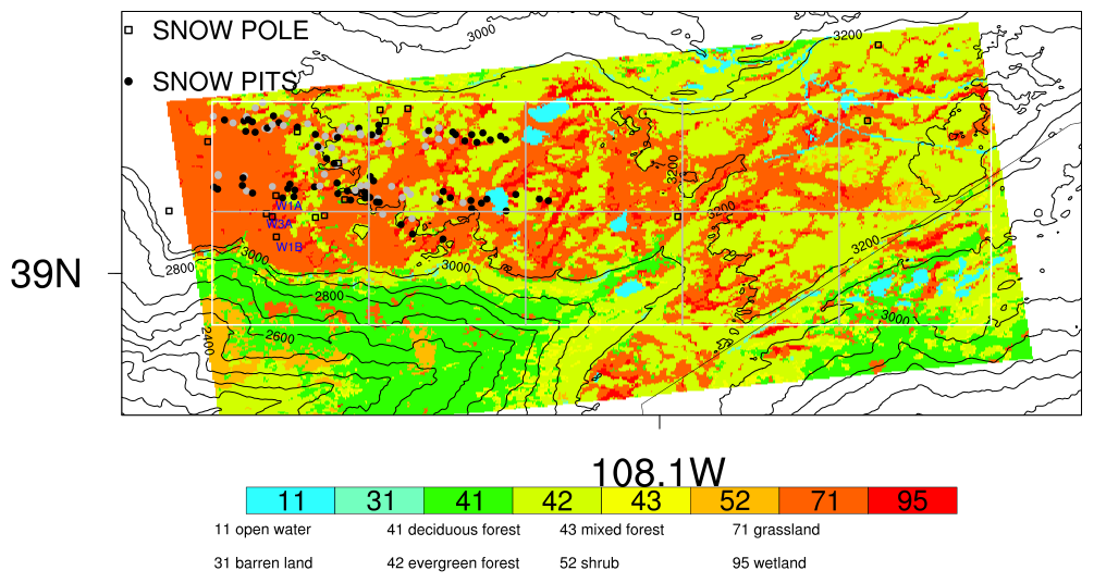
Figure 1 The spatial pattern of land cover and topography over the Grand Mesa (GM) domain (white outline). The gray boxes outline the 3 km atmospheric grids. The solid-black/solid-gray circular and square markers show the locations of snow pit and snow pole measurements available from the SnowEx'20 campaign. The snow pole measurements used for calibration of InSAR retrievals are also highlighted with their names.

InSAR retrieval algorithms need spatial data of snow density and referencing to estimate the spatial variability in absolute snow depth or snow water equivalent (SWE). Leinss et al. (2015) have proposed a modified InSAR technique to circumvent the need for snow density in SWE retrievals by introducing an additional parameter with very small variability for a range of incidence angles and snow densities; their approach also assumes that the vertical profile of snow density does not change between the two dates for each InSAR pair. However, the density profiles can change depending on the time interval between revisits, new snowfall events and weather conditions that may impact the top layer of the snowpack. Furthermore, snow density might still be needed when referencing the retrievals to obtain absolute snow depth or SWE for assimilation purposes. Hyper-resolution snow hydrology models driven by realistic hydrometeorological forcing can potentially provide a good estimate for the InSAR algorithm, and in turn, the assimilation of InSAR retrievals can potentially improve the modeled snowpack states. Earlier studies have already shown the potential for assimilating the retrieval of snow depth or SWE from airborne or satellite SAR to improve modeled snowpack and reduce uncertainty (e.g., Girotto et al., 2024; Pflug et al., 2024; Shrestha and Barros, 2025a). The upcoming launch of the NISAR mission that will provide L-band measurements globally provides an impetus to investigate the assimilation of InSAR retrievals and the associated uncertainty quantification, with potential application to operational water prediction. Here, we leverage the multiple in situ and airborne snow measurements available from NASA's SnowEx'20 (Marshall et al., 2019) campaign over Grand Mesa to (1) evaluate L-band InSAR retrievals of snow depth and (2) assimilate the retrievals into a distributed snow hydrology model to evaluate the impact on the simulated macro-physical snow properties and their uncertainties. We evaluate the L-band InSAR retrievals at their native resolution over different snow depths and types of land cover against ground-based measurements and airborne lidar (light detection and ranging) retrievals. While the InSAR retrievals only provide a change in snow depth, data assimilation requires total snow depth. Therefore, we use the airborne lidar measurements of snow depth to reference the InSAR retrievals and obtain the total snow depth. The InSAR retrievals with the first flight date (but different repeat passes) in common with airborne lidar measurements of snow depth were used for assimilation during different time windows, and the other InSAR retrievals were used to evaluate the ensemble snow hydrology model prediction of snow properties and to characterize the impact of assimilating the InSAR retrievals of snow depth.

2 Methods

2.1 Study area

The study area is located over the western part of Grand Mesa Plateau, Colorado, USA (GM domain; Fig. 1). The land cover is dominated by grassland and mixed forests across the plateau, with elevations ranging from 3000 to 3200 m. There are several scattered open water bodies (e.g., lakes and reservoirs), as well as areas with shrubs and wetlands. During the SnowEx'20 campaign, Grand Mesa hosted an intensive-observation period (IOP) during the snow-on season, including bi-weekly UAVSAR flights and airborne lidar data collection.

2.2 Data

2.2.1 UAVSAR

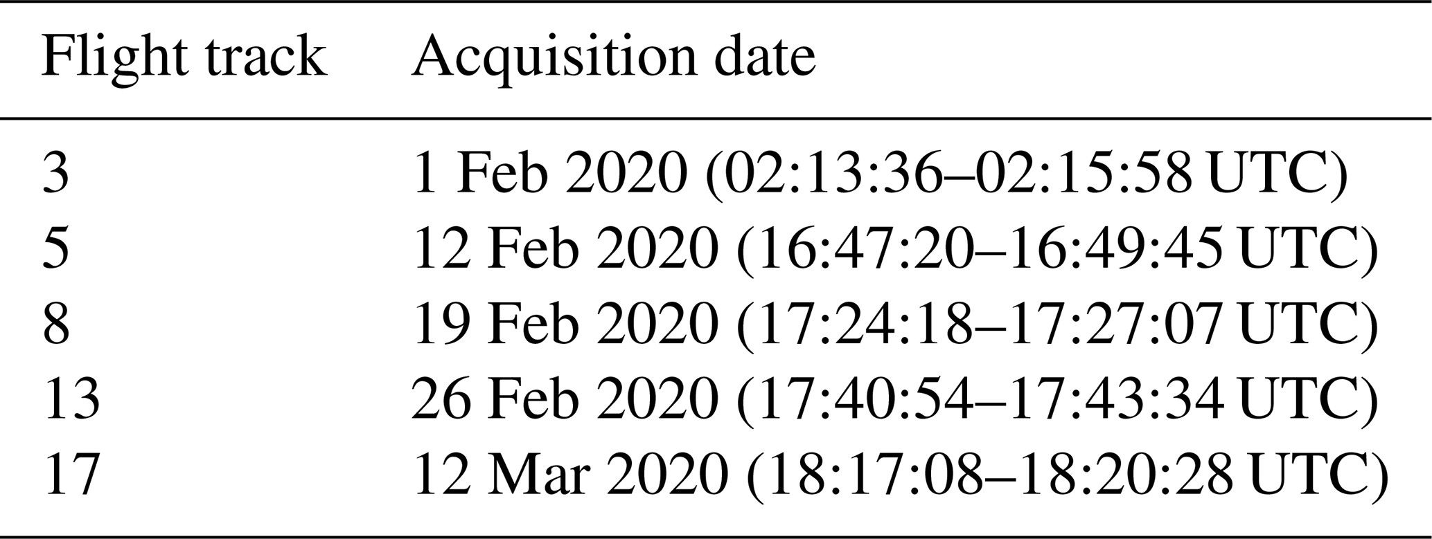
UAVSAR is a fully polarimetric L-band synthetic aperture radar designed to obtain high-quality airborne repeat pass interferometry (Hensley et al., 2008; Rosen et al., 2006). The radar operates at a frequency of 1.26 GHz (λ = 0.2379 m) with a bandwidth of 80 MHz and is mounted on the NASA Gulfstream III, flying at a nominal altitude of 13 800 m. UAVSAR data are available from the ASF-DAAC for multiple campaigns (https://api.daac.asf.alaska.edu/services/utils/mission_list, last access: 10 August 2024). The uavsar_pytools script (Keskinen et al., 2022; https://github.com/SnowEx/uavsar_pytools, last access: 10 July 2024) was used to download and convert InSAR georeferenced binary grid files to GeoTIFF in WGS84 for Grand Mesa (SnowEx'20). The interferometric data consist of the interferogram, coherence and unwrapped phase in quad polarizations, including the digital elevation and incidence angles along the flight path. In some cases, all polarizations were not available. There were seven InSAR pairs available based on five UAVSAR flights for repeated flight paths at a heading of 274° (Table 1). The flight maps are available from https://uavsar.jpl.nasa.gov/cgi-bin/data.pl (last access: 25 February 2025). The interval between the InSAR pairs varied between 7 and 40 d (e.g., track 3–5 (11 d), 3–8 (18 d), 3–13 (25 d), 3–17 (40 d), 5–8 (7 d), 8–13 (7 d) and 13–17 (15 d)).

Table 1 UAVSAR flight retrieval dates for Grand Mesa during the SnowEx'20 campaign.

2.2.2 Snow pit and snow pole measurements

The snow pit data include measurements of snow temperature, snow depth, snow density, snow stratigraphy, snow grain size, liquid water content and snow water equivalent over Grand Mesa. The SNEX20_GM_SP collection (Vuyovich et al., 2021) has 154 snow pit measurements between 27 January and 12 February 2020. Similarly, the SNEX20_TS_SP collection (Mason et al., 2024) has time series of snow pit measurements between October 2019 and May 2020 obtained by the SnowEx community during the 2020 campaign.

The snow pole data (SNEX20_SD_TLI) consist of snow depth measurements based on time lapse imagery that captures a snow pole in each image (Breen et al., 2022). The temporal coverage for these data is from 29 September 2019 to 10 June 2020. The cameras took images either three times a day (11 AM, 12 PM, 1 PM; all times are mountain standard time) or twice a day (11 AM and 12 PM). The cameras were placed in nine different environments over the Grand Mesa based on a tree density map (treeless, sparse and dense) and snow depth (shallow, intermediate and deep). The snow depth classification was based on Airborne Snow Observatory (ASO) lidar retrievals from 8 February 2017. The error estimates for each camera vary and range from ± 2 to ± 16 cm. More details are also available from https://snow.nasa.gov/sites/default/files/users/user354/SNEX-Campaigns/2020/NASASnowEx20_ExperimentPlan_v15.pdf (last access: 25 February 2025).

2.2.3 ASO

The Airborne Snow Observatory (ASO; Painter et al., 2016) lidar-derived snow depths at a 3 and 50 m resolution for Grand Mesa are available for 1 and 2 February (together) and 13 February during the SnowEx'20 campaign. The snow depths over forested area represent snow depths at the ground. SWE estimates were also available from ASO at a 50 m resolution based on bias-corrected snow density using a snow hydrology model with a 50 m resolution. The reported uncertainty in the data was 5.8 and 1.7 cm at a 3 m resolution for the two dates and less than 1 cm at a 50 m resolution for both dates. In the ASO retrievals for SWE, the snow density was obtained by calibrating the modeled density with ground-based observations.

2.2.4 Atmospheric data

The High-Resolution Rapid Refresh (HRRR; Dowell et al., 2022) 3 km first-hour forecast data for water year 2020 were downloaded using a Python package (Blaylock, 2024; https://doi.org/10.5281/zenodo.4567540). The HRRR ensemble consists of 36 members for data assimilation (DA) and 9 members for the forecast run but were not available on the servers except for the single forecast. These HRRR data were used to estimate atmospheric correction of the InSAR phase and were used as offline atmospheric forcing for the snow hydrology model. The HRRR grids interpolated to regular geographic grids are also shown over the GM domain (Fig. 1).

2.3 InSAR snow depth retrieval

The total interferometric phase difference obtained with repeat pass SAR data over a snow-covered region includes contributions due to phase impacts from flat Earth, local topography, atmospheric delay, snowpack, and random and systematic errors. While the random error mostly comes from the temporal decorrelation, assuming that phase impacts from flat Earth, local topography and systematic errors are accounted for in the UAVSAR InSAR processing chain, the extraction of the phase contribution only requires accurate estimation of the phase contribution due to atmospheric delay (see Appendix A). With a known InSAR phase difference (Δ∅_s) due to the presence of snowpack, the change in snow depth (Δz_s) can be estimated following Guneriussen et al. (2001) for coherent reflections:

$$\begin{array}{}\text{(1)}& \mathrm{\Delta }{z}_{\mathrm{s}}=-\left({\displaystyle \frac{\mathit{\lambda }}{\mathrm{4}\mathit{\pi }}}\right){\displaystyle \frac{\mathrm{\Delta }{\mathrm{\varnothing }}_{\mathrm{s}}}{\left(\text{cos}{\mathit{\theta }}_i-\sqrt{\mathit{\epsilon }-{\text{sin}}^{\mathrm{2}}{\mathit{\theta }}_i}\right)}},\end{array}$$

where λ is the SAR wavelength, θ_i is the incidence angle and ε is the bulk snowpack permittivity. For dry snow, ε^′′ is negligible compared to ε^′, and the relationship between snow density ρ_s [kg m⁻³] and permittivity can be expressed according to Matzler (1996) and Wiesmann and Mätzler (1999) as follows:

$$\begin{array}{}\text{(2)}& \mathit{\epsilon }=\mathrm{1}+\mathrm{1.6}\times {\mathrm{10}}^{-\mathrm{3}}{\mathit{\rho }}_{\mathrm{s}}+\mathrm{1.8}\times {\mathrm{10}}^{-\mathrm{9}}{\mathit{\rho }}_{\mathrm{s}}^{\mathrm{3}}.\end{array}$$

Field measurements of density data are generally sparse and may not be available for all the periods. Also, for future NISAR mission, field measurements alone will not be able to provide the snow density for all grid locations. So, we use modeled snow density (the Multilayer Snow Hydrology Model (MSHM) reference run) driven by atmospheric forcing from an operational numerical weather prediction (NWP), which can be applied everywhere to obtain the bulk snowpack permittivity.

Interferometric coherence is important to assess the uncertainty in the retrievals of snow depth, as the retrieval errors increase with decreases in coherence. Ruiz et al. (2022) used a ground-based 1–10 GHz SAR system with InSAR capabilities to examine the environmental impact on observed coherence for snow-covered surfaces. For example, increases in air temperature leading to snowmelt are associated with large drops in snow coherence besides wind, with precipitation and with large changes in temperature gradients. Compared to the X-, C- and S-bands, L-band measurements exhibit higher coherence over longer temporal baselines and smaller errors in SWE retrieval, indicating better suitability for InSAR applications.

The estimation of Δz_s following Eq. (1) assumes that the density of the snowpack is uniform with depth and that the underlying profile does not change with time. The latter assumption is problematic, as the snow density of the underlying profile could change due to physical processes (e.g., compaction) depending on the temporal baseline of the repeat pass and fresh snow. Besides, natural snowpacks are characterized by multilayer vertical stratigraphy with varying snow densities, and the phase delay is an integral of the phase delay over the multiple layers (Leinss et al., 2015). Using $\mathrm{\Delta }\text{SWE}={\sum }_{j=\mathrm{1}}^N\mathrm{\Delta }{z}_{\mathrm{s},j}{\mathit{\rho }}_{\mathrm{s}},j/{\mathit{\rho }}_{\mathrm{w}}$, where ρ_w is the density of water and $i=\mathrm{1},N$ are the multiple layers, Leinss et al. (2015) proposed a linear relationship between InSAR phase change and SWE change as follows:

$$\begin{array}{}\text{(3)}& \mathrm{\Delta }\text{SWE}=-\mathrm{\Delta }{\mathrm{\varnothing }}_{\mathrm{s}}\left({\displaystyle \frac{\mathit{\lambda }}{\mathrm{2}\mathit{\pi }\mathit{\alpha }}}\right){\left(\mathrm{1.59}+{\mathit{\theta }}_i^{\frac{\mathrm{5}}{\mathrm{2}}}\right)}^{-\mathrm{1}},\end{array}$$

where α is an optimal correction factor ranging from 0.92 to 1.07 for a wide range of incidence angles (up to 65°) and snow densities (up to 900 kg m⁻³). With this formulation and using an optimal α, they estimated a maximum error of 10 %. To reduce the uncertainty in snow density, the above method could be directly used to estimate changes in SWE. However, errors due to variations in the density profile tied to the temporal baseline between the repeat passes still need to be addressed.

Since we evaluate the model results using snow depth measurements from the lidar and ground-based measurements, we employ Eq. (1) for the estimation of snow depth change in this study. Earlier studies (e.g., Bonnell et al., 2024; Marshall et al., 2021; Palomaki and Sproles, 2023) have also used the same approach. Also, InSAR retrievals only provide changes in snow depth or SWE, so even for SWE changes, one would require prior SWE measurements or snow depth and snow density to obtain absolute SWE for assimilation. In general, snow depth measurements are more readily available (e.g., lidar or ground measurements), and models with data assimilation can provide a close estimate of snow density, so this study also provides a framework for using InSAR snow depth change for data assimilation. Using the atmospherically corrected unwrapped-phase images from the UAVSAR data, the snow depth was retrieved over the GM domain in the native grid resolution (approx. 5 m) using average bulk snow density between two repeat pass dates from MSHM reference runs. Note that the estimated change in snow depth is also well below the limit for a possible phase wrapping effect in the L-band, which is around 69 cm for λ = 23.6 cm, θ_i = 23° and ρ_s = 300 kg m⁻³ (Deeb et al., 2011). Here, it is also important to note that the estimated change in snow depth is a relative change, and without a snow-free scene or a known point change in snow depth, it is not possible to relate the relative change in snow depth to the absolute snow depth change. Previous studies (e.g., Bonnell et al., 2024; Conde et al., 2019; Hoppinen et al., 2023; Palomaki and Sproles, 2023; Tarricone et al., 2022) have used different methods (e.g., finding pixels with no changes or using pixels with known changes) to calibrate the InSAR retrievals to obtain the absolute change in snow depth or SWE. In this study, we use the snow pole measurements over grasslands for the calibration. For cases, where the measurements cannot be collocated due to missing retrievals, we use the snow pole measurement over the sparsely forested areas. In addition, we use an average over a 3 × 3 square box in the UAVSAR scene to reduce any uncertainty due to the GPS location of snow pole measurements. The InSAR snow depth change for a 3 × 3 square box (native resolution) was compared to snow pole measurements from a treeless environment (W1A, W1B and W3A, linearly interpolated to the time of the repeat pass flight) for calibration, and the average value was used for the calibration. For 1–12 February retrievals in HV and VH polarization (which had a large quantity of missing data), snow pole measurements from W5A, W6B and W6C were used for calibration. Further, we use VV polarization with higher coherence for spatial evaluation with lidar data, but since it was not available for all retrievals and since HH polarization also exhibits higher coherence and similar results to VV polarization, HH is used for the InSAR retrievals and data assimilation.

2.4 MPDAF and experiment setup

The Multi-Physics Data Assimilation Platform (MPDAF v1.0; Shrestha and Barros, 2025a) employs a coupled framework of the Multilayer Snow Hydrology Model (MSHM v3.0; Cao and Barros, 2020; Kang and Barros, 2011b, a; Shrestha and Barros, 2025a) and the NCAR Data Assimilation Research Testbed (DART; Anderson et al., 2009; NCAR DART Team, 2023). MSHM is a distributed 1D-column model that solves the mass and energy budgets of the snowpack. Key physical processes of snow hydrology – snow/rain partitioning, snow accumulation, compaction, melting and melt–runoff including snow microstructure evolution – are well represented in the model to simulate the macroscopic and microscopic snow properties. The snow microstructure evolution is simulated using a detailed microphysical scheme based on the CROCUS snowpack model (Vionnet et al., 2012). The bottom-boundary conditions are kept constant during the cold season, assuming frozen soils for snow-on conditions and fixed deep-soil temperature. Fresh-snow density in this study is based on the parameterization of Hedstrom and Pomeroy (1998), and wet-bulb temperature is used as the threshold to partition precipitation into rain or snow (Wang et al., 2019). Currently, the rain versus snow partitioning only allows for existence of rain or snow and does not allow for mixed forms of rain/snow. More details about the parameterizations can be inferred from the studies mentioned above. Following Cao and Barros (2020), the snow albedo is provided externally using the NLDAS Mosaic Land Surface Model L4 v2.0 albedo data (Xia et al., 2012a, b).

In DART, we use the ensemble adjustment Kalman filter (EAKF; Anderson, 2003) with enhanced spatially varying state space inflation (Anderson, 2009; El Gharamti, 2018). Assimilation is carried out using observed integrated quantities like total SWE or total snow depth, and the increments are then distributed vertically to the model states (snow depth, snow density and SWE) using a repartition algorithm (Shrestha and Barros, 2025a).

For ensemble Kalman filters, ensemble sizes of fewer than 20–30 can lead to statistical errors, and larger ensemble sizes take longer to run with very little benefit. So, an ensemble size of 30–100 is recommended for use with ensemble Kalman filters in DART. In this study, we have only two DART state vectors and use 48 ensemble members, which is also constrained by the computational and data storage requirements for hyper-resolution runs. In MSHM, vertically discretized snow depth and SWE are prognostic variables. However, we only use the integrated quantities of these prognostic variables (i.e., total SWE and total snow depth) as state vectors in DART, which are updated by the ensemble filters (e.g., EAKF, as is used here). The ensemble filter assumes a Gaussian relation between the variables in the joint state space prior distribution. First, update increments are computed for each ensemble sample of the observation variable, which is then used to solve for the increments for each state variable. This requires prior cross-covariance of each state variable with observation variables, along with the variance of the observation variable (see Anderson, 2003, for details). Then, we use a newly developed repartition algorithm to distribute the increments in the vertical profile with mass conservation (snow density is updated). For bulk or single-layer snow hydrology models, such repartitioning is not needed. DA directly impacts the top layers of the snowpack where snow is added or removed based on assimilation increments. The lower layers are only impacted by the modeled snow evolution after the assimilation, primarily due to the addition of new layers on top or the removal of existing snow layers. The localization setups were used such that the observations only impact the model grid points where they are located. The goal is to reduce the impact to the surrounding grids with different land cover characteristics and, therefore, different retrieval uncertainties, such as in the case of forested and non-forested grid points. Thus, the cutoff radius that determines the region of spatial impact of the assimilated variable was set to approximately 100 m (close to the model resolution).

The snow hydrology model is set up over the GM domain using an approximately 90 m resolution with 66 × 165 grid points. The maximum number of snow layers in the model was set to 30. The merged atmospheric forcing data are also interpolated to a regular geographic grid and disaggregated to a 90 m resolution. Here, no downscaling algorithms are applied to the forcing data, and the disaggregation technique applies homogeneous forcing over the subgrid pixels – this also allows us to highlight the impact of hyper-resolution data assimilation. Further, scaling analysis of SAR backscatter and lidar snow depth estimates in mountainous regions including Grand Mesa (Manickam and Barros, 2020; Mendoza et al., 2020b, a) shows that a minimum variance is reached at scales of 100–250 m, with clear scaling breaks tied to very high variance at very small scales and to topography and land cover at larger scales. The spatial resolution of this study is around the scale of minimum variance.

The MSHM reference run (CTRL) was integrated from 1 October 2019 to 1 April 2020 using the default HRRR forcing data. For data assimilation (DA) runs, 48 ensemble members were generated by perturbing the model forcing data. The precipitation is perturbed using multiplicative noise drawn from a uniform distribution U[−0.4, 0.4]. The incoming shortwave and longwave radiation are also perturbed using multiplicative noise from a uniform distributions U[−0.05, 0.05] and U[−0.1, 0.1], respectively.

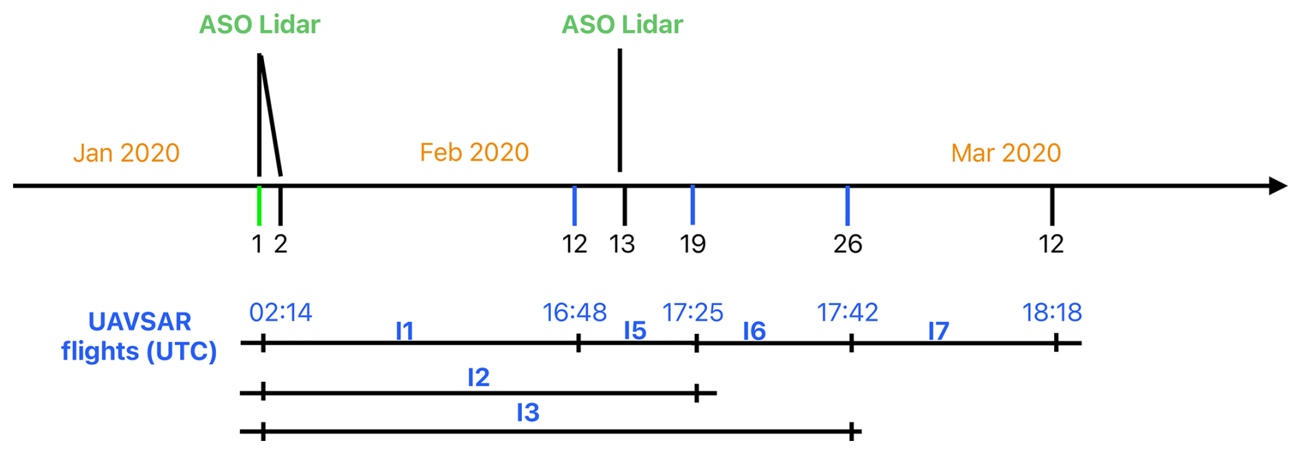
Figure 2 Timeline of the availability of UAVSAR interferometric products and ASO lidar retrievals of snow depth and SWE for the SnowEx'20 campaign over Grand Mesa. I1, I2 and I3 and I5, I6 and I7 indicate the six InSAR pairs used for data assimilation and model evaluation, respectively. The dates with green and blue tick marks represent days when the retrievals were used for assimilation in the data assimilation experiments.

Figure 2 synthesizes the availability of ASO lidar retrievals and L-band InSAR retrievals for assimilation and evaluation of model runs. Here, we use part of the data for assimilation, and the remainder is used for evaluation. As stated earlier, the L-band InSAR retrievals only provide information about relative changes in snow depth or SWE, which need to be referenced and calibrated to obtain the absolute values needed for assimilation. In the context of distributed modeling at a given resolution, this would require a spatial map of snow depth or SWE for referencing. In this study, we use the ASO lidar snow depth data at a 50 m resolution (1 February) as a reference. We aggregate the InSAR retrievals to a coarser resolution (50 m) to match with the resolution of the reference ASO lidar snow depth retrieval. Then we combine the reference snow depth with aggregated InSAR retrievals of snow depth change, I1 (1–12 February), I2 (1–19 February) and I3 (1–26 February), to obtain the absolute snow depth pattern over the GM domain on 12, 19 and 26 February, respectively. Two data assimilation experiments are conducted by assimilating total snow depth: (1) ASO lidar retrieval on 1 February (DA) and (2) ASO lidar retrieval on 1 February and referenced InSAR retrievals on 12, 19 and 26 February (DAU). We reference the InSAR retrievals by aggregating the data to a 50 m resolution grid of the ASO lidar retrievals from 1 February, which matches the date of the first InSAR pair in both cases. InSAR retrievals of snow depth change on I5 (12–19 February), I6 (19–26 February) and I7 (26 February–12 March) are reserved for independent evaluation. In both DA experiments, we assign an observational error of 10 % for the snow depth retrievals at a 50 m resolution, which is consistent with the errors from the InSAR retrievals using the UAVSAR data in this study.

3 Results

3.1 Meteorological settings

The meteorological conditions based on the HRRR forcing data, including air temperature, precipitation and wind speed, were analyzed for the GM domain (2 × 5 HRRR grids at a 3 km resolution). These environmental forcings along with temporal baselines are also the source of variability in interferometric coherence and errors in the retrievals. Figure 3 shows the time series of air temperature, wind speed and precipitation intensity for the month of February, including the first 2 weeks in March for the northwest corner of the GM domain. The month of February was generally cold and windy, with temperatures dropping below −20 °C and wind speeds reaching up to 15 m s⁻¹. The time series show cooling and warming periods at a weekly timescale, with some days where the air temperature reached above zero. However, the amplitude of cooling decreases gradually from the end of February to mid-March, with more frequent warm periods. There were a few snowfall events between 1–12 February, 19–26 February and 26 February–12 March, which varied in intensity along the GM domain.

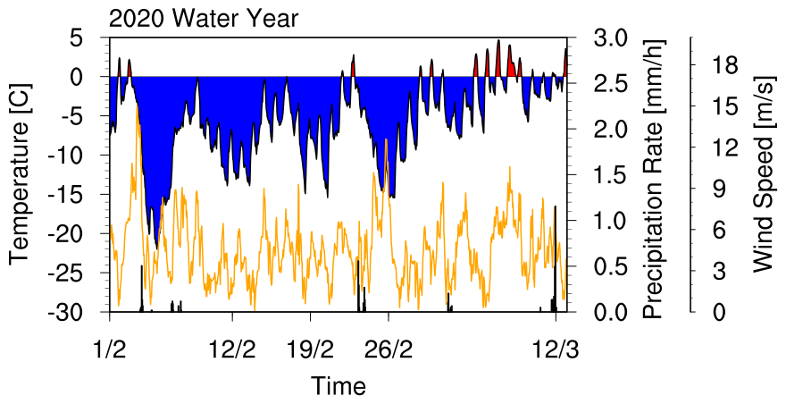
Figure 3 Meteorological data from the atmospheric model for the northwest GM subdomain showing the air temperature (blue/red), wind speed (orange) and precipitation rate (bar plot). The time axis highlights the dates when the L-band UAVSAR flight data were available for the SnowEx'20 campaign.

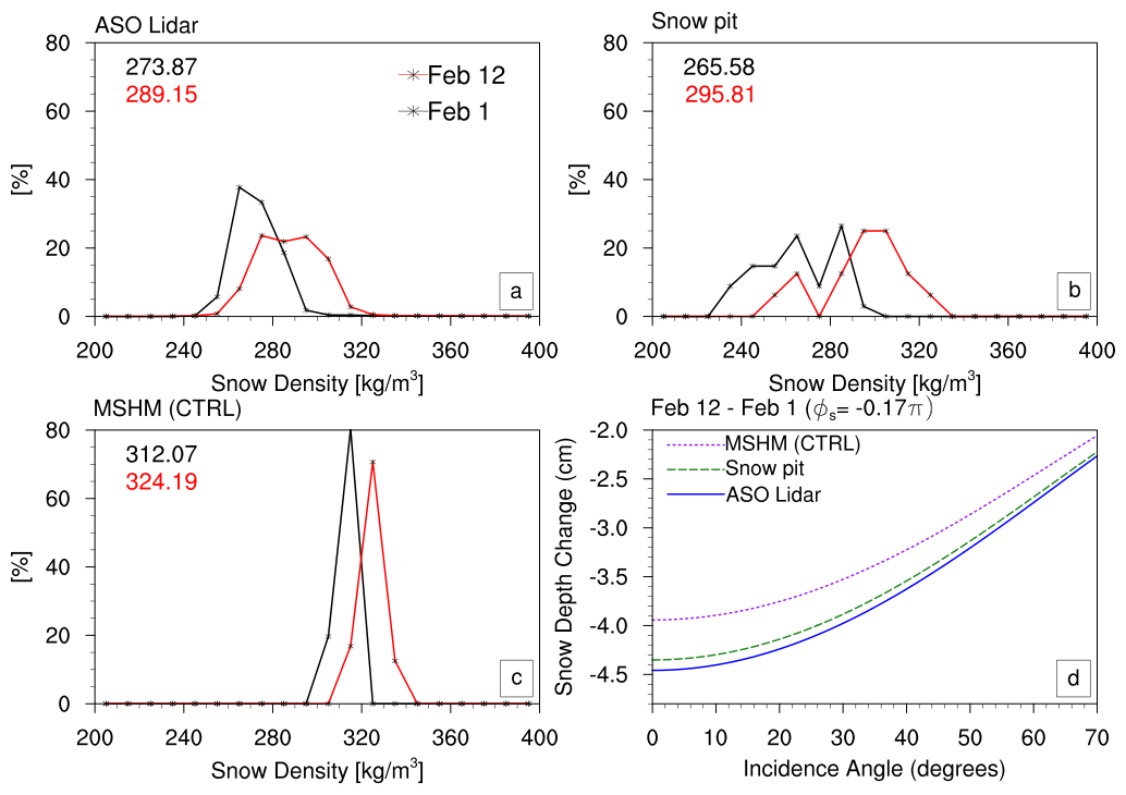
Figure 4 (a-c) Snow density distribution on 1 and 12 February from the ASO lidar data, snow pit measurements (intensive-observation period, solid-gray markers in Fig. 1) and the MSHM control run. (d) Impact of snow density on the L-band InSAR retrieval of snow depth change between the two dates as a function of the incidence angle for a fixed change in phase due to snowpack (∅_s=0.17π). The dates for ASO lidar are actually 1/2 and 13 February. We use 1 and 12 February due to the availability of InSAR phase data for these dates.

3.2 Snow density

A spatial pattern of bulk snow density is required to compute the snowpack permittivity needed for the InSAR retrieval technique. Uncertainty in snow density estimates can lead to errors in snow depth retrieval. Figure 4 shows the snow density distribution for the InSAR pair (1–12 February) using the 50 m resolution ASO lidar data, snow pit data and model estimates using a reference run (CTRL) for the GM domain. Only the snow pit data within the GM domain collected within ± 1 d of the InSAR flights were used for the analysis. All three data sets show compaction of snow between the two dates, but the model simulates slightly higher snow density for both flight dates and underestimates the spatial variance observed in the snow pit data and ASO lidar data, as was expected given the coarse resolution of the HRRR precipitation forcing (i.e., 3 km). Note that the snow density in the ASO lidar data is also from a model estimate, but it was bias corrected (i.e., locally calibrated) using the snow pit data from the SnowEX'20 campaign. In the 11 d temporal baseline, the average snow density changes by 5.6 %, 11 % and 4 % among the lidar, snow pit and model data, respectively. Here, we have to note that the snow density change in pit data could also be attributed to spatial variability besides compaction, which could be contributing to higher differences.

To examine the error in snow depth retrieval associated with the error in density, we used Eq. (1) to retrieve snow depth change for a fixed phase change due to snow. Figure 4d shows the variability in InSAR retrievals of snow depth change as a function of the incidence angle for a phase change of −0.17 π using the average snow density from ASO lidar, snow pits and the MSHM CTRL run. The error generally decreases with an increasing incidence angle. The synthetic simulation shows that a 10 % error in snow density can lead to an approximately 10 % error in snow depth estimates at lower incidence angles, with everything else being the same.

3.3 L-band retrieval of snow depth

The temporal baselines for the L-band retrieval range from 7 to 40 d, and the interferometric coherence generally decreased with increasing temporal baselines, as expected. For treeless and forested areas, the mean coherence for the 7 d temporal baseline (12–19 February) was 0.7 ± 0.15 and 0.65 ± 0.18, respectively. Similarly, for the 19–26 February pair, it was 0.6 ± 0.18 and 0.5 ± 0.2, respectively. The coherence decreased to 0.39 ± 0.16 and 0.36 ± 0.17 for the 40 d temporal baseline. These values are for the HH polarization, as it was available for all dates (see Table 2). The lower coherence for the 19–26 February pair compared to the 12–19 February pair could be attributed to environmental factors, e.g., higher wind speeds, precipitation events and intermittent warming (see Fig. 3). The forested area exhibits lower coherence than the treeless area does, suggesting the possibility of higher uncertainty in the retrievals. The above statistics are based on the NLCD land cover data at a 30 m resolution, whereas the native resolution of the InSAR retrievals from UAVSAR is on the order of a 5 m resolution, and the retrievals over forest contain information from snow depth in tree clearings as well.

Table 2 Coherence for treeless and forested environments for different retrievals.

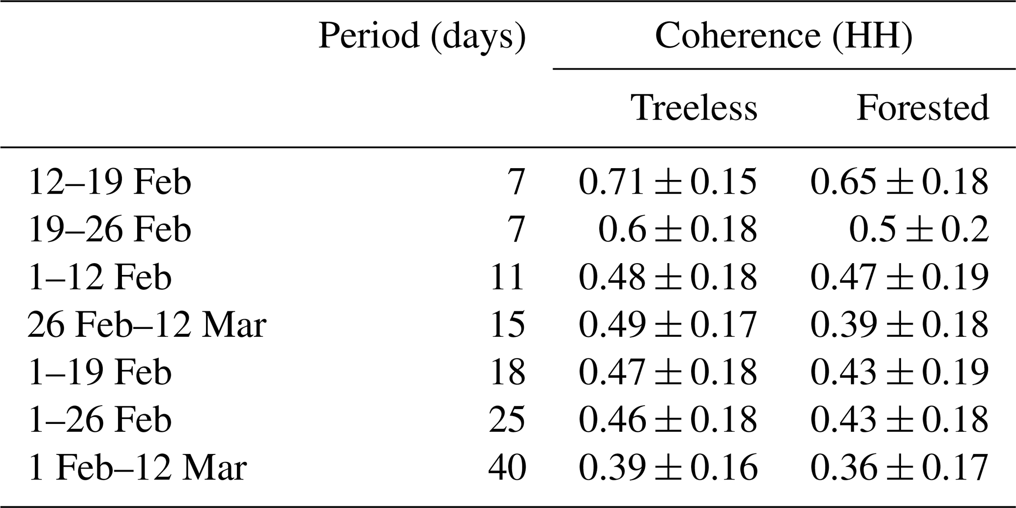
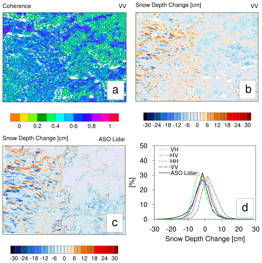
Figure 5 (a) The spatial pattern of coherence from the L-band VV polarization InSAR retrieval for the northwest GM subdomain. (b) The estimated spatial pattern of snow depth changes from the same retrieval. (c) Spatial pattern of snow depth change from ASO lidar data (1/2–13 February). (d) Distribution of change in snow depth from ASO lidar and InSAR retrievals for VV, HH, HV and VH polarizations. The InSAR retrievals were obtained from the UAVSAR flight pairs on 1 and 12 February.

3.3.1 Evaluation with ASO lidar data

The InSAR pair of 1–12 February with a temporal baseline of 11 d provides the closest concurrent pair to the ASO lidar retrieval based on 1/2 and 13 February for the comparison of the snow depth difference at the scale of a 3–5 m resolution. Figure 5a and b show the spatial pattern of interferometric coherence and snow depth change at VV polarization. Figure 5c shows the change in snow depth based on ASO lidar data for the same region. The western part of this GM subdomain is mostly dominated by snow cover over grasslands, while the eastern part contains snow cover in forested areas with relatively lower coherence. Both the lidar and L-band retrievals capture the wavy, roll-like pattern due to scouring and drifting of snow over the grasslands, which was shown earlier by Marshall et al. (2021) for a smaller area. Over the eastern part of the subdomain, which is dominated by forest, there are significant discrepancies: in regions with no snow depth change in the ASO lidar data, a decrease in snow depth is observed in the L-band retrieval.

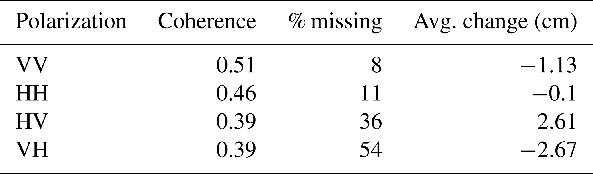
The average coherence values for this subdomain were 0.51, 0.46, 0.39 and 0.39 for VV, HH, HV and VH polarization, respectively. In addition, the missing retrievals in the radar scene were 8 %, 11 %, 36 % and 54 % of the area, respectively, for the different polarizations (see Table 3). The distribution of snow depth change for co-polarization better matches the ASO lidar data compared to the cross-polarization (Fig. 5d). The average changes in snow depth for the scene were −2.42, −1.13 and −0.1 cm, respectively, for the ASO lidar and InSAR VV and HH polarizations. The HV and VH polarizations show rightward- and leftward-shifted peaks, respectively. The impact of atmospheric correction was minimal for this retrieval. With and without atmospheric correction, the average snow depth changes for the InSAR retrieval (VV) were −1.28 and −1.13 cm, respectively, for the scene. The ASO lidar and InSAR retrieval have similar resolutions but differ in geolocations, so a quantitative spatial comparison that would require spatial interpolation was not used; instead we only explore the patterns and frequency distributions within the same extent. For the frequency distribution (Fig. 5d) between ASO and InSAR (VV), we find R = 0.97 and a root-mean-square error (RMSE) of 2.03 cm, and the previous study (Marshall et al., 2021) found R = 0.76 and RMSE = 4.7 cm using the near-surface field measured density observations in the retrieval.

Table 3 InSAR retrievals of snow depth changes at different polarizations for 1–12 February.

While the results were similar for other subdomains (not presented here), the L-band retrievals were found to show a general decrease in snow depth in the westernmost part of the GM domain dominated by forest cover, while the lidar data show a contrasting increase in snow depth. Thus, the retrievals show higher uncertainty over the forested areas, and further evaluation is needed.

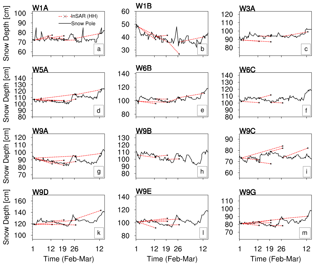
Figure 6 Comparison of the L-band InSAR retrieval (HH polarization) of snow depth with snow pole measurements for locations with different types of land cover within the GM domain (a–c: treeless; d–f: sparse trees; g–m: dense trees). For the InSAR retrieval, snow depth measurements from snow pole sites were used a reference for the repeat pass UAVSAR flight pairs.

3.3.2 Evaluation with snow pole and snow pit time series data

The snow pole data provide a time series of snow depth measurements for locations that are treeless or have sparse/dense trees and can be used for comparison with all available InSAR pairs over the GM domain. We use the snow pole data linearly interpolated in time to reference the InSAR retrievals in HH polarization and to obtain absolute snow depth for comparison. Figure 6 shows the evaluation of referenced InSAR retrievals with snow pole data for treeless land cover (Fig. 6a–c), sparse trees (Fig. 6d–f) and dense trees (Fig. 6g–m). In most cases, the L-band InSAR retrievals capture the trend in snow depth change very well for different land cover types. The RMSEs were similar for different types of land cover, with approximate values of 4–6 cm (which is consistent with earlier findings by Marshall et al. (2021) for same InSAR retrieval but using different data for evaluation). We also explored the errors in terms of InSAR pairs. The RMSEs of InSAR estimates were 5.0, 4.9, 4.4, 6.2, 7.3 and 4.2 cm for the 1–12 February (11 d), 1–19 February (18 d), 1–26 February (25 d), 12–19 February (7 d), 19–26 February (7 d) and 26 February–12 March (18 d) retrievals, respectively, at the 12 stations. The errors in InSAR retrievals are within 4 %–8 % of the absolute snow depth.

The time series from snow pits in the northwestern part of the GM domain also provide valuable snow depth measurements to evaluate the InSAR estimates. The time series contains data across treeless and forested areas (Fig. 7). Here again we use the snow pit measurements to reference the InSAR retrievals and to obtain the absolute snow depth. It must be noted that snow pit measurements were carried out at different locations within a few meters. Here, we must note that the temporal variability in the snow depth is also partly contributed by the spatial variability due to changes in the location of the pits. The snow depth was slightly higher in the treeless area compared to in the forested area, which were within 0.25 km of each other. The InSAR retrievals can capture some of the trends very well, while showing contrasting results for others, such as for the case of the snow poles. The coherence was within 0.12–0.67 and 0.33–0.79 for the treeless and forested areas, respectively. The errors were 2 %–9 % and 3 %–31 %, respectively, for treeless and forested areas. Based on the two comparisons of InSAR retrievals against snow pole and snow pit data, the errors are within 10 % for most of the retrievals, with few exceptions.

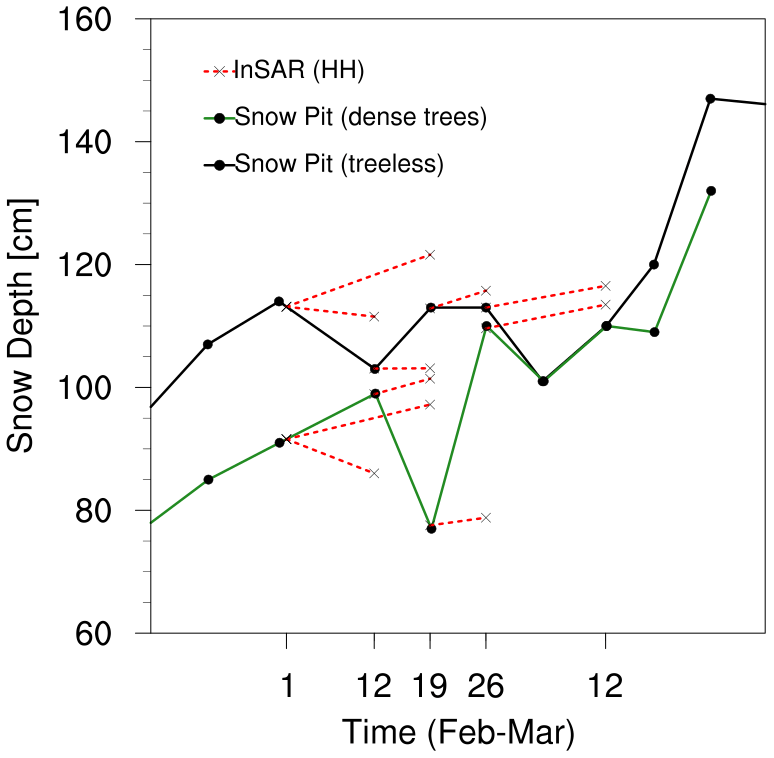
Figure 7 Comparison of the L-band InSAR retrieval (HH polarization) of snow depth with snow pit time series measurements for two locations with different types of land cover (treeless and dense trees) within the GM domain. For the InSAR retrieval, snow depth measurements from snow pit site were used a reference for the repeat pass UAVSAR flight pairs.

3.4 Data assimilation and evaluation

In this section, we explore the impact of assimilated L-band InSAR retrievals on modeled SWE and particularly on modeled snow depth. As already discussed in Sect. 2.4, we use two assimilation experiments including an open loop (without assimilation) and a reference run to explore the time evolution of modeled snowpack over Grand Mesa for the accumulation season in the water year 2020. Figure 8 shows the time series of spatially averaged modeled snow depth from the different runs. The spatial averaging was done for the grids without trees and open water over the GM domain. The filled areas represent the total ensemble spread. The assimilation of the ASO lidar snow depth on 1 February shifts the ensembles upwards and reduces the spread for both the DA and DAU runs. It shows that the reference run (CTRL) was largely underestimating snow depth. While some of the ensemble members with positive perturbations of precipitation were able to capture the actual snow depth, the ensembles with negative perturbation of precipitation underestimated the total snow depth (see the spread in the open-loop (OL) run). The assimilation of referenced InSAR retrievals for 12, 19 and 26 February (DAU runs) exhibits a small increase in snow depth for the ensemble averages compared to the DA runs.

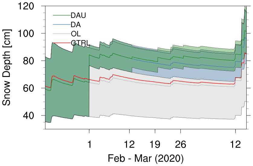
Figure 8 Time series of modeled snow depth for the CTRL, OL, DA and DAU runs. The dates when observations were assimilated are also shown by tick marks: DA (1 February) and DAU (1, 12 and 26 February) are also shown by the tick marks. The ensemble spreads for the OL, DA and DAU runs are shown by filled areas between the lines.

The modeled snowpack was also compared with in situ measurements to assess the impact of data assimilation. The modeled snow depth and SWE at a 90 m resolution were compared to snow pit data (intensive observation period, IOP, and time series snow pit data, TSD) in locations without trees. The land-cover-filtered IOP data contained snow depth and SWE from 28 January 2020 to 12 February 2020. Similarly, the land-cover-filtered TSD contained snow depth from 19 December 2019 to 17 April 2020. There were 68 IOP and 12 TSD snow pit data points available for comparison across the GM domain based on the model simulation spatial extent. The RMSE decreased from 35.2 to 18.3 cm for snow depth, and for SWE, it decreased from 8.9 to 5.9 cm. The differences in RMSE between the DA and DAU runs for these pits were negligible. The modeled snow depth was also compared against snow pole measurements for locations without trees (three locations: W1A, W1B and W3A) for the entire model simulation period. The RMSEs were 17.6, 21.2 and 27.2 cm for the CTRL run and decreased to 8.1, 21 and 20.8 cm for the DA runs. For the DAU runs, the RMSEs were 8.5, 22.2 and 19.2 cm (see Table 4).

Table 4 Root-mean-square error for modeled snow depth (cm) over treeless environments with reference to pit (IOP and TSD) and snow pole measurements.

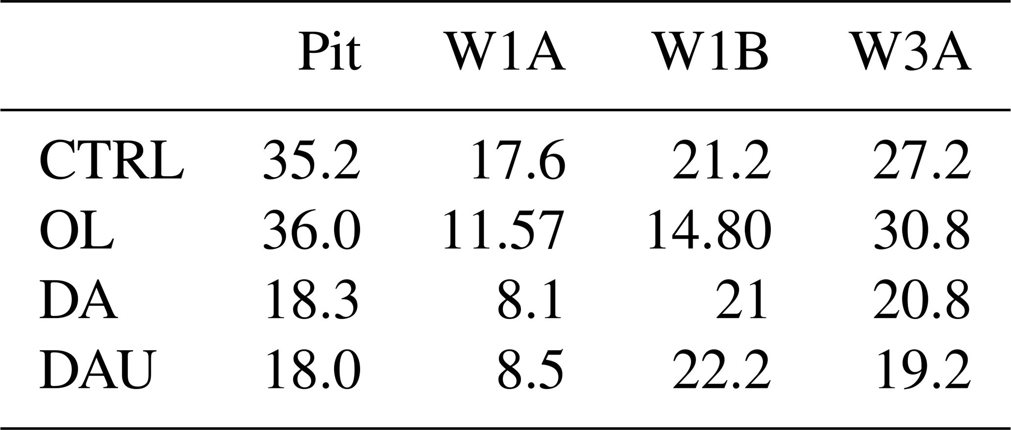
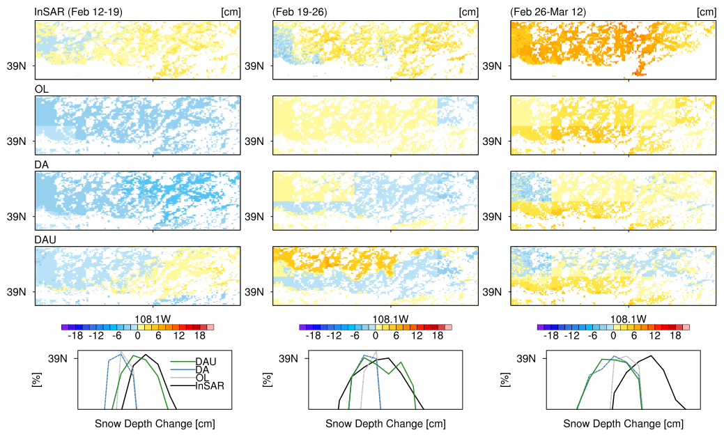
Figure 9 Spatial patterns and histograms of changes in snow depth over the GM domain for 12–19 February, 19–26 February and 26 February–12 March: (a–c) InSAR retrievals; (d–f) the ensemble-averaged open-loop run (OL); (g–i) the ensemble-averaged data assimilation run with ASO lidar data (DA); (j–l) ensemble-averaged data assimilation runs with ASO lidar and referenced InSAR data (DAU); and (m–p) the frequency distribution of snow depth change for the InSAR, OL, DA and DAU runs for the respective pairs.

The spatial pattern of the modeled snow depth can be evaluated using the reserved InSAR retrievals from the 12–19 February, 19–26 February and 26 February–12 March pairs that were not used for assimilation. Figure 9 shows the spatial pattern of snow depth change for these repeat pass retrieval dates, along with their distributions for the entire GM domain. The estimates are shown for the retrievals and for all the model runs. The InSAR data were aggregated to a 90 m resolution for comparison, and the grids with open water bodies and tree cover (sparse or dense) were all masked out. Additionally, for the ensemble runs, the spatial maps were obtained by averaging the ensembles, and the distributions are for the averaged ensembles.

The InSAR retrievals for 12–19 February and 19–26 February exhibit both increases and decreases in snow depth for the GM domain, while the retrievals for 26 February–12 March show increases in snow depth only (Fig. 9a–c). As expected, the ensemble average for the open-loop (OL) run shows spatial variability on the scale of the atmospheric forcing. The OL run shows a similar tendency to the InSAR retrievals, except for the 12–19 February pair, where it shows a decrease in snow depth (Fig. 9d–f). While the DA runs improve the total snow depth and SWE, no improvement in the snow depth change is achieved for the 12–19 February pair (Fig. 9g). In addition, there are more grids with a decrease in snow depth for the remaining two pairs (Fig. 9h and i) compared to in the OL run. Note that the DA does increase the modeled spatial variability in snow depth change.

Compared to other model runs, DAU produces the best results, with a positive increase in snow depth change (Fig. 9j and k) that is also seen in the widening of the distribution in the positive direction (Fig. 9m and n). This is due to the assimilation of InSAR data on 19 and 26 February. Since there was no assimilation of InSAR data on 12 March, there is no improvement in the modeled snow depth change for 26 February–12 March, even in DAU runs (Fig. 9i and 9l). The increase or relatively larger increase in snow depth change for DAU runs (Fig. 9j–l) is mostly for the grids where the InSAR data were available for assimilation (19 and 26 February). However, the impact of this assimilation appears local in time, and it does not produce any significant improvement for the 26 February–12 March pair compared to the DA runs. Despite the data constraints, these results indicate that the assimilation of InSAR estimates has the potential to improve the spatial pattern of modeled snow depth change. Because the snow depth evolution is cumulative, these changes will impact the overall seasonal evolution of the snowpack.

4 Discussion

The hyper-resolution InSAR retrievals resolve the wavy, roll-like patterns due to scouring and drifting of snow over the grasslands captured by the ASO lidar data in the northwestern part of GM domain, which was also shown earlier by Marshall et al. (2021). However, over forested regions, there are disagreements between the lidar and the InSAR estimates, with possible uncertainty in both data sets. The average coherence was similar for VV and HH polarization, with slightly higher values for VV polarization and lower for HV and VH polarizations. This resulted in a higher percentage of missing retrievals in cross-polarizations. The scene-wide average coherence in HH polarization for the 7 d temporal baseline (treeless area) in the GM domain is around 0.6–0.7, which is consistent with the values reported by Ruiz et al. (2022). Similarly, the coherence was around 0.5–0.65 for the forested area, indicating that the L-band can maintain good coherence over canopy, and when there is sufficient penetration depending on tree density and canopy architecture, it can be useful in measuring ground snow depth changes. The forested areas generally exhibited lower coherence, as expected, and the coherence differences between treeless and forested areas were around 14 %–23 % to 8 % for the 7 and 40 d temporal baselines, respectively. Overall, the InSAR retrievals generally compare well with in situ measurements from snow poles and snow pits over sparse and dense forests. The RMSE of the lidar measurements over the snow pole site used in the study was also around 7–8 cm for the two dates, exhibiting good accuracy. Thus, more data are required for spatial comparison in forested environments to better understand the differences between lidar and InSAR retrievals.

The interferometric coherence across the GM domain generally decreased with the increasing temporal baseline (e.g., by 44 % from the 7 to the 40 d temporal baseline). This indicates that the retrieval uncertainty and retrieval error will increase with more time between the repeat passes, as was expected. Since the underlying density of snowpack will also change between the repeat passes, the retrieval error will also increase when using a constant density in Eq. (1). In this study, the depth-weighted density averages or the average bulk density between two repeat pass dates from the reference MSHM model runs was used for the InSAR retrievals. The reference runs generally underestimated the total snow depth and SWE compared to the ASO lidar data and snow pit measurements, but the bulk snow density was slightly higher than the snow pit observations during the IOP over Grand Mesa. This indicates that the HRRR forcing used for the study underestimates the snowfall events, aside from the model uncertainty associated with wind redistribution of snow, which is not accounted for. The modeled higher bulk density could again indicate uncertainty in the fresh-snow density (Cao and Barros, 2020; Shrestha and Barros, 2025a) and compaction parameterization (e.g., Abolafia-Rosenzweig et al., 2024). The modeled layered snowpack generally shows a two-layer density profile, with an upper layer exhibiting a gradient and a near-constant density profile in the lower layer. Upon examining the density profiles, the difference in snow density profile in the lower layer varied between 1.5 %–1.8 % (19–26 February) and 6 %–7 % (1–26 February) for the 7 and 25 d temporal baselines. This could still be a lower estimate than the actual change in snow density, as shown earlier for the 11 d temporal baseline, which was 4 % and 11 % for model and snow pit observations, respectively. Therefore, the variability in snow density profiles is small for the 7 d baseline, and it is large for the 25 d baseline during the accumulation period. Aside from this, the modeled density has its own bias compared to actual snowpack density due to forcing and model structural uncertainty. However, the calibration of the retrievals to obtain the absolute snow depth change from the relative snow depth change could also compensate for these errors. Further in-depth studies are needed to better understand the sources of error.

Data assimilation of the ASO lidar snow depth reduces the error and uncertainty in the modeled snow depth. This also reduced the bulk snow density for the ensemble members with lower snow depth (compared to the CTRL run) by 4 %–5 %, as new snow with a lower density is added on the top by the repartition algorithm (Shrestha and Barros, 2025a). These ensemble members (DA; Fig. 9h and i) also exhibited lower or negative snow depth change for 19–26 February and 26 February–12 March compared to OL ensembles, which is reflected in the ensemble averages over the GM domain. However, the assimilation of referenced InSAR retrievals (DAU) produces an increase in snow depth changes in the ensemble average compared to in the DA runs. The impact is most apparent in the grids of the GM domain where the data were available for assimilation. This produced the best distribution of snow depth change compared to observations, showing the potential of InSAR retrievals for improving the modeled snowpack. It also demonstrates HRRR underestimation of snowfall between the dates of the InSAR pairs (e.g., between 26 February and 12 March), and it explains the small snow depth differences in the OL runs compared to those in the InSAR retrievals. The OL shows the increase in snow depth due to snowfall just before 12 March (see Fig. 3), albeit underestimated, as indicated by the difference in magnitude between the InSAR retrievals and the OL snow depth changes. Likewise, the impact of assimilating InSAR retrievals, which improves the simulated snow depth changes (as seen for the first two pairs), highlights the need for a high temporal resolution of SAR measurements.

5 Conclusion

This study shows that InSAR retrievals are useful to improve the snowpack simulation and capture its spatial and temporal variability. The assimilation of hyper-resolution retrievals of snow depth is equivalent to a downscaling of the precipitation forcing with a bias correction, besides the additional contribution from physical processes not resolved by the model at the given scale. The RMSE of the InSAR retrievals of absolute snow depth change at a native resolution compared to snow pole measurements over different types of land cover were within 4–6 cm, which corresponds to less than 10 % of the absolute snow depth. However, reference snow depth or SWE is essential to obtain absolute snow depth or SWE for assimilation purposes, which poses a challenge in an operational context. In this situation, one would start from snow-free conditions and build up the absolute snow depth from InSAR retrievals using the prior estimates as a reference. Accurate calibration of the estimated relative snow depth change or SWE will be important to minimize retrieval errors. Further work is also essential for InSAR retrievals in forested areas and complex terrain. Future studies are needed to advance a general framework for calibrating InSAR retrievals and obtaining absolute snow depth or SWE for assimilation into the models.

Appendix A

The atmospheric delay experienced by a microwave signal can be estimated by integrating the atmospheric refractivity along the line of sight from the surface to the airborne sensor height. Neglecting the impact of the ionosphere on the UAVSAR flying at a height of z_s, the scaled-up atmospheric refractivity of moist air ($N=(n-\mathrm{1}){\mathrm{10}}^{\mathrm{6}}$), where n is the refractive index, is given by

$$N(x,z)=k_{\mathrm{1}}{\displaystyle \frac{P}{T}}+(k_{\mathrm{2}}-k_{\mathrm{1}}){\displaystyle \frac{e}{T}}+k_{\mathrm{3}}{\displaystyle \frac{e}{T^{\mathrm{2}}}}+k_{\mathrm{4}}{W}_{\text{cl}},$$

where P is pressure [hPa], T is air temperature [K], e is vapor pressure [hPa], W_cl is liquid water content [kg m⁻³], n_e is ionization and f is frequency. The remaining terms are constants: k₁ =  0.776 K Pa⁻¹, k₂ = 0.716 K Pa⁻¹, k₃ = 3750 K² Pa⁻¹ and k₄ = 1430 m³ kg⁻¹. Based on the work of Smith and Weintraub (1953), the above relation is restricted to certain limits of the variables for an accuracy of 0.5 % in N(x,z). The limits in this case restrict its use to temperatures of −50 to +40 °C, total pressures of 200 to 1100 mb, water vapor partial pressures of 0 to 30 mb and a frequency range of 0 to 30 GHz.

N(x,z) can be further decomposed into the mean and turbulent parts of a radar scene as

$$N(x,z)=\stackrel{\mathrm{‾}}{N}\left(z\right)+N^{\prime }\left(xz\right),$$

where $\stackrel{\mathrm{‾}}{N}\left(z\right)$ is the average vertical stratification for the given resolution of the atmospheric model (here 3 km), and N^′(xz) is the deviation from the average profile along the location x in the radar scene (within the atmospheric grid). Neglecting the turbulent terms, zenith delay L for the mean part can be computed as

$$L=\underset{z_{\text{ref}}}{\overset{z_{\mathrm{s}}}{\int }}\left(k_{\mathrm{1}}{\displaystyle \frac{P}{T}}+(k_{\mathrm{2}}-k_{\mathrm{1}}){\displaystyle \frac{e}{T}}+k_{\mathrm{3}}{\displaystyle \frac{e}{T^{\mathrm{2}}}}\right)\mathrm{d}z.$$

Using $\mathrm{d}P=-\mathit{\rho }g\mathrm{d}z$ and $\mathit{\rho }=P/R_{\mathrm{d}}T$, where ρ is air density [kg m⁻³], R_d = 287.053 $\mathrm{J}{\mathrm{kg}}^{-\mathrm{1}}{\mathrm{K}}^{-\mathrm{1}}$ is the dry-gas constant and g is acceleration due to gravity, we obtain

$$\begin{array}{rl}L=& -{\mathrm{10}}^{-\mathrm{6}}\left(k_{\mathrm{1}}{\displaystyle \frac{R_{\mathrm{d}}}{g}}\left(P\right(z_{\mathrm{s}})-P(z_{\text{ref}}\left)\right)\right)\\ & +{\mathrm{10}}^{-\mathrm{6}}\underset{z_{\text{ref}}}{\overset{z_{\mathrm{s}}}{\int }}\left((k_{\mathrm{2}}-k_{\mathrm{1}}){\displaystyle \frac{e}{T}}+k_{\mathrm{3}}{\displaystyle \frac{e}{T^{\mathrm{2}}}}\right)\mathrm{d}z\end{array}.$$

The first term of the right side is the hydrostatic correction term, and the second term is the wet-correction term. The atmospheric phase delay along the line of sight (LOS) can then be estimated using the microwave wavelength (λ) and incidence angle (θ_inc) as

$${\mathrm{\varnothing }}_{\text{atm}}={\displaystyle \frac{\mathrm{4}\mathit{\pi }}{\mathit{\lambda }}}{\displaystyle \frac{L}{\text{cos}\left({\mathit{\theta }}_{\text{inc}}\right)}}.$$

The above simple approximation for computing atmospheric phase delay along the LOS could introduce additional uncertainty (Wang et al., 2021). More importantly, since SAR interferograms are not sensitive to image-wide phase biases, there will be no horizontal delay differences over flat terrain. However, for a radar scene with terrain, the differences in the vertical refractivity during both acquisitions will affect the phase difference between two arbitrary-resolution cells with different topographic heights (Hanssen, 2001). Therefore, the contribution of tropospheric stratification to the interferogram will only be present if the radar scene has resolution cells with different elevations. Thus, we compute the differential atmospheric phase delay between locations with maximum elevation (z_ref=p) and all other locations (z_ref=q) in the radar scene for two SAR acquisition times, t₁ and t₂, as

$$\mathrm{\Delta }{\mathrm{\varnothing }}_{\text{atm}}={\displaystyle \frac{\mathrm{4}\mathit{\pi }}{\mathit{\lambda }\text{cos}{\mathit{\theta }}_{\text{inc}}}}\left[\left(L_{\mathrm{p}}^{t_{\mathrm{1}}}-L_{\mathrm{q}}^{t_{\mathrm{1}}}\right)-\left(L_{\mathrm{p}}^{t_{\mathrm{2}}}-L_{\mathrm{q}}^{t_{\mathrm{2}}}\right)\right].$$

Then the phase change contribution due to snowpack is estimated as

$$\mathrm{\Delta }{\mathrm{\varnothing }}_{\mathrm{s}}=\mathrm{\Delta }{\mathrm{\varnothing }}_{\text{InSAR}}-\mathrm{\Delta }{\mathrm{\varnothing }}_{\text{atm}}.$$