Historically consistent mass loss projections of the Greenland ice sheet

Mass loss from the Greenland ice sheet is a major contributor to global sea-level rise and is expected to intensify with ongoing Arctic warming. Given the threat of sea-level rise to coastal communities, accurately projecting future contributions from the Greenland ice sheet is crucial. This study evaluates the expected sea-level contribution from the ice sheet until 2100 by conducting an ensemble of standalone ice sheet simulations using the Community Ice Sheet Model (CISM). We initialize the ice sheet to closely match observed geometry by calibrating basal friction parameters and using regionally downscaled surface mass balance (SMB) forcing from various Earth system models (ESMs) and the ERA5 reanalysis. Using a historically consistent approach, we reduce model drift while closely reproducing observed mass loss over the historical period. We evaluate the effects of using absolute SMB values vs. prescribing SMB anomalies for future projections, identifying minimal differences in projected sea-level contributions. Our projections suggest sea-level contributions of 32 to 69 mm under SSP1-2.6 (Shared Socioeconomic Pathway), 44 to 119 mm under SSP2-4.5, and 74 to 228 mm under SSP5-8.5 by 2100. In our setup, variations in the initial state of the ice sheet only have a minimal impact on projected sea-level contributions, while climate forcing is a dominant source of uncertainty.

1 Introduction

Increased mass loss from the Greenland ice sheet is expected to be a major contributor to future global sea-level rise. Accurately projecting Greenland's response to future climate is challenging for various reasons, including uncertainties arising from poorly constrained boundary conditions, model formulations, and the inability to adequately resolve or represent all relevant physical processes. With the goal of improving projections of sea-level contribution from ice sheets, several studies have investigated various aspects that contribute to these uncertainties. Goelzer et al. (2013), for example, evaluated the effects of physical model formulations, such as the handling of surface mass balance (SMB) forcing, outlet glacier dynamics, and basal lubrication, as well as the model resolution of projected contributions of the Greenland ice sheet to global sea-level rise. Spatial representation in terms of the grid spacing and resolution of bedrock topography and the interaction with outlet glacier forcing were also the focus of a study by Rückamp et al. (2020), while the effect of elevation feedback parameterization on modeling results was investigated by Edwards et al. (2014a). Sea-level projections have been found to be highly sensitive to climate forcing and ice sheet model uncertainty, which includes uncertainties stemming from structural differences between ice sheet models, as well as uncertainties related to specific modeling choices, such as the experiment setup (Bindschadler et al., 2013; Goelzer et al., 2020b). The Ice Sheet Model Intercomparison Project for CMIP6 (ISMIP6), for example, assessed uncertainties related to climate forcing and quantified ice sheet model uncertainty by comparing projections with different ice sheet models using various climate forcings from the CMIP5 archive (Goelzer et al., 2020b). In accordance with previous studies, ISMIP6 identified the initial representation of the modeled ice sheet as a major source of uncertainty for ice sheet projections. Many simulations showed a large model drift, resulting from the initialization to the present day and insufficient representation of historical mass loss.

The initialization of ice sheet models to represent present-day conditions is a critical aspect of projecting future ice sheet behavior. Past studies have compared various initialization methods and investigated their impacts on projections (Aschwanden et al., 2013; Yan et al., 2013; Adalgeirsdóttir et al., 2014; Goelzer et al., 2018). The initialization of ice sheet models can be done using various approaches, each with distinct advantages and limitations. One possible method involves simulating full glacial cycles that have preceded the present-day climate while allowing for the ice sheet geometry to freely evolve, ensuring internal consistency in the surface mass balance (SMB), ice thickness, velocity field, and ice temperature (e.g., Huybrechts and Wolde, 1999; Yang et al., 2022). This approach produces an ice sheet that is in balance with its past forcing and provides the ice sheet state with a long-term memory of past conditions. However, so-called paleo-spin-ups often result in substantial deviations from observed ice sheet geometries, potentially introducing biases in future projections. As an alternative, data assimilation techniques prioritize matching present-day observations, yielding ice sheet configurations in close agreement with observed conditions (Seroussi et al., 2011; Larour et al., 2012; Gillet-Chaulet et al., 2012; Pollard and Deconto, 2012; Brinkerhoff and Johnson, 2013; Lee et al., 2015). Matching the observed state of the ice sheet is possible using inverse methods or calibration, where poorly constrained parameters are adjusted to achieve a close match with observed surface velocities (e.g., Morlighem et al., 2010; Seroussi et al., 2013; Gillet-Chaulet et al., 2016) or ice sheet surface elevation (e.g., Pollard and Deconto, 2012). However, this method may induce unwanted model drift due to mismatching boundary conditions, model physics, or assimilation targets and a lack of past climate memory. Inverting for less constrained variables such as bed friction may thus lead to compensation effects (Berends et al., 2023). Furthermore, issues arise regarding the choice of SMB representation during initialization, as different choices of reference SMB may lead to divergent projections of future mass loss. Several studies (Pattyn et al., 2013; Seroussi et al., 2014; Goelzer et al., 2018) have emphasized the need to further improve on initialization methods for ice sheet modeling and advocated for further exploration of combined approaches, which, for example, allow for a relaxation after data assimilation.

Projections of future ice sheet mass loss are often performed using climate forcing in terms of SMB anomalies with respect to a reference SMB (Edwards et al., 2014a; Goelzer et al., 2020b; Payne et al., 2021). Forcing with absolute SMB output from climate models is generally difficult due to the bias that many climate models exhibit (Knutti and Sedláček, 2013; Vial et al., 2013; Eyring et al., 2016). The anomaly approach ensures the removal of biases and allows for the combination of SMB forcing from different sources. This is often necessary when simulating a time span that includes the historical period as well as a future projection or when performing an ensemble of projections that start from the same initial state but use future forcing from various climate models.

In this study we address the question of initialization by examining how different initial SMB products impact the projected ice sheet mass loss using an inverse method that minimizes ice thickness differences relative to the observed reference ice thickness. We present historically consistent projections of future sea-level contribution and evaluate the impact of forcing projections with absolute SMB values vs. prescribing SMB anomalies. We thereby complement existing estimates of sea-level contribution from the Greenland ice sheet on a decadal to centennial timescale while sampling uncertainties related to climate forcing and modeling choices.

In the following section (Sect. 2) we describe the ice sheet model and the experimental setup before presenting the results in Sect.3. We examine the initial state in Sect. 3.1, the historical period in Sect. 3.2, and the projections in Sect. 3.3. We conclude with a discussion of the results in Sect. 4.

2 Model description and experimental setup

2.1 The Community Ice Sheet Model

We project contributions to global mean sea level from the Greenland ice sheet until the year 2100 by performing an ensemble of standalone simulations with the Community Ice Sheet Model (CISM) (Lipscomb et al., 2019), which is a 3D thermomechanically coupled higher-order model. Given the 2D bed elevation and ice thickness fields, the 3D temperature field, and relevant boundary conditions, the model calculates the ice velocity by solving a depth-integrated viscosity approximation of the Stokes equations (Goldberg, 2011) on a structured rectangular grid. The 3D temperature enters into the viscosity equation via a temperature-dependent rate factor before an effective viscosity is calculated by integration over all vertical layers (see Eqs. 2, 5, and 24 in Lipscomb et al., 2019). Simulations in this study are run using 11 irregularly spaced vertical layers which become more tightly spaced towards the base and a horizontal grid resolution of 4, 8, and 16 km. We apply a power law for basal sliding based on Weertman (1957):

$$\begin{array}{}\text{(1)}& {\displaystyle }{\displaystyle }{\mathit{\tau }}_{\mathrm{b}}=k^{-\mathrm{1}/p}{N}^{q/p}{\mathit{u}}_{\mathrm{b}}^{\mathrm{1}/p},\end{array}$$

where τ_b is basal shear stress, k is a friction coefficient which is based on the thermal and mechanical properties of ice and related to bed roughness, N is the effective pressure, and u_b is the basal velocity. The exponents are set to p=3 and q=1, following Cuffey and Paterson (2010). The thermal evolution of the ice sheet is determined by a prognostic temperature solution. Basal meltwater is removed immediately. Climate forcing at the upper ice boundary is applied via providing SMB and surface temperature (ST) fields. All floating ice is assumed to calve immediately. We justify the neglect of floating ice based on the rare occurrence of floating ice in Greenland. While floating ice does exist in Greenland in the form of ice tongues located at the termini of outlet glaciers, these ice tongues are limited in number and extent (Reeh, 2017). Mass loss processes of the Greenland ice sheet are therefore primarily determined by surface processes and outlet glacier dynamics, while sub-shelf melting can be neglected (Broeke et al., 2009).

2.2 Climate forcing

Climate forcing for the simulations comes from 10 different Earth system models (ESMs), 9 CMIP6 models and 1 CMIP5 model, as well as from the ERA5 reanalysis (Hersbach et al., 2020). We use climate forcing from the low-emission SSP1-2.6 scenario, the intermediate-emission SSP2-4.5 scenario, and the high-emission SSP5-8.5 scenario to sample a wide range of possible Shared Socioeconomic Pathways. A complete list of all ESM–scenario combinations used in this study can be found in the Appendix (Table A1). All ESM simulations have been dynamically downscaled over Greenland with the Modèle Atmosphérique Régional (MAR) v3.12 (Fettweis et al., 2017). Since MAR produces SMB and ST forcing on a fixed ice sheet geometry, the SMB–elevation feedback is not accounted for in the forcing dataset. The SMB–elevation feedback is a positive feedback mechanism between the changing ice sheet surface and the atmosphere (Edwards et al., 2014a, b). As the ice sheet loses mass, its surface elevation decreases. In lower elevations the ice sheet surface is exposed to higher temperatures due to the adiabatic lapse rate of air. This enhances surface melt and therefore alters the SMB. We account for the SMB–elevation feedback by parameterizing it based on local vertical gradients of runoff, according to a correction method used by Franco et al. (2012). The locally applied SMB in each grid cell is therefore corrected depending on elevation change and local changes in runoff in the surrounding cells so that

$$\begin{array}{}\text{(2)}& {\displaystyle }{\displaystyle }\text{SMB\_applied}=\text{SMB}\left(h\text{\_fixed}\right)+\mathrm{d}h{\displaystyle \frac{\mathrm{d}\text{RU}}{\mathrm{d}z}},\end{array}$$

where SMB(h_fixed) is the MAR SMB, produced on the fixed ice sheet geometry; dh is the elevation change relative to the reference elevation (of the initial ice sheet state); and $\frac{\mathrm{d}\text{RU}}{\mathrm{d}z}$ is the runoff gradient calculated from several surrounding cells. We use gradients in runoff rather than gradients in SMB because SMB is affected by precipitation, which does not have a consistent gradient with elevation. The temperature boundary condition (ST) for the thermal evolution of the ice sheet is corrected in a similar manner. For a detailed description of the method, see Sect. 6.1 and Fig. S11 in Franco et al. (2012). Atmospheric forcing is represented by prescribing either the absolute SMB and ST or anomalies with respect to a reference period.

We follow Slater et al. (2019, 2020) and use the ISMIP6 parameterization (Goelzer et al., 2020b) to represent interaction of the ice sheet with the ocean. Retreat of marine-terminating outlet glaciers is prescribed as a maximum ice front position (via a retreat mask) applying a semi-empirical parameterization, which linearly relates retreat of terminus position ΔL to changes in submarine melt at the glacier front:

$$\begin{array}{}\text{(3)}& {\displaystyle }{\displaystyle }\mathrm{\Delta }L=\mathit{\kappa }\mathrm{\Delta }\left(Q^{\mathrm{0.4}}\text{TF}\right),\end{array}$$

where Q denotes subglacial discharge, parameterized as mean summer surface runoff from the ice sheet as provided by MAR; TF denotes thermal forcing, which is taken into account by depth-averaged (200–500 m) far-field ocean temperature from the ESMs aggregated over seven drainage basins around Greenland; and κ is a calibrated sensitivity parameter, which accounts for the uncertainty in the sensitivity of outlet glacier response to climate forcing (see Sect. 3.2 in Slater et al., 2019). We sample this uncertainty using three different values for κ covering the median, 25th percentile, and 75th percentile of values from a distribution of calibrated values using observations of retreat for nearly 200 tidewater glaciers over the period of 1960–2018 (Slater et al., 2019). These different sensitivities are referred to as medium, high, and low sensitivity. The parameterization calculates retreat as a weighted average over several drainage basins, rather than for single glaciers, which allows for the application of the parameterization without explicitly resolving individual outlet glaciers.

2.3 Experimental setup

The setup of the simulations is similar to the ISMIP6 protocol (Goelzer et al., 2020b), except for a dedicated historical experiment. Simulations consist of three parts: the spin-up, which results in an initial ice sheet assigned to 1960; a historical run from 1960 to 2014; and a projection from 2015 to 2100.

2.3.1 Spin-up

The goal of the spin-up is to produce an ice sheet that is in balance with its forcing and closely resembles recently observed conditions. During a period of 5000 years we apply an annual mean SMB and ST of a reference period, which we choose to be 1960–1989, a period during which the ice sheet is assumed to have been in relative balance with its forcing (Broeke et al., 2009). At the start of the spin-up the ice sheet is set to recently observed bedrock topography and ice surface elevation as mapped by BedMachine v3 (Morlighem et al., 2017). For reasons of numerical stability and in order to ensure a stable interpolation from high resolution to a coarser CISM grid, the topography data are first smoothed with a Gaussian filter before being interpolated onto the model grid using a nearest-neighbor approach. The ice temperature is initialized with an advective–diffusive balance between the surface temperature at the upper boundary and the geothermal heat flux according to data from Shapiro and Ritzwoller (2004) at the lower boundary. During spin-up, the basal friction parameters are calibrated to nudge the ice surface elevation towards observed conditions following Pollard and Deconto (2012), which implies that the basal temperature only has a limited effect on the sliding. The obtained basal friction parameters are then held constant for the rest of the simulation, which we assume to be justified for a centennial timescale. It should be noted that this approach leads to the compensation of other modeling uncertainties, such as, for example, uncertainty in basal heat flux, as well as inaccuracies in forcing through the bed roughness (Berends et al., 2023). To minimize the already small residual model drift and to ensure the long-term stability of the initial ice sheet, we let all initialized ice sheet configurations relax for an additional 1000 years, for the 4 km grid resolution, and for 500 years for the coarser resolutions on their respective bed friction field. We assign the resulting ice sheet geometry to the beginning of 1960 in our simulations and hence forward call this state the initial state or the initialization.

We divide our ensemble of projections into two subsets, depending on the use of SMB during spin-up:

1. For the first ensemble we produce one single initialization by applying SMB from the ERA5 reanalysis downscaled with MAR, which matches well with observations over the reference period (Vernon et al., 2013). We call the ensemble using this initialization the ERA5-init ensemble and refer to the downscaled SMB as ERA5-SMB.

2. For the second ensemble we perform multiple spin-ups using the reference SMB from each ESM downscaled with MAR. We thereby obtain multiple initial ice sheet configurations, each with a different friction field and small variations in ice surface elevation. The ensemble using this initialization approach will henceforth be called the ESM-init ensemble, and the SMB products from the different ESMs, which are again downscaled using MAR, will in summary be referred to as ESM-SMB and 〈ESMname〉-SMB for a specific ESM.

2.3.2 Historical period

We define the historical period as extending from 1960 to 2014.

All runs in the ERA5-init ensemble branch off from the one single ERA5 initialization, which also implies that the friction field is the same for all members of this ensemble. This historical run is forced with SMB and ST from the ERA5 reanalysis, downscaled with MAR (neglecting the SMB–height feedback), which reproduces observations well (Vernon et al., 2013). Following Slater et al. (2019) (Sect. 2.2.2), surface runoff data for calculating retreat in this historical run are estimated using the regional climate model RACMO (Noël et al., 2018), which was forced at its boundaries by ERA-40 and ERA-Interim. Observations of ocean temperature used for the retreat parameterization come from the Hadley Centre EN4.2.1 dataset (Good et al., 2013). We perform three different historical runs, each using a different sensitivity (κ in Eq. 3) to outlet glacier retreat forcing.

The historical runs in the ESM-init ensemble branch off of each ESM initialization and are forced with absolute values of SMB and ST from the respective ESM (dynamically downscaled with MAR). Note that ESMs generally do not reproduce the observed interannual and interdecadal climate variability over the historical period (Knutti and Sedláček, 2013; Deser et al., 2012). Outlet glacier retreat over the historical period is calculated using surface runoff from the respective ESM MAR simulation, while ocean thermal forcing comes directly from the respective ESM. For each ESM, we again carry out three different historical runs using different sensitivities to the outlet glacier retreat forcing. In total we produce 33 historical runs.

2.3.3 Future projections

Following the historical run, future projections start in 2015 and go to the year 2100. In both ensembles all three sensitivities to outlet glacier retreat forcing are taken into account.

In the ERA5-init ensemble, projections are forced by anomalies with respect to the annual mean SMB and ST of the reference period (1960–1989) from the same ESM that is used for the projection such that

$$\begin{array}{}\text{(4)}& {\displaystyle }{\displaystyle }\text{SMB}\left(t\right)=\text{SMB\_ref\_ERA5}+\text{SMB\_anomaly}\left(t\right)\end{array}$$

with

$$\begin{array}{}\text{(5)}& {\displaystyle }\begin{array}{rl}{\displaystyle }\text{SMB\_anomaly}\left(t\right)& {\displaystyle }=\text{SMB\_ESM}\left(t\right)\\ {\displaystyle }& {\displaystyle }-\text{SMB\_ESM\_ref(1960–1989\hspace{0.17em}mean)}.\end{array}\end{array}$$

Note that ESM-SMB always refers to dynamically downscaled SMB. This commonly used approach (e.g., Goelzer et al., 2020b) ensures the use of high-quality forcing during spin-up and allows for a correction of biases in the ESM forcing. Furthermore, it has the advantage of being flexible and computationally efficient, as only one initialization is needed for the entire ensemble of projections. It comes, however, at the cost of introducing a possible inconsistency in the forcing, when transitioning from the ERA5 forced historical simulation to the projection.

For the ESM-init ensemble, projections are instead forced by prescribing absolute values of SMB and ST, following the approach used for the historical period such that SMB(t)=SMB_ESM(t). Forcing with an absolute SMB from the same model ensures a consistent forcing stream of the simulation from initialization throughout the historical period and the projections. Note that values of absolute SMB and surface temperature in the ensemble ESM-init can technically be divided into a reference part (annual mean of the ESM over the period of 1960–1989) and an anomaly part such that $\text{SMB\_ESM}\left(t\right)=\text{SMB\_ref\_ESM}+\text{SMB\_anomaly}\left(t\right)$. This means that forcing, in terms of anomalies, is identical in both ensembles because, in both cases, the anomalies are calculated with respect to the ESM annual mean of the reference period.

Bedrock elevation is kept constant throughout the simulation, as we assume isostatic adjustment to be small on a centennial timescale and therefore negligible for the projections (Sutterley et al., 2014; Wake et al., 2016). Sea-level contributions are calculated relative to the year 2015 based on ice volume above flotation and include a density correction that accounts for density differences between ocean water and fresh meltwater (Goelzer et al., 2020a). For conversion of ice volume change to sea-level equivalent we assume a constant ocean area of 3.625×10¹⁴ m² (Gregory et al., 2019).

We run projections with forcing from 10 different ESMs, sampling 3 SSPs, 3 sensitivities to outlet glacier retreat forcing, and the 2 different initialization approaches. All projections using ESM-init are run at 4 km grid resolution, while all ERA5-init experiments are run at three different grid sizes (4, 8, and 16 km). In total, our simulation dataset consists of 192 projections.

3 Results

3.1 Initial state

By the end of the initialization, ice thickness, temperature, and velocity fields of all modeled ice sheet configurations are close to steady state. With a mass change ranging from −41 Gt (0.11 mm sea-level equivalent) to −110 Gt (0.3 mm sea-level equivalent) over 100 years, the residual drift is very limited for all initialized ice sheet configurations.

Simulated ice mass ranges from 2.68×10⁶ to 2.71×10⁶ Gt. In comparison, observations of the Greenland ice sheet suggest an ice mass of $\mathrm{2.73}\pm \mathrm{0.02}\times {\mathrm{10}}^{\mathrm{6}}$ Gt (assuming the same ice density of 917.0 kg m⁻³ as used for the simulations, instead of an ice density of 916.7 kg m⁻³) (Shepherd et al., 2020). Slight variations in the experiment's initial mass can be attributed to the limited ability of the inversion in the initialization approach to compensate for biases in the initial SMB. We assess the model state at the end of the initialization by comparing the modeled ice thickness to the observed ice thickness, calculating the root mean square error (RMSE) (Fig. 1). Across most ice sheet configurations, the RMSE remains below 30 m, except in the ACCESS1.3-init configuration, which reaches an RMSE of 45 m. Despite this exception, the simulations closely align with observational data. For a 2D comparison of modeled and observed ice thickness in the ERA-init configuration, see Fig. S1 in the Supplement. Comparing the initial ice thickness across all configurations to the target ice sheet geometry, 90 % of the simulated values in the ESM-init ensemble show absolute differences of less than 33 m. In the ERA5-init configuration, 90 % of the differences are below 16 m.

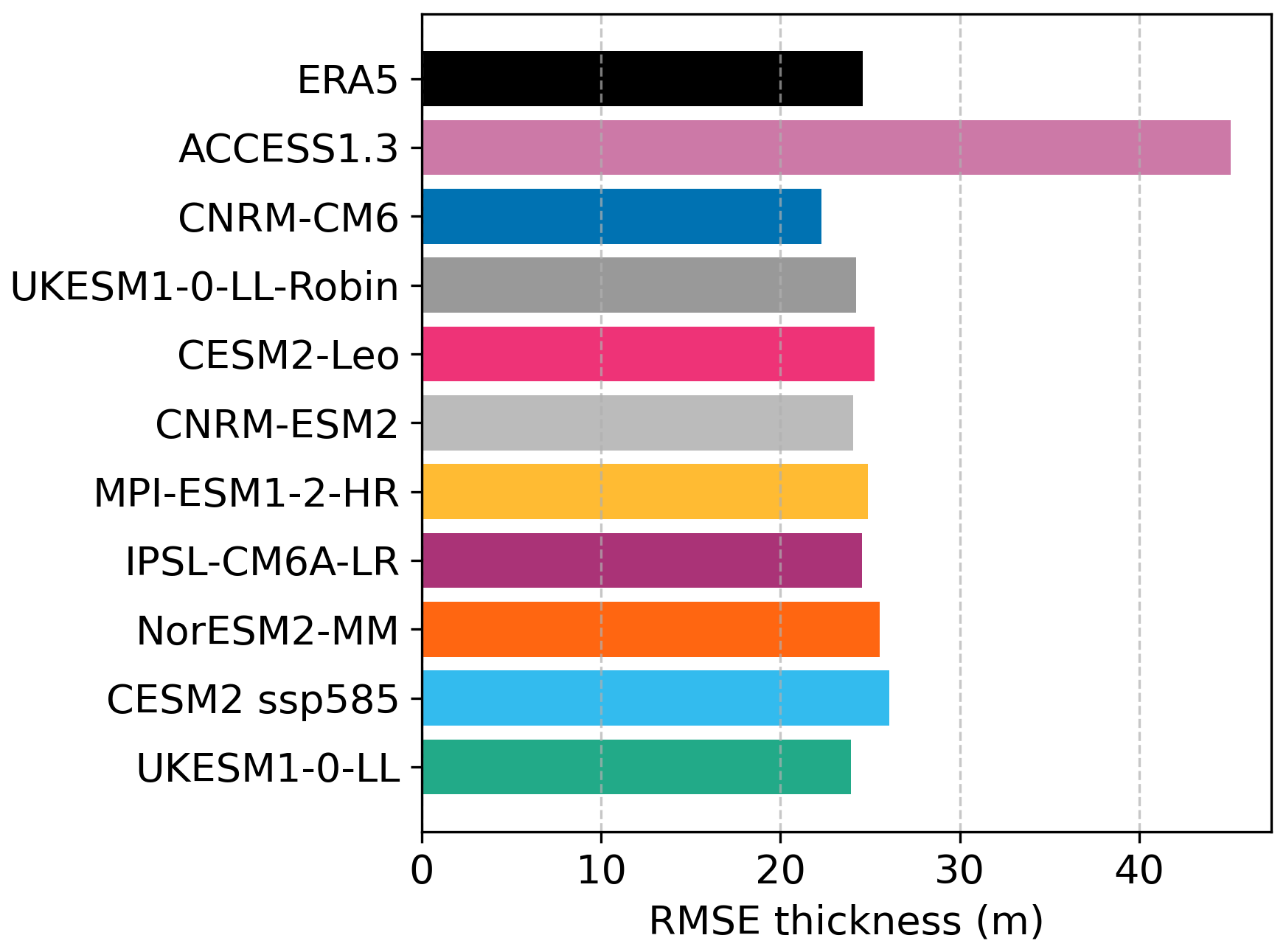
Figure 1 Root mean square error (RMSE) of simulated ice sheet thickness at the end of the initialization compared to observations (Morlighem et al., 2017). To reduce spatial correlation, RMSE was calculated for grid cells regularly subsampled in space. Shown is the median value for different offsets of the sampling.

Additionally, we compare the horizontal surface ice velocities generated by the ERA-init configuration with observations reported by Joughin et al. (2016). The simulated velocity fields show close agreement with the observed data, even though the model was calibrated to match observed ice surface elevation. A comparative visualization of these velocity fields is presented in Fig. S2.

Figure 2 shows the ice sheet state after the initialization using forcing from the ERA5 reanalysis. A comparison of all members of the ESM-init ensemble to ERA5-init can be found in Figs. S2–S4. The differences in reference SMB, ice surface elevation and bed friction field reveal no common pattern. Some models display higher SMB values around the margins, while others display lower SMB values. In the interior of the ice sheet, differences in SMB approach 0 for all ESM-init instances. Differences in SMB generally coincide with differences in surface elevation, e.g., regions of higher SMB correlate with regions of higher surface elevation. Differences in the bed friction field mirror the differences in SMB so that areas of increased SMB result in areas of lowered friction.

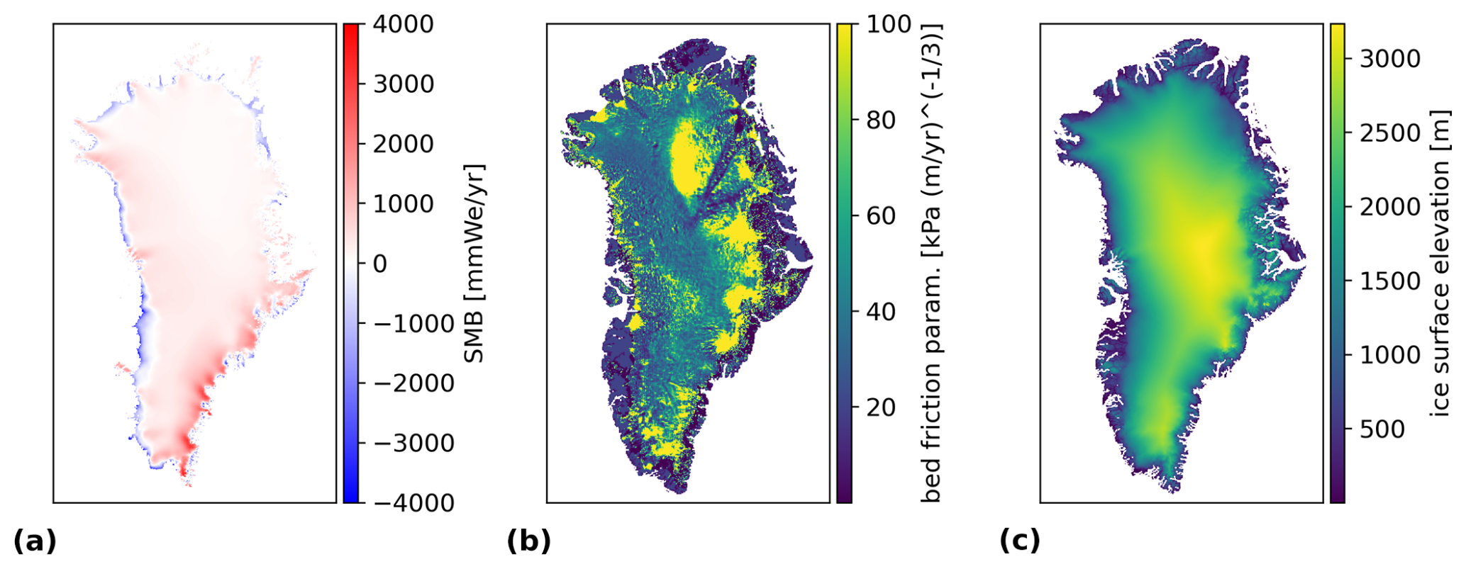
Figure 2 SMB (a), bed friction parameter (b), and ice surface elevation (c) at the end of the initialization of ERA5-init.

To illustrate the effect of different reference SMB forcing instances with a concrete example, we continue with a more in-depth analysis of the comparison of ERA5-init to the initialization produced with SMB from the Norwegian Earth System Model (NorESM2-MM) from the ESM-init ensemble, which is our in-house model (Fig. 3). Differences in SMB are most pronounced around the margins of the ice sheet, where NorESM2-MM-init generally exhibits higher SMB values than ERA5-init. This leads to differences in the resulting bed friction fields, which compensate for the difference in SMB during inversion for the same target geometry by increasing the slipperiness in areas where high SMB values produce ice that is too thick and vice versa. This way, ice is being evacuated more effectively from areas with a surplus, while it is retained in areas where modeled ice thickness is lower than targeted. The inferred bed roughness of the NorESM2-MM initialization is lower, especially in areas of higher SMB, except for parts of the northwestern and central regions of the ice sheet. While the target geometry is the same for both initializations, the ice sheet thickness at the end of the initialization procedure still differs slightly around parts of the margins. This is a residual due to the inability of the inversion process to fully compensate for discrepancies between forcing and target geometry, which, in this case, leads to thicker margins of the initial ice sheet for the NorESM2-MM initialization.

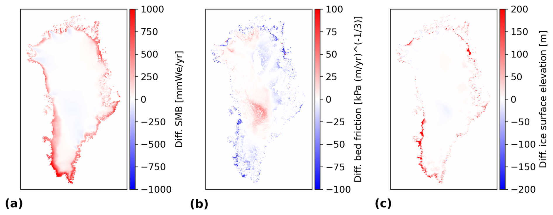
Figure 3 Differences between the initialization with NorESM2-MM and the initialization with ERA5: SMB (a), friction parameter (b), and ice surface elevation (c).

To demonstrate how a mismatch between SMB and the friction field would propagate into a biased ice sheet geometry in the absence of further calibration, we perform a supplementary experiment, where we examine the ice sheet's response to sudden changes in SMB during the initialization. We perform the ERA5 spin-up without relaxation and change the SMB forcing to that of NorESM2-MM for the relaxation period. We let the ice sheet relax in this configuration for 1000 years. In other words the ice sheet is spun up using ERA5-SMB and is then relaxed on the corresponding friction field while applying ESM-SMB, which does not match the friction field. The resulting ice sheet geometry significantly deviates from ERA5-init (Fig. 4). It is the mismatch between SMB and the friction field that leads to a deviation from ERA5-init. This mismatch results in a buildup of the ice sheet, where higher friction prevents efficient evacuation of excess ice, while it leads to a thinning of the ice sheet in areas where low friction inhibits ice sheet growth. Differences are prominent in the same regions where differences in ice surface elevation between NorESM2-MM-init and ERA5-init occur (e.g., at the southwestern margins of the ice sheet, as well as in distinct areas of the northern margin; see Fig. 3c) but are more pronounced in this simulation. This experiment illustrates how a discrepancy between SMB and the friction field can result in a biased ice sheet geometry if no further calibration is applied.

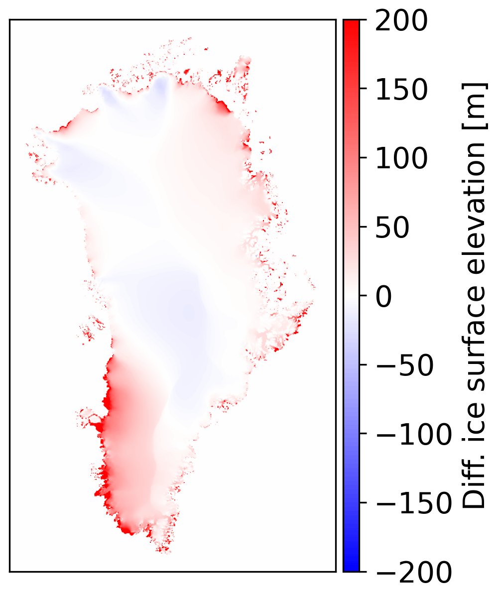
Figure 4 Difference in ice surface elevation compared to ERA5-init for an ice sheet configuration that was spun up with ERA5-SMB and relaxed using NorESM2-MM-SMB.

3.2 Historical period

The mass loss of different ice sheet configurations over the historical period is presented in terms of time-dependent mass change (Fig. 5) and in terms of sea-level contribution relative to the year 2015 (Fig. 6). The latter approach, by design, causes all simulations to converge to 0 at 2015. In all simulations, the ice sheet's contribution to sea-level rise increases over the historical period, although at varying rates. All model members capture the increased sea-level contribution of the ice sheet starting in the 1990s, but the onset and slope of this trend differ between simulations. These differences are due to the fact that the ice sheet configurations exhibit different initial ice masses and that the ESM forcings do not accurately reproduce the observed interannual and interdecadal climate variability and are possibly biased. Over the observed period from 1992 to 2014, most ESM-init simulations fall within the range of the observed sea-level contribution, assuming a maximal error correlation. However, in some cases, the ESM-init simulations either exceed or fall short of the observed values for parts of the period. For example, between 2001 and 2010, the NorESM2-MM-init simulation shows slightly lower sea-level contribution than observed, while the CESM2-Leo-init simulation exceeds the observed sea-level contribution between 1992 and 2005.

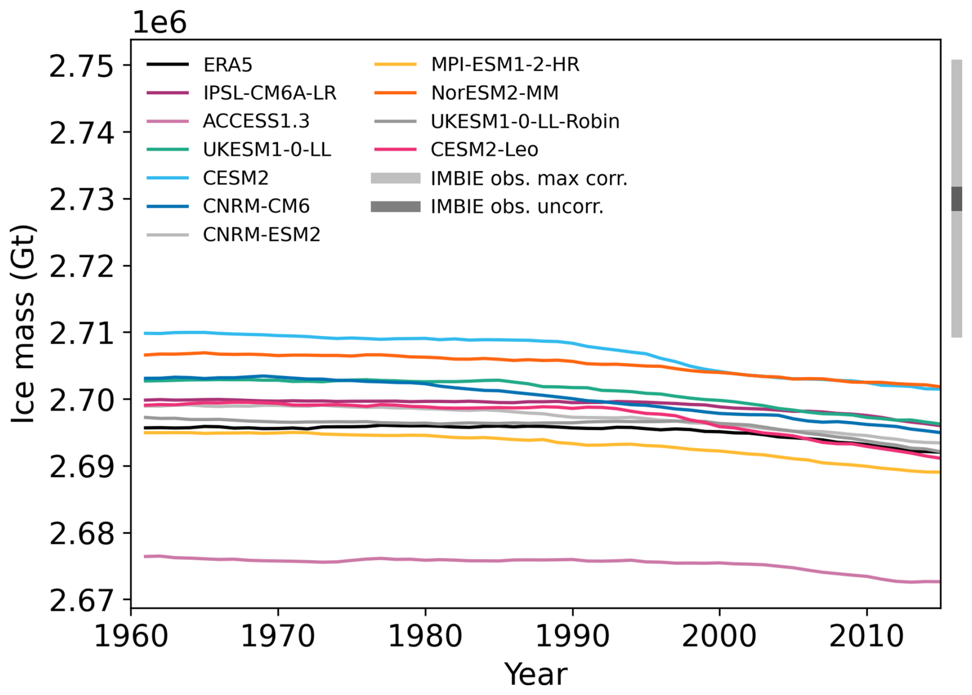
Figure 5 Ice mass over the historical period. All simulations are shown for medium sensitivity to outlet glacier retreat forcing. The grey shadings represent the range of observed mass loss data from Shepherd et al. (2020), with light-grey shading indicating the assumption of maximal error correlation and dark-grey shading indicating uncorrelated errors. The treatment of errors by the Ice Sheet Mass Balance Inter-comparison Exercise (IMBIE) involves two approaches: maximal error correlation assumes that errors across different datasets are fully correlated, leading to a wider uncertainty range (light-grey shading). In contrast, uncorrelated errors assume no correlation between errors in different datasets, resulting in a narrower uncertainty range (dark-grey shading).

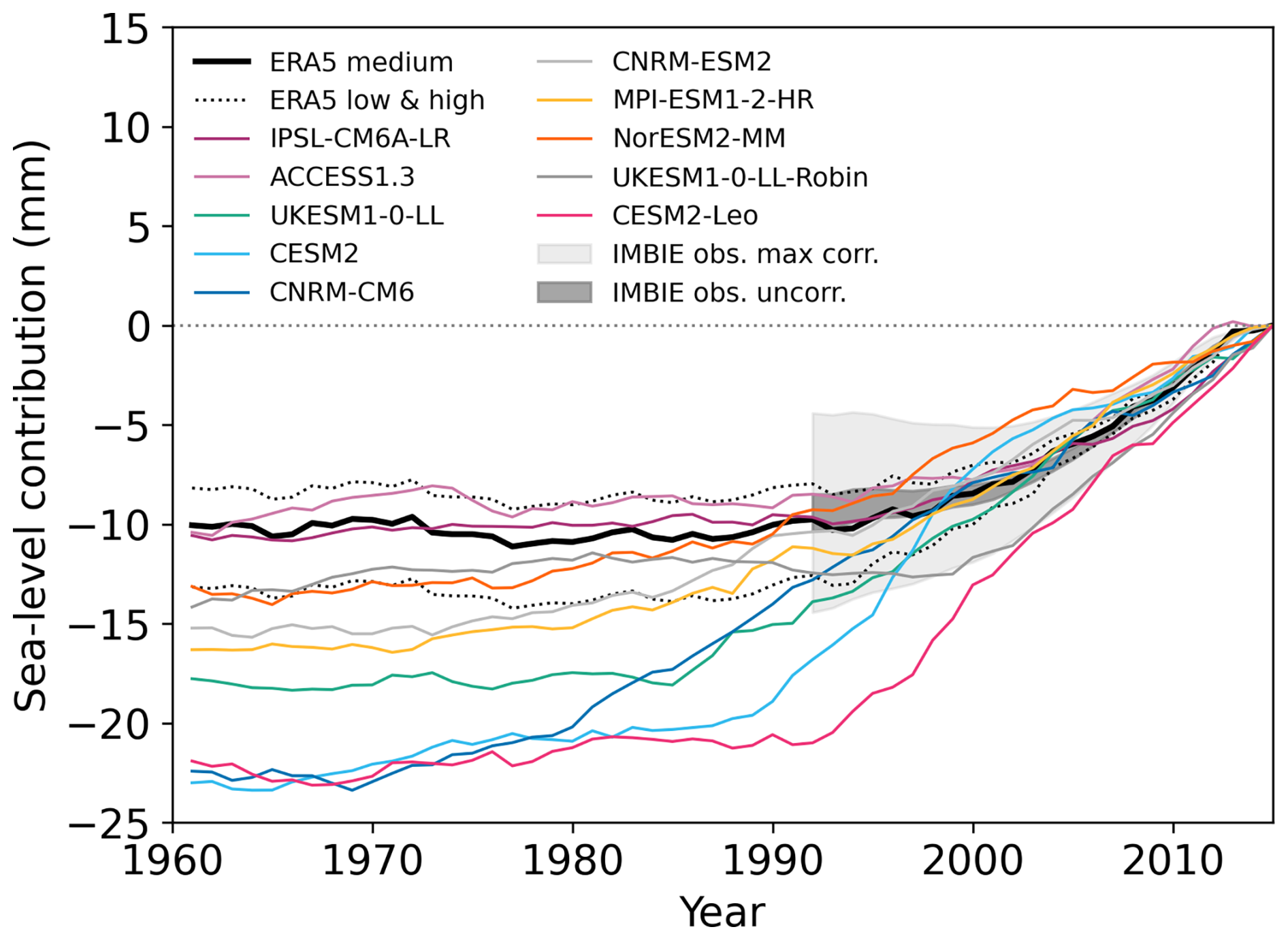
Figure 6 Historical sea-level contribution relative to 2015. The grey shadings represent the range of observed mass loss data from Shepherd et al. (2020), with light-grey shading indicating the assumption of maximal error correlation and dark-grey shading indicating uncorrelated errors. For consistency with the IMBIE observations, the sea-level contribution is calculated without applying a density correction. The ESM-init simulations (colored lines) are shown only for medium sensitivity to outlet glacier retreat forcing, while all sensitivity levels are displayed for the ERA5-forced simulations (black lines). For further explanation of the IMBIE treatment of errors, see the caption of Fig. 5.

Simulations initialized and forced with ERA5 reanalysis data show good agreement with the observed mass change, which we attribute to the accurate replication of interannual and interdecadal variability in the forcing data (Vernon et al., 2013). This is particularly true for the simulation with medium sensitivity to outlet glacier retreat forcing, which remains within the narrow range of the observed sea-level contribution assuming uncorrelated errors (see dark-grey shading in Fig. 6). The ERA5 simulations with both low and high sensitivity to retreat forcing also lie well within the range of the observed sea-level contribution, assuming maximal error correlation.

After performing historical simulations, we carry out control experiments, for which the SMB and ST anomalies are set to 0 (Fig. 7). This approach ensures that the control forcing is representative of the 1960–1989 reference period. The control experiments yield a sea-level contribution ranging from 2.3 to 7.3 mm by the year 2100. This projected contribution is primarily due to the ice sheet's response to the historical forcing, with only a small portion attributable to residual drift from the initialization process (see Sect. 3.1). During the historical simulation, the ice sheet is subjected to increasingly negative SMB forcing, including interannual variability, leading to continued mass loss beyond 2015. To account for this delayed response of the ice sheet to past forcing, it is essential to include the effect of historical forcing in future projections. Therefore, we have chosen not to subtract the control experiments from our projections, enhancing the historical consistency of our results. This approach represents a significant improvement over previous studies, such as those in ISMIP6 (Goelzer et al., 2020b), where substantial drifts persisting after the ice sheet initialization were subtracted from the projections.

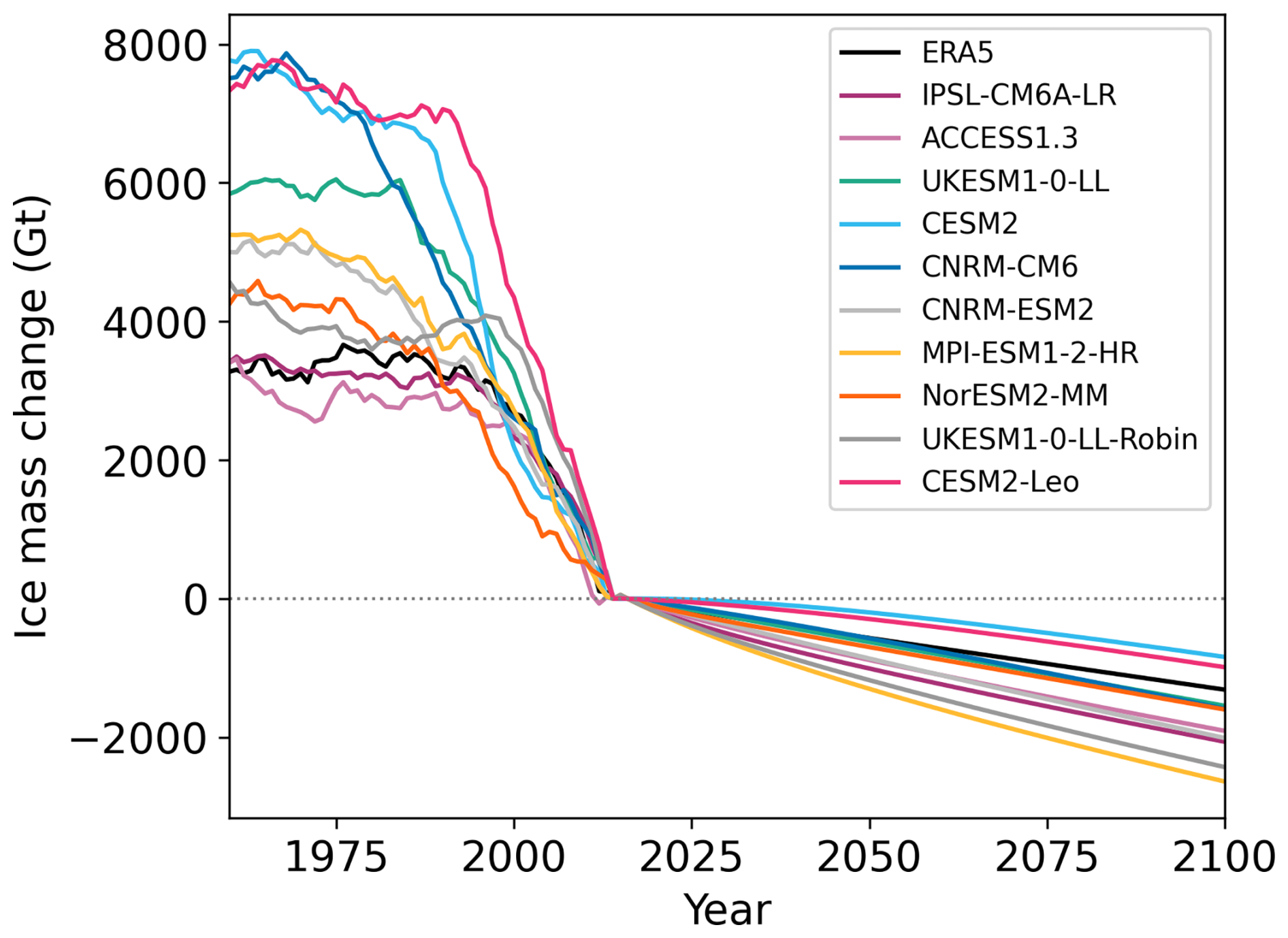
Figure 7 Mass loss (in Gt) of different ice sheet configurations over the historical period and subsequent control projections with forcing set to the mean of the reference period of 1960–1989.

3.3 Projections

Considering the good match with observations of the historical simulations with medium sensitivity to outlet glacier retreat forcing, we focus our subsequent presentation of results for future projections on this parameter choice. Sea-level contribution increases under all scenarios (Fig. 8), indicating progressive mass loss of the ice sheet. While for the low- and intermediate-emission scenarios (SSP1-2.6 and SSP2-4.5) the increase in sea-level contribution is almost linear over the entire century, mass loss accelerates significantly under the high-emission scenario (SSP5-8.5) towards the end of the century. Average rates of change under SSP1-2.6 are 0.7 mm yr⁻¹ for the period of 2040–2050 and 0.6 mm yr⁻¹ for the period of 2090–2100, which is similar to present-day observations (Rignot et al., 2008; Shepherd et al., 2012). For the SSP2-4.5 scenario, rates of change amount to 0.8 mm yr⁻¹ over the period of 2040–2050 and 1.1 mm yr⁻¹ over the period of 2090–2100, respectively. In contrast, SSP5-8.5 forced projections exhibit a rate of change of 0.9 mm yr⁻¹ over the period of 2040–2050, which increases to 3.7 mm yr⁻¹ over the period of 2090–2100. This means that under the SSP5-8.5 scenario, the sea-level contribution from the ice sheet in the second half of the century is more than 4 times faster than in the first half. This information is vital for coastal planning strategies to effectively design protection and adaptation measures.

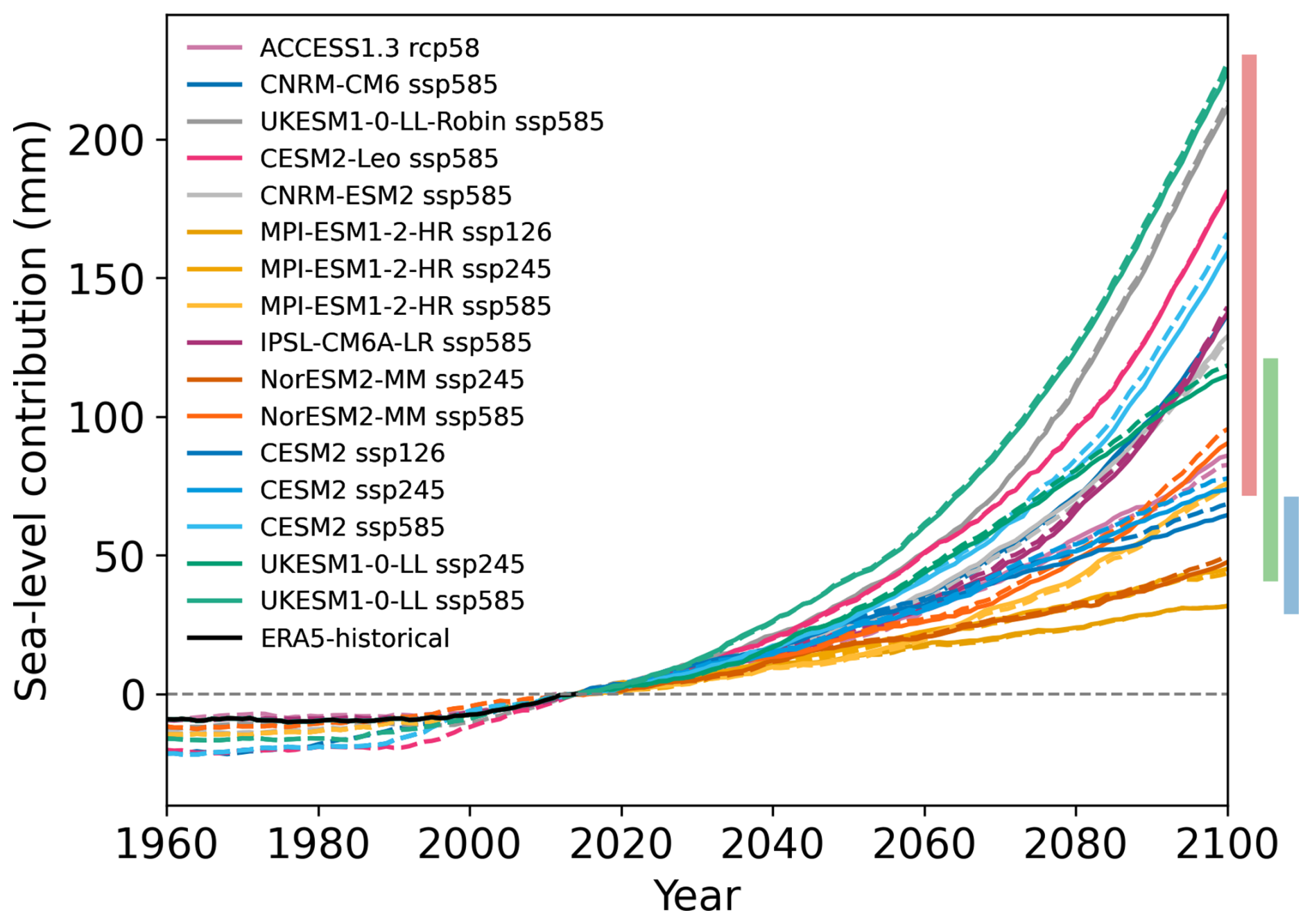
Figure 8 Projected sea-level contributions relative to 2015. Solid lines are projections starting from ERA5-init; dashed lines are the respective ESM-init projections. All simulations were run with medium sensitivity to outlet glacier retreat forcing. Vertical bars denote the range of projected sea-level contribution per scenario: SSP5-8.5 (red), SSP2-4.5 (green), and SSP1-2.6 (blue).

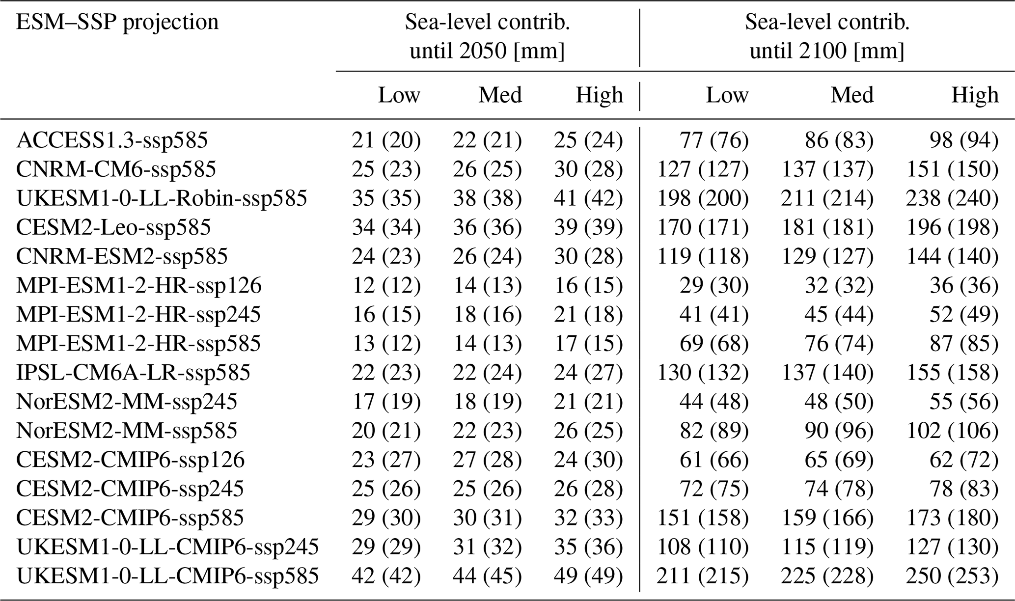
Taking the year 2015 as a reference, the total sea-level contribution by 2100 is projected to be between 32 and 69 mm for the low-emission scenario and between 44 and 119 mm (74 and 228 mm) for the intermediate-emission (high-emission) scenario, respectively. The ensemble shows a notable overlap of the intermediate-emission scenario with the low- and the high-emission scenario, demonstrating high uncertainty in the projections stemming from the climate forcing. This uncertainty is most pronounced for the SSP5-8.5 scenario, where the range of the projected sea-level contribution amounts to 154 mm. The highest contribution of the entire ensemble comes from the UKESM1-0-LL-SSP5-8.5 forced projection, while the lowest contribution in the SSP5-8.5 group (forced with MPI-ESM1-2-HR) is almost as low as the highest contribution in the SSP1-2.6 group (forced with CESM2). Detailed results for all projections are given in Table A1.

Differences in sea-level contribution originating from different initializations (ESM-init vs. ERA5-init) are rather small compared to the ensemble spread due to climate forcing. At the end of 2100, projections initialized with ESM forcing deviate from their respective ERA-initialized projections by −3.2 to +7.1 mm (Fig. 9), which is equivalent to −4.1 % to 6.6 % relative to the total contribution. There is no clear trend as to whether the ESM-init projections over- or underestimate sea-level contributions relative to their ERA5-initialized counterparts. The mean absolute difference is only 2.7 mm (equivalent to 2.9 %), implying a relatively low impact of the forcing used for initialization and the resulting friction field on the projections for the used modeling strategy.

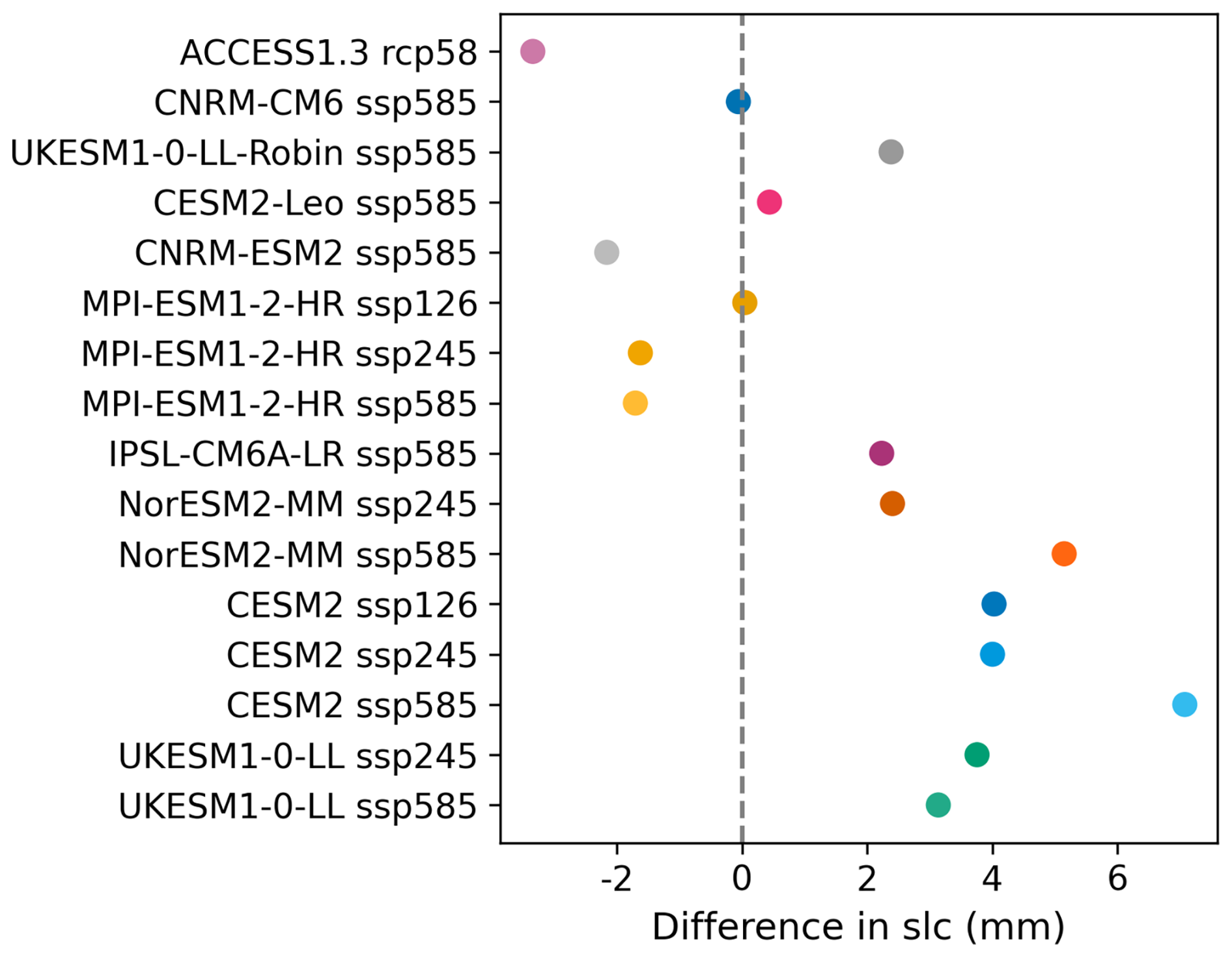
Figure 9 Differences in sea-level contribution (SLC) until 2100 for projections starting from an ESM initial state vs. starting from an ERA5 initial state.

To further assess the impact of the initial ice sheet state on the resulting sea-level contribution in the year 2100, we analyze how various state parameters of the initial ice sheet (SMB, bed friction, and ice sheet thickness) relate to differences in the sea-level contribution in the year 2100 (Fig. 10a–c). All parameters are spatially integrated around the margins of the ice sheet, where differences in ice sheet thickness to the ERA5-init ice sheet and changes during projection are most pronounced. This is done by selecting grid cells where the horizontal ice velocities at the surface of the ERA5-init ice sheet exceed 50 m yr⁻¹ (Fig. 10d). We fit the relative differences in the SMB, friction parameter, and initial ice thickness (ESM-init − ERA5-init) to the relative differences in the projected sea-level contribution of the corresponding projections (ESM-init − ERA5-init) using a linear regression. While bedrock friction (Fig. 10b) shows only a weak linear relationship to the projected sea-level contribution, the initial SMB (Fig. 10a) and ice thickness (Fig. 10c) exhibit a strong linear relationship to the projected sea-level contribution. Projections that initially start with relatively thicker ice sheet margins tend to yield higher sea-level contributions. This is a result of the higher SMB at the margins provided by the “biased” ESMs during the spin-up period. As the inversion is unable to completely counteract the buildup of thick margins, a residual remains after the initialization is complete. Therefore, those initial ice sheet configurations have more mass at their margins available for removal by the runoff and retreat of outlet glaciers when the same anomalous forcing is applied, which leads to higher mass loss. This effect is further promoted by lower friction around the margins, which is a result of the inversion process, as the model is trying to compensate for ice that is too thick.

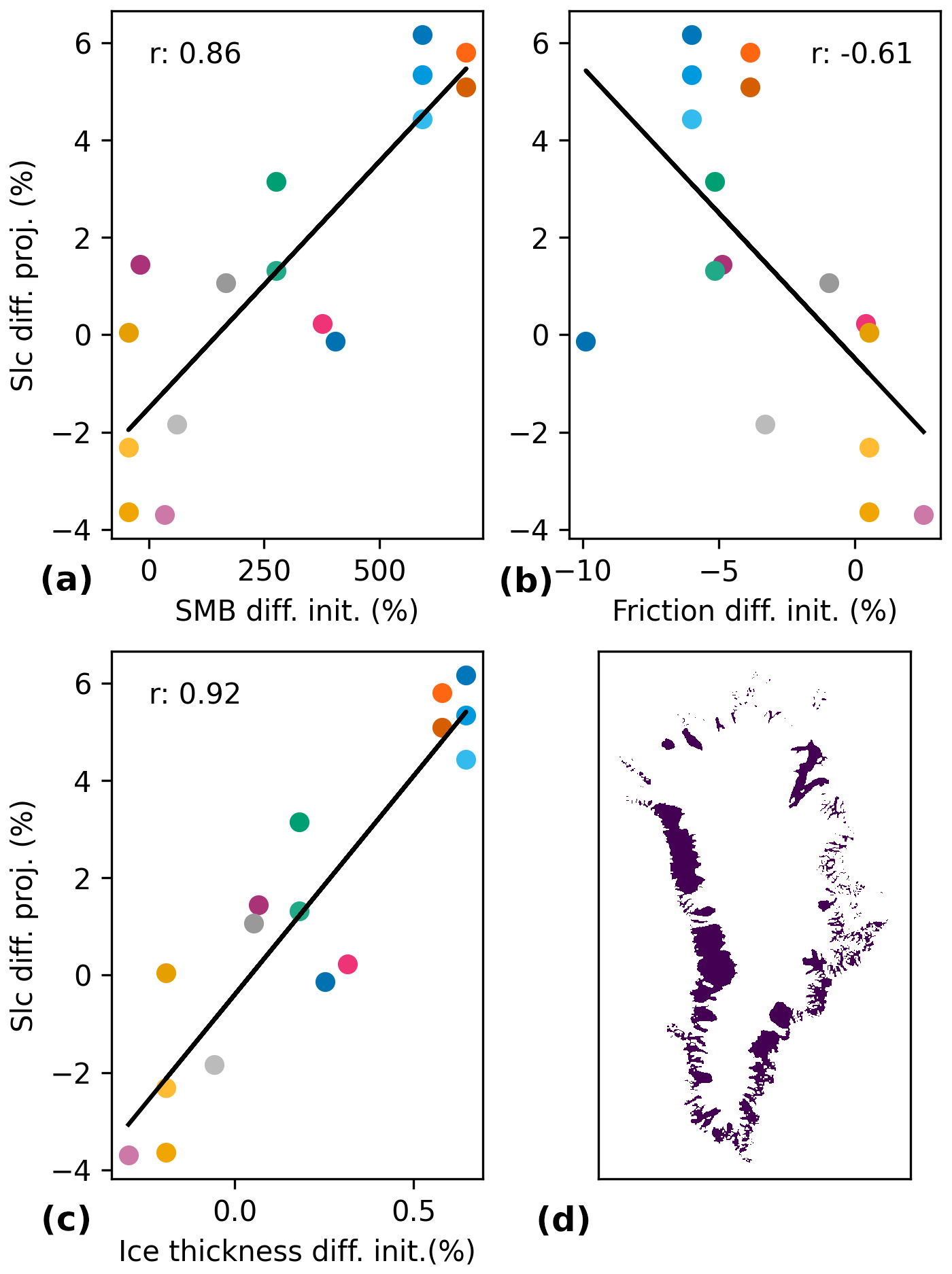
Figure 10 Relative differences in sea-level contribution by 2100 vs. relative differences in filtered and spatially integrated SMB (a), friction coefficient (b), and ice thickness (c) after ice sheet initialization. Black lines in (a–c) denote linear fits. Correlation coefficients as a measure of the goodness of the fit are given within each panel. The color scheme is the same as in Fig. 8. Panel (d) shows the masked area of ERA5-init where surface velocities are larger than 50 m yr⁻¹. The mask is used to chose areas over which the SMB, friction coefficient, and ice thickness of each ESM-init are integrated and compared against ERA5-init. Note that the analysis has been proven to be robust to variations in the filter velocity, as similar results have been found with different velocity filters (30–80 m yr⁻¹), as long as the filtered area represents the margin of the ice sheet. For a detailed description, see the main text.

To capture the uncertainty in the tidewater glacier response to climate forcing and to quantify the range of possible future sea-level contributions, we apply low-, intermediate-, and high-emission scenarios for the outlet glacier retreat parameterization to all projections, following Slater et al. (2020). We compare sea-level contributions for all three emission scenarios (Fig. 11). The mean spread in the sea-level contribution due to outlet glacier retreat forcing for the projections forced with the low-emission scenario is 5 mm. For projections forced with the intermediate-emission scenario, the mean spread amounts to 11 mm, while the mean spread increases to 25 mm for projections forced with the high-emission scenario.

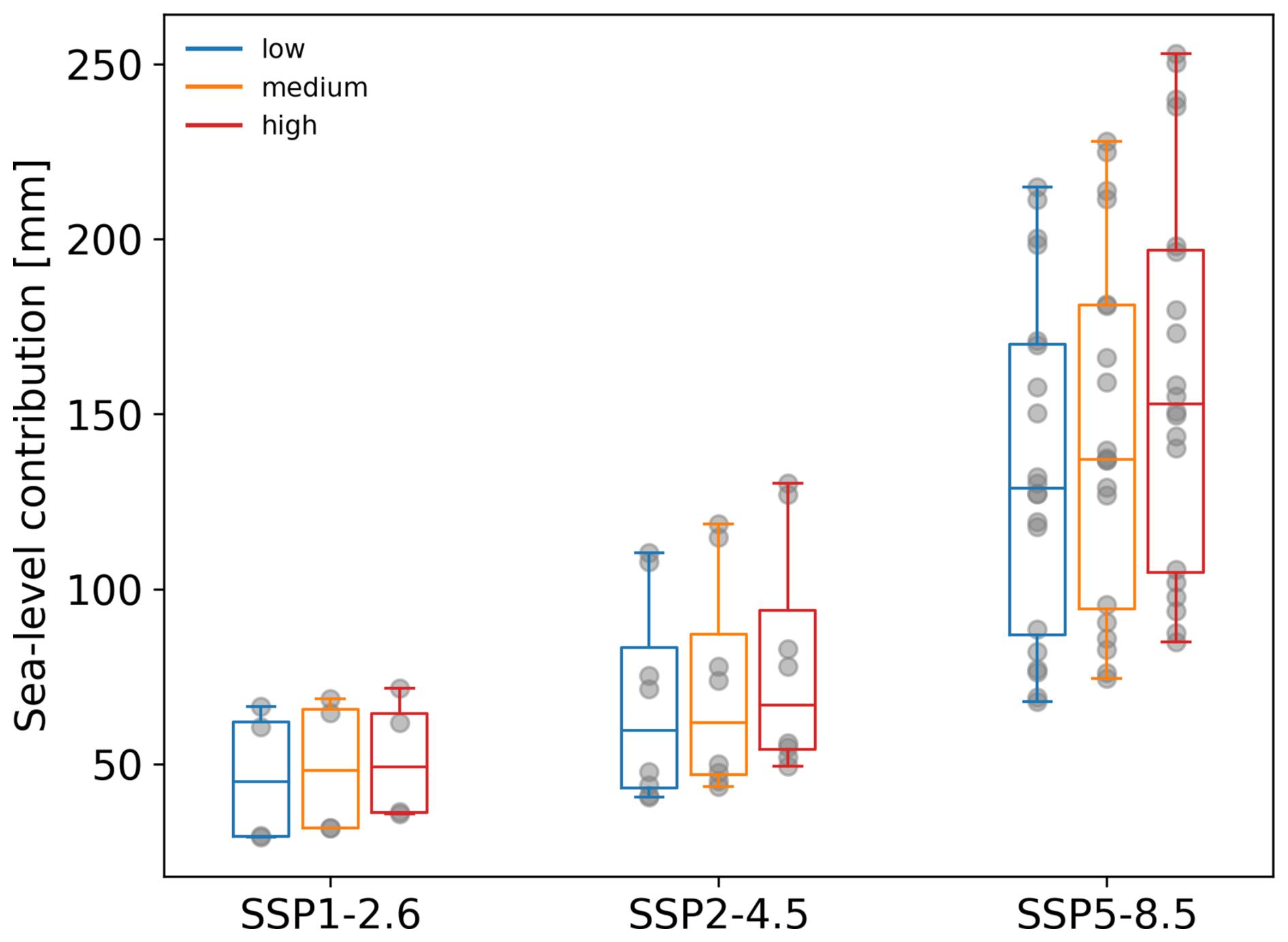
Figure 11 Projected sea-level contribution until 2100 for the entire ensemble, grouped by emission scenario. Colors denote sensitivity to outlet glacier retreat forcing. Grey dots represent the individual ESM projections, which include results for both initialization methods. Whiskers show the full range of values; horizontal lines denote the median.

Running each simulation at 16, 8, and 4 km grid resolution, we perform a grid sensitivity study for the ERA5-init ensemble. We compare the resulting sea-level contribution at 2100 of each simulation to their 4 km counterpart (Fig. 12). For the SSP1-2.6 scenario the mean absolute difference in simulations at 16 km resolution to simulations at 4 km resolution is 4.85 mm, with slight variations depending on the sensitivity to outlet glacier retreat forcing. The maximal deviation is 8.74 mm. Mean absolute deviations for the SSP2-4.5 (SSP5-8.5) scenario are similar, with a mean absolute of 3.79 mm (5.08 mm). While the maximal deviation for the SSP2-4.5 is 7.5 mm, the largest difference for the SSP5-8.5 scenario amounts to −12.28 mm, which is well below 10 % of the projected sea-level contribution.

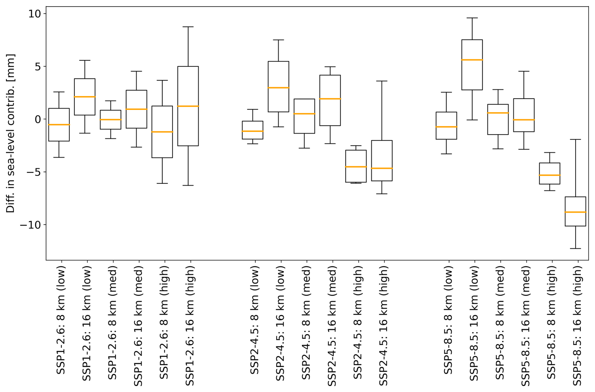
Figure 12 Difference in projected sea-level contribution in 2100 between simulations using different grid sizes. Shown is the difference in simulations run at 8 km (16 km) resolution to simulations run at 4 km resolution. Whiskers show the full range of values; orange lines denote the median.

4 Discussion and conclusions

In this study, we present ensemble projections of sea-level contribution from the Greenland ice sheet over the 21st century under three emission scenarios, using regionally downscaled forcing from various ESMs in the CMIP6 and CMIP5 archive. We examine the influence of the initialization forcing on projected sea-level contributions. Our projections, which include the response to historic climate forcing, suggest a sea-level contribution of 30 to 70 mm under the SSP1-2.6 scenario, 40 to 120 mm under the SSP2-4.5 scenario, and 70 to 230 mm under the SSP5-8.5 scenario. These results are consistent with recent studies that also use CMIP6 forcing (Hofer et al., 2020; Payne et al., 2021; Choi et al., 2021).

Uncertainty analysis of our ensemble shows that climate forcing is the largest source of uncertainty in the projected sea-level contribution. The spread of uncertainty due to climate forcing is 154 mm (corresponding to a 2σ range of 99 mm) for the SSP5-8.5 scenario, 75 mm (corresponding to a 2σ range of 58 mm) for SSP2-4.5, and 37 mm (corresponding to a 2σ range of 35 mm) for SSP1-2.6, with significant overlap across scenarios. This range is larger than the uncertainty due to ice sheet model formulations evaluated in the ISMIP6 study. Goelzer et al. (2020b) reported a spread of about 80 mm (2σ range) in projections forced with the Model for Interdisciplinary Research on Climate (MIROC5) under the RCP8.5 (Representative Concentration Pathway) scenario assuming medium sensitivity to retreat forcing, which is attributed due to differences between ice sheet models. This difference highlights the greater importance of climate forcing over specific model formulations and setups.

The uncertainty in SMB can largely be attributed to climate forcing uncertainty, as shown by previous studies (Holube et al., 2022). However, another significant uncertainty in projected sea-level contribution stems from the uncertainty in the parameterization for outlet glacier retreat, contributing up to 25 mm to the overall spread. While we find the initial state of the ice sheet (SMB, friction field, and ice sheet thickness) to have an impact on the projected mass loss, with an uncertainty well below 10 mm in the SSP5-8.5 projections, this impact remains small. Similarly, the impact of the grid resolution is minimal, with a mean absolute difference in sea-level contribution of below 5 mm across scenarios. This can be attributed to the near grid-size independent formulation of the outlet glacier retreat parameterization and the conservative interpolation of SMB forcing.

While many past studies have focused their attention on the two extreme ends of emission scenarios (SSP1-2.6 and SSP5-8.5), we succeed to close this gap in scenario uncertainty by including multiple projections for the intermediate SSP2-4.5 scenario. In light of current socioeconomic conditions, SSP2-4.5 might be a particularly realistic future pathway, and it is therefore important to increasingly sample projections for this or other intermediate scenarios.

Goelzer et al. (2020b) identified reducing inaccuracies in the initial state of the ice sheet as a critical priority for the ice sheet modeling community. Our initialized ice sheet configurations achieve RMSEs in ice sheet thickness (Fig. 1) that are comparable to the most accurate results from the ISMIP6 ensemble. Notably, in ISMIP6, a close match between the initial ice sheet geometry (or surface velocity) and observational data often resulted in significant model drift following initialization. In this study, we address this issue by presenting an improved initialization method, coupled with a historical run, that closely matches observations while minimizing model drift. This approach allows us to use the projections directly, without subtracting control runs, thereby incorporating short-term historical forcing effects and producing historically consistent projections. We view this as a significant advancement in the development of modeling frameworks for future ice sheet intercomparison projects. However, a limitation of the inversion method used in this study is the nonphysical transfer of uncertainties, such as those related to surface mass balance (SMB), geothermal heat flux, and model parameters, into the bed friction field. In the absence of accurate observational data on bedrock conditions beneath the ice, this drawback remains acceptable, given its limited impact on centennial timescales.

The ISMIP6 forcing approach used SMB anomalies to remove ESM and regional climate model (RCM) bias, creating an experimental setup suitable for ice sheet ensembles and intercomparisons. However, ISMIP6 also highlighted the need to explore a more consistent forcing approach that uses absolute SMB fields. In this study, we address this issue by comparing projections that use both SMB anomalies and the absolute SMB. We employ two simulation strategies: one initializes the ice sheet with an ESM-based SMB and then forces subsequent projections with absolute SMB from the ESM, and the other combines the baseline SMB used for initialization with SMB anomalies derived from the ESM. Since the anomalies are the same in both cases, the projections are directly comparable. Our results indicate little to no difference in the projected sea-level contribution between the two approaches, suggesting that the choice of using an SMB product from a reanalysis vs. SMB from an ESM for initialization does not significantly affect the uncertainty in the projections. This supports the suitability of a modeling framework that employs a common initialization and anomaly forcing for generating large ensembles of ice sheet projections, which is particularly valuable for community efforts like future intercomparison projects. Moreover, performing multiple spin-ups is computationally expensive, and most ESMs struggle to accurately reproduce the observed mean SMB over the reference period, even when downscaled, due to inherent biases (Vial et al., 2013). This can result in lower-quality initializations, highlighting the advantages of an anomaly-based approach for maintaining consistency across ensemble projections.

While our study uses forcing from multiple ESMs, we only consider one RCM, MAR, thereby neglecting RCM uncertainty. Given the significant role of SMB in future mass loss processes and discrepancies between different RCMs (Glaude et al., 2023), future studies should incorporate this uncertainty. Additionally, since only one ice sheet model is used, uncertainties due to model formulation, parameter choices, and modeling decisions are not fully represented.

To represent the retreat of marine-terminating outlet glaciers in response to ocean warming, we use a retreat parameterization, which is based on empirical data and is by design largely independent from model resolution. As demonstrated in this study, a coarser grid resolution (e.g., 16 km) proves to be sufficient, which is crucial when it comes to the efficient use of computational resources. This becomes relevant when running large ensembles of projections, for example, when sampling a wide range of climate forcing or when exploring parameter uncertainty. However, the drawback of the parameterization is its inability to resolve individual outlet glaciers and, in particular, fjord bathymetry. This inhibits the representation of small-scale processes in fjords and at the glacier front which are important drivers for the retreat of outlet glaciers. Future efforts are needed to improve on the representation of processes at the ocean–ice interface, especially with the prospect of accurate sea-level projections beyond 2100, when empirically derived relationships may no longer apply.

Appendix A

Table A1 Sea-level contributions for projections run at 4 km grid resolution. Listed are projections initialized with ERA5 (ESM) SMB. Low, med, and high denote the sensitivity to outlet glacier retreat forcing.