the Creative Commons Attribution 4.0 License.
the Creative Commons Attribution 4.0 License.
 | 12 Feb 2024
Snow water equivalent retrieval over Idaho – Part 1: Using Sentinel-1 repeat-pass interferometry
Shadi Oveisgharan
Robert Zinke
Zachary Hoppinen
Hans Peter Marshall
Snow water equivalent (SWE) is identified as the key element of the snowpack that impacts rivers' streamflow and water cycle. Both active and passive microwave remote sensing methods have been used to retrieve SWE, but there does not currently exist a SWE product that provides useful estimates in mountainous terrain. Active sensors provide higher-resolution observations, but the suitable radar frequencies and temporal repeat intervals have not been available until recently. Interferometric synthetic aperture radar (InSAR) has been shown to have the potential to estimate SWE change. In this study, we apply this technique to a long time series of 6 d temporal repeat Sentinel-1 C-band data from the 2020–2021 winter. The retrievals show statistically significant correlations both temporally and spatially with independent in situ measurements of SWE. The SWE change measurements vary between −5.3 and 9.4 cm over the entire time series and all the in situ stations. The Pearson correlation and RMSE between retrieved SWE change observations and in situ stations measurements are 0.8 and 0.93 cm, respectively. The total retrieved SWE in the entire 2020–2021 time series shows an SWE error of less than 2 cm for the nine in situ stations in the scene. Additionally, the retrieved SWE using Sentinel-1 data is well correlated with lidar snow depth data, with correlation of more than 0.47. Low temporal coherence is identified as the main reason for degrading the performance of SWE retrieval using InSAR data. We also show that the performance of the phase unwrapping algorithm degrades in regions with low temporal coherence. A higher frequency such as L-band improves the temporal coherence and SWE ambiguity. SWE retrieval using C-band Sentinel-1 data is shown to be successful, but faster revisit is required to avoid low temporal coherence. Global SWE retrieval using radar interferometry will have a great opportunity with the upcoming L-band 12 d repeat-pass NASA-ISRO Synthetic Aperture Radar (NISAR) data and the future 6 d repeat-pass Radar Observing System for Europe in L-band (ROSE-L) data.
- Article
(13677 KB) - Full-text XML
- Companion paper
- BibTeX
- EndNote


© 2024 California Institute of Technology. Government sponsorship acknowledged.
The seasonal snowpack provides water resources to billions of people worldwide (Barnett et al., 2005). Snow is the primary source of water for river channel discharge in middle-to-high-latitude areas. Therefore, snow mass and snow cover has a great impact on global and regional water cycles. Large-scale mapping of snow water equivalent (SWE) with high resolution is critical for many scientific and economics fields. SWE is defined as the depth of water which would be obtained if all ice contained in the snowpack were melted. NASA SnowEx is a multi-year effort to improve SWE and snow surface energy balance measurements and estimates. SWE has been identified as the key variable for terrestrial snow by the SnowEx campaign and NASA's decadal survey.
Estimating SWE on a global scale with enough accuracy and resolution is still a challenge. Passive spaceborne sensors based on the microwave emission of the snowpack (Takala et al., 2011; Kelly et al., 2003; Pulliainen and Hallikainen, 2001; Kelly, 2009) have a coarse spatial resolution on the 10 km scale. The technique saturates for SWE deeper than 150 mm, which makes their application in the mountains challenging. Nevertheless, passive microwave sensors represent the current state of the art of SWE retrieval methods. These sensors are applied operationally to generate daily estimates of SWE globally (Takala et al., 2011; Kelly et al., 2003); however, many products such as GlobSnow mask out mountainous areas, due to the saturation limit and resolution.
Airborne lidar has been successful in estimating snow depth (Painter et al., 2016). However, clouds and limited regional coverage are limiting factors for this method. This technique also needs a snow-density model to estimate SWE from the lidar snow depth, and there currently is not a path to space for global snow depth mapping at the temporal resolution required.
Active microwave sensors provide high-resolution and global coverage. There have been many efforts in the last 2 decades trying to estimate SWE or snow depth using active sensors mounted on a tower (Cui et al., 2016; Lemmetyinen et al., 2018; Ruiz et al., 2022; Leinss et al., 2015), airborne (Marshall et al., 2021; Nagler et al., 2022), or spaceborne systems (Lievens et al., 2019; Liu et al., 2017; Conde et al., 2019; Dagurova et al., 2020; Eppler et al., 2022). Backscattered power from active sensors is used to estimate SWE (Rott et al., 2010; Ulaby and Stiles, 1980; Cui et al., 2016; Nghiem and Tsai, 2001; Lievens et al., 2019). A dual-band (X and Ku) SAR mission has been the focus of the European Space Agency (ESA) and Canadian Space Agency (CSA) for SWE spaceborne measurements (Rott et al., 2010; Lemmetyinen et al., 2018). However, accurate a priori characterization of snow micro-structural parameters is of primary importance in the accuracy of SWE retrieval algorithms using backscattered power (Lemmetyinen et al., 2018; Durand and Liu, 2012; Cui et al., 2016). The most common a priori characterization used for SWE retrieval algorithms using backscattered power is grain radius. This has been done using passive data; however, the methods are limited by passive retrieval errors and also mismatch between active and passive resolutions. The ratio of cross-polarized to co-polarized Sentinel-1 backscattered power has been used to estimate snow depth over mountainous regions with deep snow (Lievens et al., 2019, 2022). Using Sentinel-1 backscattered power ratio is a unique approach showing the success of snow depth retrieval using the spaceborne radar time series data. However, the retrieval mostly works for deep snow in mountainous regions. The radiative transfer physics at C-band for this method are still poorly understood. The co-polar phase difference (CPD) between VV and HH polarization of X-band SAR acquisitions is used for estimating the depth of fresh snow (Leinss et al., 2014).
Lightweight and portable frequency-modulated continuous-wave (FMCW) radar systems have been used to map snowpack properties (such as depth, SWE, and stratigraphy) rapidly over large distances and at high resolution (Marshall and Koh, 2008). The system was normally deployed nadir looking and was a real aperture radar system. The resolution of FMCW system for SWE application is in centimeter scale. In order to achieve such high resolution, the bandwidth should be in gigahertz scale. Due to limitation on frequency bandwidth allocation of a spaceborne active sensor (Tao et al., 2019), FMCW systems cannot be used in spaceborne missions for global coverage due to their wide bandwidth.
The phase change of specularly reflected signals in signals of opportunity (SoOp) is shown to be strongly dependent on SWE changes for dry snow (Yueh et al., 2017, 2021; Shah et al., 2017). The theory behind using SoOp for SWE retrieval is similar to repeat-pass interferometry that is explained in Sect. 2. The advantage of this method is that the stratigraphy of the snow has little impact on the SWE retrieval (Leinss et al., 2015; Yueh et al., 2017), similar to SWE retrieval explained in Sect. 2. Using the long wavelength signal at P-band in SoOp is very helpful for addressing the loss of temporal coherence and phase unwrapping challenges of this method. However, the phase sensitivity to SWE changes decreases at lower frequencies. There have been very limited data showing the success of this method at P-band. Achieving high resolution for SoOp data is another challenge (Yueh et al., 2017, 2021; Shah et al., 2017).
As explained in detail in next section, the phase difference between two SAR observations is proportional to changes in SWE variation (ΔSWE). We evaluated the performance of SWE retrieval using interferometry over Idaho. In Part 1 of this study (the current paper), we used Sentinel-1 interferometric time series data over Idaho. In Part 2 (Hoppinen et al., 2024), we use Uninhabited Aerial Vehicle Synthetic Aperture Radar (UAVSAR) interferometric time series data over Idaho to evaluate the performance of this method. We explain SWE estimation using repeat-pass interferometry in Sect. 2. The details about different data sets used in this study are discussed in Sect. 3. Section 4 describes how we processed Sentinel-1 data and convert them to SWE. The retrieved SWE is compared with in situ and lidar data in Sect. 5. This work shows the success of SWE retrieval using long-time-series spaceborne InSAR data in winter 2021.
Differential SAR interferometry measurements have been used to detect small surface elevation changes over large areas with a vertical accuracy of a few millimeters (Gabriel et al., 1989; Zebker et al., 1994). The measured phase difference is proportional and sensitive to changes in SWE variation (ΔSWE) during the snow season (Guneriussen et al., 2001; H. Rott and Scheiber, 2003; Deeb et al., 2011; Leinss et al., 2015; Conde et al., 2019; Liu et al., 2017; Hui et al., 2016; Nagler et al., 2022; Eppler et al., 2022; Dagurova et al., 2020; Marshall et al., 2021). The main advantage of this method is its simplicity and a reduction in necessary a priori information.
The snow volume scattering affects the interferometric phase for very deep snow in Greenland at relatively high frequencies such as C-band (Oveisgharan and Zebker, 2007). However, for the terrestrial snow, the effect of volume scattering of dry snow on the interferometric phase is very small compared to scattering from the ground at high frequencies. The snow refractive index delays the echo received from the ground. The signal delay caused by refraction can be measured with differential radar interferometry as (Guneriussen et al., 2001; Leinss et al., 2015)
where , and ϵ are the interferometric phase between two observation dates, incidence wavenumber, snow depth change, incidence angle, and permittivity of the snow, respectively. The change in the interferometric phase is used to calculate ΔSWE (Leinss et al., 2015; Conde et al., 2019; Liu et al., 2017; Nagler et al., 2022). Similar to the dual-polarization, dual-frequency retrieval algorithm (Lemmetyinen et al., 2018; Cui et al., 2016), this technique relies on the dryness of snow in order to penetrate all the way to the ground so that the scattering from the snow layers and snow volume is minimized compared to the snow–ground return (Oveisgharan et al., 2020).
Using Envisat interferometric data to estimate SWE was not very successful mainly due to the large temporal baseline and, hence, low temporal coherence (Hui et al., 2016). A modified version of SWE estimation using InSAR is also introduced (Eppler et al., 2022; Dagurova et al., 2020). The backscattering from the roughness in the ground and snow layers is combined with the interferometric phase to improve the accuracy (Dagurova et al., 2020). The sensitivity of the dry-snow refraction-induced InSAR phase to topographic variations is used to bypass the unwrapping problem (Eppler et al., 2022). Airborne data collected over the Austrian Alps in 2021 showed good agreement between retrieved SWE using InSAR and mean in situ SWE. Root mean square differences of 4.0 mm for a small snowstorm of 14 mm snow depth at C-band and 11.2 mm for a big snowstorm of 66 mm at L-band were observed (Nagler et al., 2022). The correlation of 0.76 was observed between the retrieved SWE change using L-band UAVSAR differential interferometry between 1 and 13 February 2020 and the collected lidar snow depth change between 1 and 12 February 2020 over the open regions of Grand Mesa in dry-snow conditions (Marshall et al., 2021). SWE retrieval using Sentinel-1 interferometric data showed a mean accuracy of 6 mm over Finland for just two passes (Conde et al., 2019).
All these studies have proven the potential of this method but were limited in time or space for data collection or validation. In this study, we show the performance of SWE retrieval using a long time series of Sentinel-1 interferometric data in winter 2021. This study shows that SWE estimation using repeat-pass interferometry works well by validating the retrieved value with a large number of in situ stations and two regional lidar snow depth maps.
With the recent SnowEx 2020 campaign using UAVSAR L-band differential interferometry data, Sentinel-1 C-band differential interferometry, and future NASA-ISRO SAR (NISAR) L-band data, there will be more advances in the limitations and capabilities of this method.
2.1 Temporal coherence
The received radar signals at two different times will be correlated with each other if the set of scatterers in the resolution cell remain the same. However, the movement of the scatterers such as leaves and branches or sea ice particles decreases the temporal coherence (Zebker and Villasenor, 1992; Kellndorfer et al., 2022; Lavalle et al., 2012). The loss of coherence between the observations is one of the main limitations for SWE retrieval using differential interferometry. Methods such as using two frequencies or shorter revisit time are used to overcome these problems (Deeb et al., 2011; Leinss et al., 2015). Melting and wind are the main reasons for low temporal coherence in snow (Leinss et al., 2015; Luzi et al., 2009). A medium mean temporal coherence of 0.41 is observed at L-band between two winter seasons in shrub-lands with 10.2 cm average snow depth (Molan et al., 2018). Temporal coherence decreases with increasing frequency (Leinss et al., 2015; Nagler et al., 2022; Kellndorfer et al., 2022; Ruiz et al., 2022). A median temporal coherence of about 0.5 is observed at 10.2 and 16.8 GHz even after 60 d (Leinss et al., 2015). However, the spaceborne TerraSAR-X temporal coherence over snow at 9.65 GHz is reduced significantly in 11 d (Leinss et al., 2015). This is probably due to random phase drifts over time that cannot be estimated and corrected in a spaceborne system compared to a ground radar. Vegetation cover decreases the temporal coherence significantly at high frequencies (Baduge et al., 2016; Kellndorfer et al., 2022; Ruiz et al., 2022). A tower-based fully polarimetric InSAR studied the effect of air temperature, precipitation intensity, and wind on the temporal decorrelation at L-, S-, C-, and X-bands (Ruiz et al., 2022). The temperature was shown to be the most critical variable affecting the temporal coherence among other variables. Temperature above 0 ∘C reduced the temporal coherence drastically (Ruiz et al., 2022). On the other hand, snow cover has a thermal insulation effect on the ground and underlaying layers (Gu et al., 2019). The insulation increases with the snow depth. Therefore, during the snow season we assume the ground remains frozen even when snow becomes wet. Hence, temporal decoherence from the ground is negligible. SWE accumulation retrieval was successful for short temporal baselines and low frequencies in non-vegetated areas. However, the error increased for high frequencies and long temporal baselines. The SWE profile retrieval using C-band data performs well using 12 h and 1 d repeat-pass data. The retrieval is poor using the 12 d repeat-pass data at C-band (Ruiz et al., 2022). The 6 d repeat-pass C-band data showed good performance for small SWE changes but poor performance for large SWE changes between the interferometric pairs due to phase ambiguity caused by large SWE change (Ruiz et al., 2022). The low temporal coherence and low penetration depth at frequencies higher than 10 GHz make L- and C-band desirable frequencies for differential interferometry.
2.2 Relationship between ΔSWE and Δϕ
With some approximation to Eq. (1), Leinss et al. (2015) showed a linear relationship between the interferometric phase and SWE change. The approximation is limited to a smaller range of incidence angle than Sentinel-1 incidence angle. However, Leinss et al. (2015) approximation applies to a wide range of snow density up to solid ice density. Due to the wide range of Sentinel-1 incidence angle in a frame, we tried to make a more accurate approximation for a wider range of incidence angles and snow densities limited to terrestrial snow. The snow permittivity in Eq. (1) is dependent on snow density, ρ (g cm−3), and relatively independent of signal wavelength. Following Leinss et al. (2015), we use Mätzler's model (Mätzler, 1987) for calculating ϵ in Eq. (1) ( for ρ<0.4 g cm−3; and for ρ>=0.4 g cm−3). We can rewrite Eq. (1) as
where . Note that ϵ(ρ) and consequently C(θ,ρ) are unitless, ρwater=1 g cm−3, ΔSWE is in meters (m), and κi is in per meter (m−1).
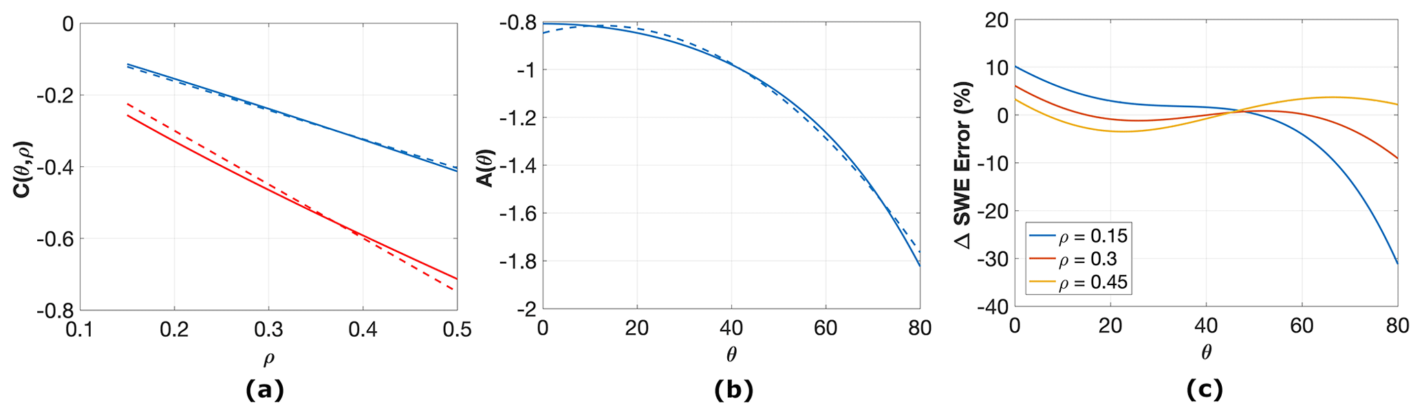
Figure 1(a) C(θ,ρ) versus snow density for θ=0 and θ=70 shown by solid blue and red lines, respectively. The blue and red dashed lines show the linear fit to C(θ,ρ) with zero intercept . (b) The line slope in panel (a) versus incidence angle. The dashed line shows the fitted polynomial, . (c) ΔSWE error percentage (), assuming versus incidence angle for snow density equal to 0.15, 0.3, and 0.45 g cm−3, shown by blue, red, and yellow lines, respectively.
The blue and red lines in Fig. 1a show C(θ,ρ) versus snow density for incidence angles equal to 0 and 70∘, respectively. As seen in this figure, there is approximately a linear relationship between C and snow density. We fit a line to C for different incidence angles as for g cm−3. The blue and red dashed lines show at incidence angles equal to 0 and 70, respectively. As seen in Fig. 1a, the fitted line with zero intercept is a good approximation. The zero intercept approximation is essential to retrieve ΔSWE independent of snow density. The incidence angle mostly lies between 0 and 80 for Sentinel-1 data. The terrestrial snow density lies mostly between 0.15 and 0.5 g cm−3. Therefore, we limit ourselves to incidence angle between 0 and 80 and snow density between 0.15 and 0.45 g cm−3 in fitting a line to C. Solid blue line in Fig. 1b shows A(θ) versus incidence angle. By fitting a polynomial to A, we can write it as
The dashed blue line in Fig. 1b shows the fitted curve, . We can rewrite Eq. (1) as
Figure 1c shows the versus incidence angle for different snow densities. As seen in this figure, the error in ΔSWE calculation using the approximation in Eq. (4) is less than 10 % for incidence angles less than 70. We use Eq. (4) for estimating ΔSWE using the interferometric phase, Δϕ, for the rest of this study. Using one equation for the entire Sentinel-1 frame makes the interferometric phase conversion to ΔSWE very convenient. However, we need to keep in mind that the approximation for lower-density snow has more than 10 % error for an incidence angle larger than 70.
3.1 Sentinel-1
The Sentinel-1 radar operates at C-band at a central frequency of 5.405 GHz. It has four exclusive imaging modes with different resolutions (down to 5 m) and swath width up to 400 km. Sentinel-1 has dual-polarization capability and rapid product delivery. The Sentinel-1 constellation includes Sentinel-1A and Sentinel-1B. These two satellites are in the same orbit, with a 180∘ orbital phasing difference. The revisit time for each of the satellites is 12 d. However, revisit time can get to 6 d if both satellites make observations. The data are free and available through the Alaska SAR Facility (ASF) or the Copernicus Data Hub distribution service. We used the Interferometric Wide (IW) swath mode data with 5 and 20 m single-look resolution in the range and azimuth direction, respectively. The IW swath width is about 250 km. We used ASF on-demand processing to generate the interferometric phase and coherence at vv and vh (transmit-received polarization) polarization. The Alaska Satellite Facility's Hybrid Pluggable Processing Pipeline (HyP3) is a service for processing synthetic aperture radar (SAR) imagery (Hogenson et al., 2020). The workflow includes interferometric phase correction for ground topography and geolocation. The ASF HyP3 uses a minimum cost flow (MCF) algorithm for phase unwrapping. The unwrapped phase and interferometric coherence were used in this study. The resolution of the HyP3 phase and coherence is 80 m × 80 m. Sentinel-1 collects data every 12 d globally but has the capability to collect the data every 6 d over targeted areas, mainly over Europe and selected areas such as SnowEx sites. In order to validate our SWE retrieval using Sentinel-1 data, we use lidar data from the SnowEx campaign and SNOwpack TELemetry Network (SNOTEL) data as discussed in Sect. 5. We also use the average of SNOTEL data as a reference point for SWE retrieval, as seen in Sect. 4.
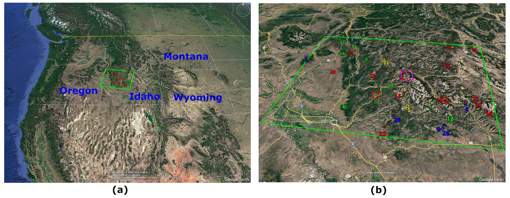
Figure 2© Google Earth View. (a) Google Earth View of Sentinel-1 path 71, frame 444, in Idaho. (b) Zoomed to the Sentinel-1 path 71, frame 444, shown by the big green rectangle. Red boxes show the location of lidar data acquisition. The green diamonds show SNOTEL stations with an ΔSWE error of less than 2 cm in the entire time series. The red diamonds show SNOTEL stations with an ΔSWE error of more than 2 cm in at least one observation in the time series. Yellow squares are SNOTEL stations 1 and 11 used are a reference point. Blue diamonds show the location of stations with temporal coherence less than 0.35 or temperature more than 0 ∘C in the entire time series.
The NASA SnowEx 2021 time series is the continuation of the multi-year effort to improve SWE measurements and estimates. The data acquisition for different sensors and in situ collections spread over different US sites in winter 2020. These sites span a range of snow climates and conditions, elevations, aspects, and vegetation. Flight paths were designed to include sites with ongoing snow research projects, existing ground-based remote sensing infrastructure (e.g., radar and lidar), snow-off and planned snow-on aerial lidar, and scheduled ground snow measurement. The 2021 time series data set covers fewer regional sites and more frequent temporal sampling compared to the 2020 campaign. The SnowEx campaign coordinated with the Sentinel-1 team to observe some of the SnowEx sites with 6 d revisit during the winter, which included the Idaho SnowEx sites.
Figure 2a shows one of these sites that was observed every 6 d with Sentinel-1 over Idaho. The green frame shows the geographic location of path 71, frame 444, of Sentinel-1 data. Figure 2b is zoomed to the Sentinel-1 frame in panel (a).
3.2 SNOTEL
SNOwpack TELemetry Network (SNOTEL) sites are located in remote, high-elevation mountainous regions in the western US. They automatically measure different snowpack characteristics and climate conditions. We used the United States Department of Agriculture (USDA) website to access hourly SNOTEL data (https://wcc.sc.egov.usda.gov/nwcc/inventory, last access: August 2023) over the region of interest shown in Fig. 2b. As the Sentinel-1 frame in Idaho is collected at around 06:00 local time, we downloaded the SWE, snow depth, and near-surface air temperature at 06:00 for each of the SNOTEL stations. Small red, green, and blue diamonds in Fig. 2b show the SNOTEL locations in the Sentinel-1 frame. Figure 3a shows the time series SWE of these SNOTEL sites starting from 1 December 2020 at 06:00. Different colors show different SNOTEL stations. The elevation of these stations varies between 975 and 2902 m. Therefore, the large spread of SWE between different stations in Fig. 3a is expected. The dashed vertical lines are the start date of each 6 d repeat Sentinel-1 data. As seen in this figure, there is a 6 d repeat data acquisition gap in Sentinel-1 data on 5 February 2021. Figure 3b shows the mean ± standard deviation (SD) of SNOTEL ΔSWE between the start date Sentinel-1 data in Fig. 3a and 6 d later. We used the SWE data from these in situ stations for (a) SWE retrieval validation by comparing retrieved ΔSWE with SNOTEL ΔSWE (as seen in Sect. 5.1) and (b) the InSAR reference point by subtracting the average of two SNOTEL ΔSWE from the retrieved ΔSWE (as explained in Sect. 4).
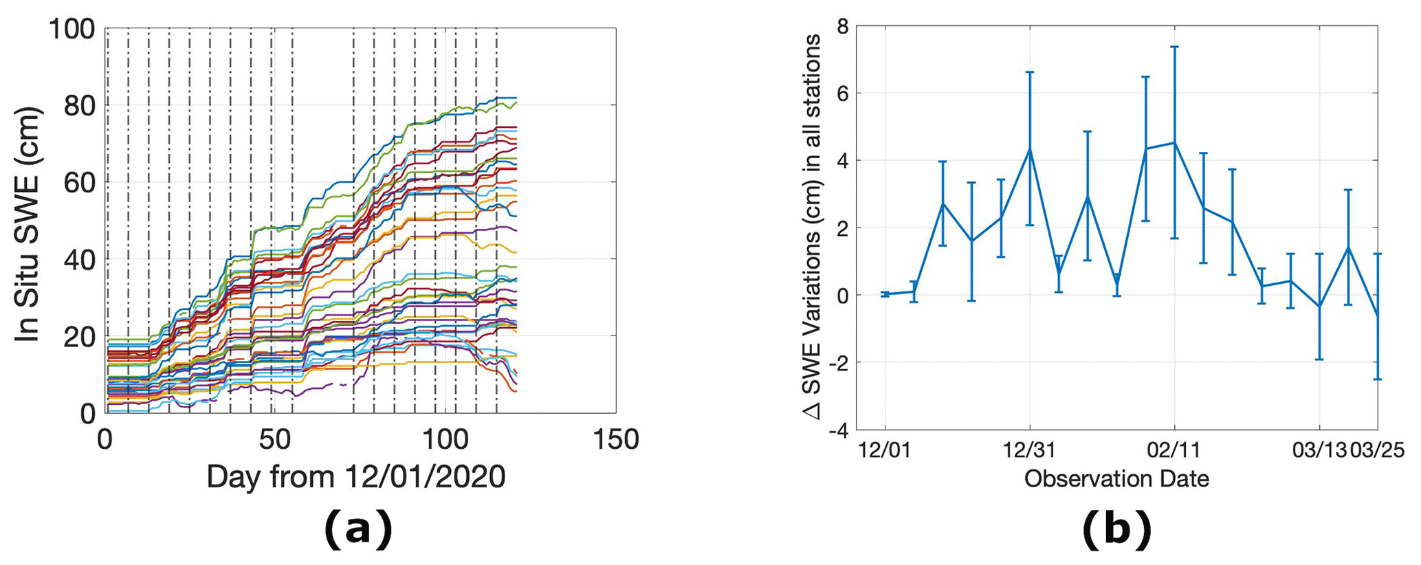
Figure 3(a) The daily SWE (cm) of in situ stations shown in Fig. 2b from 1 December 2020 to 30 March 2021. The dashed vertical lines show the start date of Sentinel-1 observations. (b) The mean ± SD of in situ ΔSWE for Sentinel-1 observation dates shown in panel (a). Note that the ΔSWE is marked on the first day of each observation.
3.3 QSI lidar
Airborne lidar provides high-resolution snow depth maps. These data are reliable sources of validation data and a particularly powerful constraint for InSAR retrieval of SWE. We used the lidar data for validating the retrieved SWE results. The “SnowEx20-21 QSI Lidar DEM 0.5m” data set is part of the SnowEx 2020 and SnowEx 2021 campaigns (Adebisi et al., 2022). The data include digital elevation models, snow depth, and vegetation height with 0.5 m spatial resolution. Data were acquired over multiple areas in Colorado, Idaho, and Utah during February 2020, March 2021, and September 2021. The two red boxes in Fig. 2b show the location of lidar data acquisition. The big purple box is over Banner Summit and the small red box is over Mores Creek in Idaho. Figures 10a and 11a show the QSI snow depth over Banner Summit and Mores Creek, respectively. We used these data in Sect. 5.2 to compare with retrieved SWE using Sentinel-1 data.
As mentioned in Sect. 3.1, Sentinel-1 data were collected every 6 d over the region shown in Fig. 2b during 2020 and 2021, following coordination between the SnowEx campaign and the Sentinel-1 team. We used 6 d repeat Sentinel-1 time series data between 1 December 2020 and 30 March 2021. We selected this period to (a) capture most of the seasonal snowstorm and (b) avoid wet snow as much as possible. The main sources of error in the science and applications using Sentinel-1 repeat-pass interferometry are (1) tropospheric noise, (2) temporal decorrelation, and (3) phase ambiguity. We removed tropospheric noise from the unwrapped phase as explained in Sect. 4.1. The unwrapped phase is converted to ΔSWE using Eq. (4). Temporal decorrelation is relatively high at C-band. The 6 d repeat time improves the temporal coherence significantly over snow compared to the normal 12 d Sentinel-1 repeat time. In this study, any pixel with temporal coherence more than 0.35 is considered reliable. Temporal coherence of 0.35 is arbitrary, but based on experience working with InSAR data, it is a reasonable threshold number. However, for the results in Sect. 5.2, we used all the time series data, including the data with low coherence, to calculate total SWE. The reason is that in order to compare the total SWE on a date close to the lidar acquisition date, we need the whole ΔSWE time series up to that date.
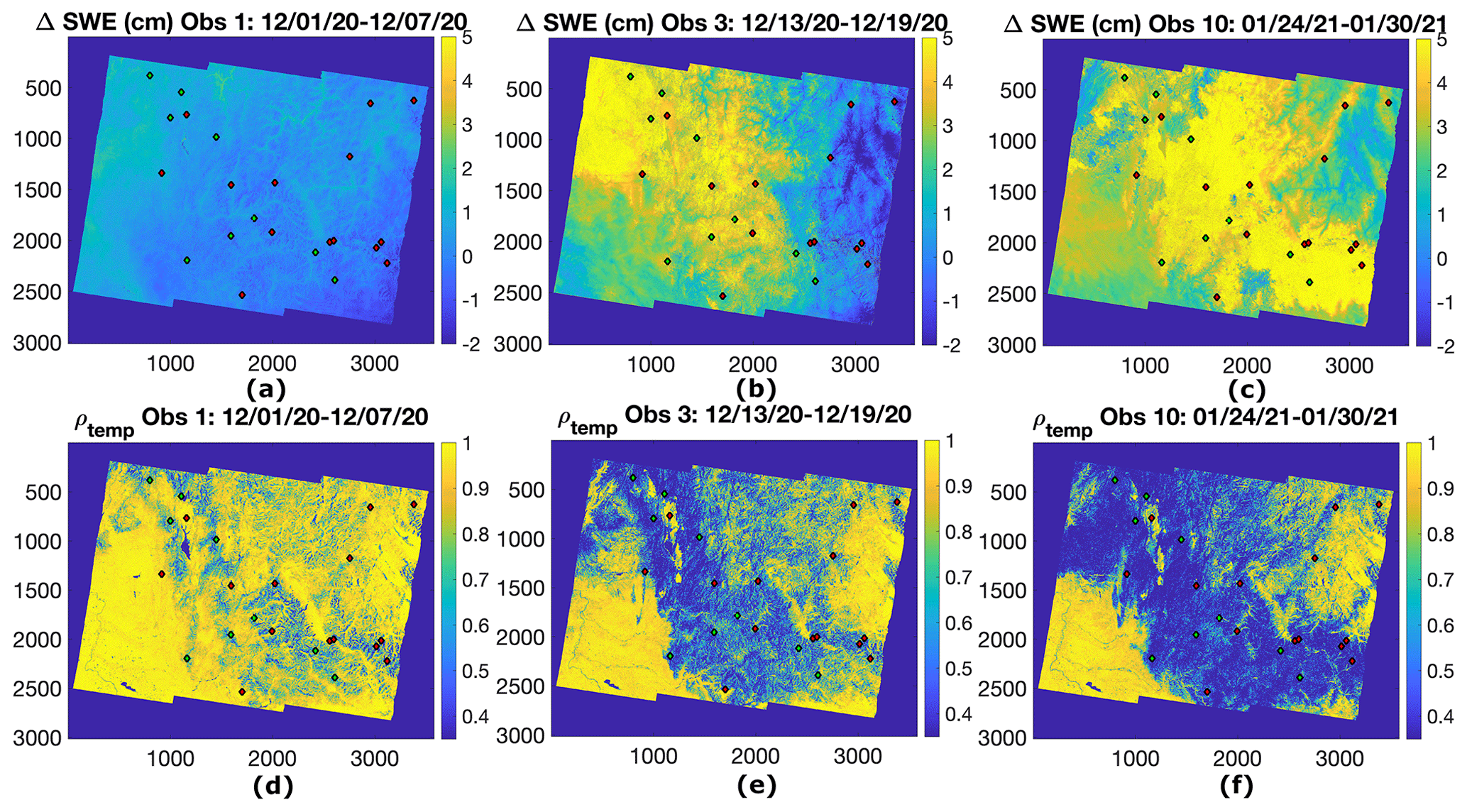
Figure 4Retrieved ΔSWE using Sentinel-1 path 71, frame 444, interferometric phase data between (a) 1 and 7 December 2020, (b) 13 and 19 December 2020, and (c) 24 and 30 January 2021. Sentinel-1 path 71, frame 444, coherence between (d) 1 and 7 December 2020 (observation 1), (e) 13 and 19 December 2020 (observation 3), and (f) 24 and 30 January 2021 (observation 10). The small diamonds are in situ locations. The averages of in situ ΔSWE for panels (a), (b), and (c) are 0.01, 2.72, and 4.33 cm, respectively.
Phase ambiguity is still one of the big sources of error in some of our data as discussed in Sect. 5.1.2. The radar signal propagating through the ionosphere is delayed. The delay is a function of frequency of the signal, Earth's magnetic field, and total electron content (TEC) and affects the accuracy of the ΔSWE retrieval. The ionospheric error at C-band is much smaller than other sources of error, and we consider it negligible in this study.
The temperature is also an important factor. Equation (1) is valid for dry snow (Leinss et al., 2015), and we use near-surface air temperature above 0 ∘C as a metric that indicates wet snow in the snow season. Any retrieved SWE with SNOTEL near-surface air temperature more than 0 ∘C is unreliable in our study. Similar to coherence filtering, for the results in Sect. 5.2, we used all the time series data, including the data with temperature more than 0 ∘C. Similar to temporal coherence, the reason is that in order to compare the total SWE with lidar snow depth on the lidar acquisition date, we need the entire ΔSWE time series up to that date.
Another important factor in interferometric phase images is the reference point to calibrate the unwrapped phase or consequently ΔSWE. In geophysics applications using InSAR, the reference point is a stable target with no displacement or known displacement in the time interval between acquisition of the two images. For ΔSWE estimation using InSAR, the reference point is chosen either by corner reflectors (cleaned of snow) with stable zero phase (Nagler et al., 2022; Dagurova et al., 2020) or using the average of in situ ΔSWE (Conde et al., 2019) or using a snow-free region (Tarricone et al., 2023). As seen in Fig. 2b, there are a large number of in situ stations in this frame. In this study, we used the average of two in situ ΔSWE values to calibrate the retrieved ΔSWE images. The two selected in situ stations have reliable measurements (coherence more than 0.35 and temperature less than 0 ∘C) for the entire time series. For the rest of this study we used in situ stations 1 and 11 ΔSWE values to calibrate the retrieved ΔSWE. Stations 1 and 11 are shown by yellow squares in Fig. 2b.
Figure 4a, b, and c show retrieved ΔSWE between 1 and 7 December 2020, 13 and 19 December 2020, and 24 and 30 January 2021, respectively. The small diamonds show the location of in situ stations in this Sentinel-1 frame. The averages of in situ ΔSWE for Fig. 4a, b, and c are 0.01, 2.72, and 4.33 cm, respectively. The retrieved ΔSWE images in the top row of Fig. 4 show no SWE change in panel (a) and snowstorms in panels (b) and (c), which match the in situ measurements.
The bottom row of Fig. 4 shows the coherence of the images in the top row of Fig. 4. Interferometric decorrelation has different sources, such as temporal decorrelation, volume decorrelation, signal to noise ratio decorrelation, and geometric decorrelation, among others. The volume decorrelation is negligible due to the relatively small Sentinel-1 perpendicular baseline. Temporal decorrelation is the dominant source of decorrelation. For the rest of this study, we assume the observed interferometric decorrelation is approximately the temporal coherence. As shown in Fig. 4e and f, snowstorms reduce the coherence significantly, whereas no SWE change shows a very small decorrelation, as expected.
4.1 Tropospheric noise removal
A radio wave's differential phase delay variation through the troposphere is one of the largest error sources in interferometric synthetic aperture radar (InSAR) measurements, and water vapor variability in the troposphere is known to be the dominant factor. The differential delay present in a given interferogram may reach tens of centimeters. Various ways of mitigating tropospheric effects are routinely employed. Here, we used a global atmospheric weather model to predict the radar phase delay due to variations in atmospheric pressure and water vapor content between passes. Specifically, we used the European Center for Medium-Range Weather Forecasts (ECMWF) ERA5 model of atmospheric variables, which provides hourly estimates on a 30 km global grid based on assimilation of surface and satellite meteorological data. We used the Python-based Atmospheric Phase Screen (PyAPS) software (Jolivet et al., 2011) to interpolate this grid and convert those variables into a radar phase delay. PyAPS is integrated into, and leveraged by, the Miami InSAR Time-series software in Python (MintPy) (Yunjun et al., 2019). We used MintPy to crop the atmospheric delays to match the spatial extent of the interferograms and projected the delays into radar line of sight (LOS). It should be noted that while the ERA weather models often provide a reliable method for representing atmospheric phenomena at >30 km wavelengths (grid spacing), they are less accurate at finer spatial scales, where atmospheric conditions can vary as a function of topography. Model interpolation between grid nodes as a function of elevation were performed; however, some over-smoothing of atmospheric variations might still occur. More work is necessary to better determine the overall effectiveness of atmospheric phase removal, including whether tropospheric delay is completely mitigated or overcorrected and on what spatial scales.
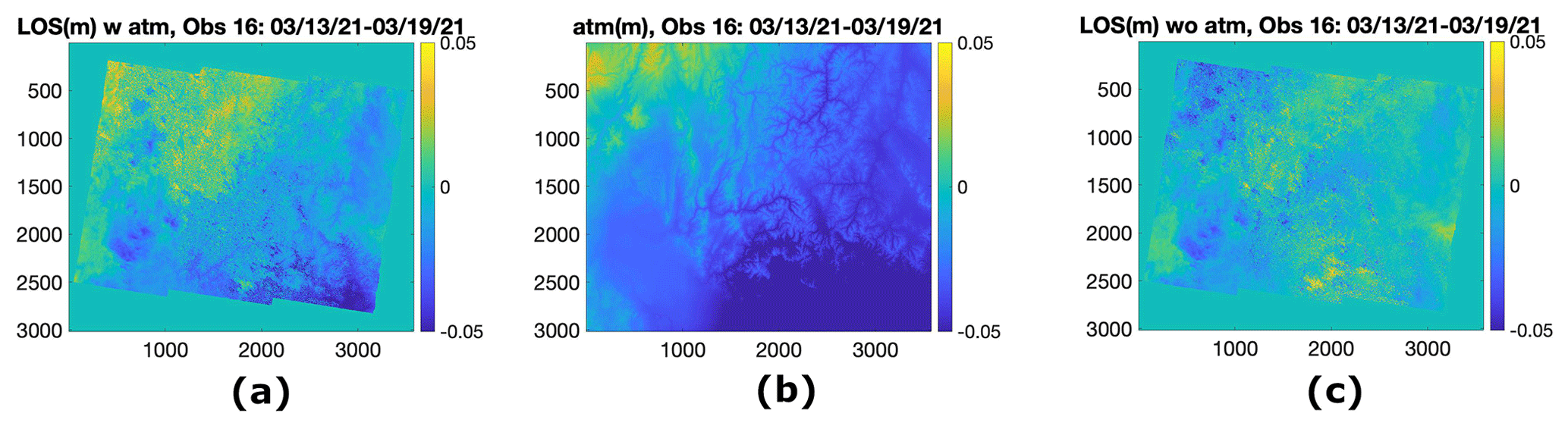
Figure 5Sentinel-1 path 71, frame 444, (a) line-of-sight (LOS) displacement (m) with atmospheric noise, (b) atmospheric noise (m), and (c) line-of-sight displacement (m) without atmospheric noise, between 13 and 19 March 2021.
Figure 5 shows an example of how significant tropospheric noise can be in an InSAR image. Figure 5a shows the line-of-sight displacement with no atmospheric correction over our area of interest in Fig. 2b between 13 and 19 March2021. Figure 5b shows the atmospheric noise estimation using PyAPS. Figure 5c shows LOS displacement after tropospheric noise removal by subtracting panel (b) from panel (a). Comparing Fig. 5a and c, we can see that the atmospheric noise can affect the estimated ΔSWE by 5–10 cm (LOS displacement error converted to ΔSWE) in the upper left of the images.
In this section we compare retrieved SWE using the Sentinel-1 interferometric phase with in situ stations and lidar data.
5.1 Comparing retrieved SWE using Sentinel-1 and SNOTEL SWE
5.1.1 Comparing retrieved ΔSWE using Sentinel-1 and SNOTEL ΔSWE
We used all the retrieved ΔSWE (using the Sentinel-1 data from 1 December 2020 to 30 March 2021) for in situ stations shown in Fig. 2b and compared them with corresponding SNOTEL ΔSWE. As mentioned in Sect. 4, any retrieved value with temporal coherence less than 0.35 and temperature higher than 0 ∘C is discarded. Note that the data shown in Fig. 6 are the SWE change between two consecutive Sentinel-1 data that are 6 d apart. We showed the ΔSWE for all stations and all consecutive observations between 11 December 2020 and 30 March 2021. As mentioned in Sect. 3.1, the resolution of the Sentinel-1 InSAR data from HyP3 is 80 m × 80 m. We used a 10×10 multi-look window of retrieved SWE and temporal coherence around the SNOTEL locations to reduce the speckle noise. Therefore, we compared the SNOTEL SWE with the 800 m × 800 m retrieved SWE around the SNOTEL site. The heterogeneity of the environment such as vegetation cover, vegetation fraction, land type, and SWE distribution in the 800 m × 800 m around the SNOTEL station affects our accuracy. We will analyze the effect of the heterogeneity of the environment on the SWE retrieval for SNOTEL stations in the future work of this study.
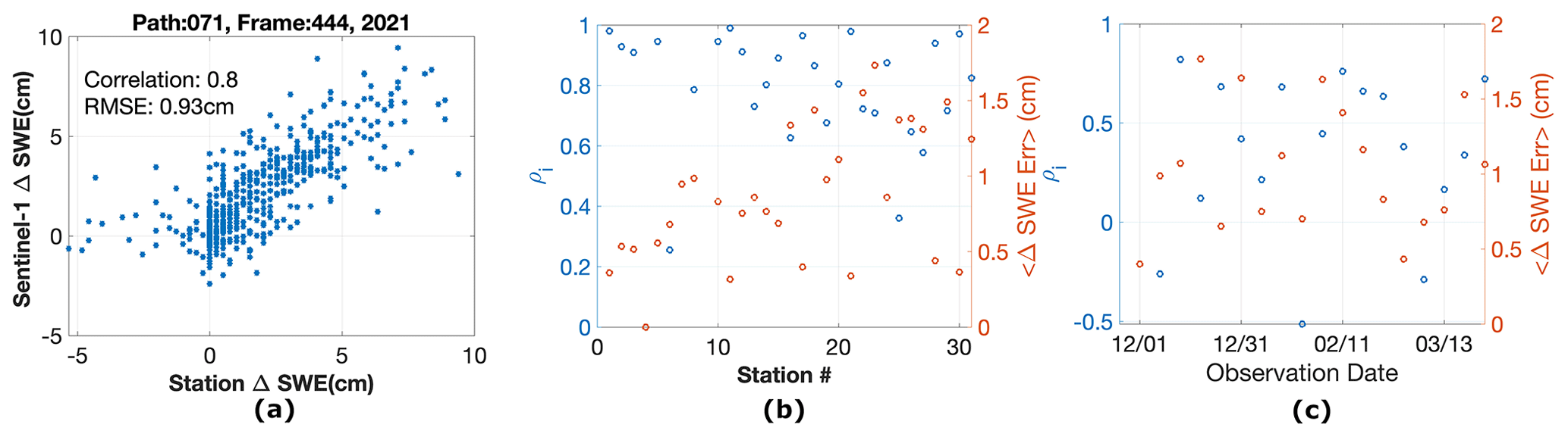
Figure 6(a) Retrieved ΔSWE using the Sentinel-1 interferometric phase versus in situ ΔSWE for all the stations with temporal coherence more than 0.35 for the entire Sentinel-1 time series from December 2020 to March 2021. (b) Correlation (left axis) and absolute error (right axis) between retrieved ΔSWE using the Sentinel-1 interferometric phase and in situ ΔSWE for each in situ station. (c) Correlation (left axis) and absolute error (right axis) between retrieved ΔSWE using the Sentinel-1 interferometric phase and in situ ΔSWE for each interferogram. Note that the labels on the x axis show the first date of each interferometric observation.
Figure 6a compares all the retrieved ΔSWE time series using Sentinel-1 data over all in situ stations with SNOTEL ΔSWE. As seen in this figure, the retrieved and in situ ΔSWE are highly correlated (0.8), with an RMSE of 0.93 cm.
Figure 6b shows the correlation and RMSE between the entire time series of retrieved and in situ ΔSWE for each station, with blue and red circles respectively. As seen in this figure, the correlation is good (more than 0.6 for all stations except three). The RMSE is less than 2 cm for all stations and less than 1 cm for most stations. Note that station 4 has just one observation with temporal coherence more than 0.35. That observation is the first observation with zero SWE change. Therefore, there are not enough points to calculate ρi. Hence, the RMSE and correlation are zero.
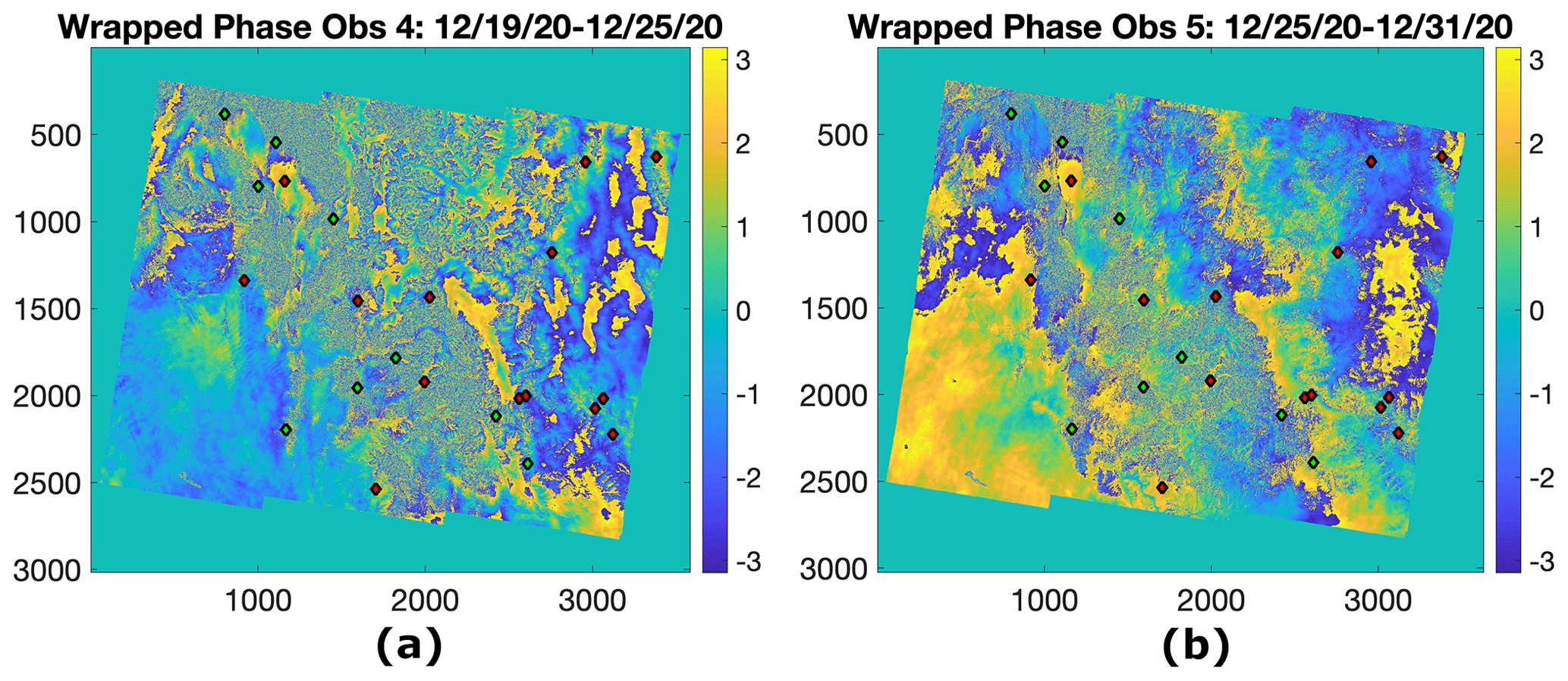
Figure 7Sentinel-1 wrapped phase path 71, frame 444, between (a) 19 and 25 December 2020 (observation 4) and (b) 25 and 31 December 2020 (observation 5).
Figure 6c shows the correlation and RMSE between the in situ stations and retrieved ΔSWE for each Sentinel-1 acquisition first date, with blue and red circles respectively. Note that the labels on the x axis show the first date of each interferometric observation. The RMSE is again less than 2 cm for all dates and less than 1 cm for many dates. As seen in this figure, the correlation is more than 0.4 for some dates and poor (less than 0.4) for some others. Among the observation dates with a correlation of less than 0.35 (observation 1, 2, 4, 7, 9, 15, 16, and 17), observations 1, 2, 7, 9, 15, and 16 (first date of 1 December, 7 December, 6 January, 18 January, 7 March, and 13 March) have very small snow accumulation (the average ΔSWE is less than 0.5 cm, with ΔSWE close to zero for most stations). Therefore, the phase is not sensitive enough to SWE change, hence the low correlation. For observation 4 and 17 (first date of 19 December and 19 March), we observed that the low coherence degrades the phase unwrapping performance for these InSAR images. Figure 7a and b show the wrapped phase for observations 4 and 5, respectively. Note that the correlation between in situ and retrieved ΔSWE in Fig. 6c is 0.1 for observation 4 and 0.7 for observation 5. The average in situ ΔSWE between 19 and 25 December 2020 (observation 4) is 1.6 cm and that between 25 and 31 December 2020 (observation 5) is 2.3 cm. However, the interferometric fringes in Fig. 7a are very noisy compared to Fig. 7b. We observe that 4 out of 6 d between 19 and 25 December 2020 (observation 4) are relatively warm, including day 19 December 2020. All 31 stations have temperatures between −7 and 6 ∘C at 06:00 in those 4 d. The warm days cause a lot of melting and refreezing in those 4 d. Hence, we expect to have small temporal coherence and consequently noisier fringes. On the other hand, the temperature is relatively warm only on 26 December 2020. The rest of the 5 d between 25 and 31 December 2020 (observation 5) are mostly colder than −7 ∘C for all 31 stations, thus resulting in higher temporal coherence and less noisier fringes. We believe the noisy fringes degrade the performance of the unwrapping algorithm significantly. Therefore, the retrieved ΔSWE is more accurate for observation 5 compared to observation 4. One of the main future works of this study is to improve the phase unwrapping over images with low coherence.
5.1.2 Comparing retrieved total SWE using Sentinel-1 and SNOTEL total SWE
In this section, we used time-series-retrieved ΔSWE to calculate total SWE at each date compared to the start date of our time series (1 December 2020) by
where t1 is 1 December 2020. For instance, SWE at 25 December 2020 compared to 1 December 2020 is the summation of all four retrieved ΔSWE (). Note that the SWE(ti+1) is measured compared to SWE(t1). For simplicity, we assume the SWE at time t1 is equal to zero.
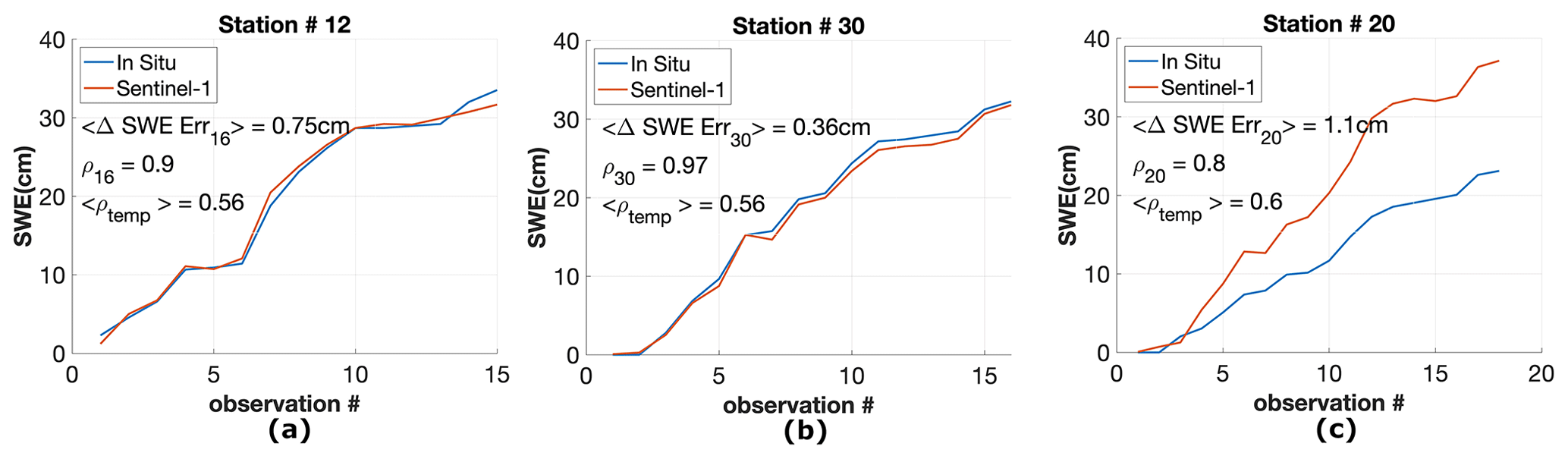
Figure 8Time series of total in situ and retrieved SWE using the Sentinel-1 interferometric phase shown by blue and red lines, respectively, for stations 12 (shown in panel a), 30 (b), and 20 (c).
Figure 8a, b, and c show the time series of total SWE for in situ stations 12, 30, and 20, respectively. Note that we used the average of stations 1 and 11 ΔSWE as a reference point in this study. The red and blue lines show the retrieved and in situ total SWE at each Sentinel-1 date acquisition compared to 1 December 2020. However, as mentioned in Sects. 4 and 5.1.1, we only used ΔSWE values with temporal coherence more than 0.35 and temperature less than 0 ∘C. We had 18 observations for the entire time series. Discarding some observation due to low temporal coherence or high temperature changes the time series length. As seen in Fig. 8, we keep all 18 observations for station 20 but only 15 observations for station 12.
As seen in this figure, the time series of total retrieved SWE aligns closely with in situ values for stations 12 and 30. The error is less than 2 cm in the entire time series. However, the retrieved SWE for station 20 diverges from in situ values even though it follows the same pattern. The error in total SWE estimation is about 10 cm at the end of the time series. We think the main reason for divergence is the phase unwrapping error and phase ambiguity. As discussed in Sect. 5.1.1, the noisy fringes degrade the performance of the unwrapping algorithm. A similar problem is observed in tower-based studies. The retrieval diverges from the in situ values by phase ambiguity values over large snowstorms at C-band (Fig. 13c in Ruiz et al., 2022). However, even in these cases, the trends of SWE remain the same between retrieved and in situ values. We will investigate the reason behind the divergence of retrieved SWE from in situ SWE of these stations in the future work of this study.
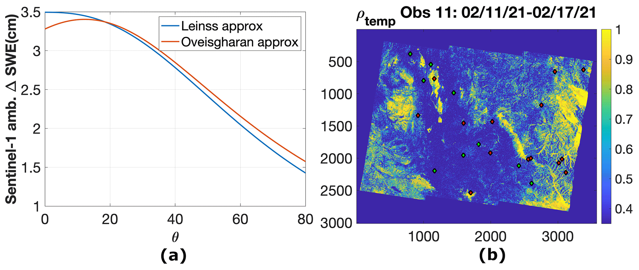
Figure 9(a) ΔSWE ambiguity versus incidence angle using Leinss's approximation (blue line) and Oveisgharan's approximation (red line) and (b) coherence for data acquired between 11 and 17 February 2021 (observation 11). Green diamonds show the location of stations with a total SWE error of less than 2 cm. Red diamonds show the location of stations with a total SWE error of more than 2 cm.
Figure 9a shows the Sentinel-1 ΔSWE ambiguity versus incidence angle. The red line shows the ΔSWE ambiguity using Eq. (4) (Δϕ=2π). The blue line shows the ΔSWE ambiguity using the Leinss et al. (2015) approximation (). As seen in this figure, ΔSWE ambiguity is between 1.5 and 3.5 cm depending on the incidence angle. The relatively small ΔSWE ambiguity of Sentinel-1 makes the unwrapping challenging for snowstorms. Figure 9b shows the temporal coherence between 11 and 17 February 2021. We can see very low coherence in the snowstorm regions, which degrades the unwrapping process. As mentioned before, one of the main future projects of this study is to work on improving the unwrapping phase.
For each station plot in Fig. 8, we also report the average RMSE error () and correlation (ρstation#) between retrieved and in situ ΔSWE, as also plotted in Fig. 6b. We also report the average of temporal coherence for all the interferograms over that station () to show how reliable the measurements at that station are. For all three stations, the RMSE error for ΔSWE is less than 1.1 cm, the correlation between in situ and retrieved ΔSWE is greater than 0.8, and temporal coherence is greater than 0.5. The SNOTEL sites are shown by small diamonds in Fig. 2b. The green small diamonds have a total SWE error of less than 2 cm in the entire time series, similar to stations 12 and 30. The red diamonds have a total SWE error of more than 2 cm, similar to station 20. However, the retrieved SWE has a similar pattern to in situ SWE. Therefore, we think they have a phase unwrapping problem similar to station 20. These stations are also shown in Fig. 7a. As seen in this figure, the red diamonds are mostly located in regions with noisy fringes, which makes the unwrapping challenging. Among all 31 stations in the Sentinel-1 frame, 6 of them have temporal coherence less than 0.35 or temperature more than 0 ∘C in their entire time series. These stations are shown by blue diamonds in Fig. 2b. Two stations are used for calibration of the phase. Hence, these two stations cannot be used for comparisons. So, there were 23 stations with more than two reliable observation dates in their time series. Among the 23 stations, 9 have an SWE error of less than 2 cm (green diamonds) and 14 of them have SWE error larger than 2 cm (red diamonds).
5.2 Comparing retrieved SWE using Sentinel-1 and lidar SWE
As mentioned in Sect. 3.3, the QSI lidar data were collected during the SnowEx campaign. There are two lidar data sets collected over the Sentinel-1 path 71, frame 444, in winter 2021. The locations are shown with red rectangles in Fig. 2b.
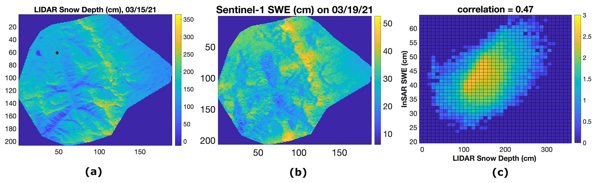
Figure 10(a) QSI lidar snow depth over Banner Summit, ID, on 15 March 2021 (b). Retrieved total SWE using Sentinel-1 interferometric data from 1 December 2020 to 19 March 2021 over Banner Summit, ID. (c) Two-dimensional histogram of data in panel (b) versus data in panel (a).
Figures 10a and 11a show the lidar snow depth on 15 March 2021 over Banner Summit and Mores Creek, respectively. As shown in Fig. 2b, Banner Summit covers SNOTEL 2 and Mores Creek covers SNOTEL 21. These two SNOTEL stations are shown by diamonds in Figs. 10a and 11a. The terrain DEM is measured by a lidar sensor during September 2021. The DEM is used to measure the snow depth using the lidar data collected on 15 March 2021. The big purple rectangle in Fig. 2b corresponds to Banner Summit, and the small red rectangle corresponds to Mores Creek. We calculated the total SWE compared to 1 December 2020 on the closest day to lidar date acquisition. We used all the retrieved ΔSWE from 1 December 2020 to 19 March 2021 and calculated the total SWE on 19 March 2021 using Eq. (5). Figures 10b and 11b show the retrieved SWE on 19 March 2021 over Banner Summit and Mores Creek, respectively. Panels (a) and (b) in Figs. 10 and 11 have very similar patterns. The 2D histograms of these two images are shown in Figs. 10c and 11c, where the x and y axes show the lidar snow depth and Sentinel-1-retrieved SWE, respectively. The colors in panel (c) show the 10number of cells with lidar snow depth x and InSAR SWE y. The correlation between these two data sets is 0.47 for Banner Summit and 0.59 for Mores Creek. Note that the lidar data show the snow depth, whereas Sentinel-1-retrieved data show the total SWE accumulated during the Sentinel-1 overpasses analyzed. On the other hand, lidar has a much higher resolution. The relatively good correlation (0.47 and 0.59) between the two independent measurements with different resolutions is a very good indication of the success of this method in estimating SWE.
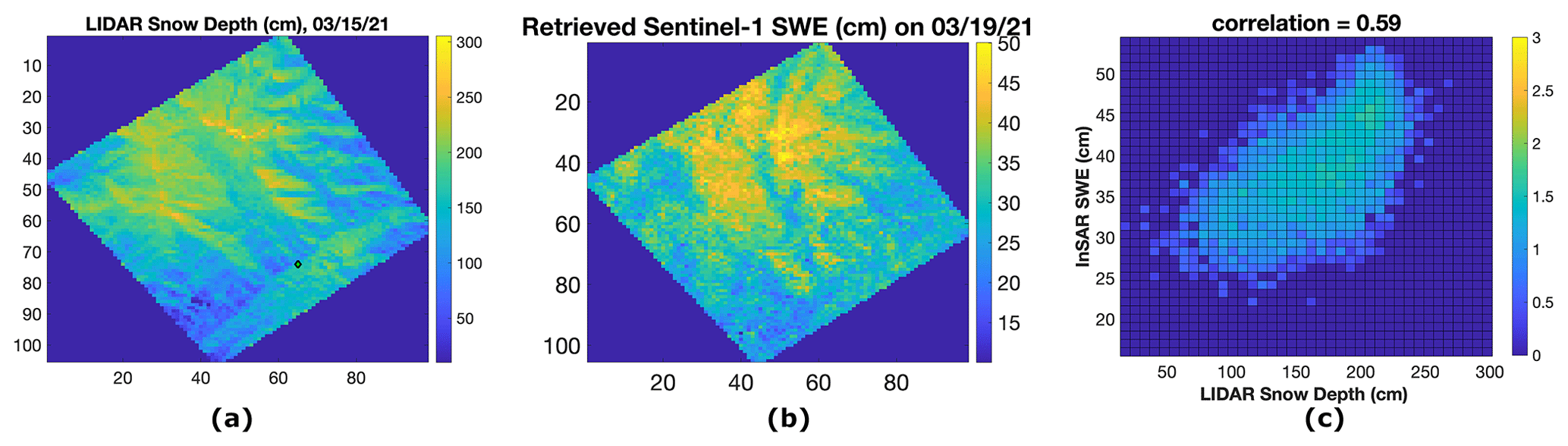
Figure 11(a) QSI lidar snow depth over Mores Creek, ID, on 15 March 2021. (b) Retrieved total SWE using Sentinel-1 interferometric data from 1 December 2020 to 19 March 2021 over Mores Creek, ID. (c) Two-dimensional histogram of data in panel (b) versus data in panel (a).
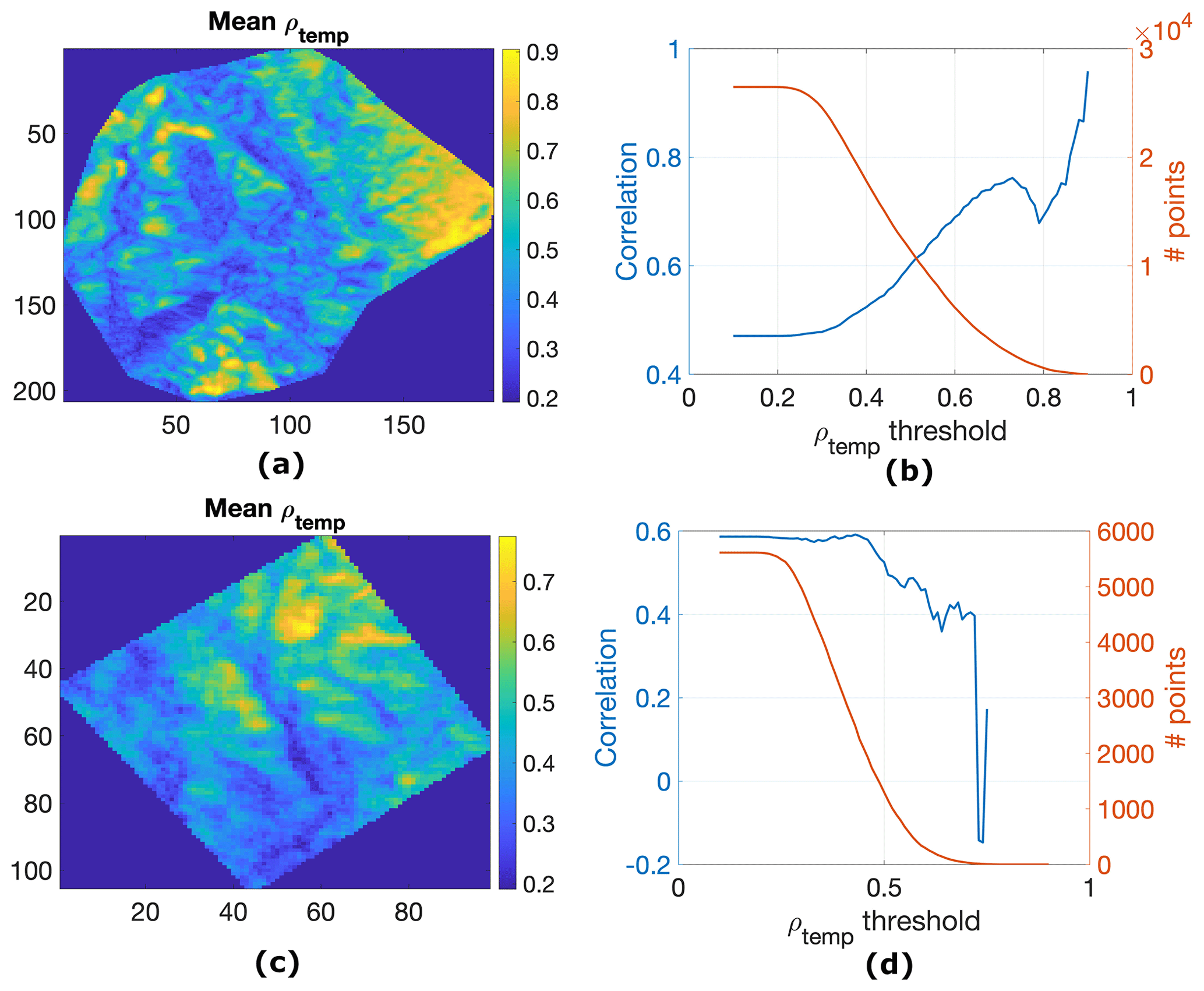
Figure 12(a) Mean of Sentinel-1 temporal coherence between 1 December 2020 and 19 March 2021 over Banner Summit, ID. (b) (Left axis) Correlation between lidar snow depth and retrieved total SWE on 19 March 2021 using Sentinel-1 over Banner Summit for all points with mean temporal coherence greater than ρtemp, threshold versus ρtemp, threshold. (Right axis) Number of points in Banner Summit with mean temporal coherence greater than ρtemp, threshold versus ρtemp, threshold. (c) Mean of Sentinel-1 temporal coherence between 1 December 2020 and 19 March 2021 over Mores Creek, ID. (d) (Left axis) Correlation between lidar snow depth and retrieved total SWE using Sentinel-1 over Mores Creek for all points with mean temporal coherence greater than ρtemp, threshold versus ρtemp, threshold. (Right axis) Number of points in Mores Creek with mean temporal coherence greater than ρtemp, threshold versus ρtemp, threshold.
Figure 12a and c show the mean of all Sentinel-1 temporal coherence data between 1 December 2020 and 19 March 2021 over Banner Summit and Mores Creek, respectively. As seen in these figures, the temporal coherence varies between 0.2 and 0.9. As mentioned earlier in this section, the correlation between lidar snow depth data on 15 March 2021 and retrieved total SWE using Sentinel-1 data on 19 March 2021 is 0.47 for Banner Summit and 0.59 for Mores Creek. However, some of the points may have low temporal coherence and may not be viable for retrieval as discussed in Sect. 4. The left axis in Fig. 12b and d show the correlation between lidar snow depth data on 15 March 2021 and retrieved total SWE using Sentinel-1 data on 19 March 2021 for points with mean temporal coherence above ρtemp, threshold. Figure 12b shows the correlation versus ρtemp, threshold over Banner Summit, and Fig. 12d shows the correlation over Mores Creek. Note that the correlation is 0.47 for Banner Summit and 0.59 for Mores Creek with no filter (ρtemp, threshold=0.1) as reported in Figs. 10c and 11c, respectively. The right axis in Fig. 12b and d shows the number of points in the image in panels (a) and (c) with mean temporal coherence more than ρtemp, threshold. There are 5 times more points in Fig. 12a compared to Fig. 12c. Therefore, we can better perform a statistical evaluation for panel (b) compared to panel (d). As seen in Fig. 12b, the correlation between lidar snow depth and retrieved total SWE increases by filtering out points with low temporal coherence, as expected. We need to investigate more to explain the reason for correlation decrease in the interval.
The correlation between lidar snow depth and retrieved total SWE in Fig. 12d) is relatively constant with increasing ρtemp, threshold. However, as we increase ρtemp, threshold to more than 0.46, the correlation gradually decreases to 0.4 at ρtemp, threshold=0.65 and remains relatively constant up to ρtemp, threshold=0.72. The number of points in the image with temporal coherence more than 0.72 is less than 20. Therefore, the correlation is not statistically very meaningful. Mores Creek has a lower elevation (6100 m at station 21) compared to Banner Summit (7040 m at station 2). Mores Creek is also warmer (mean temperature of −4.3 ∘C for the entire time series at station 21) than Banner Summit (mean temperature of −8.8 ∘C for the entire time series at station 3). We expect to have higher correlation with filtering low temporal coherence points as seen in Fig. 12b. We think the reason we do not see such a behavior in Fig. 12d is that the warmer temperature, melting, and refreezing degrade the retrieval performance even for highly correlated regions. More investigation is needed to better explain the constant or decreasing correlation with increasing ρtemp, threshold in Fig. 12d.
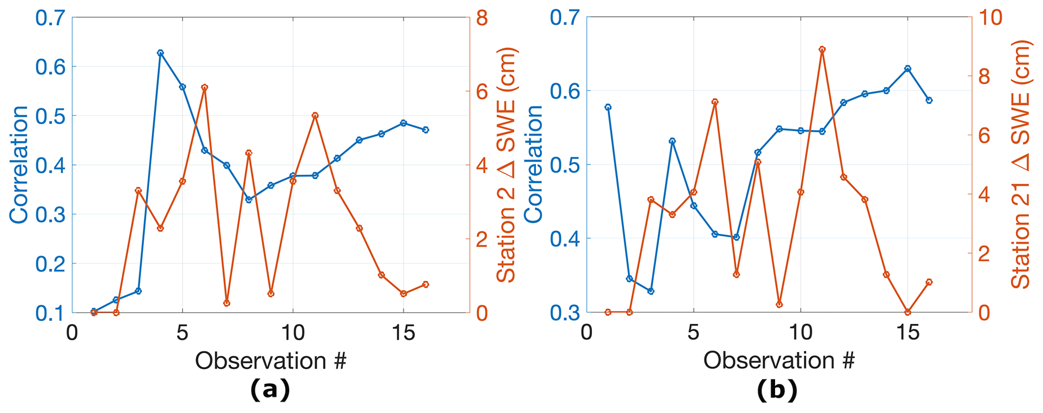
Figure 13(a) (Left axis) Correlation between lidar snow depth and retrieved total SWE using Sentinel-1 on a specific observation date over Banner Summit versus observation number. (Right axis) ΔSWE (cm) for any specific observation date at station 2 in Banner Summit. (b) (Left axis) Correlation between lidar snow depth and retrieved total SWE using Sentinel-1 on a specific observation date over Mores Creek versus observation number. (Right axis) ΔSWE (cm) for any specific observation date at station 27 in Mores Creek.
Left axis in Fig. 13a and b shows the correlation between lidar snow depth on 15 March 2021 and retrieved total SWE for each observation between 1 December 2020 and 19 March 2021 over Banner Summit and Mores Creek, respectively. Observation 16 shows the correlation reported in Figs. 10c and 11c. The right axis in Fig. 13a and b shows ΔSWE (cm) for each observation between 1 December 2020 and 19 March 2021 at station 2 in Banner Summit and station 21 in Mores Creek, respectively. As seen in both figures, the correlation gradually increases after observation 7 or 8, as expected. On the other hand, the correlation is smaller for observation 16 compared to 15. Observation 16 shows the total SWE on 19 March 2021, and lidar data show the snow depth on 15 March 2021. There is about 1 cm ΔSWE for observation 16 that is not fully captured by lidar. Therefore, comparing total SWE for observation 15 with lidar snow depth is more appropriate. The correlation is high for observation 4 at the beginning of the snow season for both Banner Summit and Mores Creek. Observation 4 is after the first snowstorm of the season. It shows that the spatial variability of snow at the end of the snow season is captured by the first or second snowstorm. Although ΔSWE for station 21 is zero for the first observation, the correlation between lidar snow depth on 19 March 2021 and total SWE on the first observation is relatively high, as seen in Fig. 13b. As shown in Fig. 11a, station 2 is in the relatively low snow depth region. We believe there has been a snowstorm in the high-altitude region of Mores Creek. The high correlation is simply the correlation between lidar data on 19 March 2021 and the first snowstorm in Mores Creek.
In this study, we used Sentinel-1 time series to retrieve ΔSWE and consequently total SWE. We chose a frame in Idaho that covers several SnowEx 2020–2021 sites and 31 SNOTEL in situ stations. Lidar data are available for validating our results. Sentinel-1 data were collected every 6 d over this SnowEx site instead of the regular 12 d, which helps a lot with temporal coherence over snowstorms. This provides a unique dense time series of spaceborne data for studying the performance of SWE retrieval using InSAR.
We showed that retrieved ΔSWE between two consecutive Sentinel-1 observations is highly correlated (0.8) with in situ values, with an RMSE of 0.93 cm. For the reference point of the interferometric phase, we used two in situ stations with temporal coherence more than 0.35 and temperature less than 0 ∘C for the entire time series. We subtracted the difference between the average of in situ and retrieved ΔSWE of these two stations from retrieved values to calibrate the retrieved ΔSWE. The ΔSWE RMSE error is less than 2 cm for all stations and less than 1 cm for most stations. The correlation between retrieved and in situ ΔSWE is more than 0.6 for most stations. Interferograms with a small average of in situ ΔSWE show low correlation between retrieved and in situ ΔSWE. We demonstrated that low temporal coherence not only degrades the SWE retrieval performance, but also the unwrapping algorithm performance. We showed that big melting events between two Sentinel-1 acquisitions make the interferometric fringes noisy and the unwrapping algorithm challenging. The retrieved total SWE has an RMSE error of less than 2 cm compared with in situ values in the entire time series for 9 stations and an error of more than 2 cm for 14 stations.
The highlight of the results of this study is the similarity between two independent measurements retrieved SWE using Sentinel-1 data and lidar snow depth data. We used Sentinel-1 data between 1 December 2020 and 19 March 2021 to retrieve ΔSWE time series. By adding the entire time series of ΔSWE, we calculated the total SWE on 19 March 2021. Total retrieved SWE values using Sentinel-1 interferometric data and lidar snow depth images over two regions in Idaho show similar patterns and are correlated by more than 0.47. We showed that the correlation is higher for regions with higher temporal coherence in Banner Summit.
Considering all these validations, we show for the first time that SWE retrieval using time series of InSAR spaceborne data is a very promising candidate for the future SWE mission.
We also show that the main constraints for this method are temporal coherence, phase unwrapping, and phase ambiguity. We show that snowstorms reduce the temporal coherence significantly. Low temporal coherence reduces the accuracy of the interferometric phase and unwrapping algorithm. This study all shows that melting due to warm temperature reduces the temporal coherence and the performance of the unwrapping algorithm. Small SWE ambiguity at C-band (1.5 to 3.5 cm) makes the phase unwrapping more challenging. We think using an in situ station as the reference point helps reduce the phase ambiguity error, at least locally, compared to other methods for referencing the interferometric images. If the temporal coherence is large enough for the entire image to reduce the phase unwrapping error, using the in situ SWE as the reference point reduces the phase ambiguity error in a larger region. Using a snow-free point or snow-free corner reflector as the reference point cannot address the phase ambiguity in regions with deep snow. Going from C-band to lower frequencies such as L-band improves both the temporal coherence and SWE ambiguity. With the L-band NISAR launch coming next winter, the new data set would be a great opportunity for global SWE retrieval.
The Sentinel-1 data are publicly available through the Alaska SAR Facility (ASF) or the Copernicus Data Hub distribution service. The SNOTEL data are free and available at the United States Department of Agriculture (USDA) website (https://wcc.sc.egov.usda.gov/nwcc/inventory, USDA, 2023). Finally, we collect the lidar data from the National Snow and Ice Data Center (https://doi.org/10.5067/VBUN16K365DG, Adebisi et al., 2022).
SO conceptualized the overall study. SO processed the data using HyP3. RZ applied atmospheric correction to the data. SO analyzed the data. ZH and HPM provided fruitful discussions and feedback and lidar data.
The contact author has declared that none of the authors has any competing interests.
Publisher's note: Copernicus Publications remains neutral with regard to jurisdictional claims made in the text, published maps, institutional affiliations, or any other geographical representation in this paper. While Copernicus Publications makes every effort to include appropriate place names, the final responsibility lies with the authors.
The research was carried out at the Jet Propulsion Laboratory, California Institute of Technology, under a contract with the National Aeronautics and Space Administration (grant no. 80NM0018D0004). The authors would like to thank Silvan Leinss and Jorge Jorge Ruiz for their very useful reviews that improved Sects. 2.2, 4, and 5.2 significantly.
This research has been supported by the Jet Propulsion Laboratory (R&TD 2022/2023).
This paper was edited by Nora Helbig and reviewed by Silvan Leinss and Jorge Jorge Ruiz.
Adebisi, N., Marshall, H., Vuyovich, C. M., Elder, K., Hiemstra, C., and Durand, M.: SnowEx20-21 QSI Lidar Snow Depth 0.5m UTM Grid, Version 1, Boulder, Colorado USA, NASA National Snow and Ice Data Center Distributed Active Archive Center [data set], https://doi.org/10.5067/VBUN16K365DG, 2022. a
Baduge, A. W. A., Henschel, M. D., Hobbs, S., Buehler, S. A., Ekman, J., and Lehrbass, B.: Seasonal variation of coherence in SAR interferograms in Kiruna, Northern Sweden, Int. J. Remote Sens., 37, 370–387, 2016. a
Barnett, T., Adam, J., and Lettenmaier, D.: Potential impacts of a warming climate on water availability in snow-dominated regions, Nature, 438, 303–309, 2005. a
Conde, V., Nico, G., Mateus, P., Catalão, J., Kontu, A., and Gritsevich4, M.: On the estimation of temporal changes of snow water equivalent by spaceborne SAR interferometry: a new application for the Sentinel-1 mission, J. Hydrol. Hydromech., 67, 93–100, 2019. a, b, c, d, e
Cui, Y., Xiong, C., Lemmetyinen, J., Shi, J., Jiang, L., Peng, B., Li, H., Zhao, T., Ji, D., and Hu, T.: Estimating Snow Water Equivalent with Backscattering at X and Ku Band on Absorption Loss, Remote Sens., 8, 505, https://doi.org/10.3390/rs8060505, 2016. a, b, c, d
Dagurova, P., Chimitdorzhieva, T., Dmitriev, A., and Dobryninb, S.: Estimation of snow water equivalent from L-band radar interferometry: simulation and experiment, Int. J. Remote Sens., 41, 9328–9359, https://doi.org/10.1080/01431161.2020.1798551, 2020. a, b, c, d, e
Deeb, E. J., Forster, R. R., and Kane, D. L.: Monitoring snowpack evolution using interferometric synthetic aperture radar on the North Slope of Alaska, Int. J. Remote Sens., 32, 3985–4003, 2011. a, b
Durand, M. and Liu, D.: The need for prior information in characterizing snow water equivalent from microwave brightness temperatures, Remote Sens. Environ., 126, 248–257, 2012. a
Eppler, J., Rabus, B., and Morse, P.: Snow water equivalent change mapping from slope-correlated synthetic aperture radar interferometry (InSAR) phase variations, The Cryosphere, 16, 1497–1521, https://doi.org/10.5194/tc-16-1497-2022, 2022. a, b, c, d
Gabriel, A. K., Goldstein, R. M., and Zebker, H. A.: Mapping small elevation changes over large areas: Differential radar interferometry, J. Geophys. Res., 94, 9183–9191, 1989. a
Gu, L., Fan, X., Li, X., and Wei, Y.: Snow Depth Retrieval in Farmland Based on a Statistical Lookup Table from Passive Microwave Data in Northeast China, Remote Sens., 11, 3037, https://doi.org/10.3390/rs11243037, 2019. a
Guneriussen, T., Hogda, K. A., Johnsen, H., and Lauknes, I.: InSAR for estimation of changes in snow water equivalent of dry snow, IEEE T. Geosci. Remote, 39, 2101–2108, 2001. a, b
Hogenson, K., Kristenson, H., Kennedy, J., Johnston, A., Rine, J., Logan, T., Zhu, J., Williams, F., Herrmann, J., Smale, J., and Meyer, F.: Hybrid Pluggable Processing Pipeline (HyP3): A cloud-native infrastructure for generic processing of SAR data, Zenodo [computer software], https://doi.org/10.5281/zenodo.4646138, 2020. a
Hoppinen, Z., Oveisgharan, S., Marshall, H.-P., Mower, R., Elder, K., and Vuyovich, C.: Snow water equivalent retrieval over Idaho – Part 2: Using L-band UAVSAR repeat-pass interferometry, The Cryosphere, 18, 575–592, https://doi.org/10.5194/tc-18-575-2024, 2024. a
H. Rott, T. N. and Scheiber, R.: Proceedings of the FRINGE 2003 Workshop (ESA SP-550), 1–5 December 2003, ESA/ESRIN, Frascati, Italy, edited by: Lacoste, H., Published on CDROM., id. 29, 2003. a
Hui, L., Pengfeng, X., Xuezhi, F., Guangjun, H., and Zuo, W.: Monitoring Snow Depth And Its Change Using Repeat-Pass Interferometric SAR In Manas River Basin, IGARSS, 4936–4939, 2016. a, b
Jolivet, R., Grandin, R., Lasserre, C., Doin, M., and Peltzer, G.: Systematic InSAR tropospheric phase delay corrections from global meteorological reanalysis data, Geophys. Res. Lett., 38, https://doi.org/10.1029/2011GL048757, 2011. a
Kellndorfer, J., Cartus, O., Lavalle, M., Magnard, C., Milillo, P., Oveisgharan, S., Osmanoglu, B., Rosen, P. A., and Wegmüller, U.: Global seasonal Sentinel-1 interferometric coherence and backscatter data set, Sci. Data, 9, 73, https://doi.org/10.1038/s41597-022-01189-6, 2022. a, b, c
Kelly, R.: The AMSR-E Snow depth algorithm: Description and initial results, J. Remote Sens. Soc. Jpn., 29, 307–317, 2009. a
Kelly, R. E., Chang, A. T., Tsang, L., and Foster, J. L.: A prototype AMSR-E global snow area and snow depth algorithm, IEEE T. Geosci. Remote, 41, 230–242, 2003. a, b
Lavalle, M., Simard, M., and Hensley, S.: A Temporal Decorrelation Model for Polarimetric Radar Interferometers, IEEE T. Geosci. Remote, 50, 2880–2888, https://doi.org/10.1109/TGRS.2011.2174367, 2012. a
Leinss, S., Parrella, G., and Hajnsek, I.: Snow Height Determination by Polarimetric Phase Differences in X-Band SAR Data, IEEE J. Sel. Top. Appl., 7, 3794–3810, 2014. a
Leinss, S., Wiesmann, A., Lemmetyinen, J., and Hajnsek, I.: Snow Water Equivalent of Dry Snow Measured by Differential Interferometry, IEEE J. Sel. Top. Appl., 8, 3773–3790, 2015. a, b, c, d, e, f, g, h, i, j, k, l, m, n, o
Lemmetyinen, J., Derksen, C., Rott, H., Macelloni, G., King, J., Schneebeli, M., Wiesmann, A., Leppanen, L., Kontu, A., and Pulliainen, J.: Retrieval of Effective Correlation Length and Snow Water Equivalent from Radar and Passive Microwave Measurements, Remote Sens., 10, 170, https://doi.org/10.3390/rs10020170, 2018. a, b, c, d
Lievens, H., Demuzere, M., Marshall, H.-P., Reichle, R. H., Brucker, L., Brangers, I., de Rosnay, P., Dumont, M., Girotto, M., Immerzeel, W. W., Jonas, T., Kim, E. J., Koch, I., Marty, C., Saloranta, T., Schöber, J., and Lannoy, G. J. D.: Snow depth variability in the Northern Hemisphere mountains observed from space, Nat. Commun., 10, 4629, https://doi.org/10.1038/s41467-019-12566-y, 2019. a, b, c
Lievens, H., Brangers, I., Marshall, H.-P., Jonas, T., Olefs, M., and De Lannoy, G.: Sentinel-1 snow depth retrieval at sub-kilometer resolution over the European Alps, The Cryosphere, 16, 159–177, https://doi.org/10.5194/tc-16-159-2022, 2022. a
Liu, Y., Li, L., Yang, J., Chen, X., and Hao, J.: Estimating Snow Depth Using Multi-Source Data Fusion Based on the D-InSAR Method and 3DVAR Fusion Algorithm, Remote Sens., 9, 1195, https://doi.org/10.3390/rs9111195, 2017. a, b, c
Luzi, G., Noferini, L., Mecatti, D., Macaluso, G., Pieraccini, M., Atzeni, C., Schaffhauser, A., Fromm, R., and Nagler, T.: Using a ground-based SAR interferometer and a terrestrial laser scanner to monitor a snow-covered slope: Results from an experimental data collection in Tyrol, IEEE T. Geosci. Remote, 47, 382–393, 2009. a
Marshall, H., Deeb, E., Forster, R., Vuyovich, C., Elder, K., Hiemstra, C., and Lund, J.: L-Band InSAR Depth Retrieval During the NASA SnowEx 2020 Campaign: Grand Mesa, Colorado, 2021 IEEE International Geoscience and Remote Sensing Symposium IGARSS, Brussels, Belgium, 2021, 625–627, https://doi.org/10.1109/IGARSS47720.2021.9553852, 2021. a, b, c
Marshall, H.-P. and Koh, G.: FMCW radars for snow research, Cold Reg. Sci. Technol., 52, 118–131, 2008. a
Mätzler, C.: Application of the interaction of Microwave with the Natural Snow Cover, Remote Sensing Reviews, 2, 259–387, 1987. a
Molan, Y. E., Kim, J.-W., Lu, Z., and Agram, P.: L-band temporal coherence assessment and modeling using amplitude and snow depth over interior Alaska, Remote Sens., 10, 1216–1228, 2018. a
Nagler, T., Rott, H., Scheiblauer, S., Libert, L., Mölg, N., Horn, R., Fischer, J., Keller, M., Moreira, A., and Kubanek, J.: Airborne experiment on insar snow mass retrieval in alpine environment, IGARSS, 4549–4552, https://doi.org/10.1109/IGARSS46834.2022.9883809, 2022. a, b, c, d, e, f
Nghiem, S. V. and Tsai, W. Y.: Global snow cover monitoring with spaceborne Ku:band scatterometer, IEEE T. Geosci. Remote, 39, 2118–2134, 2001. a
Oveisgharan, S. and Zebker, H.: Estimating Snow Accumulation From InSAR Correlation Observations, IEEE T. Geosci. Remote, 45, 10–20, 2007. a
Oveisgharan, S., Esteban-Fernandez, D., Waliser, D., Friedl, R., Nghiem, S., and Zeng, X.: Evaluating the Preconditions of Two Remote Sensing SWE Retrieval Algorithms over the US, Remote Sens., 12, 2021, https://doi.org/10.3390/rs12122021, 2020. a
Painter, T. H., Berisford, D. F., Boardman, J. W., Bormann, K. J., Deems, J. S., Gehrke, F., Hedrick, A., Joyce, M., Laidlaw, R., Marks, D., Mattmann, C., McGurk, B., Ramirez, P., Richardson, M., McKenzie Skiles, S., Seidel, F. C., and Winstral, A.: The Airborne Snow Observatory: Fusion of scanning LiDAR, imaging spectrometer, and physically-based modeling for mapping snow water equivalent and snow albedo, Remote Sens. Environ., 184, 139–152, 2016. a
Pulliainen, J. and Hallikainen, M.: Retrieval of regional snow water equivalent from space-borne passive microwave observations, Remote Sens. Environ., 75, 76–85, 2001. a
Rott, H., Yueh, S. H., Cline, D. W., Duguay, C., Essery, R., Haas, C., Heliere, F., Kern, M., Macelloni, G., and Malnes, E.: Cold regions hydrology high-resolution observatory for snow and cold land processes, Proc. IEEE 2010, 98, 752–765, 2010. a, b
Ruiz, J. J., Lemmetyinen, J., Kontu, A., Tarvainen, R., Vehmas, R., Pulliainen, J., and Praks, J.: Investigation of Environmental Effects on Coherence Loss in SAR Interferometry for Snow Water Equivalent Retrieval, IEEE T. Geosci. Remote Sens., 60, 4306715, https://doi.org/10.1109/TGRS.2022.3223760, 2022. a, b, c, d, e, f, g, h
Shah, R., Xu, X., Yueh, S., Chae, C. S., Elder, K., Starr, B., and Kim, Y.: Remote Sensing of Snow Water Equivalent Using P-Band Coherent Reflection, Geosci. Remote Sens. Lett., 14, 309–313, 2017. a, b
Takala, M., Luojus, K., Pulliainen, J., Derksen, C., and and, J. L.: Estimating northern hemisphere snow water equivalent for climate research through assimilation of space-borne radiometer data and ground-based measurements, Remote Sens. Environ., 115, 3517–3529, 2011. a, b
Tao, M., Su, J., Huang, Y., and Wang, L.: Mitigation of Radio Frequency Interference in Synthetic Aperture Radar Data: Current Status and Future Trends, Remote Sens., 11, 2438, https://doi.org/10.3390/rs11202438, 2019. a
Tarricone, J., Webb, R. W., Marshall, H.-P., Nolin, A. W., and Meyer, F. J.: Estimating snow accumulation and ablation with L-band interferometric synthetic aperture radar (InSAR), The Cryosphere, 17, 1997–2019, https://doi.org/10.5194/tc-17-1997-2023, 2023. a
Ulaby, F. T. and Stiles, W. H.: The active and passive microwave response to snow parameters: 2. Water equivalent of dry snow., J. Geophys. Res.-Oceans, 85, 1045–1049, 1980. a
USDA: Public Reports | Air & Water Database Public Reports, USDA [data set], https://wcc.sc.egov.usda.gov/nwcc/inventory, last access: August 2023. a
Yueh, S. H., Xu, X., Shah, R., Kim, Y., Garrison, J. L., Komanduru, A., and Elder, K.: Remote Sensing of Snow Water Equivalent Using Coherent Reflection From Satellite Signals of Opportunity: Theoretical Modeling, IEEE J. Sel. Top. Appl., 10, 5529–5540, 2017. a, b, c
Yueh, S. H., Shah, R., Xu, X., Stiles, B., and Bosch-Lluis, X.: A Satellite Synthetic Aperture Radar Concept Using P-Band Signals of Opportunity, IEEE J. Sel. Top. Appl., 14, 2796–2816, 2021. a, b
Yunjun, Z., Fattahi, H., and Amelung, F.: Small baseline InSAR time series analysis: Unwrapping error correction and noise reduction, Comput. Geosci., 133, 5529–5540, 2019. a
Zebker, H. A. and Villasenor, J.: Decorrelation in Interferometric Radar Echoes, IEEE T. Geosci. Remote, 30, 950–959, 1992. a
Zebker, H. A., Rosen, P. A., Goldstein, R., Gabriel, A., and L.Werner, C.: On the derivation of coseismic displacement fields using differential radar interferometry: The Landers earthquake, J. Geophys. Res.-Sol. Ea., 99, 19617–19634, 1994. a
- Abstract
- Copyright statement
- Introduction
- Using differential interferometry to estimate SWE
- Data sets
- SWE retrieval using the Sentinel-1 interferometric phase
- Results and discussions
- Conclusions
- Data availability
- Author contributions
- Competing interests
- Disclaimer
- Acknowledgements
- Financial support
- Review statement
- References