Passive microwave remote-sensing-based high-resolution snow depth mapping for Western Himalayan zones using multifactor modeling approach

Spatiotemporal snow depth (SD) mapping in the Indian Western Himalayan (WH) region is essential in many applications pertaining to hydrology, natural disaster management, climate, etc. In situ techniques for SD measurement are not sufficient to represent the high spatiotemporal variability in SD in the WH region. Currently, low-frequency passive microwave (PMW) remote-sensing-based algorithms are extensively used to monitor SD at regional and global scales.

However, fewer PMW SD estimation studies have been carried out for the WH region to date, which are mainly confined to small subregions of the WH region. In addition, the majority of the available PMW SD models for WH locations are developed using limited data and fewer parameters and therefore cannot be implemented for the entire region. Further, these models have not taken the auxiliary parameters such as location, topography, and snow cover duration (SCD) into consideration and have poor accuracy (particularly in deep snow) and coarse spatial resolution.

Considering the high spatiotemporal variability in snow depth characteristics across the WH region, region-wise multifactor models are developed for the first time to estimate SD at a high spatial resolution of 500 m × 500 m for three different WH zones, i.e., Lower Himalayan Zone (LHZ), Middle Himalayan Zone (MHZ), and Upper Himalayan Zone (UHZ). Multifrequency brightness temperature (TB) observations from Advanced Microwave Scanning Radiometer 2 (AMSR2), SCD data, terrain parameters (i.e., elevation, slope, and ruggedness), and geolocation for the winter period (October to March) during 2012–2013 to 2016–2017 are used for developing the SD models for dry snow conditions. Different regression approaches (i.e., linear, logarithmic, reciprocal, and power) are used to develop snow depth models, which are evaluated further to find if any of these models can address the heterogeneous association between SD observations and PMW TB. From the results, it is observed from the analysis that the power regression SD model has improved accuracy in all WH zones with the low root mean square error (RMSE) in the MHZ (i.e., 27.21 cm) compared to the LHZ (32.87 cm) and the UHZ (42.81 cm). The spatial distribution of model-derived SD is highly affected by SCD, terrain parameters, and geolocation parameters and has better SD estimates compared to regional and global products in all zones. Overall results indicate that the proposed multifactor SD models have achieved higher accuracy in deep snowpack (i.e., SD >25 cm) of the WH region compared to previously developed SD models.

1 Introduction

Snow is an essential land cover type and an important cryosphere component. The snow cover encompasses an aerial extent of approximately 45 × 10⁶ km² in the peak winter over the Northern Hemisphere (Estilow et al., 2015; Lemke et al., 2007). Among many cryosphere regions in the Northern Hemisphere, the Indian Western Himalayan (WH) region is a unique snow-covered region with a complex topography and high spatiotemporal variability in snow depth (SD) and diverse land cover types (Singh et al., 2018; Das and Sarwade, 2008; Thakur et al., 2019; Sharma et al., 2014; Singh et al., 2016). The WH region comprises three mountain zones, e.g., Lower Himalayan Zone (LHZ), Middle Himalayan Zone (MHZ), and Upper Himalayan Zone (UHZ), and receives significant snowfall during winter (Dimri and Dash, 2012; Gurung et al., 2011; Kumar et al., 2019; Sharma and Ganju, 2000; Singh et al., 2016, 2014). The variation in snow volume and its melt rate affects the availability of fresh water for drinking, hydropower, irrigation facilities, and ecosystem conditions for millions of people residing in the foothills of WH zones (Singh et al., 2016; Thakur et al., 2019; Nüsser et al., 2019; Negi et al., 2020; Ahmad, 2020; Mukherji et al., 2019; Vishwakarma et al., 2022). Further, the variability in snow characteristics such as SD, density, and volume and mountainous topography triggers frequent avalanches in the WH region, which have resulted in more than 1000 casualties as reported in different studies (Ganju et al., 2002; McClung, 2016; Gusain et al., 2016). Therefore, quantifying snow variables, especially SD, is an essential field of study in the WH region.

Traditionally SD information is acquired using in situ measurements from snow stakes, snow poles, ground penetrating radar, automatic weather stations, etc. (Dong, 2018; Kinar and Pomeroy, 2015). In situ methods provide accurate SD; however, these techniques have several drawbacks, such as limited spatial coverage, operational and maintenance constraints under harsh weather and complex terrain conditions, instrument calibration and malfunctioning issues, and high logistics and personnel requirements (Kinar and Pomeroy, 2015; Gusain et al., 2016). In the WH region, because of the rocky terrain and harsh climatic conditions, a sparse network of snow monitoring stations is available (Saraf et al., 1999; Singh et al., 2016; Gusain et al., 2016). Apart from this, the available SD observations from the in situ network are spatially and temporally discontinuous and inadequate for demonstrating the snowpack at a regional scale, particularly in the high-altitude regions of the WH region. Spaceborne passive microwave (PMW) remote sensing observations can partially compensate for these limitations and effectively monitor large areas for SD at a comparatively low cost under all weather and terrain conditions (Dietz et al., 2012; Amlien, 2008; Bernier, 1987; Xiao et al., 2018). Sensitivity to snowpack characteristics, global coverage, daily temporal resolution, and availability of an extensive archive of historical data make spaceborne PMW remote sensing data extensively useful for the retrieval of SD (Dietz et al., 2012; Tedesco and Narvekar, 2010; Luojus et al., 2021; Chang et al., 1987).

The historical PMW data and ongoing and planned missions have paved the way for developing numerous SD inversion algorithms across the different cryosphere regions of the earth. Many studies of SD estimation have been carried out using multifrequency brightness temperature (TB) observations collected from PMW sensors on board different satellites (Chang et al., 1987; Saraf et al., 1999; Xiao et al., 2018; Kelly et al., 2005; Takala et al., 2011; Dai et al., 2018; Jiang et al., 2014; Singh et al., 2012). The volumetric PMW scattering increases while PMW TB decreases with an increase in SD. The PMW brightness temperature difference (BTD) of 18 and 36 GHz frequency increases with an increase in SD up to a specific thickness and then saturates depending on snowpack conditions (Rango et al., 1979; Chang et al., 1987; Tedesco and Narvekar, 2010). Hence, many studies of PMW SD inversion relied on empirical models derived using BTD between 18 and 36 GHz frequency from TB observations (Chang et al., 1987; Saraf et al., 1999; Foster et al., 1997; Kelly et al., 2005, 2003; Das and Sarwade, 2008). Many of the empirical models for SD are developed by generalizing the snowpack parameters such as snow density and grain size (Chang et al., 1987, 1997; Kelly et al., 2003). However, these parameters dynamically vary with space and time. As a result, the applicability of many empirical SD models (Chang et al., 1987; Foster et al., 1997; Aschbacher, 1989) outside their study region is not good, as evident from several studies (Dai et al., 2018; Wang et al., 2019, 2020; Saraf et al., 1999; Xiao et al., 2018). Further, many PMW studies have shown that the error in estimated SD using TB data varies with snow conditions (i.e., wetness, grain size, density), land cover, topography, ground SD, etc. (Dai et al., 2018; Tedesco and Narvekar, 2010; Tedesco et al., 2010; Kelly et al., 2002; Yang et al., 2021; Wang et al., 2010; Ansari et al., 2019). Different combinations of multifrequency PMW TB observations, snow information (i.e., snow cover fraction, grain size, density), and auxiliary data such as topographical and land cover information are used in the PMW-based SD model development to account for these limitations (Dai et al., 2018; Wang et al., 2020, 2019). Many SD modeling approaches comprising static empirical linear (Chang et al., 1987; Saraf et al., 1999; Singh et al., 2012) and nonlinear models (Wang et al., 2020, 2019), dynamic models (Tedesco et al., 2010; Grippa et al., 2004; Wei et al., 2021), snow emission models (Dai et al., 2018; Yang et al., 2021), machine learning algorithms (Xiao et al., 2018; Yang et al., 2020), assimilation schemes (Kwon et al., 2017; Graf et al., 2006), etc., have been developed using PMW TB and auxiliary datasets for different regions.

Despite the significant progress in PMW-based SD estimation, very few studies have been carried out in the Indian WH region using PMW data (Singh et al., 2012; Das and Sarwade, 2008; Saraf et al., 1999; Singh et al., 2015). The WH region, being a tropical region, experiences significant changes in temperature, leading to frequent melt–freeze snow events causing snow grain growth, which introduces errors in the estimation of PMW SD (Singh et al., 2015). Further, the limited availability of in situ SD observations, very high SD (i.e., >1 m), and high spatiotemporal variability in snowpack characteristics pose numerous constraints for PMW SD estimation in the WH region. Consequently, no studies were reported for PMW SD estimation in WH till 1999. For the first time, Saraf et al. (1999) estimated the average monthly SD using Scanning Multichannel Microwave Radiometer (SMMR) data on board Nimbus-7 during 1979–1987 for the Sutlej valley region of Himalaya using the modified Chang model (Chang et al., 1992). However, the applicability of this model (Saraf et al., 1999; Chang et al., 1992) over the entire Himalaya cannot be justified as the model is developed using less in situ data (from 11 stations) where the stations are not distributed and is not tested outside the Sutlej basin. Singh and Mishra (2006) have proposed three empirical models using Advanced Scanning Microwave Radiometer for Earth (AMSR-E) data (horizontally polarized TB of 18.7 and 36.5 GHz) for SD estimation in the Pir Panjal, Greater Himalaya, and Karakoram ranges of the WH region. Following this study, Singh et al. (2007) used different empirical models for SD estimation using multifrequency Special Sensor Microwave/Imager (SSM/I) data (i.e., TB of 19, 22, 37, and 89 GHz during 1997–2002) over the Patseo region. However, these studies (Singh and Mishra, 2006; Singh et al., 2007; Saraf et al., 1999) have not provided any quantitative details about the accuracy of SD estimates and have not been evaluated using independent SD observations. Das and Sarwade (2008) used 18.7 and 36.5 GHz horizontally polarized data from AMSR-E and modified the coefficients of Chang et al.'s (1987) model to suit the Indian Himalaya. The modified model has shown a mean absolute error (MAE) of 20.34 cm in SD estimates but failed to estimate SD above 60 cm. Singh et al. (2012) have developed multiple empirical SD models for three SD classes, i.e., 1 to 5, 5 to 50, and 50 to 200 cm, in the Pir Panjal, Greater Himalayan, and Karakoram regions of the WH region using TB data of different frequencies from SSM/I. Their approach (Singh et al., 2012) has used the scattering index to estimate snow cover and TB thresholds for identifying the SD class and estimation of SD. In another study, Singh et al. (2015) developed PMW SD models for the Dhundi and Patseo regions of Himalaya using data from ground-based radiometers and in situ observations. However, SD models were developed using observations collected from only two field surveys, evaluated using a single-day observation of AMSR-E TB data, and not tested spatiotemporally. Recently, Singh et al. (2020) developed an empirical algorithm for the Patseo region of the MHZ using Advanced Microwave Scanning Radiometer 2 (AMSR2) 18.7 and 36.5 GHz TB (i.e., during 2012–2016) and in situ observations. They observed that the estimated SD is very close to ground data with a root mean square error (RMSE) of ∼ 16 cm and MAE of ∼ 13.9 cm.

Despite the development of various PMW SD models for Himalaya in the last 2 decades (1999–2020), there are many constraints in the spatiotemporal estimation of SD for the WH region. Many of the previous studies for SD estimation in the WH region have been carried out specifically for subregions of the WH region, such as the Sutlej basin, Dhundi, and Patseo. The PMW TB observations are affected by heterogeneity in snowpack properties, land cover, topography, etc. (Trujillo et al., 2007; Wang et al., 2010; Che et al., 2016; Derksen, 2008; Foster et al., 2005). However, previous studies (Das and Sarwade, 2008; Saraf et al., 1999; Singh et al., 2012, 2020, 2007; Singh and Mishra, 2006) have not accounted for the aforementioned variables. Further, the accuracy of SD retrievals from these models is also not evaluated with respect to the varying terrain and snow parameters. The accuracy of operational PMW SD products available in the WH region, i.e., AMSR2 SD, has not been evaluated.

Additionally, the AMSR2 SD product and previous PMW SD models have course resolution and have limitations on their potential utility in various applications such as avalanche susceptibility and hydrological modeling, especially at the regional scale. Considering these research gaps, in the current study, different linear and nonlinear empirical models are developed to improve and estimate SD at high resolution, i.e., 500 m for different WH zones, using a multifactor approach. In this approach, multifrequency PMW observations from AMSR2 (during 2012–2019), terrain parameters, land cover parameters, and the Moderate Resolution Imaging Spectroradiometer (MODIS)-derived snow cover product are statically correlated with the ground SD observations for the development and evaluation of the SD models. The accuracy of PMW multifactor SD models' estimates is compared with previous models and the AMSR2 SD product. Further, in this study, the SD retrieval accuracy is also analyzed with respect to different auxiliary parameters. The present study has the following three objectives:

• development of multifactor SD models to estimate SD at high resolution for different WH zones;

• comparison and evaluation of the proposed multifactor model, previous SD models, and AMSR2 SD products in different WH zones;

• analysis of multifactor SD retrieval accuracy with respect to selected auxiliary variables (i.e., elevation, slope, land cover types, and snow cover duration – SCD).

Following this introduction section (Sect. 1), the current article is organized as follows. The topographical and geographical description of the study area is described in Sect. 2. The details of the in situ observation network and various remote sensing datasets used for model development and evaluation are also given in the same section. Following that, the methodology used in developing the multifactor model is presented in Sect. 3. Subsequently, Sect. 4 describes the performance of different multifactor models developed for the three WH zones, a comparison of the different SD models, and results from the analysis of multifactor SD model retrievals with respect to auxiliary parameters. The discussion and summary are given in Sects. 5 and 6, respectively.

2 Study area and datasets

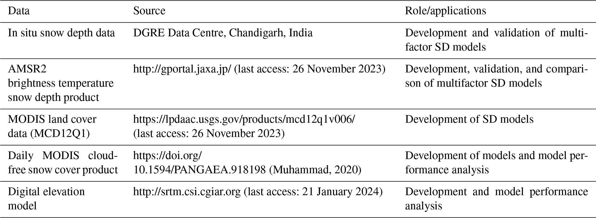
The topographic and environmental conditions prevailing in the WH region are detailed in Sect. 2.1. This study makes use of in situ data from the snow monitoring network and various spaceborne data for the development of SD models for different WH zones. These datasets along with their sources are listed in Table 1 and briefly discussed in the following subsections from 2.2 to 2.7.

Table 1 Sources of in situ, remote sensing datasets and their application in the present study.

2.1 Study area

Himalaya is the largest snow-covered territory outside the polar regions in the world (Gurung et al., 2011). The present study encompasses the entire WH region, which is a significant portion of the Indian Himalaya, situated in the states of Jammu and Kashmir, Ladakh, and Himachal Pradesh (see Fig. 1). The WH region extends between longitudes from 73^∘15^′ to 79^∘45^′ E and latitudes from 30^∘00^′ to 39^∘ N and covers an area of 360 866 km². The WH region is unique with its perennial snow-covered mountain peaks and seasonal snow-covered valleys. Approximately 65 % of the terrain in the WH region is situated at an altitude of more than 3000 m a.m.s.l. (above mean sea level) and is underlain by extremely steep and rugged mountains. The high-altitude terrain and mountain topography influence both winter precipitation (caused by western disturbances) and monsoon precipitation patterns (Dimri and Dash, 2012). Due to prevailing topographical and weather conditions in the WH region, forest cover is present only up to 3000 m a.m.s.l., and between 3000–4000 m a.m.s.l. thin vegetation consisting of shrubs and grass is present, whereas above 4000 m a.m.s.l. altitude, vegetation is not present, and the land cover there is predominantly comprised of barren land with snow and ice. The WH region generally receives snow from October to March; from April onwards, snowmelt generates runoff contributing water to many rivers and streams within the region (Dimri and Dash, 2012; Sharma et al., 2014).

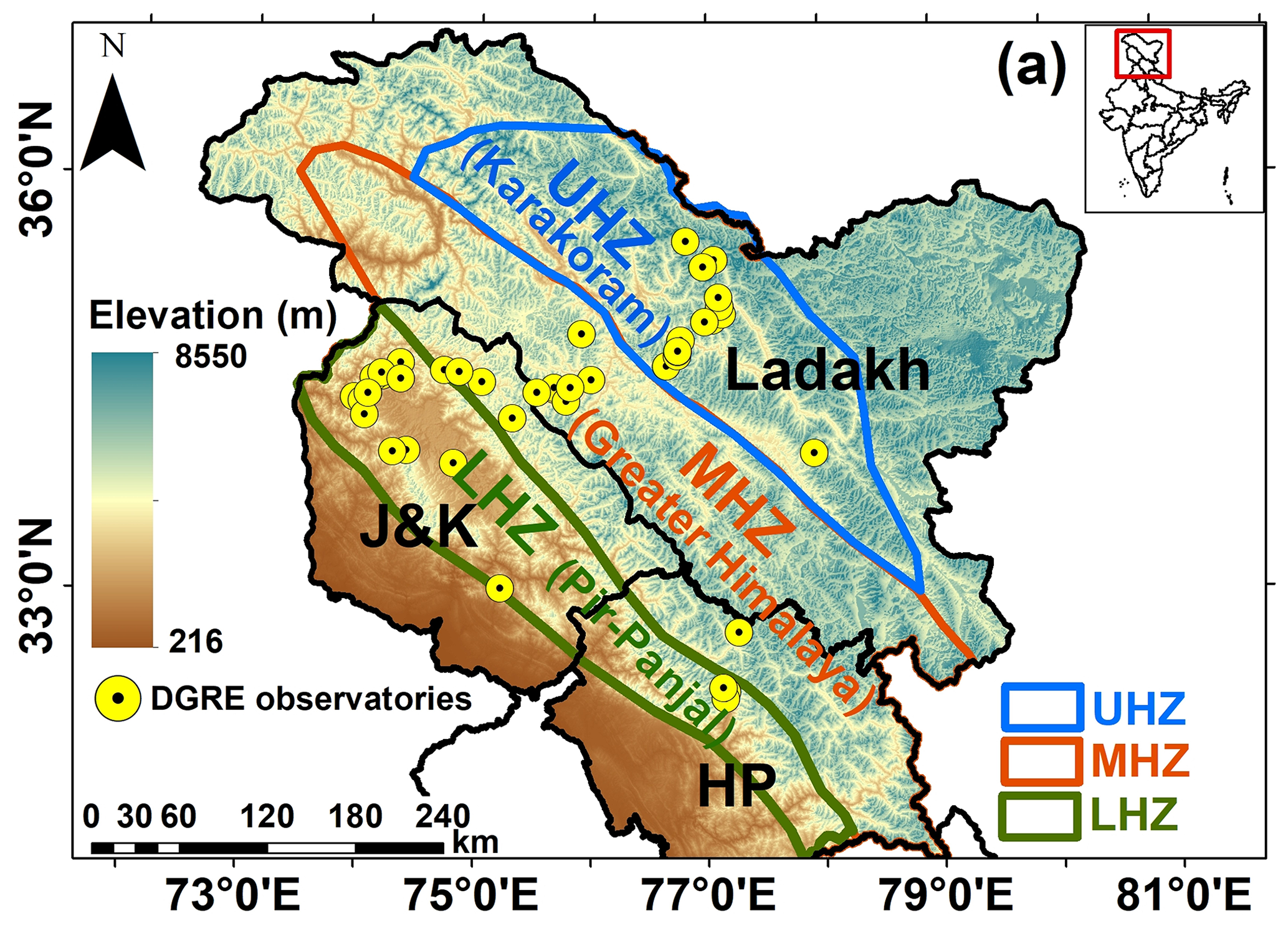
Figure 1 (a) Elevation variability in WH zones (i.e., LHZ: Lower Himalayan Zone; MHZ: Middle Himalayan Zone; UHZ: Upper Himalayan Zone) and DGRE observatory distribution (Note: J&K is Jammu and Kashmir, HP is Himachal Pradesh).

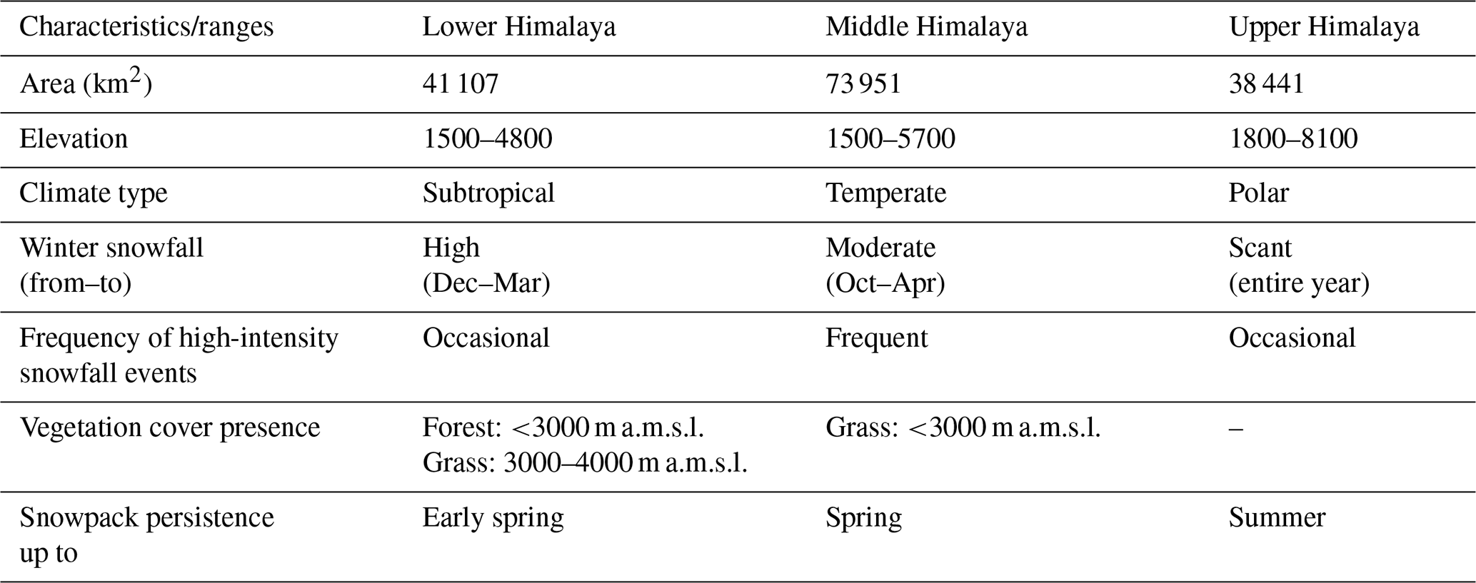
In this study, three WH zones, i.e., LHZ, MHZ, and UHZ, defined based on the historical local meteorological and avalanche occurrence data (Sharma and Ganju, 2000), are used for developing multifactor SD models. The geomorphic and climate characteristics of these zones are given in Table 2. The three zones differ in regional topographical and climatic conditions with varying elevations, temperatures, rainfall, snowfall, etc. The LHZ has a subtropical climate, and the MHZ has a temperate climate, while the UHZ has polar climatic conditions with the presence of permanent snow. Further, these zones have different timings and intensities of precipitation. The LHZ has comparatively warmer conditions, with mean monthly temperatures varying between (−3 to 18 ^∘C), than the MHZ (−10 to 14 ^∘C) and UHZ (−25 to 0 ^∘C). As the latitude increase, the amount of precipitation deceases in the WH region. Negi et al. (2018) reported average winter precipitation (in terms of snow water equivalent) of ∼ 804, 549, and 431 mm in the LHZ, MHZ, and UHZ, respectively, during 1991–2015. Further, the snowpack persistence varies based on the local weather conditions, which mainly changes with elevation across the three WH zones (Sharma et al., 2014).

Table 2 Geomorphic characteristics of the WH zones.

2.2 Ground observatory stations data

In the WH region, the Defence Geoinformatics Research Establishment (DGRE) (formally known as Snow and Avalanche Research Establishment) operates and maintains a network of 43 observatory stations (see Fig. 1) which measures daily in situ SD twice (i.e., forenoon and afternoon) along with other meteorological parameters such as temperature and rainfall. Out of total 43 stations, 16 stations are located in the LHZ, 13 in the MHZ, and 14 in the UHZ. From the LHZ, MHZ, and UHZ observatories, elevation varies between 1652 and 3785 m a.m.s.l., 2440 and 4950 m a.m.s.l., and 3960 and 5995 m a.m.s.l., respectively. In this study, in situ data comprising station name, date, latitude, longitude, and SD for the 43 stations are obtained for the snow period from 2012–2013 to 2018–2019. The in situ data are grouped according to the WH zones for the development of different multifactor SD models. The mean in situ SD of stations varies between 11 and 256 cm in the LHZ, 23 and 136 cm in the MHZ, and 52 and 356 cm in the UHZ during the study period.

2.3 AMSR2 brightness temperatures data

AMSR2 is a PMW sensor on board the Japanese Aerospace Exploration Agency's (JAXA) Global Change Observation Mission 1st – Water (GCOM-W1) SHIZUKU, launched in May 2012 (Imaoka et al., 2011). It is a follow-on instrument to AMSR and AMSR-E sensors and records upwelling microwave emissions from the earth's surface in 14 channels in the form of TB. AMSR2 TB observations are available in seven frequencies (6.9, 7.3, 10.65, 18.7, 23.8, 36.5, and 89 GHz, hereafter referred to as 6, 7, 10, 18, 23, 36, and 89 GHz) at two polarizations (horizontal and vertical) for ascending and descending orbit passes with a temporal resolution of 1 d. The multifrequency TB observations are re-gridded to 10 km spatial resolution (level-3 product) and are archived in the JAXA portal (https://gportal.jaxa.jp, last access: 21 January 2024). In many locations of the WH region, the temperatures exceed 0 ^∘C from April to September, leading to snowmelt (Negi et al., 2018; Sharma et al., 2014). The resulting wet snow can lead to saturation of PMW TB (Dong et al., 2005; Stiles and Ulaby, 1980; Tedesco et al., 2015), affecting the accuracy of SD estimates from PMW SD models. Therefore, in this study, the level-3 TB of ascending and descending orbital passes from the AMSR2 sensor are obtained for the snow/winter period (October to March) from 2012 to 2019 to develop the SD models.

2.4 AMSR2 snow depth product

In this study, the AMSR2 SD products have been downloaded from the website https://gportal.jaxa.jp (last access: 21 January 2024) from the snow season (October to March) from 2012 to 2019. The SD products corresponding to ascending (13:30 ± 15 min) and descending (01:30 ± 15 min) passes have been used for comparison with the multifactor SD model estimates. The standard AMSR2 SD algorithm primarily uses the daily brightness temperature data for the 10, 18, 23, 36, and 89 GHz frequencies and the surface physical temperature (T) data. In the development of the AMSR2 SD algorithm (Kelly, 2009), the following steps and conditions have been considered.

• Step 1 – isolate wet and dry snow, non-snow-covered regions. If dry snow is present in any region, it will satisfy conditions (1) and (2) (move to step 2); otherwise, there is no snow-covered region, or only wet snow is present.

  $$\begin{array}{}\text{(1)}& {\displaystyle }{\mathrm{Tb}}_{\mathrm{36}\mathrm{H}}<\mathrm{245}\mathrm{K}\text{(2)}& {\displaystyle }{\mathrm{Tb}}_{\mathrm{36}\mathrm{V}}<\mathrm{255}\mathrm{K}\end{array}$$

• Step 2 – isolate moderate/deep and shallow snow-covered areas. If moderate/deep snow is present, it will satisfy conditions (3) and (4) (move to step 4) (Derksen, 2008); otherwise, shallow snow is present, or there is no snow-covered area (move to step 3).

  $$\begin{array}{}\text{(3)}& {\displaystyle }{\mathrm{Tb}}_{\mathrm{10}\mathrm{H}}-{\mathrm{Tb}}_{\mathrm{36}\mathrm{H}}>\mathrm{0}\mathrm{K}\text{(4)}& {\displaystyle }{\mathrm{Tb}}_{\mathrm{10}\mathrm{V}}-{\mathrm{Tb}}_{\mathrm{36}\mathrm{V}}>\mathrm{0}\mathrm{K}\end{array}$$

• Step 3 – identify a shallow snow-covered area. If it satisfies condition (Eq. 5), then shallow snow is present, and a flag of 5.0 cm is set for the SD; otherwise, no snow is present.

  $$\begin{array}{}\text{(5)}& \begin{array}{rl}{\mathrm{Tb}}_{\mathrm{89}\mathrm{V}}& <\mathrm{255}\mathrm{K},{\mathrm{Tb}}_{\mathrm{89}\mathrm{H}}<\mathrm{265}\mathrm{K},{\mathrm{Tb}}_{\mathrm{23}\mathrm{V}}>{\mathrm{Tb}}_{\mathrm{89}\mathrm{V}},\\ & {\mathrm{Tb}}_{\mathrm{23}\mathrm{H}}>{\mathrm{Tb}}_{\mathrm{89}\mathrm{H}},\text{and}T<\mathrm{267}\mathrm{K}\end{array}\end{array}$$

• Step 4 – estimation of moderate to deep SD using Eq. (6).

  $$\begin{array}{}\text{(6)}& \begin{array}{rl}\mathrm{SD}& =\left[{\displaystyle \frac{\mathrm{1}}{{\log }_{\mathrm{10}}\left({\mathrm{Tb}}_{\mathrm{36}\mathrm{V}}-{\mathrm{Tb}}_{\mathrm{36}\mathrm{H}}\right)X\left({\mathrm{Tb}}_{\mathrm{10}\mathrm{V}}-{\mathrm{Tb}}_{\mathrm{36}\mathrm{V}}\right)}}\right]\\ & +\left[{\displaystyle \frac{\mathrm{1}}{{\log }_{\mathrm{10}}\left({\mathrm{Tb}}_{\mathrm{18}\mathrm{V}}-{\mathrm{Tb}}_{\mathrm{18}\mathrm{H}}\right)X\left({\mathrm{Tb}}_{\mathrm{10}\mathrm{V}}-{\mathrm{Tb}}_{\mathrm{18}\mathrm{V}}\right)}}\right]\end{array}\end{array}$$

The developed SD algorithm was tested using World Meteorological Organization (WMO)-collected SD measurements from 242 and 254 sites around the world during the 2002–2003 and 2003–2004 winter season, respectively. In this only non-mountain stations with at least 30 d of measured snow were used in the comparison. In the recent study conducted over the mountainous terrain of the northern Xinjiang region, China, by Zhang et al. (2017), the AMSR2 SD products were compared with ground-collected SD data. They observed RMSEs of 18.5 cm (in AMSR2_A) and 23.4 cm (in AMSR2_D) up to 30 cm for ground SD. However, AMSR2 SD products have not been evaluated for Indian Western Himalayan regions to date.

2.5 SRTM digital elevation model

Topography affects the rate of snow accumulation, ablation, and redistribution. In the current study, Shuttle Radar Topography Mission (SRTM) digital elevation model (DEM) version 004 data at 90 m spatial resolution are used to account for the topographic effects in the SD model. The SRTM DEM for the entire earth is generated using the interferometric synthetic aperture radar method (Farr et al., 2007; Jarvis et al., 2008) and can be downloaded from the web portal (http://srtm.csi.cgiar.org, last access: 21 January 2024) in GeoTIFF format. It has a minimum vertical accuracy of 16 m and RMSE of 9.73 m across the globe (Mukul et al., 2017). The SRTM DEM data are re-projected to the GCS-WGS-1984 coordinate reference system and then mosaicked, extracted, and resampled to 500 m spatial resolution. The elevation varies significantly across different WH ranges. The LHZ and MHZ have a lower elevated topography than the UHZ (see Fig. 1).

2.6 Daily MODIS cloud-free snow cover day products

In the WH region, snow cover area (SCA) and snow cover pixels vary during different months of the year due to changes in snowfall and snow ablation patterns. The lowest SCA has been observed during the month of August/September, and maximum SCA was observed during the month of February/March. Snow cover duration (SCD) depicts the number of consecutive days snow cover is present for a given pixel. It provides information regarding the persistence of snowpack and is useful in improving PMW SD estimates (Singh et al., 2016; Wang et al., 2019; Dai et al., 2018). In this study, the daily cloud-free MODIS snow cover product (i.e., M*D10A1GL06) generated for high-mountain Asia (Muhammad and Thapa, 2020) at 500 m spatial resolution (https://doi.org/10.1594/PANGAEA.918198, Muhammad, 2020) has been used to generate the SCD product for the study area during the data period. Previously, Sharma et al. (2014) and Singh et al. (2018) generated and evaluated the SCD maps for the snow-covered Indian WH region. These studies (Sharma et al., 2014; Singh et al., 2018) revealed a higher average monthly SCD (>80 %) in high-altitude regions. These studies' results further emphasize a strong longitudinal and altitudinal dependence on SCD, snow cover accumulation, and ablation in the WH region. Therefore, SCD information can provide valuable insights to improve the SD model. Daily binary snow cover maps prepared from M*D10A1GL06 are used to identify the snow cover presence for a given pixel. These binary snow cover maps are used for computing the SCD information for each day from 1 October of each year to 30 September of the following year during the study period. In this study, SCD of the WH region is retrieved only during the study period, i.e., from October to March for each year.

2.7 MODIS land cover product

The heterogeneity in land cover significantly impacts the amount of upwelling PMW radiation, affecting the TB at different frequencies for a given pixel. The effect of different types of land cover in PMW SD retrievals has been investigated in many studies (Friedl et al., 2002; Yu et al., 2012; Wang et al., 2016, 2019). In this study, the MODIS Level 3 yearly land cover product (i.e., MCD12Q1) for the year 2019 is downloaded from https://ladsweb.modaps.eosdis.nasa.gov/ (last access: 23 January 2024​​​​​​​) at 500 m spatial resolution. MCD12Q1 product depicts land cover in 17 classes as per the International Geosphere–Biosphere Program (IGBP) system. These 17 classes are further regrouped into four categories, i.e., bare land, grass land, forest, and water, which account for ∼ 55.9 %, 27.4 %, 16.3 %, and 0.29 % of the total WH area in 2019, respectively. The reclassified land cover data have been used along with other datasets for the development of multifactor SD models for different WH regions.

3 Methodology

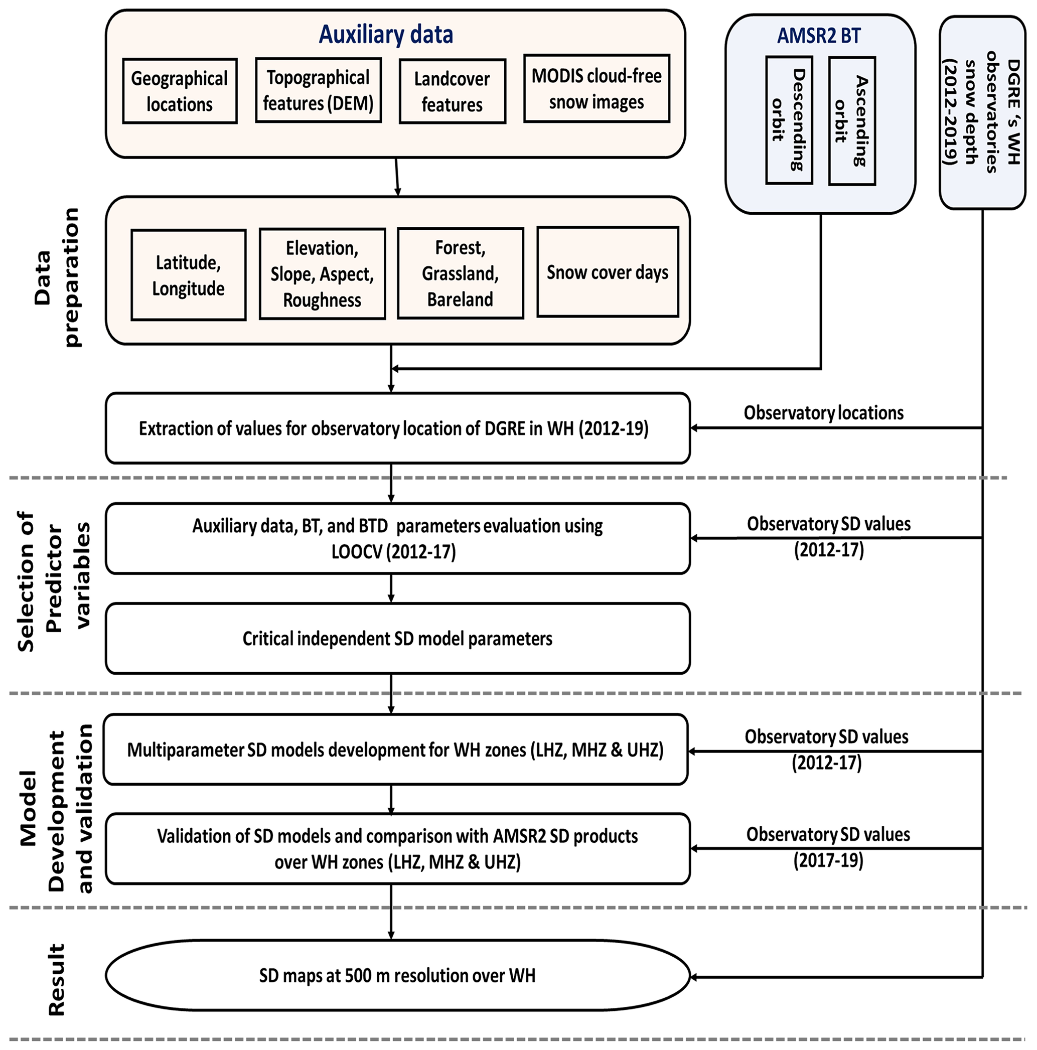
Different steps followed for developing and validating the multifactor SD model(s) are given in the following subsections from 3.1 to 3.5. The general outline of the methodology adopted is shown in Fig. 2.

Figure 2 Flowchart representing the methodology.

3.1 Data preprocessing

Different remote sensing datasets comprising PMW TB (from AMSR2), SRTM DEM, MODIS land cover product, and MODIS SCD are used in the current study. These products are natively present in different spatial resolutions and coordinate systems. Hence, all remote sensing datasets are processed using ArcGIS software to match the spatial extent, coordinate system, and spatial resolution. The brightness temperature and SD datasets downloaded from the JAXA portal use the Northern Hemisphere polar stereographic coordinate system and are present in the HDF5 format. These are reprojected to the WGS 1984 coordinate system and are converted to TIFF format with help of the format conversion tool developed by JAXA. Following that ArcGIS software is used for resampling the brightness temperature (BT) imagery to 500 m. No additional processing is carried out in the current work as the brightness temperature dataset acquired from JAXA is the level-3 product. The brightness temperature from each image for all stations is then retrieved programmatically using Python. The extracted TB data are used for calculating the BTD. The BTD is calculated between lower- and higher-frequency TB observations for each day during the study period.

Following the BTD calculation, the SRTM DEM product is re-projected, mosaicked, and resampled to 500 m spatial resolution. Different terrain parameters, such as slope, aspect, and surface roughness, are derived from the resampled DEM product. The SCD product is already available in 500 m spatial resolution. Therefore, it is processed only to match the extent and coordinate reference system (i.e., GCS-WGS 1984) of other datasets. Following the resolution and coordinate system matching process, for all DGRE observatory locations, the data from remote sensing products (i.e., TB, elevation, slope, ruggedness, geographical locations, and SCD) are extracted for the winter period from 2012–2013 to 2018–2019. It is known that the forest cover intercepts the upwelling radiation from the ground underneath the snowpack and causes uncertainty in the snow depth estimates of PMW SD models (Che et al., 2008). Therefore, the forest cover fraction has been calculated using the MODIS land cover type product (i.e., MCD12Q1) for a 10 km point buffer around each observatory site. The retrieved values are used to minimize the forest cover impact by dividing the brightness temperature observations by the value of non-forest fraction (i.e., 1 − forest fraction) for a given pixel as suggested by Foster et al. (1997).

In this study, the forenoon SD observations, descending pass AMSR2 TB data, terrain parameters (i.e., slope, aspect, ruggedness), geographical locations, and SCD are paired based on date and station location. These data are then checked for discrepancies such as missing values, incorrect values, and outliers. There are no missing values for AMSR2 TB, SRTM elevation, and SCD observations for the in situ stations over the WH region. However, samples containing any other discrepancies are removed. After data preprocessing, a total of ∼ 13 242 samples, with each sample comprising geographical location, TB, terrain parameters, and SCD, are retained. Using these samples, the data for the 5-year snow period, i.e., from 2012–2013 to 2016–2017, are used to develop multifactor SD algorithms for different zones of the WH region. The remaining 2 years of data of snow period, i.e., from 2017–2018 to 2018–2019, is used to compare and validate the multifactor SD model results.

3.2 Identification of dry snow pixel

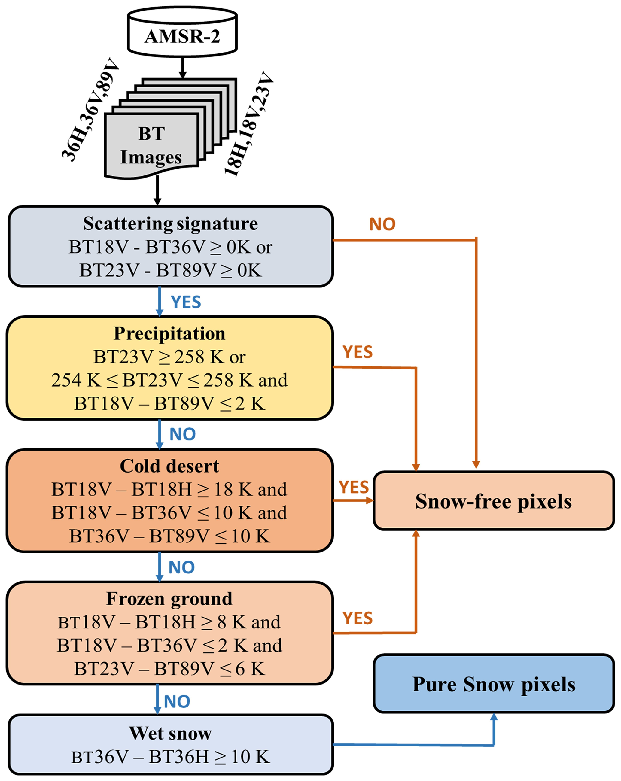
Along with snow cover, frozen ground, rainfall, and cold desert conditions affect the upwelling microwave emission from the earth's surface and impact PMW TB recorded by spaceborne sensors (Ferraro et al., 1996; Grody and Basist, 1996). Further, wet snow pixels and surface waterbodies cause PMW absorption and reduce volume scattering from snow grains (Stiles and Ulaby, 1980). Consequently, the inclusion of TB values from these pixels in the development and evaluation of the model results in large uncertainty in SD estimates (Tedesco et al., 2015; Dietz et al., 2012; Foster et al., 2005; Dong et al., 2005). Therefore, before developing SD algorithms, dry snow pixels must be segregated from other pixels. Grody and Basist (1996) have developed a decision tree to identify dry snow pixels from other scattering pixels using TB of different frequencies. Grody and Basist's (1996) decision tree makes use of different filters (see Fig. 3) based on the values of TB observations to separate snow from non-snow pixels. This study uses multifrequency AMSR2 TB data with Grody and Basist's (1996) decision tree to identify snow pixels.

Figure 3 Identification of pure snow pixels from AMSR2 TB using the decision tree.

3.3 Selection of multifactor SD model parameters

Many of the initial PMW SD models have relied on TB from 18 and 36 GHz channels for estimating SD (Chang et al., 1987; Saraf et al., 1999; Das and Sarwade, 2008; Kelly et al., 2003; Chang et al., 1997). However, these models have limitations in estimating shallow and deep snowpacks. The sensitivity of PMW TB to SD decreases once the SD reaches a threshold depth (Wang et al., 2019; Dai et al., 2018; Das and Sarwade, 2008; Kelly et al., 2003). TB values of higher frequencies (i.e., 36, 89 GHz) saturate before lower frequencies (i.e., 10, 18 GHz) as SD increases. The lower frequency (i.e., 10 GHz) has the potential to retrieve deep snow cover, while the higher frequency (i.e., 89 GHz) can provide shallow snow information (Kelly et al., 2003). Therefore, the inclusion of higher frequencies (i.e., 89 GHz) and lower frequencies (i.e., 10, 23 GHz) is investigated in many studies, which has resulted in improved SD estimates (Kelly et al., 2003; Wang et al., 2019; X. Xiao et al., 2020; Wei et al., 2021). Hence, PMW TB values of 10, 18, 23, 36, and 89 GHz are used in this study. Apart from single-channel SD, 40 combinations of TB, i.e., BTD of different frequencies and polarizations, are also considered. Terrain parameters (i.e., elevation, slope, aspect, surface roughness), location (latitude, longitude), land cover, and SCD also affect characteristics of snowpack and PMW TB (Saydi and Ding, 2020; Sharma et al., 2014; Wang et al., 2010; Ansari et al., 2019). Thus, overall, 57 parameters (i.e., TB – 10, BTD – 40, terrain parameters – 4, location – 2, SCD – 1) are considered in the process of SD model development. However, of the 57 parameters, it is likely that some parameters are redundant and do not necessarily add any value to the model. For example, TB values of 10H and 10V have a correlation of 0.9, and using both TB10H and TB10V is not useful and can cause additional problems due to multicollinearity. Further, the use of a large number of independent variables leads to a curse of dimensionality, which poses challenges in model development by decreasing the model's interpretability and increasing the computational time and resources, often leading to overfitting (Velliangiri et al., 2019; Obaid et al., 2019). These problems can be addressed by performing optimal parameter selection for model development (Chandrashekar and Sahin, 2014). Optimal parameter selection reduces the data dimensionality and eliminates irrelevant data from the original dataset.

This study considers data from the snow period between 2012–2013 and 2016–2017 of the entire WH region for optimal parameter selection. To select the necessary parameters for the SD model, all 57 parameters are used independently with in situ SD to develop single-parameter linear regression models. While developing these models, evaluation is carried out using the leave-one-out cross-validation (LOOCV) method (Webb et al., 2011) for screening necessary parameters. The LOOCV method is widely used by various researchers (Gusain et al., 2016; Joshi et al., 2017; Wang et al., 2019) to conduct the validation of models and assess the model's accuracy. In LOOCV, the observational dataset is used to create n number of regression models (n is number of samples). In each of the n models, a different testing sample is selected, and other observation samples are used to develop the regression model. The overall performance of the model is calculated by combining all predictions (for the omitted samples) from the n models. The accuracy of the models is calculated using the correlation coefficient (R) and RMSE. The results of LOOCV from the models developed with all 57 parameters (see Sect. 4.2) are analyzed to select the most valuable features for SD model development.

3.4 Development of SD models

This study implements four different regression models (i.e., linear, logarithmic, power, and reciprocal) to develop SD models. Different WH zones, i.e., LHZ, MHZ, and UHZ, have different topographic, environmental, and snowfall conditions. Hence, in this study, SD models are developed separately for each WH zone. Data from 2012–2013 to 2016–2017 are used for the development of the different SD models. Further, out of 57 parameters, 13 parameters are selected from the results of the LOOCV evaluation. These 13 parameters have a good correlation with in situ SD and are used in developing the multifactor SD models using four types of regression. The general form of the four types of regression models is given in Eqs. (7)–(10).

$$\begin{array}{}\text{(7)}& {\displaystyle }y={\mathit{\alpha }}_{\mathrm{1}}{x}_{\mathrm{1}}+{\mathit{\alpha }}_{\mathrm{2}}{x}_{\mathrm{2}}+\mathrm{\dots }+{\mathit{\alpha }}_i{x}_i+c,\text{(8)}& {\displaystyle }y={\mathit{\alpha }}_{\mathrm{1}}\ln x_{\mathrm{1}}+{\mathit{\alpha }}_{\mathrm{2}}\ln x_{\mathrm{2}}+\mathrm{\dots }+{\mathit{\alpha }}_i\ln x_i+c,\text{(9)}& {\displaystyle }y=c{x}_{\mathrm{1}}^{{\mathit{\alpha }}_{\mathrm{1}}}{x}_{\mathrm{2}}^{{\mathit{\alpha }}_{\mathrm{2}}}\mathrm{\dots }{x}_i^{{\mathit{\alpha }}_i},\text{(10)}& {\displaystyle }y={\mathit{\alpha }}_{\mathrm{1}}{\displaystyle \frac{\mathrm{1}}{x_{\mathrm{1}}}}+{\mathit{\alpha }}_{\mathrm{2}}{\displaystyle \frac{\mathrm{1}}{x_{\mathrm{2}}}}+\mathrm{\dots }+{\mathit{\alpha }}_i{\displaystyle \frac{\mathrm{1}}{x_i}}+c,\end{array}$$

where y is the ground-observed SD values; x₁, x₂, …, and x_i are the screened parameters; α₁, α₂, …, and α_i are the regression coefficients of the multiparameter models; c is the offset constant; and i represents the number of parameters.

3.5 Validation of SD model(s)

The multifactor SD models for different WH zones are validated using temporally independent in situ SD observations during 2017–2018 and 2018–2019. The accuracy of SD models' estimates is evaluated using standard regression metrics, i.e., R and RMSE. Additionally, the efficacy of the proposed multifactor SD models is analyzed by comparing the accuracy of the multifactor model with regional (Das and Sarwade, 2008; Singh et al., 2020) and heritage (Chang et al., 1987) SD models for different ranges of the WH region. The SD models of Chang et al. (1987), Das and Sarwade (2008), and Singh et al. (2020) are given in Eqs. (11), (12), and (13), respectively.

The comparison is carried out by estimating SD from all these stated models using the validation data present between 2017–2018 and 2018–2019.

$$\begin{array}{}\text{(11)}& {\displaystyle }{\mathrm{SD}}_{\text{Chang et al. (1987)}}=\mathrm{1.59}\times (\mathrm{TB}\mathrm{18}\mathrm{H}-\mathrm{TB}\mathrm{36}\mathrm{H}),\text{(12)}& {\displaystyle }{\mathrm{SD}}_{\text{Das and Sarwade (2008)}}=\mathrm{3.16}\times (\mathrm{TB}\mathrm{18}\mathrm{H}-\mathrm{TB}\mathrm{36}\mathrm{H})+\mathrm{24.25},\text{(13)}& {\displaystyle }{\mathrm{SD}}_{\text{Singh et al. (2020)}}=-\mathrm{7.58}\times (\mathrm{TB}\mathrm{18}\mathrm{V}-\mathrm{TB}\mathrm{36}\mathrm{V})+\mathrm{233.71},\end{array}$$

where TB denotes the brightness temperature values, 18 and 36 indicate the frequency of TB (in GHz), and V and H are the vertical and horizontal polarization, respectively.

Apart from the aforementioned comparative analysis, a random sample image from the study area for a single day (3 February 2019) is taken. Then, the estimated SD over the selected area using the multifactor SD model(s) is spatially compared with AMSR2 operational products (see Sect. 4.5). This spatial comparison helps in understanding how the developed multifactor SD model(s) differs from the AMSR2 operational SD products in representing SD information over the WH region. The magnitude of in situ SD, terrain parameters, and SCD can significantly affect the accuracy of the PMW SD model in the study region. Therefore, the accuracy of operational AMSR2 SD products and multifactor SD models with respect to varying ground SD, topographic elevation, and SCD is determined in different WH zones (see Sect. 4.6).

4 Results and analysis

The insights from the analysis of in situ SD observations in WH zones are reported in Sect. 4.1. Following that, the results from the LOOCV evaluation of multiple parameters are given in Sect. 4.2. The outcomes from the accuracy assessment and comparison of different PMW SD estimates are described in Sect. 4.3 and 4.4, respectively. The spatial comparison of the high-resolution SD map from the multifactor model and AMSR2 products is shown in Sect. 4.5. In Sect. 4.6, the analysis of multifactor SD model performance with respect to different parameters is detailed.

4.1 Spatial analysis of the in situ SD observations in WH ranges

The mean of in situ SD at each of the 43 DGRE stations is estimated for the winter period (October to March) during 2012–2013 to 2018–2019 (see Fig. 4). The results indicate that during the data period, the mean SD values varied between ∼ 11 cm (elevation: 1664 m) and ∼ 256 cm (elevation: 3160 m) in the LHZ, ∼ 21 cm (elevation: 3250 m) and ∼ 136 cm (elevation: 4950 m) in the MHZ, and ∼ 49 cm (elevation: 3250 m) and ∼ 365 cm (elevation: 5995 m) in the UHZ. The analysis also demonstrates that out of 43 manual stations, 4 stations have a mean SD between 11 and 50 cm, 18 stations have a mean SD between 50 and 100 cm, 7 stations have a mean SD between 100 and 150 cm, 5 stations have mean SD between 150 and 200 cm, and the remaining 4 have mean SD >200 cm during the data period. Further, it is observed that out of nine stations that have a mean SD greater than 150 cm, five are present in the UHZ.

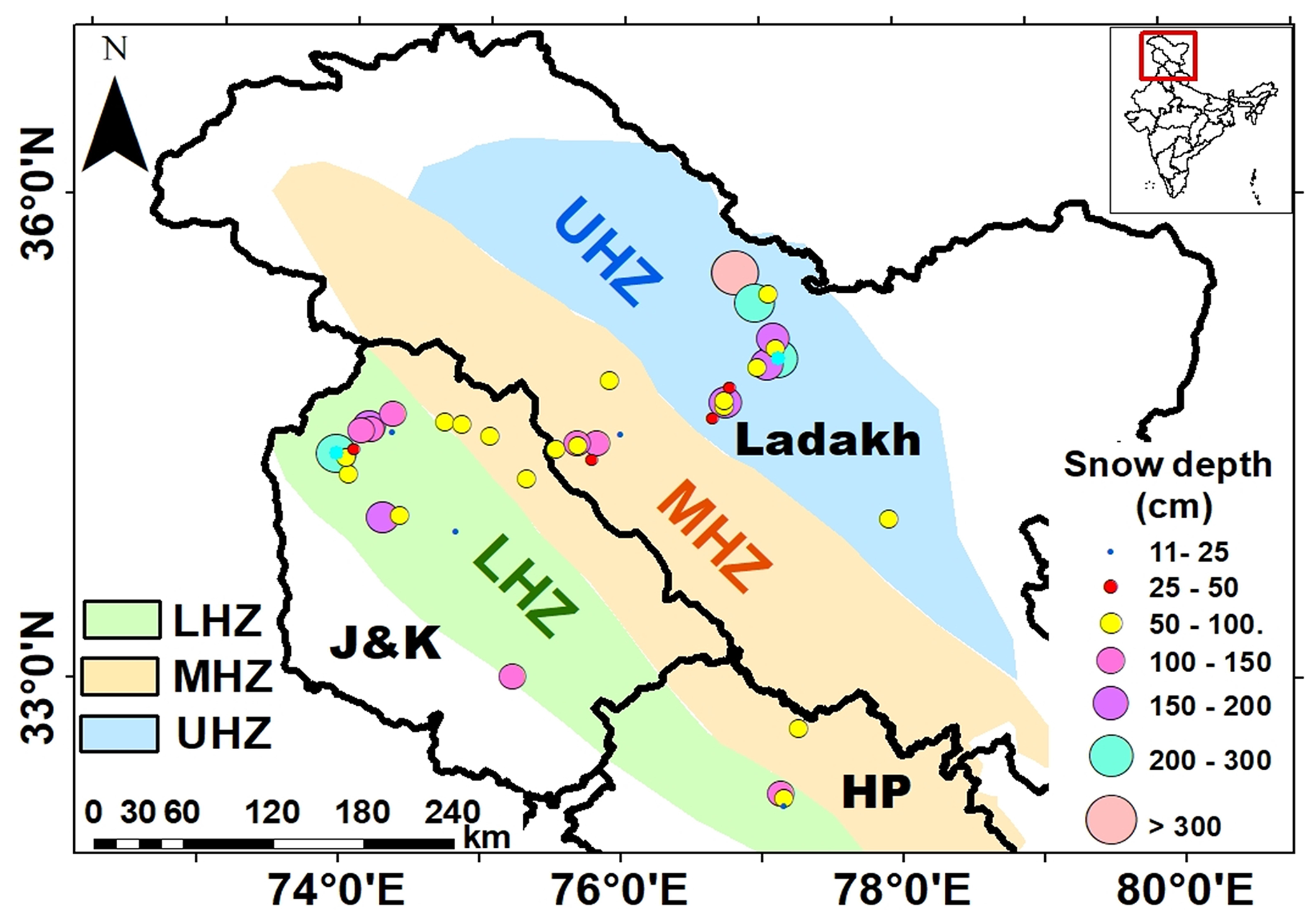
Figure 4 Spatial distribution of mean SD in WH zones along DGRE stations during 2012–2019 (October to March months) (Note: J&K is Jammu and Kashmir, HP is Himachal Pradesh).

The overall analysis of in situ SD measurements indicates the mean and standard deviation (μ ± σ) are observed as ∼ 121.5 cm ± 122.5 cm in the LHZ, ∼ 85.9 cm ± 83.5 cm in the MHZ, and 176.6 cm ± 208.9 cm in the UHZ. A higher mean SD is observed in the UHZ compared to the other two ranges. A total of 95 % of overall SD values in the LHZ are below 350 cm, with the remaining 5 % having SD between 350 and 650 cm. However, in the MHZ and UHZ, 95 % of total SD observations are below 200 and 500 cm, respectively, with the remaining 5 % ranging between 200 and 500 cm and 500 and 2030 cm.

4.2 SD parameters screening and evaluation over the WH region

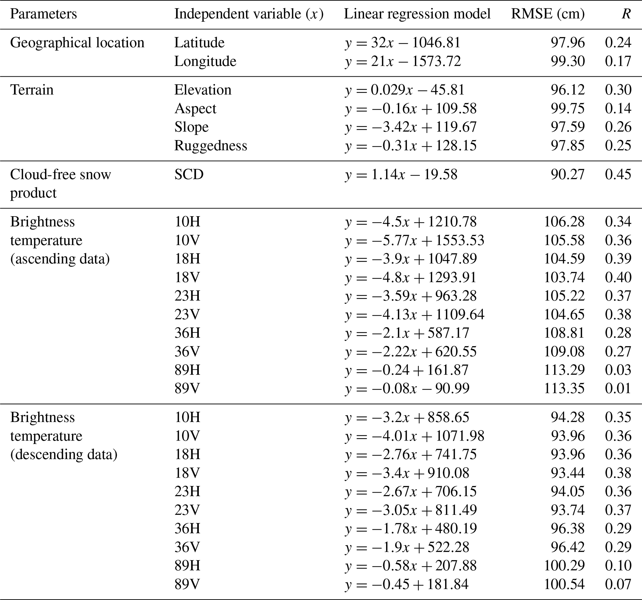
The expressions for linear regression models developed with each parameter and regression metric, i.e., RMSE and R results obtained from LOOCV analysis, are shown in Table 3. In terms of geographical location, latitude has a higher correlation (i.e., 0.24) and lower RMSE (97.96 cm) than longitude. Among the terrain parameters, SCD has the highest R (i.e., 0.45) and the lowest RMSE (i.e., 90.27 cm) and is followed by elevation (R=0.30 and RMSE = 96.12), slope (R=0.26 and RMSE = 97.59), and ruggedness (R=0.25 and RMSE = 97.85), making it highly important for the development of multifactor SD models. The SD models built with TB observations from descending orbital passes have a relatively higher correlation and lower RMSE than those from ascending pass TB data when analyzed with in situ SD. This is mainly because descending orbital passes occur in the morning time with no melting of snow; however, ascending orbital passes occur in the afternoon time with substantial melting of snow in the study area. Therefore, only descending pass TB observations are used in the study.

Table 3 Results of LOOCV evaluation for SD models developed using single parameters.

y= SD (cm).

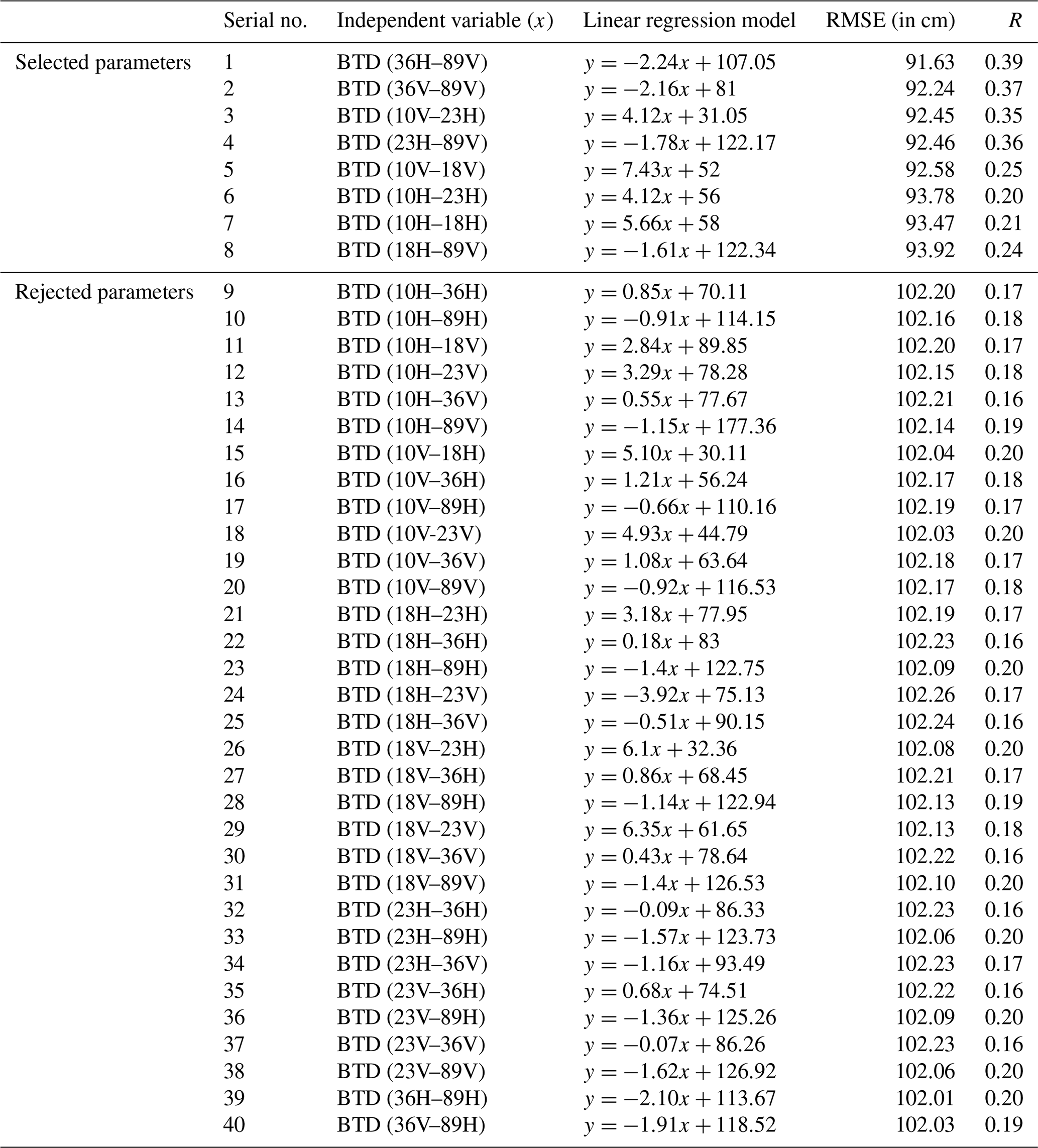
Apart from the single-channel PMW TB, 40 different combinations of descending pass orbital BTDs are tested using linear regression (in the LOOCV approach). The selected and rejected BTD parameters with their RMSE and R with the in situ SD are shown in Table 4. The selected parameters have the lowest RMSE and highest correlation, and they pass the F test at a significance level of 0.001. It is observed that descending pass BTD models exhibit higher correlation and accuracy metrics compared to single-channel descending pass models. From the overall results (R, RMSE), descending pass BTD parameter-based SD models have higher R (0.24 to 0.39) and lower RMSE (91.63 to 93.92 cm) compared to single-channel TB-based SD models, which have R values of 0.07 to 0.35 and RMSE values of 93.44 to 100.54 cm. Therefore, different BTD data from descending passes (see Table 4) are selected instead of single-channel TB to develop multifactor SD models. Along with the eight descending BTD parameters (BTD of 10H18H, 10H23H, 18H89V, 36H89V, 36V89V, 23H89V, 10V89V, and 10V23H, where 10, 18, 23, 36, and 89 represent the frequency (in GHz), and H and V represent horizontal and vertical polarization, respectively), three terrain parameters (elevation, slope, ruggedness), latitude, and SCD are used to develop multifactor PMW SD models for the three WH ranges.

Table 4 BTD SD model (with descending observations) relation with SD and evaluation using LOOCV method.

Note: y= SD (cm).

4.3 Evaluation and comparison of different multifactor SD models in WH zones

The details of the developed models are given in Table 5. The results from the regression analysis indicate multifactor SD models developed with a power regression approach have a better fit with the in situ data and outperformed other regression models with R (RMSE in cm) values of 0.62 (49.17), 0.78 (37.72), and 0.76 (55.12) in the LHZ, MHZ, and UHZ, respectively.

Table 5 Multifactor SD model regression coefficient for WH zones during 2012–2017 (October to March).

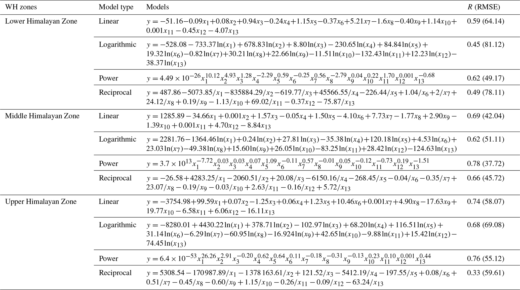
Note: in Table 5, x₁ to x₅ are latitude, elevation, slope, ruggedness, and SCD, respectively; x₆ to x₁₃ are the BTD of 10H18H, 10H23H, 18H89V, 36H89V, 36V89V, 23H89V, 10V89V, and 10V23H, respectively; V is the vertical polarization; H is the horizontal polarization; and 10, 18, 23, 36, and 89 are the frequency (in GHz) of the corresponding BT channels.

The developed multifactor models in each WH zone are evaluated (with R and RMSE metrics) using temporally independent data from 2017–2018 to 2018–2019. Comparison of the four types of multifactor regression models in the LHZ, MHZ, and UHZ is carried out with the help of the Taylor diagram (see Fig. 5). The R and RMSE (in cm) for the metrics of power, linear, logarithmic, and reciprocal models in different WH zones are given in Fig. 5 and Table 6. The results from the comparison indicate that in all WH zones, the multifactor SD model developed using power regression has exhibited higher accuracy, i.e., better correlation and lower RMSE compared to the models built using linear, logarithmic, and reciprocal regression approaches. Therefore, in each WH zone, the multifactor SD model from power regression is used to estimate PMW SD at 500 m spatial resolution.

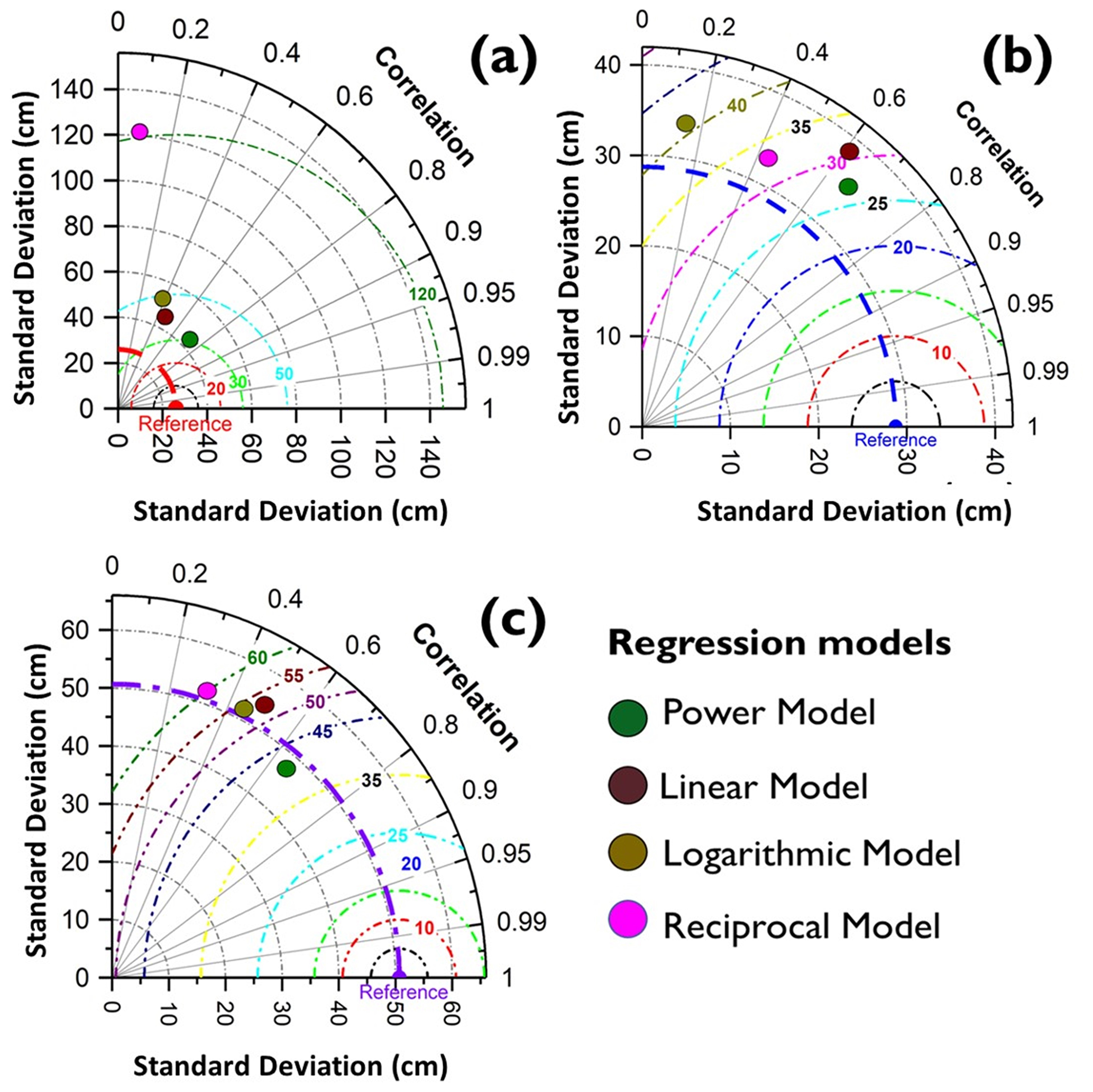
Figure 5 Taylor diagram for the evaluation of multifactor SD models during 2017–2019 for (a) the LHZ, (b) the MHZ, and (c) the UHZ.

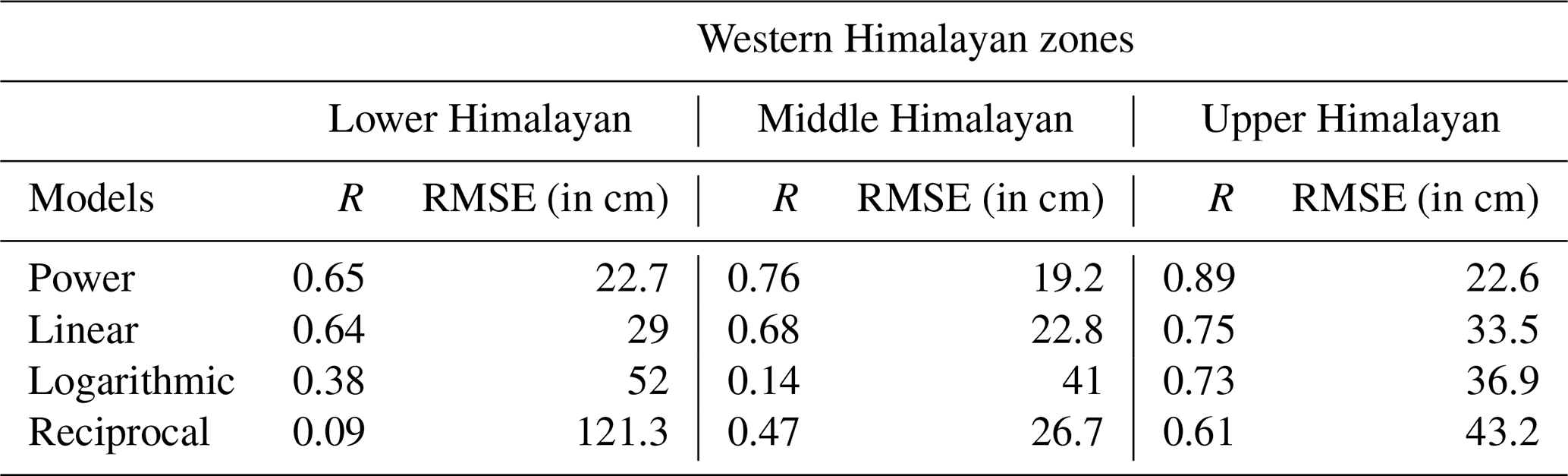
Table 6 Comparative analysis of multifactor SD models during 2017–2019 for WH zones.

4.4 Comparative analysis of multifactor and other SD models in different zones of the WH region

In order to compare the performance of different SD models in the WH region, the SD values are estimated using different models with the help of PMW and other auxiliary data during the study period (i.e., 2017–2018 to 2018–2019). Different models used in the comparative analysis are the multifactor SD model(s) from this study, regional SD models of the WH region (i.e., Das et al., 2008; Singh et al., 2020), and the heritage SD model provided by Chang et al. (1987). The estimated SD from each model is compared with in situ SD observations within the respective WH zones to understand the accuracy of SD retrievals. Singh et al.'s (2020) model is proposed only for the MHZ. Therefore, it is not used for SD estimation in the LHZ and UHZ when doing comparative analysis.

In the LHZ, both Chang's model and Das's model have poor correlation with in situ SD and have shown RMSEs (R) of 39.51 (−0.16) and 49.66 (−0.14) (see Fig. 6), whereas the proposed multifactor SD model has shown a good correlation with RMSE (R) of 32.87 (0.75). In the MHZ, Chang et al. (1987), Das et al. (2008), and Singh et al. (2020) have exhibited poor correlation with in situ SD with R values of 0.22, 0.21, and −0.22, respectively, whereas the proposed multifactor SD model has shown a good correlation with in situ SD with an R value of 0.65 (see Fig. 6). The RMSE is observed to be 36.32, 49.82, and 119.79 cm for the Chang et al. (1987) model, Das et al. (2008) model, and Singh et al. (2020) model, respectively. The proposed multifactor SD model has shown good accuracy with a lower RMSE of 27.21 cm compared to other SD models. The SD model proposed by Singh et al. (2020) for the MHZ is developed using data from a single observatory location. Hence, the Singh et al. (2020) model cannot represent the spatial variability in SD and shows significant errors with higher bias.

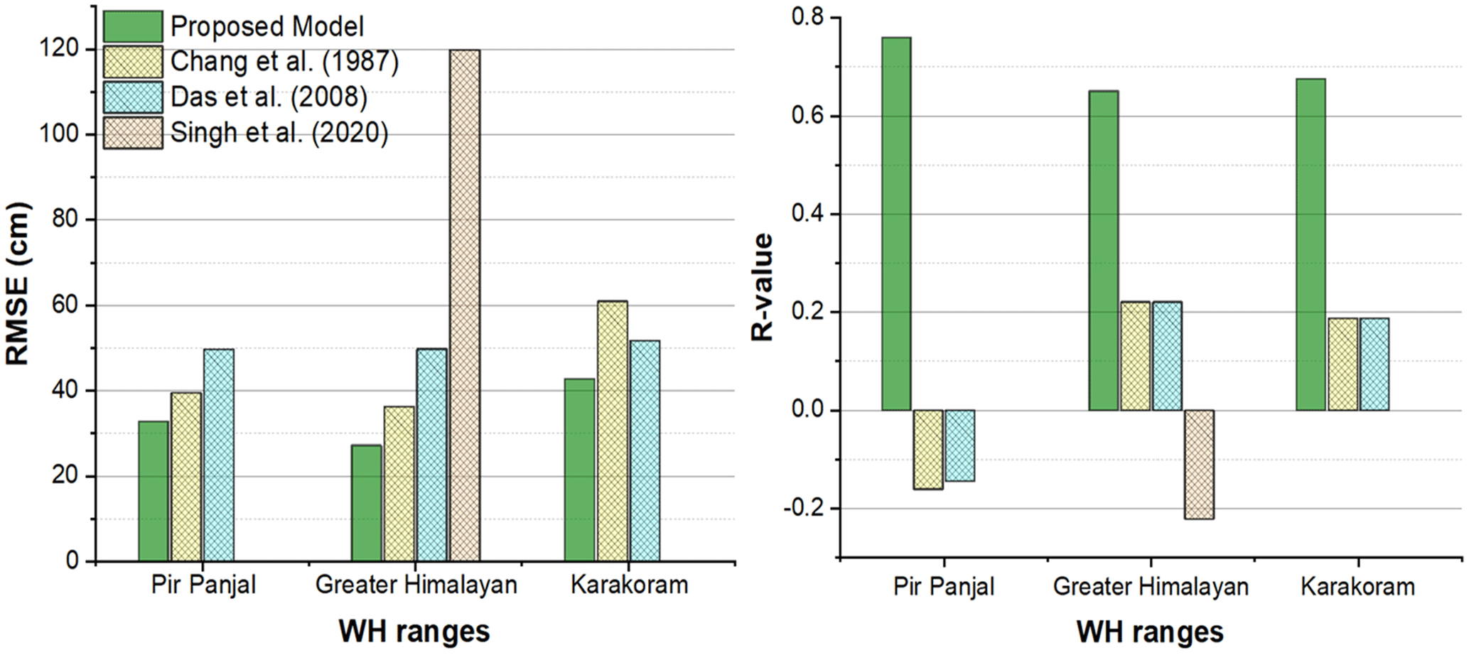
Figure 6 Comparison of model-estimated and field-observed SD values in the LHZ (Pir Panjal), MHZ (Greater Himalayan), and UHZ (Karakoram) during 2012–2019 (October to March).

Similar to the results observed in the LHZ and MHZ, the Chang et al. (1987) model and Das et al. (2008) model have shown a poor correlation in the UHZ with R values of 0.18 and 0.19, respectively. In comparison, the multifactor SD model has shown a good correlation with an R value of 0.67 (see Fig. 6). The RMSE values are observed to be 60.95, 51.74, and 42.81 cm for the Chang et al. (1987) model, Das et al. (2008) model, and proposed multifactor SD model in the UHZ. Overall results from the comparative analysis indicate that in each WH zone, the multifactor SD model has higher accuracy with good correlation (i.e., R) and lower errors when compared with other models. Further, the developed model has exhibited better accuracy metrics in the MHZ compared to other WH zones. The mean SDs observed during the study period (i.e., 2017–2018 to 2018–2019) in Pir Panjal and UHZ are higher than the mean SD of the MHZ. Further, the LHZ has a forest canopy which can affect the PMW TB observations, whereas, in the MHZ, most of the region is devoid of forest vegetation except for some patchy grass vegetation. Hence it is expected that an increased error for SD models in the LHZ and UHZ compared to the MHZ will be observed.

4.5 Spatial comparison of SD from multifactor model and operational AMSR2 SD products: a case study

The spatial comparison of SD maps from AMSR2 SD products and the multifactor SD model is performed to understand the improvement in the AMSR2 multifactor SD model over the operational AMSR2 SD products in the WH region. For this purpose, the SD maps of operational AMSR2 SD products and the multifactor SD model for WH zones for 3 February 2019 are considered (see Fig. 7). The SD spatial map at 500 m resolution for the WH zones is generated using the multifactor SD model (see Fig. 7d). The AMSR2 ascending SD product, i.e., AMSR2_A (see Fig. 7b), and descending SD product, i.e., AMSR2_D (see Fig. 7c), of the same region for the given day at 10 km resolution are also prepared.

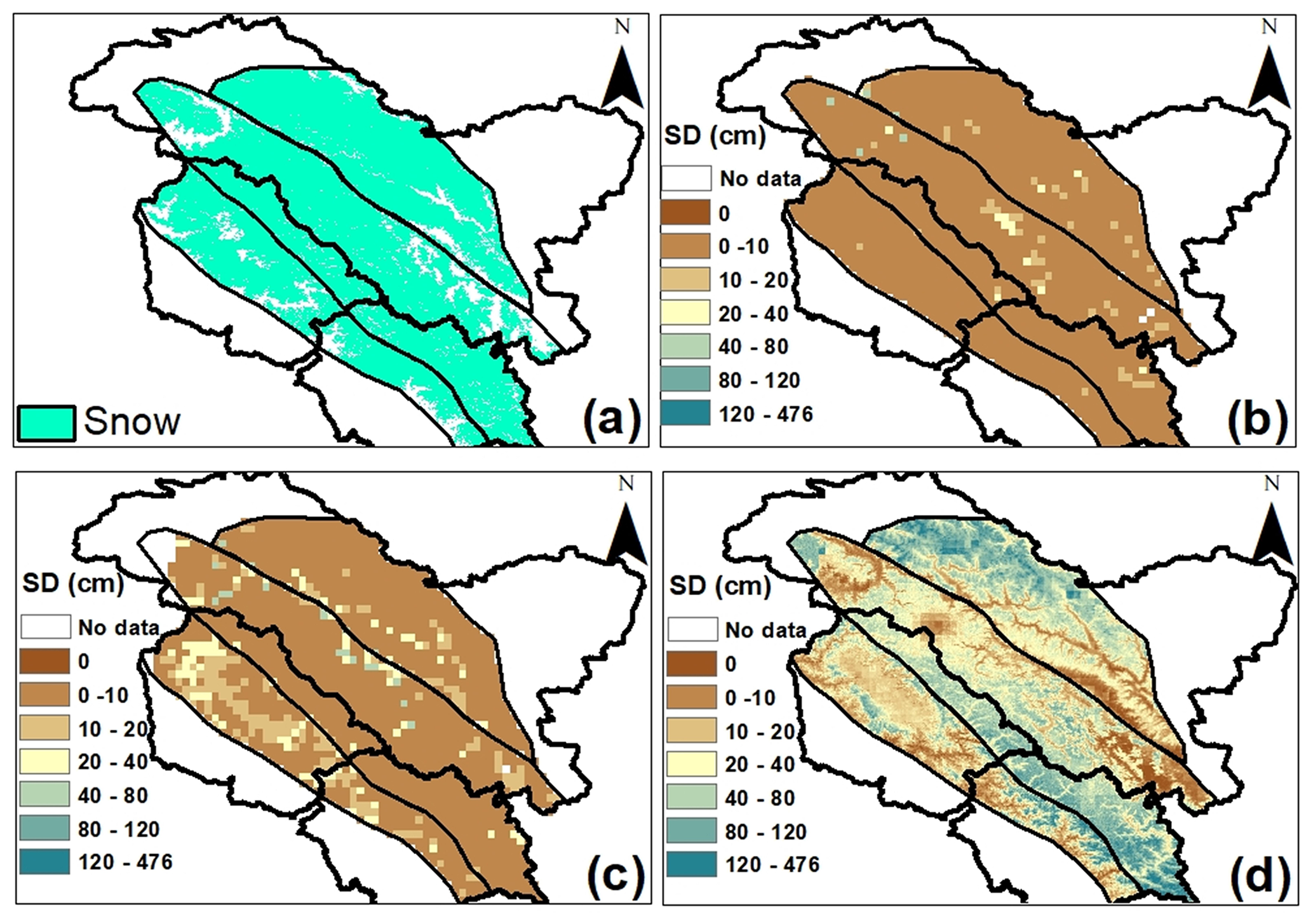
Figure 7 Spatial map of SD variation on 3 February 2019. (a) MODIS SCA, (b) AMSR2_A SD product map at 10 km, (c) AMSR2_D SD product map at 10 km, and (d) multifactor SD model map at 500 m.

According to MODIS-derived SCA at 500 m resolution (see Fig. 7a) and DGRE observatories' in situ SD information, this is snow cover with varying thickness on 3 February 2019 in WH zones. However, in both the AMSR2 SD products, i.e., AMSR2_A and AMSR2_D, the majority of pixels have zero SD value, resulting in the underestimation of SD information by AMSR2 products. The maximum SD values observed in different products are as follows: AMSR2 ascending SD, 58 cm; AMSR2 descending SD, 78 cm; multifactor SD model, 476 cm. The multifactor SD model shows high heterogeneity in SD across the selected region in WH zones compared to AMSR2 SD products. Further, the multifactor SD model offers good detail about snow cover and provides SD data in the region at a high resolution of 500 m.

4.6 Comparison of performance of multifactor SD product with operational AMSR2 SD product

Though regions with higher mean SD (i.e., LHZ, UHZ) have a higher error than regions with a lower mean SD (i.e., MHZ), it is important to assess how the SD products' accuracy varies with changes in in situ SD. Hence, Sect. 4.6.1 analyzes the operational AMSR2 SD products and AMSR2 multifactor model performances in different SD classes. Further, it is also essential to understand how the model's accuracy is affected with respect to different auxiliary parameters, i.e., topographical and land cover parameters. Therefore, the model accuracy is evaluated with respect to different topographical and land cover parameters, and the results are presented in Sect. 4.6.2.

4.6.1 Analysis of operational AMSR2 SD products and multifactor SD model in different SD classes

In each WH zone, the AMSR2 SD products and multifactor SD model estimates are grouped into five SD classes, i.e., 0–25, 25–50, 50–75, 75–100, and >100 cm based on in situ SD observations during 2017–2018 to 2018–2019. Along with the multifactor SD, the operational AMSR2 SD product (i.e., from both ascending and descending pass data) is also analyzed in the SD classes by comparing it with in situ SD observations. RMSE of each SD class is calculated to evaluate the accuracy of SD estimates. Other models (i.e., Chang et al., 1987; Das et al., 2008; and Singh et al., 2020) were not considered in this analysis as they were not operational SD models. The effect of variation in ground SD on the accuracy of the AMSR2 multifactor SD model and AMSR2 SD products is shown in Table 7.

Table 7 RMSE of operational AMSR2 SD products and the proposed multifactor SD model across different WH zones in different in situ SD classes.

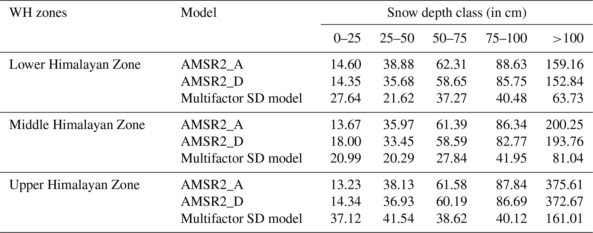
The results indicate that the magnitude of RMSE of AMSR2 SD products and the multifactor SD model increased with an increase in SD. When in situ SD <25 cm, AMSR2 SD products have shown relatively lower error in all three zones compared to the developed multifactor SD model. However, the observed error in this class (i.e., 0–25 cm) is still large and varies between 11–15 cm in the AMSR2 SD product and 14–27 cm in the multifactor SD model across the three zones, whereas for classes with in situ SD >25 cm, the proposed multifactor SD model has a lower RMSE than both AMSR2 products in all the zones of the WH region. This analysis clearly shows that for shallow snow regions in the WH region, operational AMSR2 products can be used. However, the AMSR2 SD products show a large error for deep and moderate snow regions. In the WH region, out of 43 stations, only four stations have a mean SD <25 cm, and for the remaining stations, the mean in situ SD was more than 25 cm during the study period. Hence AMSR2 SD products are less useful for spatial monitoring of SD in the WH region. Though the developed AMSR2 multifactor model has shown higher error when in situ SD <25 cm, it is more useful for the WH region as the RMSE is lower when SD >25 cm.

Overall, the multifactor SD model in the MHZ has a low RMSE compared to the LHZ and UHZ in all SD classes. This could be due to prevailing dry snow conditions, lower mean SD, and the absence of forest in this range, which can favor the PMW SD algorithms to retrieve better SD estimates from PMW TB, whereas higher temperatures, moist snow conditions, forest vegetation in the LHZ, and deep snow conditions in both the LHZ and UHZ can negatively affect the accuracy of the AMSR2 multifactor SD model in these regions by affecting the TB observations.

4.6.2 Multifactor model performance analysis with respect to auxiliary parameters

Among all the factors considered in the AMSR2 multifactor SD model development, elevation and SCD have good heterogeneity across the stations in each WH zone. The other terrain factors, such as slope and land cover, do not have much variation and are similar for many of the stations within a WH zone (see Fig. 8). Though a large variation in land cover is observed across the entire WH region, in the LHZ the majority of stations are surrounded by forest cover, whereas in the MHZ, stations are mainly over grassland and barren land. The UHZ is devoid of vegetation, and all stations are present over barren land and glaciers. Thus, the variation in land cover within a range is not significant. Therefore, in this section, only the effect of varying elevation and SCD on the accuracy of SD from the AMSR2 multifactor SD model and operational AMS2 SD products is evaluated.

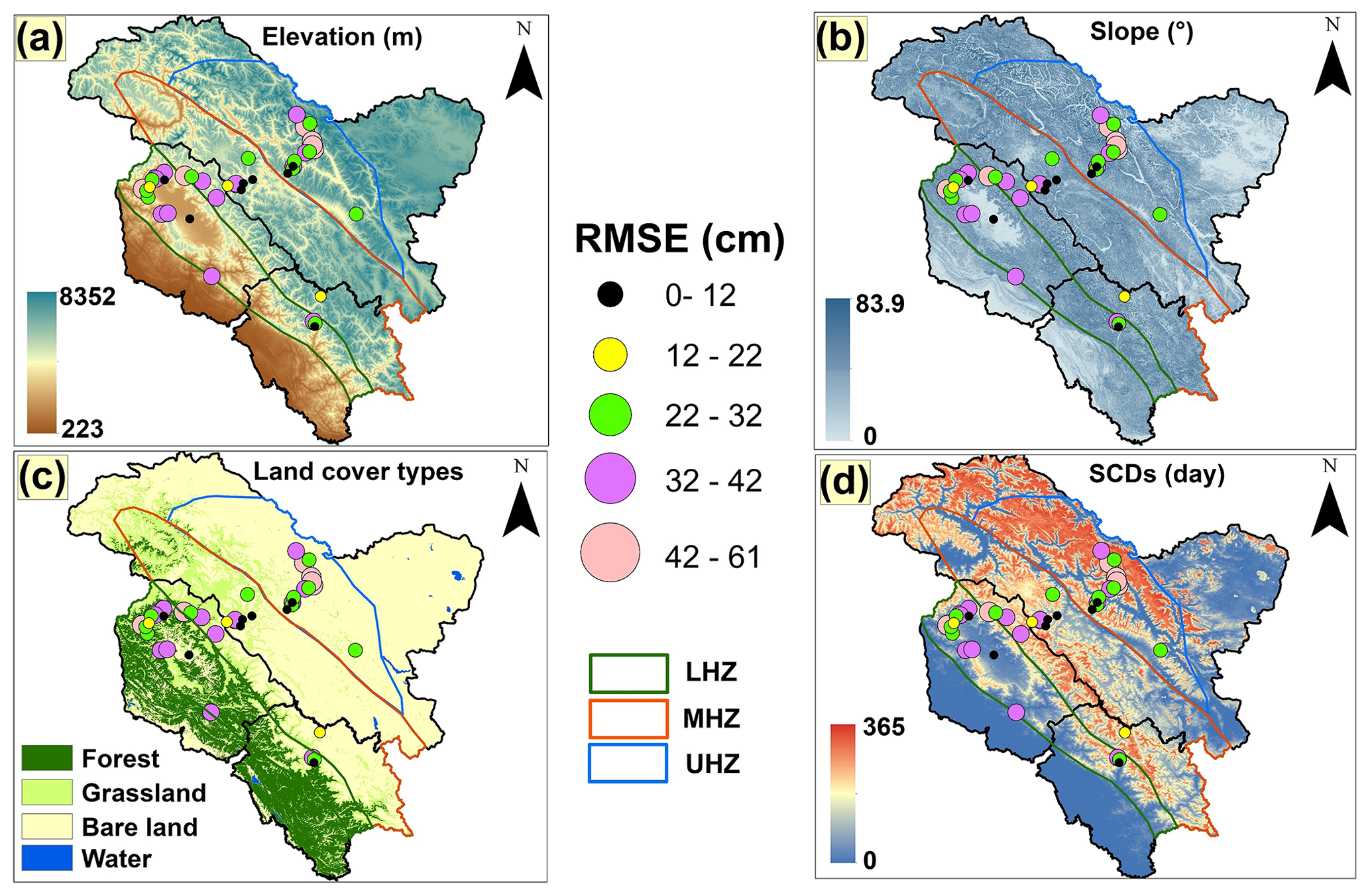
Figure 8 Spatial distribution of RMSE of the multifactor SD model for varying (a) elevations, (b) slopes, (c) land cover types, and (d) SCD among the 43 ground stations.

Slope and SCD are divided into different classes considering the overall variation in the WH region. Within these classes, the SD retrievals from the AMSR2 products and multifactor model are compared with in situ SD measurements during the winter period between 2017–2018 and 2018–2019. The accuracy of model estimates in each class is evaluated by calculating RMSE (see Table 8). The RMSE associated with each station for different factors (i.e., elevation, slope, SCD, and land cover) is depicted in Fig. 8. The results indicate that in the LHZ and UHZ, with an increase in elevation, RMSE increased for both AMSR2 products and the multifactor model, whereas in the MHZ, there is no specific trend in the variation in accuracy with respect to elevation. The RMSE (in cm) variation across all elevation classes for the multifactor SD model and AMSR2 ascending and AMSR2 descending SD products in different WH regions is as follows: LHZ, 21.38–47.27, 23.05–113.21, and 18.44–93.72 cm; MHZ, 17.82–54.79, 39.10–107.72, and 37.98–103.38 cm; UHZ, 11.73–126.13, 17.71–188.67, and 19.50–182.12 cm. Though overall RMSE variation is high across the different elevation classes, both AMSR2 SD products have similar RMSEs for any given elevation class within each WH zone. However, the multifactor SD model has lower RMSE than both AMSR2 SD products for elevation classes across the three WH zones. Other than elevation, the amount of snowfall and snow conditions vary widely with SCD across the different WH zones. This can lead to varying accuracy trends in SD retrievals for a given factor in different WH zones.

Table 8 RMSE (cm) variation in AMSR2 SD products and the multifactor SD model for different elevations, as well as SCD classes across three WH zones (for snow period during 2017–2018 to 2018–2019).

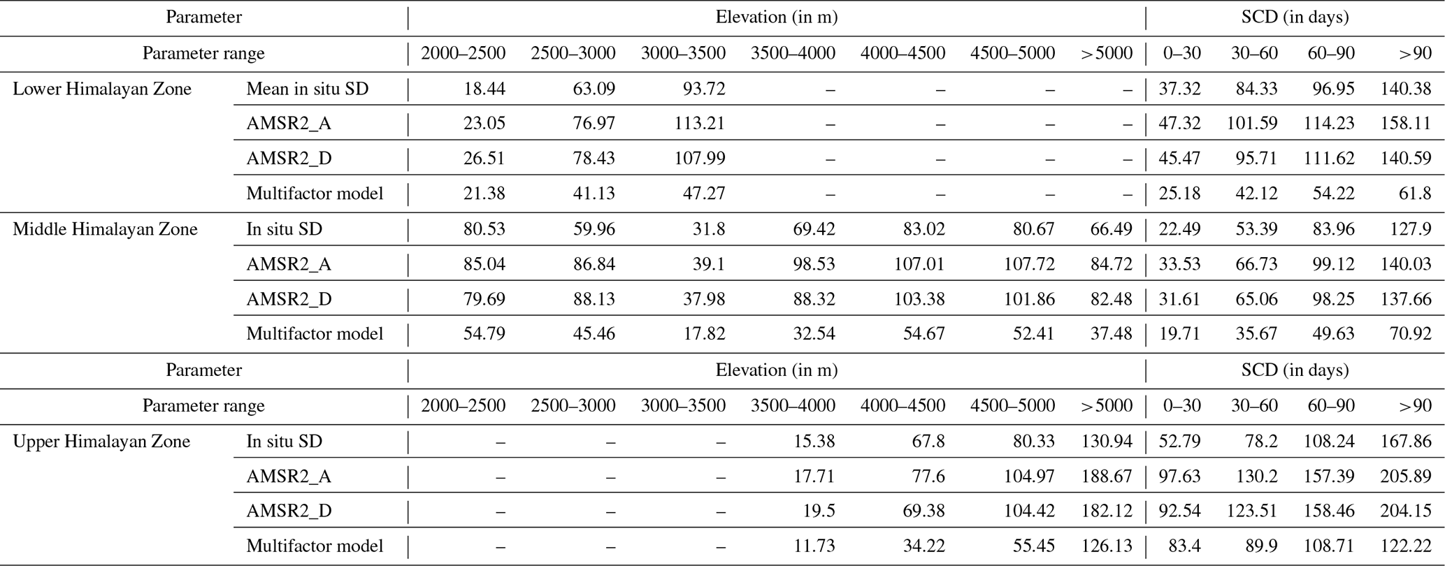
The SD generally increases with an increase in SCD, affecting the PMW SD retrieval from different models. Across all WH regions, the RMSE values of the AMSR2 ascending and AMSR2 descending SD products and the multifactor SD model increased with an increase in SCD. However, the RMSE of the multifactor SD model is significantly low compared to the AMSR2 SD products in all SCD classes in each WH zone. The SCD variation at the end of the snow year (30 September 2013), along with RMSEs in different stations calculated for the time period, i.e., 2017–2018 to 2018–2019, is represented in Fig. 8d. The RMSE variation associated with SCD classes for the multifactor SD model, AMSR2 ascending product, and AMSR2 descending product in different WH ranges are as follows: LHZ, 25.18–61.80, 47.32–158.11, and 45.47–140.59 cm; MHZ, 19.71–70.92, 33.53–140.03, and 31.61–137.66 cm; UHZ, 83.40–122.22, 97.63–205.89, and 92.54–204.15 cm.

5 Discussion

The Indian WH region has the highest mountain peaks in Asia that separate the plane regions of the Indian subcontinent from the Tibetan Plateau with a mean elevation of ∼ 3116 m a.m.s.l. The discussion about the performance of SD models and factors affecting the multifactor SD model is given in Sect. 5.1 and 5.2, respectively.

5.1 SD models' performance

Four multifactor SD models are developed for each WH zone using different regression approaches (i.e., linear, logarithmic, reciprocal, and power). These models are compared with regional SD models, Chang's SD model, and operational AMSR2 SD products. The overall analysis of the results indicates that the power-regression-based multifactor SD model has higher accuracy compared to other multifactor SD models, regional approaches, Chang's model, and AMSR2 SD products in all WH regions. However, AMSR2 SD products have shown comparable to better accuracy (i.e., similar to the multifactor SD model) under shallow snow conditions (SD <25 cm). Nevertheless, once SD exceeds 25 cm, the performance of AMSR2 SD products declined considerably (see Table 8). Further, AMSR2 SD products have a large amount of missing data over the WH region, highlighting its poor utility for various regional applications. The regression modeling approach attempts to find a better fit by optimizing the loss function, i.e., mean error. Over the WH region, the majority of the observations have SD >25 cm. Therefore, understandably the model estimates are better in higher-SD regions compared to shallow-SD regions.

The proposed model has an overall positive bias with overestimated SD values for shallower SD and underestimation in the case of higher-SD observations. The bias for the LHZ, MHZ, and UHZ for the proposed model is 4.5, 2, and 6.3 cm, respectively, whereas the bias for the legacy model and other regional models is considerably higher with significant overestimates in the lower depth values and underestimates in higher-depth regions. Further, it must be emphasized that these models have very poor correlation with the in situ snow depth and the SD estimates mainly confined in a range irrespective of the magnitude of the ground snow depth observation values.

In general, with an increase in SD, the accuracy of multifactor models declined in all WH zones. However, the accuracy of developed multifactor SD models is distinct for a given SD class in different WH zones. This is because the spatial distribution of snowfall and snow characteristics (i.e., SD, snow wetness, density) are not uniform at different geographic locations of observatories distributed across the three WH zones. The SD model developed in the MHZ has shown better accuracy metrics than those developed for the LHZ and UHZ.

The topographical parameters in the WH region play a vital role in affecting the local climate as well as snow distribution. The inherent weakness of PMW TB in capturing deeper snowpack thickness is overcome to a certain extent by considering SCD in model development. Thus, the overall improved performance of the multifactor model over the previously developed models and AMSR2 products can be attributed to the consideration of topographical parameters and SCD in the model development. Further, a combination of multiple lower- and higher-frequency TBs is considered in the model for capturing both deeper and shallower snowpack thickness. Different factors affecting the performance of the multifactor SD model are discussed in Sect. 5.2.

5.2 Factors affecting the performance of multifactor SD model

A total of 57 parameters comprising multifrequency PMW TB, BTD, terrain parameters, and SCD are screened using LOOCV to determine the suitable factors to develop the PMW multifactor SD model. Finally, the SD algorithm is developed only using the selected parameters, i.e., geographical location parameters (latitude), terrain parameters (elevation, slope, and ruggedness), SCD, and BTDs (36H89V, 36V89V, 10V23H, 23H89V, 10V18V, 10H23H, 10H18H, and 18H89V). In the present study, different combinations of frequencies in vertical and horizontal polarization have been used to estimate shallow to deep snow across different zones of the WH region. Only descending pass PMW observations are employed in this study to avoid the problems pertaining to wet snow, which is more prominent during the ascending pass. Among the different factors (i.e., other than PMW data) evaluated using LOOCV, SCD has shown a relatively strong correlation (i.e., R=0.45) with in situ SD observations. Higher SCD generally indicates longer snow persistence which leads to an increase in snow accumulation, whereas shorter SCD indicates the absence/melt of snow, which leads to lower SD.

Apart from SCD, terrain parameters, i.e., elevation and slope, have an impact on the spatial distribution of SD within an area (Saydi and Ding, 2020; Trujillo et al., 2007; Sharma et al., 2014) and have shown a moderately better correlation with in situ SD with R values of 0.30 and 0.26, respectively (see Table 3). Further, the topographic conditions can affect the reallocation of PMW radiation due to variations in the direction of polarization and local incidence angles (You et al., 2011), altering the TB values. The higher-elevation regions (i.e., UHZ) of the Western Himalaya experience cold conditions, which aids snow in accumulating. Therefore, the snowfall is preserved for most of the winter in higher mountain areas of the MHZ and UHZ, leading to higher SD in these regions. The accuracy of PMW SD models varies with the magnitude of in situ SD, as evident from the current study, as well as from many previous studies (X. Xiao et al., 2020; L. Xiao et al., 2020; Dai et al., 2018). However, there are many other factors (such as land cover, snow wetness, and grain size) that can affect the accuracy of SD retrievals (Dong et al., 2005; Foster et al., 2005; Tedesco et al., 2010; Kurvonen and Hallikainen, 1997; Ansari et al., 2019). Notably, the land cover and snow conditions are considerably different from one range to another in the WH region. Therefore, for any given parameter (such as SCD, elevation, and slope), the accuracy trend of multifactor SD model estimates is not uniform when compared between different zones. The LHZ has forest vegetation, higher temperature, and higher mean SD (compared to Greater Himalaya). These conditions negatively affect the accuracy of the SD estimates from the PMW multifactor SD model compared to the estimates observed in the MHZ, whereas, in the MHZ, the absence of forest cover, relatively low mean SD (compared to both the LHZ and UHZ), and stable snow conditions result in relatively better conditions for SD estimation using PMW data. Therefore, compared to other ranges, the multifactor SD model has shown improved accuracy in the MHZ, whereas, in the UHZ, higher SD is present due to which the PMW signal saturates; hence larger errors in SD are observed for the multifactor SD model in this region. Thus, location (i.e., latitude), land cover, elevation, SCD, and magnitude of in situ SD play a vital role in the accuracy of multifactor SD model estimates in the WH region.

The developed model has shown improved performance compared to other tested approaches in the WH region. However, the transferability of the multifactor model to other regions, specifically mountainous regions, is uncertain. This is due to the fact that the relationship of SD with topographical conditions and SCD can potentially change in the other regions. The proposed multifactor model coefficients attempt to improve SD estimates as per prevailing snow conditions in the WH region. Understanding the influence of topographical conditions, snow persistency, and snowpack dynamics is essential for using the model outside the WH region.

6 Summary and conclusions

The contrasting climate and snow conditions prevailing in WH zones present new challenges regarding accurate SD retrievals using PMW remote sensing. The limited access to in situ SD data, rugged topography, and inclement weather resulted in fewer SD studies over the WH region. In the mountainous region, the topography parameters, i.e., elevation and slope, affect the snow precipitation and its persistence.

In this study, different regression approaches (i.e., linear, logarithmic, reciprocal, and power) are used for developing the multifactor SD models using multifrequency AMSR2 TB observations and auxiliary parameters (such as terrain (elevation, slope), location, and SCD) to estimate SD at 500 m spatial resolution in each WH zone. The overall results indicate that power regression performed better than other tested approaches in all zones. Further, the results of the multifactor model from power regression are evaluated by comparing the SD estimates with ground SD, other SD products, and PMW models. The results indicate that under deep snow (>25 cm) conditions, the developed multifactor model has shown higher accuracy than the AMSR2 operational SD product and other SD models. However, the accuracy of SD from the multifactor model is affected by variations in auxiliary parameters such as SCD and elevation. With an increase in SCD, the SD increased in each WH zone. Additionally, the RMSE associated with SD also increased alongside SCD and SD in each WH zone. The MHZ has stable snow conditions with relatively less thick snowpack. Therefore, the multifactor SD model in this region has shown improved accuracy for a given SD class compared to other WH zones. Overall, the proposed multifactor SD models for WH zones have demonstrated substantial improvement in estimating SD compared to the operational AMSR2 SD product; the heritage SD model, i.e., Chang's model; and previous models developed within WH zones.

Though the multifactor SD model has outperformed other models and products, there is still scope for improving PMW SD estimates in the WH region. The multifactor model is applicable only to dry snow conditions. However, in the WH region even during the peak winter a substantial area is covered by wet snow. This constrains the utility of the multifactor model for these regions. The developed model(s) has shown poor performance compared to AMSR2 products when SD <25 cm. This can be possibly attributed to wet snow conditions prevailing in the early winter, i.e., when SD will be shallow. Further, the inclusion of snowpack characteristics such as snow grain size, wetness, and density data during the model development can improve the accuracy of SD estimates. The available in situ SD observations are very limited considering the high spatiotemporal variability in SD in this region. Therefore, there is an immediate need to expand the in situ network of monitoring stations and field-based studies to determine first-hand knowledge of snowpack information in the WH region. The brightness temperature datasets used in this work are resampled to 500 m. Instead of resampling, downscaling the TB can be tested for further improvement in the model. It is also worthwhile to investigate how downscaling the TB to different resolutions will impact the model performance. Recently, different machine learning models are extensively used for modeling SD in many studies (Tedesco et al., 2004; Liang et al., 2015; Tanniru and Ramsankaran, 2023). The potential of such machine learning approaches can be investigated for improving the SD estimation.