How well can satellite altimetry and firn models resolve Antarctic firn thickness variations?

Elevation changes of the Antarctic Ice Sheet (AIS) related to surface mass balance and firn processes vary strongly in space and time. Their subdecadal natural variability is large and hampers the detection of long-term climate trends. Firn models or satellite altimetry observations are typically used to investigate such firn thickness changes. However, there is a large spread among firn models. Further, they do not fully explain observed firn thickness changes, especially on smaller spatial scales. Reconciled firn thickness variations will facilitate the detection of long-term trends from satellite altimetry; the resolution of the spatial patterns of such trends; and, hence, their attribution to the underlying mechanisms. This study has two objectives. First, we quantify interannual Antarctic firn thickness variations on a 10 km grid scale. Second, we characterise errors in both the altimetry products and firn models. To achieve this, we jointly analyse satellite altimetry and firn modelling results in time and space. We use the timing of firn thickness variations from firn models and the satellite-observed amplitude of these variations to generate a combined product (“adjusted firn thickness variations”) over the AIS for 1992–2017. The combined product characterises spatially resolved variations better than either firn models alone or altimetry alone. It provides a higher resolution and a more precise spatial distribution of the variations compared to model-only solutions and eliminates most of the altimetry errors compared to altimetry-only solutions. Relative uncertainties in basin-mean time series of the adjusted firn thickness variations range from 20 % to 108 %. At the grid cell level, relative uncertainties are higher, with median values per basin in the range of 54 % to 186 %. This is due to the uncertainties in the large and very dry areas of central East Antarctica, especially over large megadune fields, where the low signal-to-noise ratio poses a challenge for both models and altimetry to resolve firn thickness variations. A large part of the variance in the altimetric time series is not explained by the adjusted firn thickness variations. Analysis of the altimetric residuals indicate that they contain firn model errors, such as firn signals not captured by the models, and altimetry errors, such as time-variable radar penetration effects and errors in intermission calibration. This highlights the need for improvements in firn modelling and altimetry analysis.

1 Introduction

The global mean sea level rose by 3.05±0.24 mm yr⁻¹ during the period 1993–2016 (Horwath et al., 2022). Ice-mass loss from Antarctica contributed ∼6 % to this rise (Horwath et al., 2022) and is likely to continue (IPCC, 2021). The evolution of the Antarctic Ice Sheet (AIS) is of critical concern because the AIS contains the world's largest reservoir of frozen freshwater (Fretwell et al., 2013), and projections of Antarctica's future contribution to sea-level rise exhibit a large spread (Schlegel et al., 2018; Fox-Kemper et al., 2021). In order to narrow this spread we need to better understand the ice sheet processes through improved models and observational constraints.

The mass balance of a grounded ice sheet is commonly separated into three components: surface mass balance (SMB), ice discharge, and basal mass balance. SMB comprises total precipitation (snowfall, rainfall), total sublimation (from surface and drifting snow), drifting snow erosion, and meltwater runoff (van den Broeke et al., 2016; van Wessem et al., 2018). It refers to processes occurring on the surface of the ice sheet in the snow and firn layer. Snow refers to the seasonal snow cover; i.e. it is less than a year old. Firn refers to multiyear snow and is defined as the transition from snow to glacier ice (van den Broeke, 2008). In the following, we refer to both snow and firn by the term firn layer. Ice discharge is the ice flow across the grounding line. Basal mass balance is thought to be small (Otosaka et al., 2023a) and not considered here.

The mass loss of the AIS is dominated by ice discharge from outlet glaciers of the West Antarctic Ice Sheet (WAIS) (Otosaka et al., 2023b). However, uncertainties in the long-term SMB limit the attribution of mass balance components when evaluating satellite data (Willen et al., 2021). On interannual to decadal timescales, variations in SMB (dominated by precipitation) control the variability in the Antarctic mass balance (Rignot et al., 2019; Davison et al., 2023). The amplitudes of SMB variations, just as the SMB itself, vary strongly over space. They are influenced by ice sheet topography and by oceanic and atmospheric conditions and circulations (Lenaerts et al., 2019; Noble et al., 2020; Kaitheri et al., 2021). Over the satellite period, on a decadal and multidecadal scale, climate trends are masked by the large interannual Antarctic SMB variability (Mottram et al., 2021; Gutiérrez et al., 2021). An improved quantification of interannual SMB variations in space and time is required in order to robustly resolve long-term trends in the Antarctic SMB and overall mass balance (King and Watson, 2020). This is currently lacking (e.g. Mottram et al., 2021).

To date, regional climate models (RCMs) have been commonly used to simulate the SMB for the entire ice sheet (Lenaerts et al., 2019). When the main goal of RCMs is to realistically simulate the ice sheet weather, as is the case here, they are forced by atmospheric reanalysis products and thoroughly evaluated against hundreds of in situ observations of SMB (van Wessem et al., 2018; Agosta et al., 2019). Mottram et al. (2021) demonstrated that different RCMs provide similar outputs for annual to decadal SMB variations on a continental scale (Antarctica), as long as they are driven by the same reanalysis product. However, the spatial patterns of the different SMB estimates differ substantially on a regional and local scale. The results from RCMs are used to force firn models, which simulate the temporal evolution of the Antarctic firn due to SMB and firn processes such as densification (Ligtenberg et al., 2011; Lundin et al., 2017). Firn elevation changes, also called firn thickness changes, are an output of firn models. There is a large spread between firn thickness changes from different firn model setups, mainly because the uncertainty in the modelled SMB directly influences the modelled firn thickness (Verjans et al., 2021).

Besides modelling tools, satellite measurements provide the only possibility of inferring ice-sheet-wide changes in SMB and firn thickness. Observations from satellite altimetry provide a high spatial resolution of several kilometres and go back to the year 1992 for covering most of the AIS (Wingham et al., 1998). These measurements allow for the derivation of ice sheet surface elevation changes due to volume changes of the AIS and to the deformation of the solid Earth, with the latter being negligible compared to the former (Willen et al., 2021). Most of the altimetry missions utilise radar waves (e.g. Envisat, CryoSat-2). Since 2003 laser altimeters have also been used (e.g. ICESat). While laser altimeters rely on good atmospheric conditions (no thick clouds or blowing snow), radar altimetry is independent of weather conditions (Otosaka et al., 2023a). On the other hand, laser signals are reflected at or near the surface, independently of its properties, while radar signals penetrate into the upper firn layer. This may cause biases and artificial variations in radar altimetry results depending on the time-variable dielectric properties of the firn and the data-processing choices to account for them (Davis and Ferguson, 2004; Rémy et al., 2012).

Using SMB and firn modelling outputs alone to quantify interannual variations in SMB and firn thickness introduces large uncertainties: the intermodel spread is large, and the model outputs also differ from satellite observations (Veldhuijsen et al., 2023). The latter is particularly true at local spatial scales (supplement to Shepherd et al., 2019). Likewise, interannual variations analysed using only data from satellite observations are strongly affected by their errors (Horwath et al., 2012; Mémin et al., 2015; Su et al., 2018; Shi et al., 2022). Moreover, it is difficult to relate the observed variations to their physical causes. Therefore, the studies of Sasgen et al. (2010), Bodart and Bingham (2019), Kim et al. (2020), Kaitheri et al. (2021), and Zhang et al. (2021) compared or combined space-based geodetic observations with meteorological fields from atmospheric reanalysis data or RCMs. However, their derived interannual variations are coarsely resolved in space (at about 400 km) and mainly limited to the period of the satellite gravimetry missions GRACE and GRACE-FO.

This study focuses on the interannual variations in firn thickness on a regional to local scale. Knowledge of interannual variations is required to isolate long-term trends in ice volume or mass changes. To identify the underlying glaciological processes and separate SMB and firn signals from ice dynamics, the spatial patterns of interannual variations and long-term trends need to be resolved. As the analysis of basin integrals is not sufficient for this purpose, we work at a 10 km grid-scale level. We characterise and quantify firn thickness variations in space and time by combining results from satellite altimetry and firn modelling. By combining both data sets, we expect to reduce uncertainties compared to the variations derived from altimetry or models alone. For the first time, the full spatial and temporal information present in the altimetry products is exploited together with the modelling results. Apart from determining firn thickness variations empirically, our analysis provides information on the error characteristics of both the altimetry products and the model outputs.

2 Data

2.1 Altimetry

We use the altimetry products from Schröder et al. (2019a) and Nilsson et al. (2022). Both studies provide monthly resolved elevation changes of the grounded AIS from a multi-mission satellite altimetry analysis. By elevation changes or elevation anomalies we refer to the difference between the elevation at a time, t, and the elevation at a chosen reference epoch. We use elevation changes over the time period May 1992 to December 2017, containing data from pulse-limited radar altimetry of ERS-1, ERS-2, Envisat, and CryoSat-2 in the low resolution mode (LRM); from radar altimetry of CryoSat-2 in the synthetic-aperture radar interferometric (SARIn) mode; and from laser altimetry of ICESat. While the orbit configurations of the missions entail different limits of coverage close to the poles, all mentioned missions cover at least up to 81.5° S. We exclude grid cells with large gaps in the altimetry time series, such as the area south of 81.5° S and the Antarctic Peninsula. The upper time limit of December 2017 is set to ensure coverage by both products.

Schröder et al. (2019a) applied their own retracking and slope correction to the return signal (waveform) of the pulse-limited radar altimeters to derive elevation measurements. Data from the CryoSat-2 SARIn mode were processed by Helm et al. (2014). Nilsson et al. (2022) used the pre-processed elevation measurements of the Geophysical Data Record (Brockley et al., 2017) for ERS-1, ERS-2, and Envisat. They applied their own processing to the CryoSat-2 data (Nilsson et al., 2016). The elevation measurements were analysed using repeat-track altimetry on a polar-stereographic grid to derive elevation time series. For this analysis, Schröder et al. (2019a) and Nilsson et al. (2022) used different grid spacing and search radii. Further differences refer to the removal of time-invariant topography and the correction for time-variable radar signal penetration and scattering effects. While Schröder et al. (2019a) performed these steps in one least-squares fit, Nilsson et al. (2022) fitted them separately.

To derive a continuous time series of elevation changes, intermission and intermode calibration offsets must be solved. While Schröder et al. (2019a) used overlapping epochs or subtracted a technique-specific reference elevation, Nilsson et al. (2022) used a least-squares adjustment and then selected overlapping epochs with special treatment of the Envisat–CryoSat-2 overlap of less than 4 months. Moreover, Nilsson et al. (2022) scaled the seasonal amplitudes of the time series of ERS-1, ERS-2, and Envisat to the seasonal amplitudes derived from CryoSat-2 to mitigate artificial seasonal variations caused by time-variable signal penetration. Finally, Schröder et al. (2019a) smoothed the processed data by a 3-month moving average and a 10 km 1σ Gaussian weighting function. This reduced the spatial grid resolution to 10 km × 10 km. Nilsson et al. (2022) interpolated the processed data with collocation (maximum search radius of 50 km, correlation length of 20 km) on a spatial grid with a formal resolution of 1920 m × 1920 m. We interpolate the data from Nilsson et al. (2022) to conform to the product from Schröder et al. (2019a). Therefore, we average the data spatially over 10 km × 10 km and temporally over 3 months. We only use those points in time and space where data are available from both products.

Since we focus on the interannual to decadal timescales, we fit and remove the offset, linear, quadratic, and seasonal signals from the monthly elevation changes for every 10 km × 10 km grid cell. Seasonal signals are modelled by annual and semi-annual cosine and sine functions. Thereby, we fit different seasonal amplitudes for the time periods before and after 2003. In this way we account for the inconsistency in the seasonal amplitudes between the older pulse-limited radar altimetry missions (ERS-1, ERS-2) and the newer missions (Envisat, ICESat, CryoSat-2) (Nilsson et al., 2022), as the corrections for time-variable penetration effects on the radar return signal are imperfect in reducing unrealistic seasonal amplitudes in particular for the older missions (Ligtenberg et al., 2012). The fitted parameters are presented in Figs. S1–S4 in the Supplement. After subtracting the offset, linear, quadratic, and seasonal signals, we are left with the interannual elevation changes, which we refer to as altimetric variations, hv^A.

2.2 Firn models

We use the firn thickness changes from the firn models IMAU-FDM v1.2A of Veldhuijsen et al. (2023), which is an update of Ligtenberg et al. (2011), and GSFC-FDMv1.2.1 of Medley et al. (2022a), which uses the Community Firn Model framework of Stevens et al. (2020, 2021). We include different firn modelling data and altimetry products to test the sensitivity of our results to the choice of data sets and to assess uncertainties. Firn thickness changes represent firn thickness anomalies, as they refer to the difference between firn thickness at a time, t, and the mean firn thickness over a certain reference period (see below). Outputs from Veldhuijsen et al. (2023) are given every 10 d and on a regular grid with a spacing of 27 km from 1979 to 2020. Outputs from Medley et al. (2022a) are given every 5 d and on a regular grid with a spacing of 12.5 km from 1980 to 2021. In accordance with the altimetry data, we use firn thickness changes from May 1992 to December 2017 and from the grounded AIS, excluding the Antarctic Peninsula. We adapt the temporal resolution to that of the altimetry product by calculating monthly means and applying a 3-month moving-average smoothing.

The firn model from Veldhuijsen et al. (2023) is forced with 3-hourly fields of surface temperature, 10 m wind speed, and SMB components (snowfall, rainfall, sublimation, snowdrift erosion, snowmelt) from RACMO2.3p2 (van Wessem et al., 2018). RACMO2.3p2 uses a spatial resolution of 27 km × 27 km and is forced by the ERA5 atmospheric reanalysis data (Hersbach et al., 2020). The firn model from Medley et al. (2022a) is forced with hourly fields of snowfall, total precipitation, evaporation, 2 m air temperature, and skin temperature from a downscaled version (12.5 km × 12.5 km) of the MERRA-2 atmospheric reanalysis data (Gelaro et al., 2017; Tian et al., 2017). The firn layer was initialised by looping over the forcing data of the reference period 1979–2020 (for Veldhuijsen et al., 2023) and 1980–2019 (for Medley et al., 2022a) until the firn column was refreshed at least once. This implies the assumption that the reference period represents stable climatic conditions and the current firn layer is in equilibrium.

Both firn models use the same semi-empirical equation of Arthern et al. (2010) to model dry-snow densification, but their procedures for deriving the empirical correction terms differ. Veldhuijsen et al. (2023) derived this empirical correction from observations in Antarctica, while Medley et al. (2022a) employed observations from both Antarctica and Greenland. Furthermore, the two firn models use a different parameterisation for surface snow density. Veldhuijsen et al. (2023) use the formulation of Lenaerts et al. (2012), which depends on instantaneous surface temperature and 10 m wind speed but with updated constants derived from their own calibration. Medley et al. (2022a) built a new parameterisation depending on snow accumulation, air temperature, total wind speed, and specific humidity. Overall, they follow the approach from Helsen et al. (2008), which incorporates mean annual parameters. Both firn models include the processes of meltwater percolation and refreezing.

We subtract the offset, linear, quadratic, and seasonal signals from the modelled firn thickness changes in the same way as we do for the altimetric time series, except that we assume constant seasonal amplitudes for the entire period. The subtracted parameters are presented in Figs. S1–S4. This leaves us with firn thickness variations on interannual timescales, which we refer to as modelled firn thickness variations, fv^M.

3 Methods

3.1 Basic approach

We jointly analyse the interannual elevation changes from satellite altimetry and firn modelling results. Figure 1 gives an overview of the workflow. The new combination approach is a regression of the altimetric variations, hv^A, against dominant signals in the firn thickness variations, fv^M. Our regression approach relies on the ability of firn models to capture the timing of dominant variations in SMB and firn processes across basins. However, the amplitudes and spatial patterns of the variations are adjusted to satellite altimetry results. We trust more in the temporal patterns of the firn model than in their spatial patterns for the following reasons. Mottram et al. (2021) as well as Lenaerts et al. (2019) and Gutiérrez et al. (2021) have pointed out that the spatial patterns of RCMs, which force firn models, show a large spread between models, while there is less spread between the temporal patterns. While spatially resolved differences (between models, between observations, and between models and observations) are substantial, the differences are reduced when basin averages are used (Agosta et al., 2019; Shepherd et al., 2019; Willen et al., 2021). The overall good agreement of basin-mean time series of fv^M and hv^A is supported in Fig. 2.

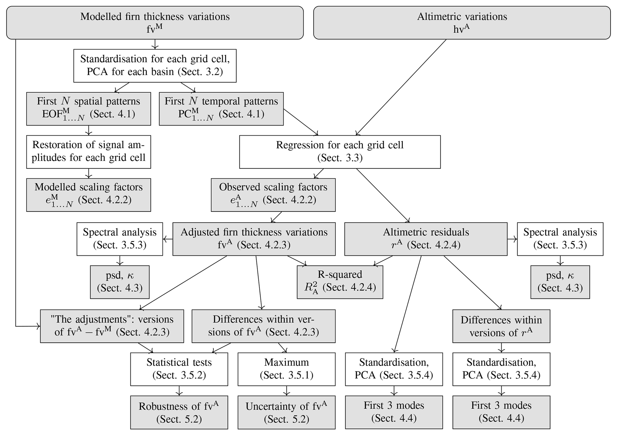
Figure 1 Workflow of the analysis. Grey boxes are the results, their notation, and the section where they are first presented. White boxes are the main methodological steps to derive these results and the sections where they are explained.

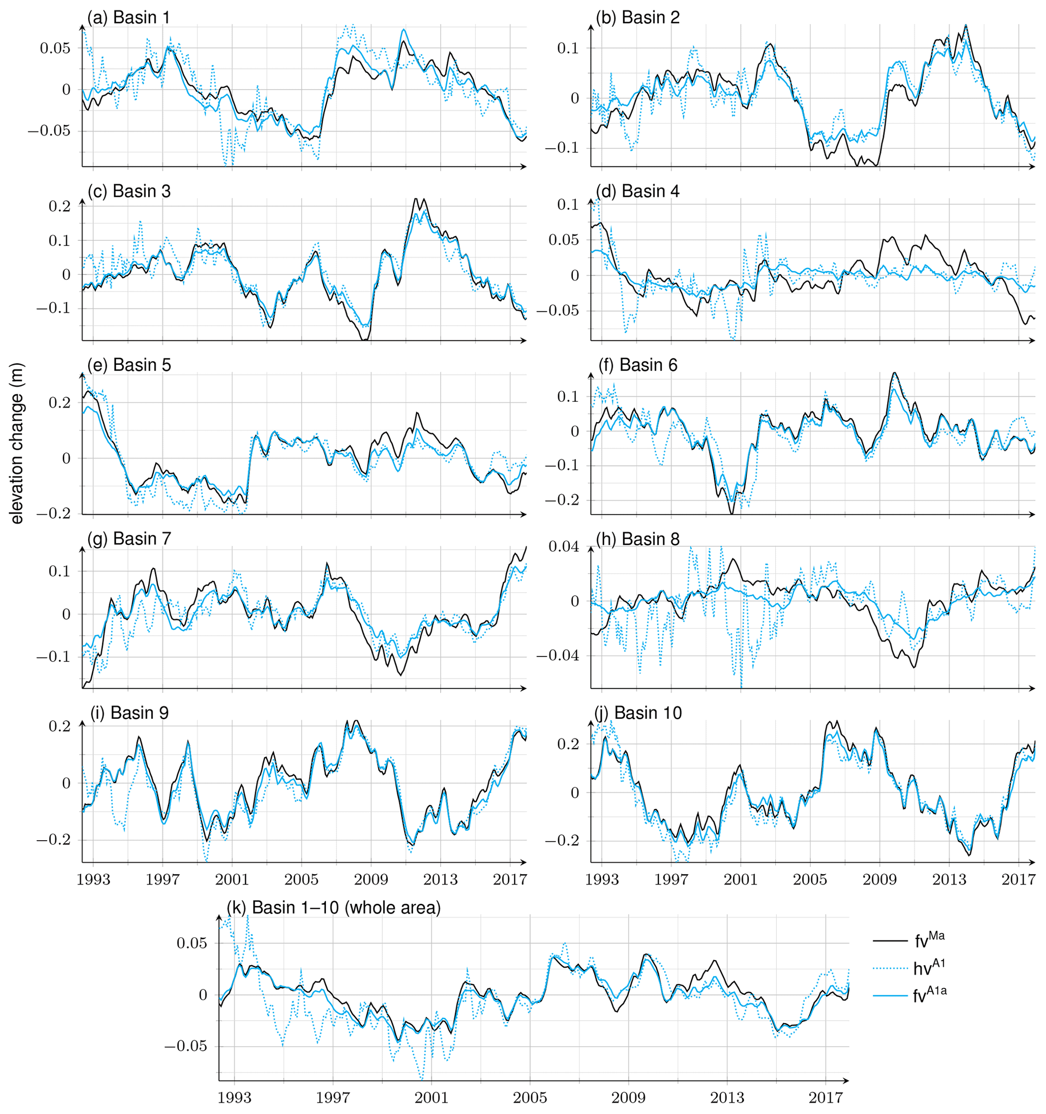
Figure 2 Basin-mean time series of modelled firn thickness variations from Veldhuijsen et al. (2023), fv^Ma (solid, black); of altimetric variations from Schröder et al. (2019a), hv^A1 (dotted, cyan); and of adjusted firn thickness variations based on A1a, fv^A1a (solid, cyan). Basin definitions are shown in Fig. 3.

3.2 Principal component analysis of modelled firn thickness variations

We identify dominant temporal patterns in firn thickness variations by principal component analysis (PCA). PCA, also called empirical orthogonal function (EOF) analysis, is applied to identify dominant modes of variability, represented by pairs of a principal component (PC) and an EOF, which represent the temporal and spatial patterns, respectively (Preisendorfer, 1988; Jolliffe, 2002; Forootan and Kusche, 2012; Boergens et al., 2014).

The PCA is performed on the modelled firn thickness variations, fv^M, after their standardisation. We standardise the time series of fv^M for each grid cell (i.e. we shift and scale it such that it has zero mean and a standard deviation (SD) of 1) because we aim to equally represent the patterns of temporal evolution regardless of location or absolute amplitudes. Otherwise, PCA results would mainly reflect patterns that are dominant at the margins, where the amplitudes of SMB and firn thickness variations are much larger than in the interior (van Wessem et al., 2018; Lenaerts et al., 2019). To regain interpretable magnitudes of the EOFs, the EOFs are multiplied by the SD of the time series of fv^M for each grid cell, which was previously used for standardisation. After this restoration of the signal amplitudes, we no longer speak of EOFs but of modelled scaling factors, e^M.

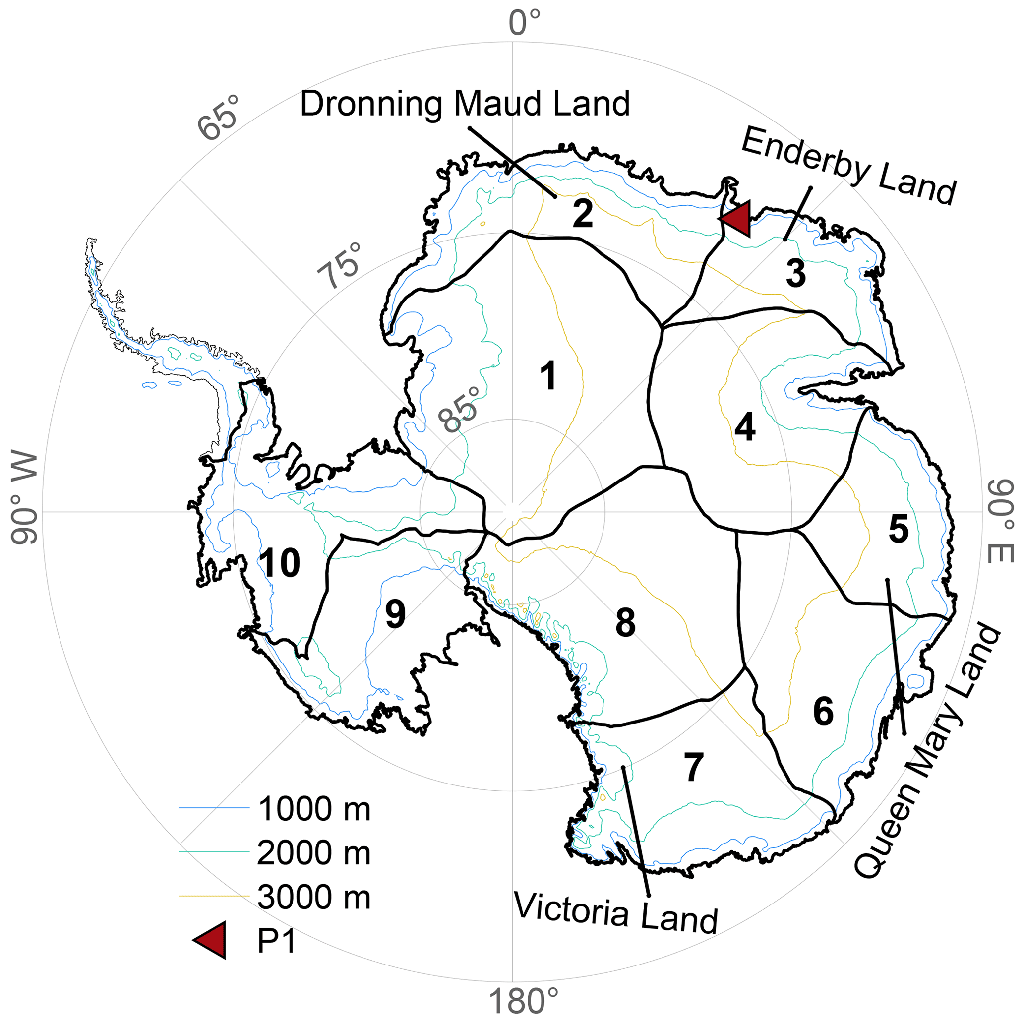
Figure 3 Drainage basins of the EAIS and WAIS used in this study (thick black lines), slightly modified from the definition of Rignot et al. (2011a, b). The outline of the Antarctic Peninsula is indicated by a thin black line. Contour lines of the ice sheet surface are shown at 1000, 2000, and 3000 m. We use the polar stereographic projection EPSG:3031 (WGS84, latitude of true scale: 71° S, central meridian: 0°). All further maps are displayed in the same projection and with the same spacing of longitude grid lines (every 45°) and latitude grid lines (every 10°).

We separately apply the PCA to fv^M for 10 basins that together cover the East Antarctic Ice Sheet (EAIS) and the WAIS (Fig. 3). To define the basins, we make use of the drainage basin definition by Rignot et al. (2011a, b) and aggregate neighbouring basins smaller than ∼600 000 km². The decision which of the original 15 basins are aggregated is guided by the correlations between the first three PCs of a preliminary PCA per original basin. For each of the 10 basins, we choose the first N modes that explain at least 90 % of the total variance of the (standardised) data. In addition, North's rule of thumb (North et al., 1982) is applied to test whether the eigenvalues of these N patterns are well separated with respect to their errors. The first N dominant temporal patterns, ${\mathrm{PC}}_{\mathrm{1}\mathrm{\dots }N}^{\mathrm{M}}$, enter the regression approach in a normalised form.

3.3 Regression approach

For each 10 km × 10 km grid cell, we describe the time series of monthly altimetric variations, hv^A, by

$$\begin{array}{}\text{(1)}& {\displaystyle }{\mathrm{hv}}^{\mathrm{A}}\left(t\right)=a+\sum _{n=\mathrm{1}}^N{e}_n^{\mathrm{A}}{\mathrm{PC}}_n^{\mathrm{M}}\left(t\right)+r^{\mathrm{A}}\left(t\right).\end{array}$$

The scaling factors, $e_{\mathrm{1}\mathrm{\dots }N}^{\mathrm{A}}$, and the offset, a, are estimated by a least-squares adjustment. The dominant temporal patterns in modelled firn thickness variations, ${\mathrm{PC}}_n^{\mathrm{M}}\left(t\right)$, refer to the basin to which the grid cell belongs. The residuals of the fit are r^A.

We define a combined product by the linear combination of Eq. (1), evaluated per grid cell and time:

$$\begin{array}{}\text{(2)}& {\displaystyle }{\mathrm{fv}}^{\mathrm{A}}\left(t\right)=\sum _{n=\mathrm{1}}^N{e}_n^{\mathrm{A}}{\mathrm{PC}}_n^{\mathrm{M}}\left(t\right).\end{array}$$

We refer to fv^A(t) as the “adjusted firn thickness variations”.

We use different weights for the observations from different time periods. As results from the older altimetry missions generally have a higher noise level (Schröder et al., 2019a; Nilsson et al., 2022), hv^A values after 2003 are weighted by 1, while hv^A values before 2003 are given a different (usually lower) weight, which is defined, individually for every grid point, by the ratio of the noise variance of hv^A before and after 2003. We assess the noise by the high-pass filtered version of hv^A separately for both periods (cf. Groh et al., 2019). The high-pass filtering consists of removing a low-pass filtered version of hv^A, where the low-pass filter is a Gaussian filter with a filter width of 6σ=12 months.

To assess the goodness of fit, we calculate the values of R squared, R², as

$$\begin{array}{}\text{(3)}& {\displaystyle }{R}_{\mathrm{A}}^{\mathrm{2}}{\displaystyle }=\mathrm{1}-{\displaystyle \frac{\mathrm{SS}\left(r^{\mathrm{A}}\right)}{\mathrm{SS}\left({\mathrm{hv}}^{\mathrm{A}}\right)}}=\mathrm{1}-{\displaystyle \frac{\mathrm{SS}\left(r^{\mathrm{A}}\right)}{\mathrm{SS}({\mathrm{fv}}^{\mathrm{A}}+r^{\mathrm{A}})}},\end{array}$$

where SS(r^A) and SS(hv^A) are the residual and total sum of squares, respectively. $\mathrm{SS}\left(r^{\mathrm{A}}\right)/\mathrm{SS}\left({\mathrm{hv}}^{\mathrm{A}}\right)$ describes the proportion of unexplained variance. We calculate R² for every grid cell individually.

3.4 Different versions of adjusted firn thickness variations

We derive two different sets of PC^M, depending on the firn model incorporated. Our annotation distinguishes the firn models by superscripts “Ma” and “Mb” for the model by Veldhuijsen et al. (2023) and Medley et al. (2022a), respectively. The regression approach (Eq. 1) is applied with each set of PC^M and equally to each of the two products of hv^A from Schröder et al. (2019a) and Nilsson et al. (2022), which we distinguish by superscripts “A1” and “A2”, respectively. All combinations of data sets used result in four applications of the regression approach (Table 1). Thus, we obtain four versions of adjusted firn thickness variations (fv^A1a, fv^A2a, fv^A1b, fv^A2b), altimetric residuals (r^A1a, r^A2a, r^A1b, r^A2b), and R squared ($R_{\mathrm{A}\mathrm{1}\mathrm{a}}^{\mathrm{2}}$, $R_{\mathrm{A}\mathrm{2}\mathrm{a}}^{\mathrm{2}}$, $R_{\mathrm{A}\mathrm{1}\mathrm{b}}^{\mathrm{2}}$, $R_{\mathrm{A}\mathrm{2}\mathrm{b}}^{\mathrm{2}}$).

(Schröder et al., 2019a)(Veldhuijsen et al., 2023)(Nilsson et al., 2022)(Veldhuijsen et al., 2023)(Schröder et al., 2019a)(Medley et al., 2022a)(Nilsson et al., 2022)(Medley et al., 2022a)

Table 1 Names of the four different versions of regression results derived by applying the regression approach of Eq. (1) with different data sets.

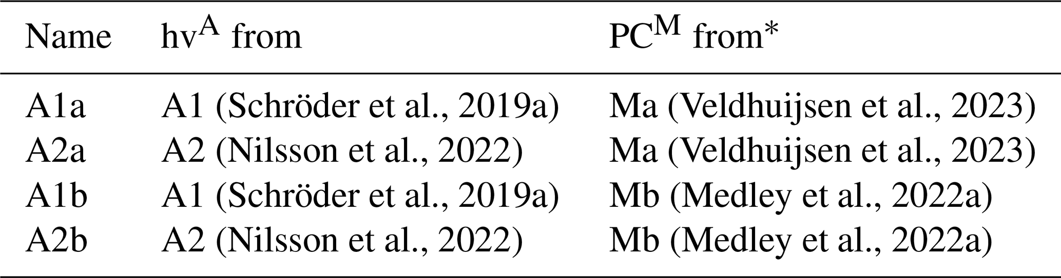
^* Standardised fv^M (Sect. 3.2).

In Appendix A1, we additionally assess three alternative ways of defining “adjusted” firn thickness variations. These alternatives are the following. (E1) Accept the modelled firn thickness variations, fv^M, without any adjustment to altimetry. (E2) Instead of using PCA-based dominant temporal patterns, use the modelled time series of firn thickness variations at every grid cell and scale it to fit the altimetry. We refer to the results as scaled firn thickness variations, fv^E2. (E3) Omit the standardisation step prior to the PCA and proceed according to Eqs. (1) and (2). We refer to the result as modified adjusted firn thickness variations, fv^E3. Note that we do not introduce fv^E1 as this would correspond to fv^M.

3.5 Assessment methods

3.5.1 Uncertainty in adjusted firn thickness variations

We assess the impact of the choice of data sets and thus the influence of different errors in the adjusted firn thickness variations, fv^A, using differences between the time series of the various versions of firn thickness variations. For each time series of differences we can calculate the temporal root mean square (rms). This is done for time series per grid cell and also for time series of basin averages. To assess the uncertainty in fv^A we consider the maximum deviation within the different versions of fv^A (Table 1). For this purpose, we form the six possible differences from fv^A1a, fv^A2a, fv^A1b, and fv^A2b and take the maximum of the rms differences.

3.5.2 Robustness of adjusted firn thickness variations

We refer to the differences between adjusted and modelled firn thickness variations as “the adjustments” (fv^A−fv^M). We consider these adjustments to be improvements over the firn models if the differences within different versions of fv^A are significantly smaller than the adjustments. We test for significance by comparing the distributions of their temporal rms. We use a two-sample, one-sided Kolmogorov–Smirnov test which is a non-parametric hypothesis test as the differences in fv do not follow a normal distribution. The Kolmogorov–Smirnov test uses the empirical cumulative distribution function to compare the distributions of two samples (Massey, 1951; Miller, 1956; Marsaglia et al., 2003). The null hypothesis (H0) reads as follows: both samples, the data of both differences to be compared, are from the same continuous distribution. Thus, the alternative hypothesis (H1) reads as follows: the empirical cumulative distribution function of sample 1 (the differences within fv^A) is larger than the empirical cumulative distribution function of sample 2 (the adjustments); that is, the differences within fv^A tend to be smaller than the differences between fv^A and fv^M.

3.5.3 Spectral analysis of regression results

We analyse the time series of altimetric residuals, r^A, and adjusted firn thickness variations, fv^A, in the spectral domain through their power spectral density (PSD) and their spectral indices, κ (Bos et al., 2012). As r^A and fv^A do not yield a white noise behaviour, we use the formulation of power-law noise to approximate their stochastic properties. For example, a power law with $\mathit{\kappa }=-\mathrm{1}$ and $\mathit{\kappa }=-\mathrm{2}$ represents flicker and random-walk noise, respectively.

3.5.4 Principal component analysis of altimetric residuals

The altimetric residuals, r^A, are further analysed in the spatio-temporal domain. First, we perform PCA on the altimetric residuals themselves to further identify dominant signals related to ice sheet processes not considered or incorrectly represented by the firn models. Note that the residuals may additionally contain signals related to variations in ice flow dynamics or subglacial hydrology. Second, we perform PCA on the residual differences to further detect and investigate prevailing uncertainties in the altimetry analysis. Only data after 2003 are used because of the higher noise level in the altimetry measurements of the older satellite missions. Test experiments showed that errors in pre-2003 data bias the dominant modes, hardly helping to distinguish between signal and error. We standardise the time series of residuals and residual differences, as we did previously when identifying dominant patterns in modelled firn thickness variations (Sect. 3.2).

The first PCA is applied to the four versions of standardised residuals (r^A1a, r^A1b, r^A2a, r^A2b). The second PCA is applied to the two versions of standardised residual differences (r^A1a−r^A2a and r^A1b−r^A2b). Since we are interested in the common characteristics of the four residual data sets on the one hand and the two difference data sets on the other, we combine the individual data sets and concatenate them to form a “super data matrix”. Specifically, our data sets comprise m=90 638 points in space (entire area under investigation) and p=108 points in time (2003–2017). Thus, the first and second PCA is applied to the super data matrix of the size 4m×p and 2m×p, respectively. The PCA is conducted to identify the dominant temporal patterns (PCs), which are shared by all versions, together with their space-dependent and version-dependent spatial patterns (EOFs). Each identified mode thus consists of one joint PC (1×p) and four or two EOFs (4m×1 or 2m×1) in the case of the first or second PCA, respectively.

4 Results

4.1 Dominant patterns in modelled firn thickness variations

We can explain at least 90 % of the total variance of the modelled firn thickness variations, fv^Ma, with two modes (basin 5), three modes (basins 1, 3, and 6), four modes (basins 2, 4, and 8), and five modes (basins 7, 9, and 10). The modes (i.e. the PC–EOF pairs) reveal a typical hierarchy of an autocorrelated geophysical signal, as shown in Fig. 4 for the region of Dronning Maud Land (basin 3). The first EOF is almost uniform over the entire basin (Fig. 4a). The spatial features of the second EOF follow the topography from north to south (Fig. 4b), and the third EOF exhibits an east–west gradient (Fig. 4c). The first PC shows a lower-frequency signal than the following PCs. All three PCs fluctuate over time similar to an integrated random-walk process (Fig. 4d). In the case of basin 3, 74 % of the variance is explained by the first mode, which captures the accumulation events in 2009 and 2011 (Boening et al., 2012; Lenaerts et al., 2013) as shown by the characteristic increase in the PC during these years (Fig. 4d). All subsequent modes are more difficult to interpret as a geophysical signal because their determination is governed by the mathematical orthogonality property of PCs.

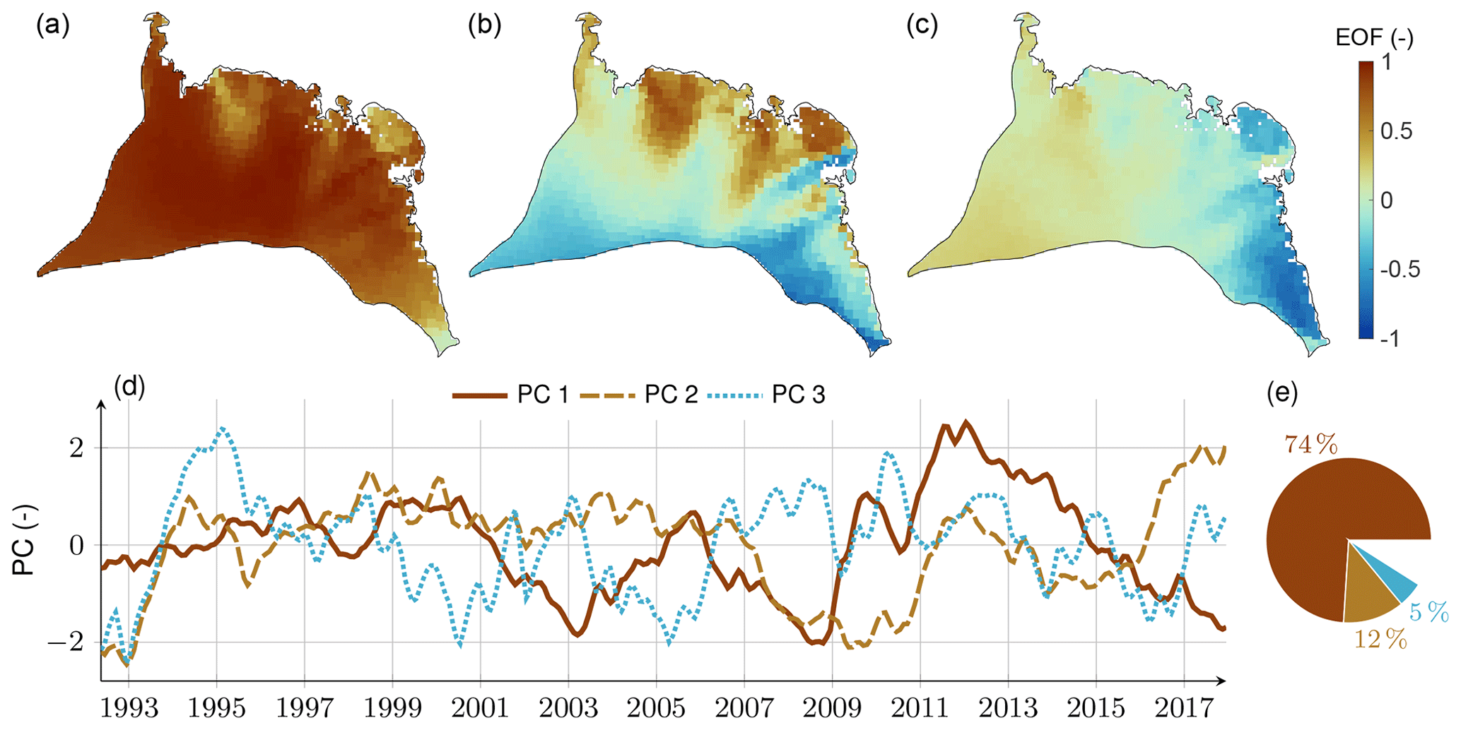
Figure 4 PCA results of basin 3: dominant patterns in firn thickness variations identified from standardised firn modelling data (Ma). (a–c) First three spatial patterns (EOFs). (d) First three temporal patterns (PCs). (e) Associated percentages of the basin's total data variance. Results for all basins and for both firn models, Ma and Mb, are given by Figs. S5–S9.

4.2 Regression results

4.2.1 Time series for a selected grid point

Figure 5 exemplifies the derivation of adjusted firn thickness variations for a selected grid point, P1, and based on the regression A1a (Table 1). P1 (37.7° E, 70.2° S) is located in basin 3 close to the ice sheet margin at ∼1080 m height (Fig. 3). There, the adjusted and modelled firn thickness variations, fv^A1a and fv^Ma, have an SD of 40.5 and 51.5 cm, respectively (Fig. 5a). By construction, the scaling factors, e_1…3, equal the SD of the associated scaled dominant temporal patterns. In the presence of data gaps in the altimetry time series, this equality approximately holds. Both fv^A1a and fv^Ma are dominated by ${\mathrm{PC}}_{\mathrm{1}}^{\mathrm{Ma}}$ (Fig. 5b), as this pattern is scaled by $e_{\mathrm{1}}^{\mathrm{A}\mathrm{1}\mathrm{a}}=\mathrm{39.2}$ cm (altimetry) and $e_{\mathrm{1}}^{\mathrm{Ma}}=\mathrm{48.4}$ cm (firn model). The second pattern, ${\mathrm{PC}}_{\mathrm{2}}^{\mathrm{Ma}}$ (Fig. 5c), is very small in the firn model ($e_{\mathrm{2}}^{\mathrm{Ma}}=$ +0.2 cm), while it is somewhat larger and has an opposite sign for altimetry ($e_{\mathrm{2}}^{\mathrm{A}\mathrm{1}\mathrm{a}}=-\mathrm{7.7}$ cm) but is still small enough to contribute little to fv^A1a.

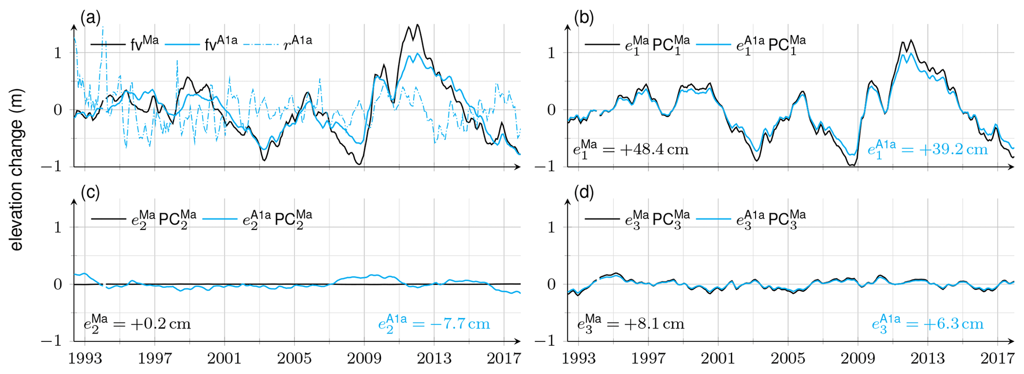
Figure 5 Regression results for the grid point P1 (Fig. 3). (a) Modelled firn thickness variations, fv^Ma (solid, black); adjusted firn thickness variations, fv^A1a (solid, cyan); and altimetric residuals, r^A1a (dash-dotted, cyan). (b–d) Scaled first, second, and third PC^M from the regression version A1a (cyan) and the model Ma (black). The solid cyan curve in (a) is the sum of the cyan curves in (b)–(d). Time series of a larger subset of selected grid points (Fig. S10) are shown in Figs. S11 and S12.

The SD of altimetric residuals, r^A1a, is 31.7 cm, less than the SD of fv^A1a (Fig. 5a). The R-squared value of $R_{\mathrm{A}\mathrm{1}\mathrm{a}}^{\mathrm{2}}$ (Eq. 3) is 0.601. When calculated separately for the time before and after 2003, $R_{\mathrm{A}\mathrm{1}\mathrm{a}}^{\mathrm{2}}$ equals −0.004 and 0.831, respectively. Thus, the adjusted firn thickness variations, fv^A1a, describe less of the altimetry variance before 2003, while after 2003 they explain 83 %. Because of the different weighting of hv^A before and after 2003 (Sect. 3.3), $R_{\mathrm{A}}^{\mathrm{2}}$ can indeed be negative and distinguishing the two periods is reasonable.

4.2.2 Scaling factors, e

The scaling factors, $e_{\mathrm{1}\mathrm{\dots }\mathrm{3}}^{\mathrm{A}\mathrm{1}\mathrm{a}}$ and $e_{\mathrm{1}\mathrm{\dots }\mathrm{3}}^{\mathrm{Ma}}$, per grid cell are mapped for the example of basin 3 in Fig. 6. The patterns of the factors, like the EOFs (Fig. 4), follow a typical hierarchy discussed in Sect. 4.1. Overall, the patterns of $e_{\mathrm{1}\mathrm{\dots }\mathrm{3}}^{\mathrm{Ma}}$ agree for a large part with $e_{\mathrm{1}\mathrm{\dots }\mathrm{3}}^{\mathrm{A}\mathrm{1}\mathrm{a}}$. However, the first spatial pattern from the model extends further into the ice sheet interior than the pattern from altimetry (Fig. 6d versus a). In general, scaling factors from the model show a smoother and more blurred pattern than the ones adjusted to altimetry. Patterns from altimetry reveal a higher level of detail and a more localised spatial distribution. At certain regions the spatial distributions also differ, e.g. for the second pattern in the vicinity of P1 (Fig. 6b versus e). The spatial variation in the scaling factors along two selected profiles is given in Fig. S13, and a comprehensive representation of the scaling factors for all basins with the different choices of input data is given by Figs. S5 and S14.

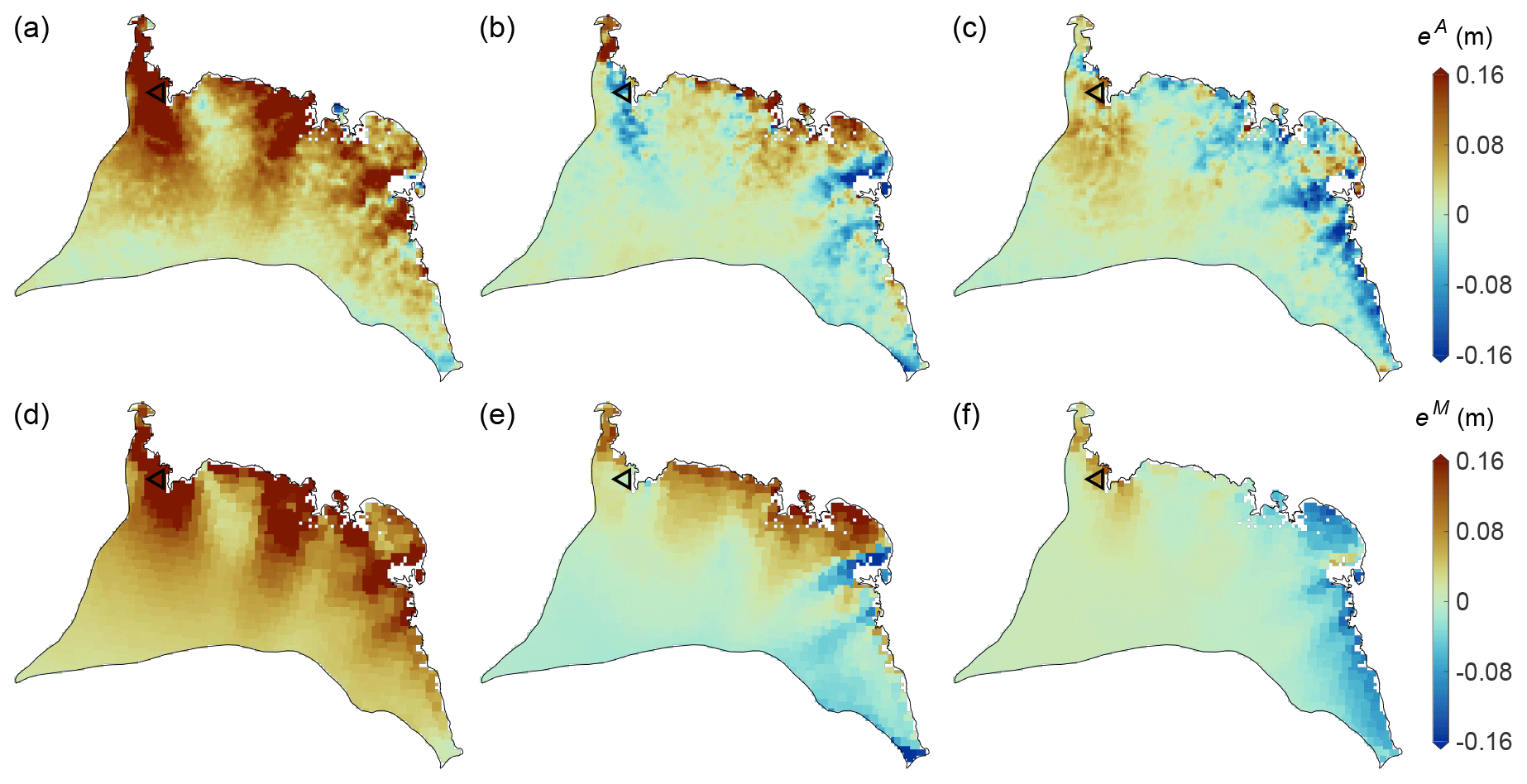
Figure 6 Scaling factors for basin 3. (a–c) $e_{\mathrm{1}\mathrm{\dots }\mathrm{3}}^{\mathrm{A}\mathrm{1}\mathrm{a}}$ is the first three observed factors from the regression A1a. (d–f) $e_{\mathrm{1}\mathrm{\dots }\mathrm{3}}^{\mathrm{Ma}}$ is the first three modelled factors from Ma. Panels (d)–(f) are the same as Fig. 4a–c but with restored signal amplitudes for each grid cell. The location of P1 is shown by the black triangle.

4.2.3 Firn thickness variations and their sensitivity to the choice of data sets

In general, the spatial patterns of the rms of the adjusted firn thickness variations, fv^A, and the modelled firn thickness variations, fv^M, are similar (Fig. 7a and b). The rms values are largest at the ice sheet margin and smallest over the plateau of the EAIS. For grid cells in the elevation ranges of (1) below 1000 m, (2) 1000 to 2000 m, (3) 2000 to 3000 m, and (4) above 3000 m, median rms values are in the range of (1) 12.2 to 16.4 cm, (2) 8.3 to 10.9 cm, (3) 3.5 to 5.1 cm, and (4) 2.1 to 2.3 cm, respectively. Differences between adjusted and modelled variations reveal the highest absolute rms values at lower elevations, near the AIS margins with median rms differences in the range of 13.4 to 14.7 cm below 1000 m (Fig. 7c). In a relative sense, the largest mismatch is found not only in the interior of the EAIS but also at some locations on the ice sheet margin (Fig. 7d).

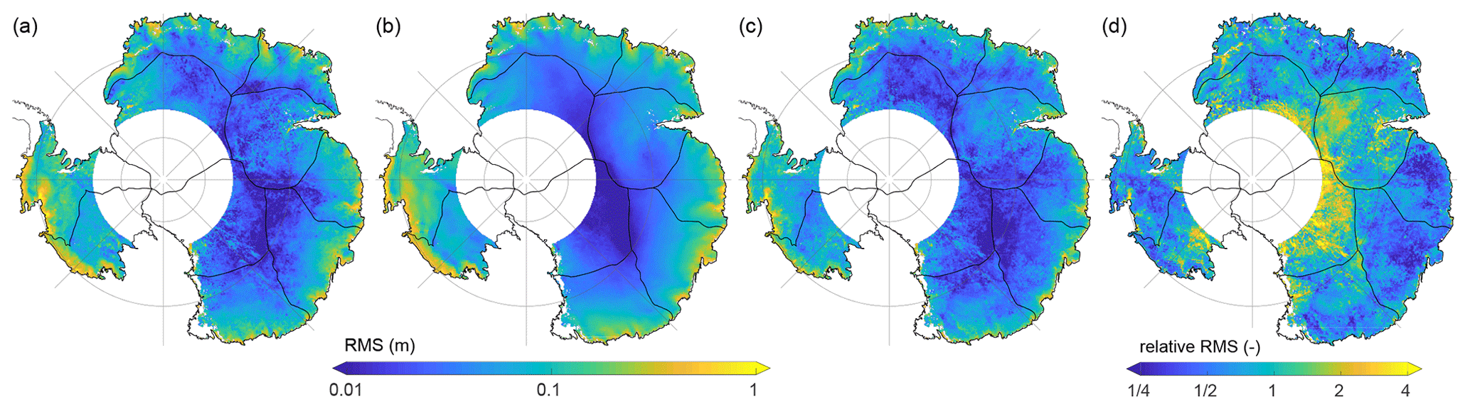
Figure 7 Root mean square (rms) of the times series of (a) adjusted firn thickness variations based on A1a, fv^A1a, and (b) modelled firn thickness variations based on Ma, fv^Ma. (c) The rms of the time series of the differences of fv^A1a−fv^Ma. (d) The rms of the time series of the differences of fv^A1a−fv^Ma divided by the rms of fv^Ma. All versions of fv^A and fv^M are illustrated in Figs. S15 and S16.

To evaluate the sensitivity of fv to the choice of data sets, we calculate the difference between various versions of fv (Sect. 3.5.1) and compare the distributions of the rms of these differences (Fig. 8). In total, differences within fv^A are smallest, followed by differences within fv^M, while differences between fv^A and fv^M are largest (Fig. 8, Table 2). Differences within fv^A indicate a smaller influence by different firn model data than by different altimetry data. Differences between fv^A and fv^M are smallest for A1a (adjustment over the firn model Ma through altimetry A1), largest for A2b (adjustment over the firn model Mb through altimetry A2) in a relative sense, and largest for A1b (adjustment over the firn model Mb through altimetry A1) in an absolute sense (Table 2).

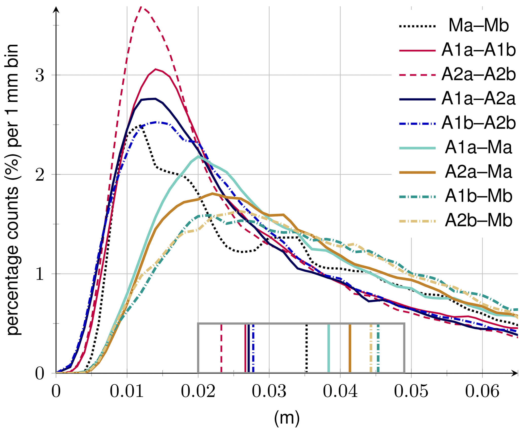
Figure 8 Histograms of the temporal rms, assessed at each grid cell, of differences between various versions of firn thickness variations. Vertical lines in the box indicate median values. Corresponding rms maps of differences are displayed in Figs. S15–S17.

Table 2 Overview of the comparison between various versions of firn thickness variations, as detailed in Fig. 8. Column 1 indicates the addressed comparison: between versions of adjusted firn thickness variations, fv^A (rows 1–4); between modelled firn thickness variations, fv^M (row 5); and between fv^A and fv^M (rows 6–9). For each comparison, column 2 gives the median (over all grid cells) of the rms (over time) of differences between the two time series evaluated at each grid cell. The table is ordered by the median values (from small to large). Column 3 also gives the median of the rms of differences but as a relative measure. For each grid cell, the rms of differences are divided by the rms of fv^Ma. Then, the median over all grid cells is calculated. Column 4 gives a short description or possible causes.

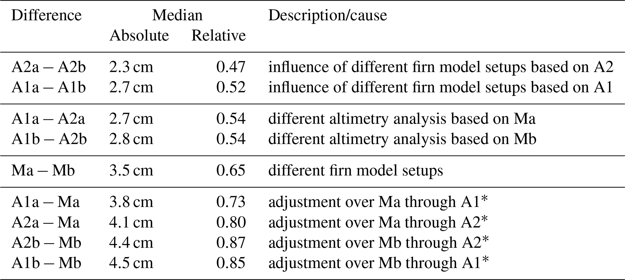
^* Due to firn signals not being correctly represented by the models (firn model errors) and/or due to errors in the altimetry products.

The differences between the various versions of fv reflect errors in the firn models and in the altimetry products. These are further discussed in Sect. 5.3 and 5.4.

4.2.4 Goodness of fit

The altimetric residuals are used to calculate the goodness of fit or R² (Eq. 3). The rms of the altimetric residual time series and the values of R squared based on the regression A1a, $R_{\mathrm{A}\mathrm{1}\mathrm{a}}^{\mathrm{2}}$, are presented in Fig. 9a and b, respectively, for the period after 2003. The rms of the residuals after 2003 is generally smaller than before 2003 (Fig. S18) due to the different noise levels and weighting of the altimetry observations in the two periods (Sect. 3.3) so that R² is generally higher after 2003 than before 2003 (Fig. S19).

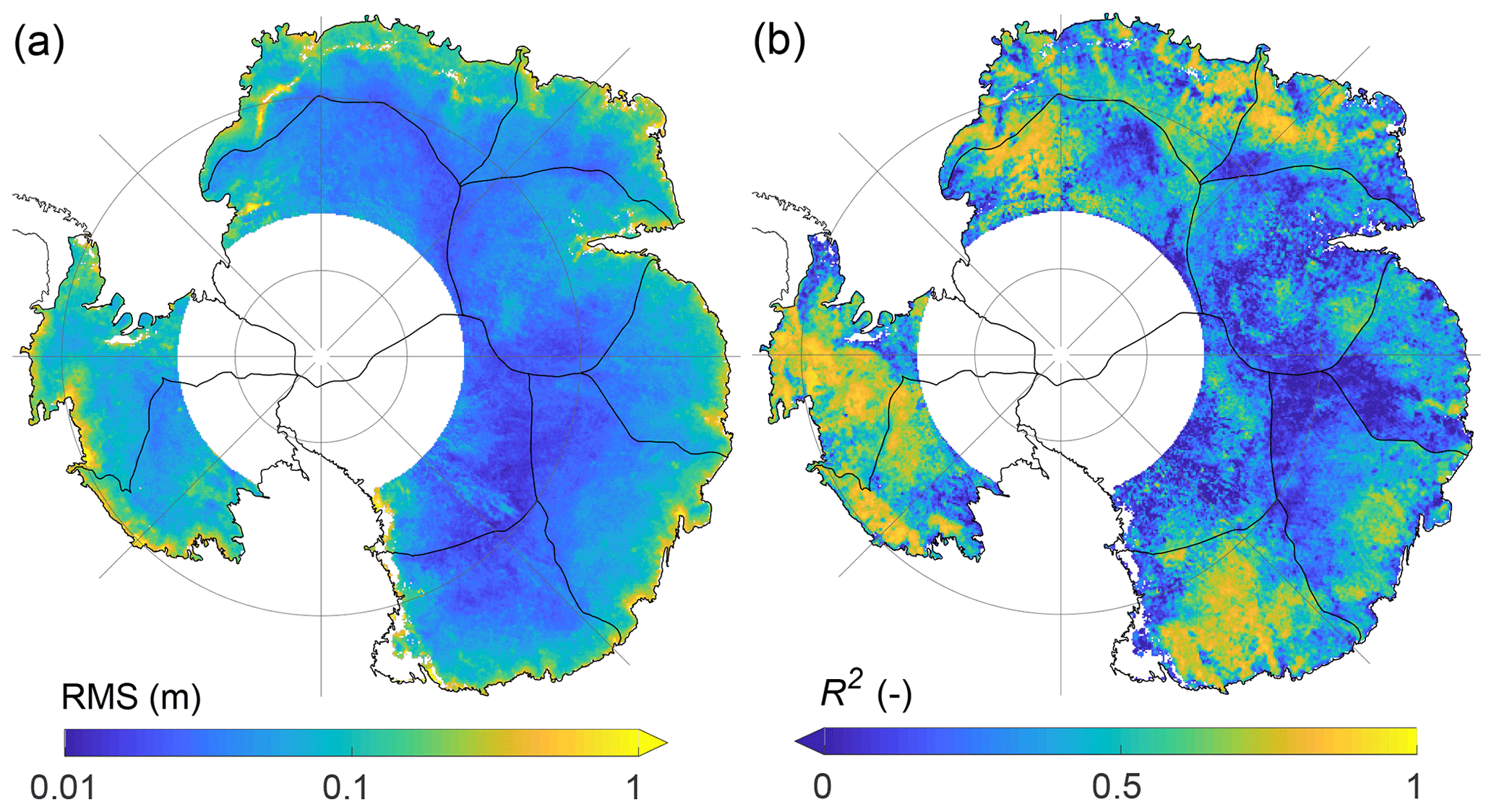
Figure 9 (a) The rms of the residual altimetric time series, r^A1a, for the period after 2003. (b) Values of R squared for the regression A1a, $R_{\mathrm{A}\mathrm{1}\mathrm{a}}^{\mathrm{2}}$, considering the period after 2003. Colour bar arrows indicate that the value range exceeds the limits of the colour scale.

After the individual calculation of R² for each grid cell, basin-mean values are derived and listed in Table 3 for all versions of regression. Averaged over the entire area, $R_{\mathrm{A}\mathrm{1}\mathrm{a}}^{\mathrm{2}}$ is 0.40 after 2003 (Table 3). This means that on average 40 % of the variance of altimetric variations is captured by the regression model, i.e. by fv^A1a. Depending on the basin, fv^A1a captures 26 % (basins 4 and 8) to 58 % (basin 10) of the data variance. In general, we find less agreement with altimetry when incorporating the Mb firn model instead of the Ma firn model (Table 3, column A1a versus A1b and column A2a versus A2b).

Table 3 Explained variance or R squared, R², for each basin and each version of regression (Table 1) over the period after 2003. Apart from the last column ($\stackrel{\mathrm{‾}}{\mathrm{A}\mathrm{1}\mathrm{a}}$), R² is first calculated for each grid cell according to Eq. (3) and then averaged over each basin. Values of $\stackrel{\mathrm{‾}}{\mathrm{A}\mathrm{1}\mathrm{a}}$ are calculated by first averaging the regression results over each basin and then applying Eq. (3). Basin averages of R² for the period before 2003 are listed in Table S1 in the Supplement.

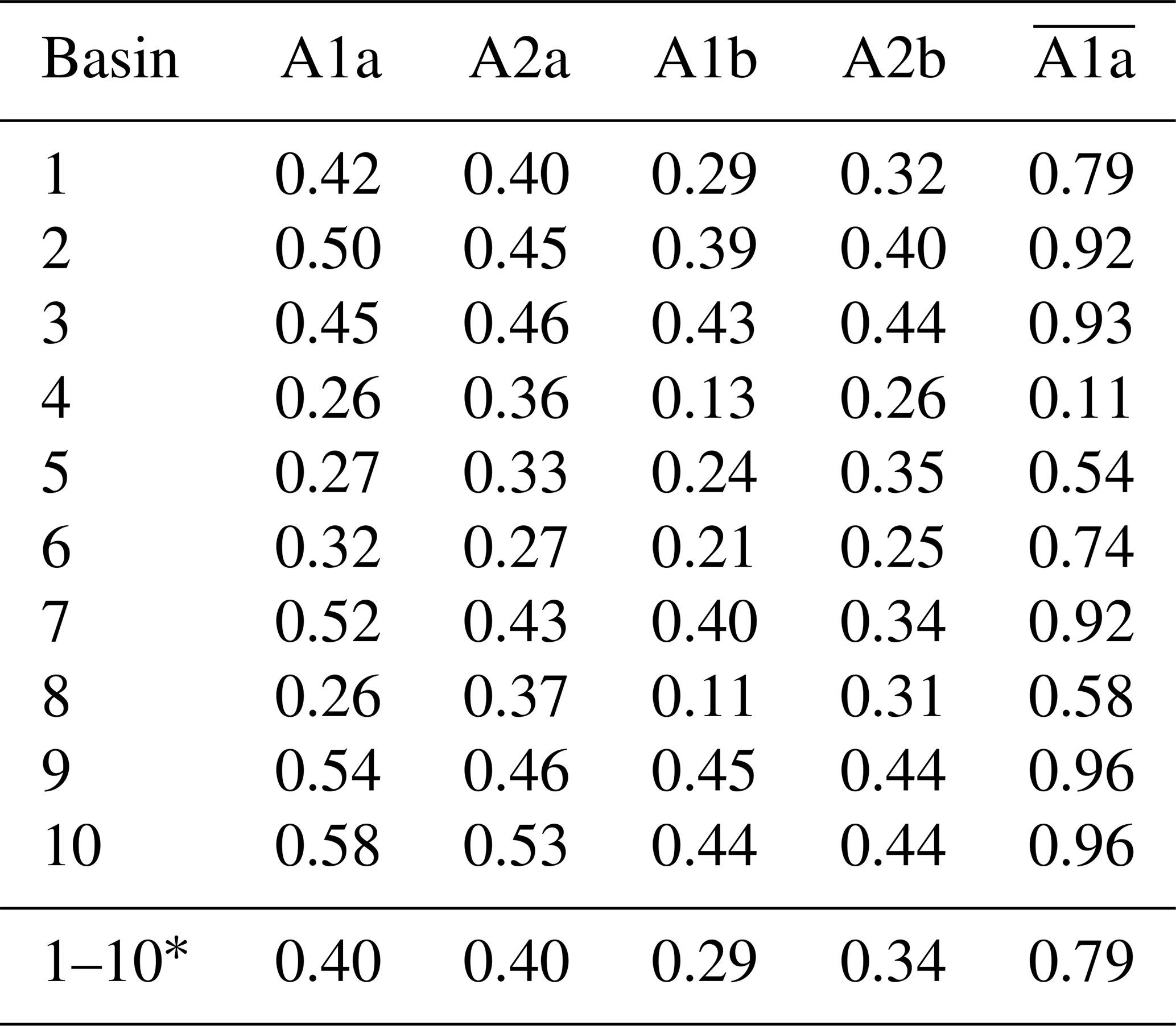
^* Refers to the entire area (considered a single basin).

The impact of methodological changes to the regression approach (E1, E2, and E3 as summarised in Sect. 3.4) is elaborated in Appendix A2. The methodological changes result in smaller average R² values (Fig. A1, Table A1), so less of the data variance can be explained. For this reason, the modified approaches are not preferable to the chosen regression approach presented in Sect. 3.3.

So far, the presented R² values are based on calculations per grid cell in accordance with the regression approach Eq. (1). For basin-average time series, R² becomes larger. Figure 2 shows the basin averages of adjusted firn thickness variations, which we may compare to the basin averages of the altimetric variations through the values of R squared given in the last column of Table 3. Indeed, fv^A1a captures up to 96 % (basins 9 and 10; WAIS) of the variance of basin-average altimetry variations. Basin-mean time series of all regression results and versions are presented in Figs. S20 and S21.

However, on the level of individual grid cells the altimetric residuals, r^A, still contain a large proportion of the variance of altimetric variations. For example, for A1a and the period after 2003, an average ratio of 60 % of the altimetric variations is unexplained. Therefore, the residuals, r^A, are further investigated in Sect. 4.3 and 4.4.

4.3 Spectral analysis of regression results

We find a stronger autocorrelation for the time series of fv^A1a than for that of r^A1a; i.e. r^A1a is closer to white noise behaviour than fv^A1a, since the power spectral density (PSD) for fv^A1a shows a steeper decrease with frequency than for r^A1a (Fig. 10a). At low frequencies the PSD of fv^A1a generally exceeds the PSD of r^A1a, while above a certain frequency (∼0.5 yr⁻¹ for P1) the PSD of r^A1 exceeds that of fv^A1a (Fig. 10a). The spectral indices, κ, determined for r^A1a and fv^A1a are −1.75 and −3, respectively, at P1. Over the entire area, the mean value of κ for r^A1a is −1.72 (Fig. 10b), which indicates temporally correlated residuals with characteristics close to random-walk noise. For fv^A1a, in contrast, the value of κ is −3 at each grid cell. The employed software to estimate κ (Bos et al., 2012) has −3 as its minimum output value. Hence, fv^A1a has $\mathit{\kappa }\le -\mathrm{3}$ and therefore a stronger autocorrelation than r^A1a.

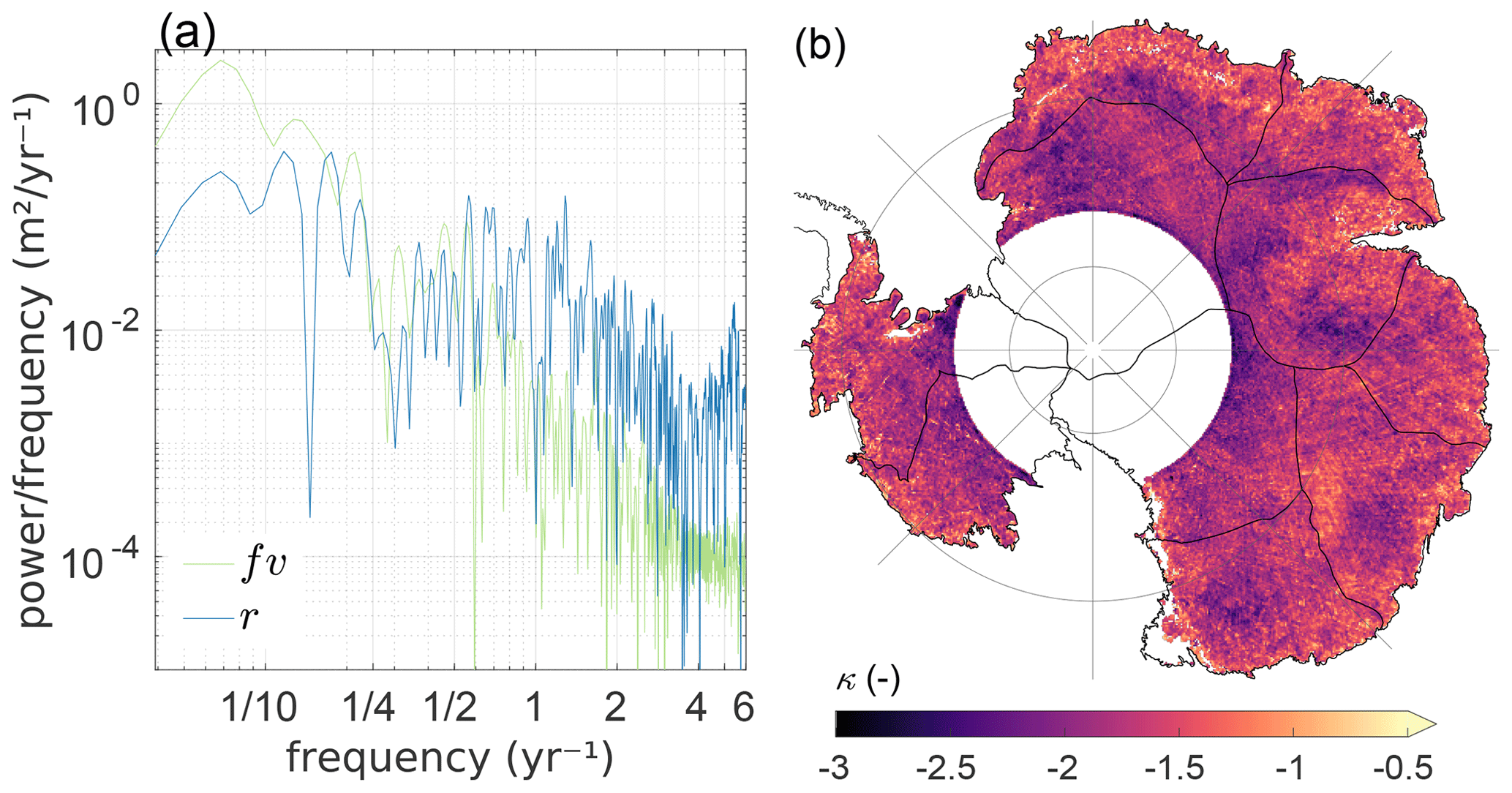
Figure 10 (a) Lomb–Scargle power spectral density (PSD) of altimetric residuals, r^A1a (blue), and adjusted firn thickness variations, fv^A1a (green), for the grid point P1. See Figs. S22 and S23 for the larger subset of selected grid points. (b) Spectral index κ for power-law noise adjusted to r^A1a of every grid cell. Colour bar arrows indicate that the value range exceeds the limits of the colour scale.

4.4 Dominant patterns in altimetric residuals

The first three dominant modes explain 23 % of the variance of altimetric residuals (Fig. 11e) and 19 % of the variance of residual differences (Fig. 12e). The first mode of the residual differences captures 10 %, and its temporal pattern reveals a prominent drop between July 2010 and January 2011 (Fig. 12d). Due to the data standardisation prior to PCA, the EOFs cannot be directly interpreted as amplitudes in elevation change. For their presentation (Figs. 11a–c and 12a–c), we restored the signal amplitudes for each grid cell by multiplying the SD of the time series, which was used beforehand to normalise the time series.

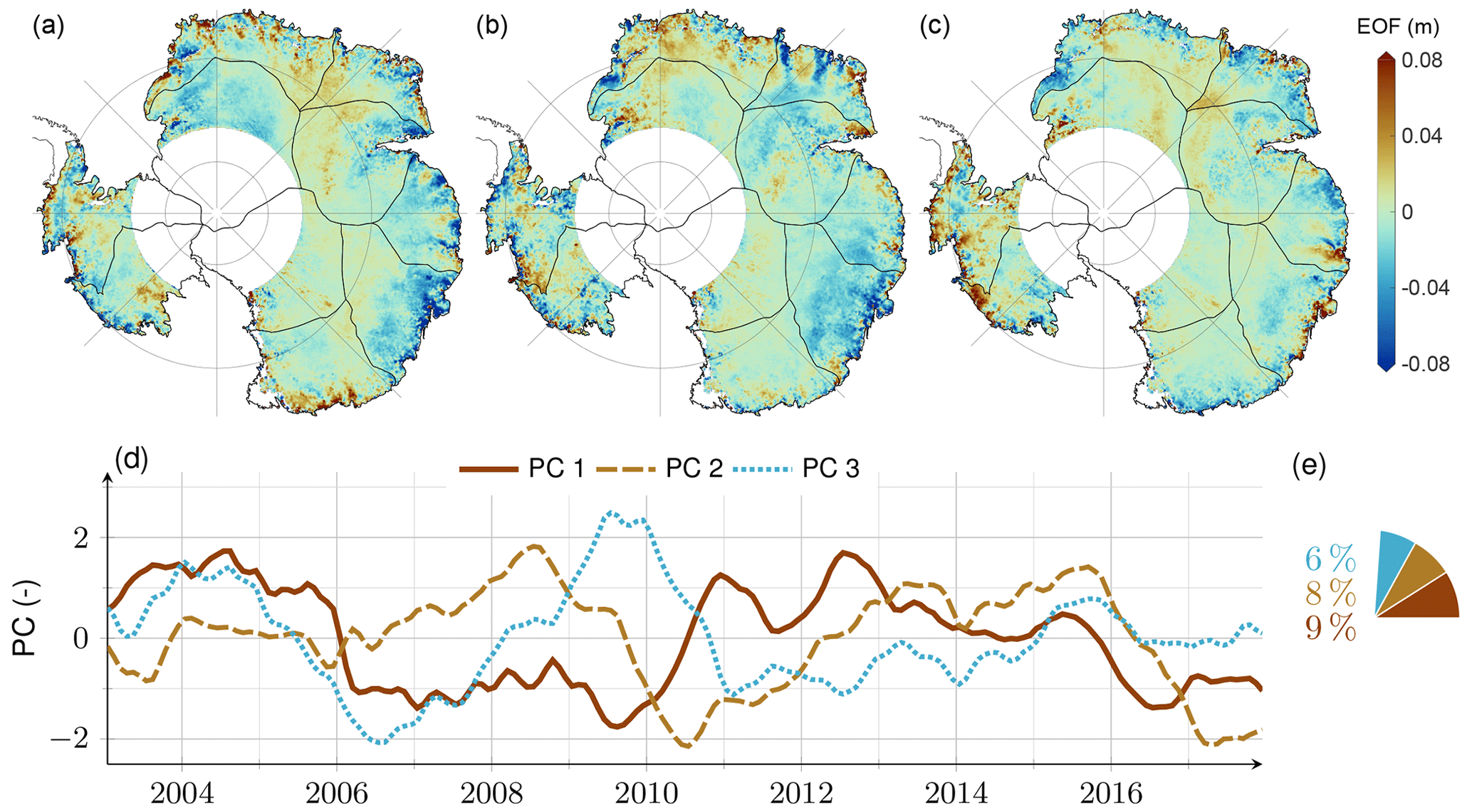
Figure 11 PCA results of standardised altimetric residuals for the period after 2003. (a–c) First three spatial patterns (EOFs) (version dependent) shown here for r^A1a and with restored signal amplitudes for each grid cell. The EOFs of all versions are illustrated in Figs. S24 and S25. (d) First three temporal patterns (PCs) determined from the aggregated data sets of r^A1a, r^A1b, r^A2a, and r^A2b. (e) Associated percentages of the total residual variance considering the respective PC–EOF pairs.

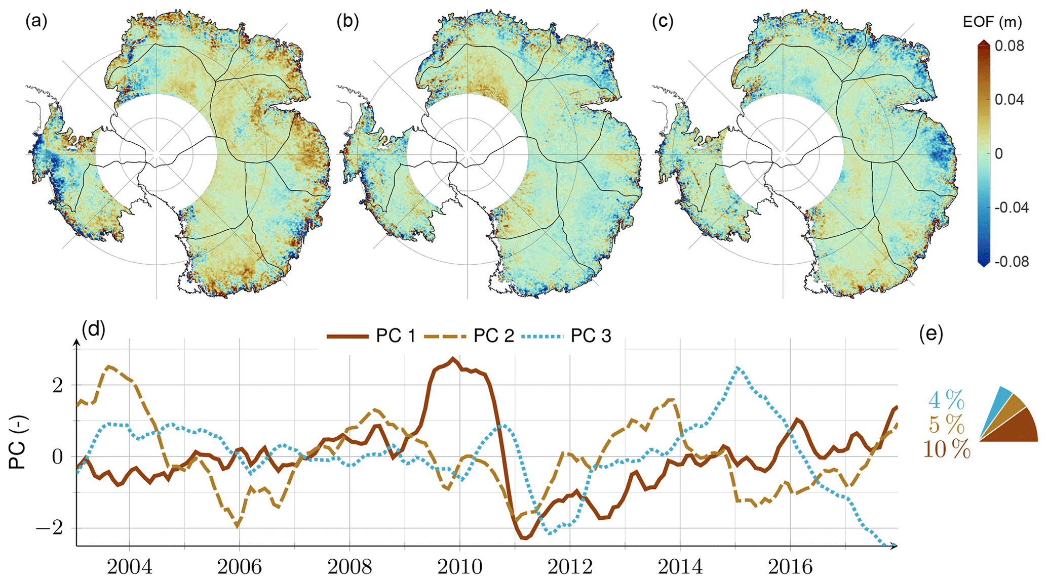
Figure 12 PCA results of standardised altimetric residual differences for the period after 2003. (a–c) First three spatial patterns (EOFs) (version dependent) shown here for r^A1a−r^A2a and with restored signal amplitudes for each grid cell. The EOFs of all versions are illustrated in Figs. S26 and S27. (d) First three temporal patterns (PCs) are the joint basis of r^A1a−r^A2a and r^A1b−r^A2b. (e) Associated percentages of the total variance of residual differences considering the respective PC–EOF pairs.

5 Discussion

5.1 Interannual firn thickness variations

In general, adjusted firn thickness variations, fv^A (e.g. Fig. 7a for version A1a), and modelled firn thickness variations, fv^M (e.g. Fig. 7b for Ma), share the same spatial patterns. The largest magnitudes are found at lower elevations near the ice sheet margins with median rms values in the range of decimetres. The smallest magnitudes are found over the plateau of the EAIS with median rms values in the range of centimetres (Sect. 4.2.3). This general spatial pattern was to be expected, as it is related to the spatial variability in SMB. Snowfall, the main driver of Antarctic SMB variability, increases from the dry, relatively flat and homogeneous interior to the steep and complex topography of the wetter coastal conditions. High snowfall at the ice sheet margins occurs due to orographic precipitation, influenced by the winds and topography of the AIS (van Wessem et al., 2014; Lenaerts et al., 2019).

The adjusted firn thickness variations, fv^A, reveal a strong temporal autocorrelation through the strong decrease in their PSD with frequency, with spectral indices $\mathit{\kappa }\le -\mathrm{3}$ for a power-law noise model (Sect. 4.3). This is in line with the findings of King and Watson (2020). They estimated the power-law noise parameter, κ, to be in the range of −2.3 to −2.2 and −3.0 to −2.6 based on SMB estimates from RACMO2.3p2 and ice core composites, respectively. Unlike our analysis, they only co-estimated a linear trend.

In the following, we compare how much variance of altimetric variations (for the period after 2003) can be explained according to the applied approach and the two different spatial considerations used previously, namely, first, the percentages assessed from grid cell time series and then averaged over the entire area, and second, the percentages from time series averaged over the entire area (“mean Antarctic” time series, Fig. 13). The modelled firn thickness variations, fv^Ma, explain 11 % and 64 % for the two spatial considerations, respectively (Table A1, columns E1 and $\stackrel{\mathrm{‾}}{\mathrm{E}\mathrm{1}}$). The scaled firn thickness variations, fv^E2, explain 31 % and 71 % (Table A1, columns E2 and $\stackrel{\mathrm{‾}}{\mathrm{E}\mathrm{2}}$), respectively. The modified adjusted firn thickness variations, fv^E3, explain 37 % and 79 % (Table A1, columns E3 and $\stackrel{\mathrm{‾}}{\mathrm{E}\mathrm{3}}$). Finally, the adjusted firn thickness variations, fv^A1a, explain 40 % and 79 % for the two spatial considerations (Table 3, columns A1a and $\stackrel{\mathrm{‾}}{\mathrm{A}\mathrm{1}\mathrm{a}}$).

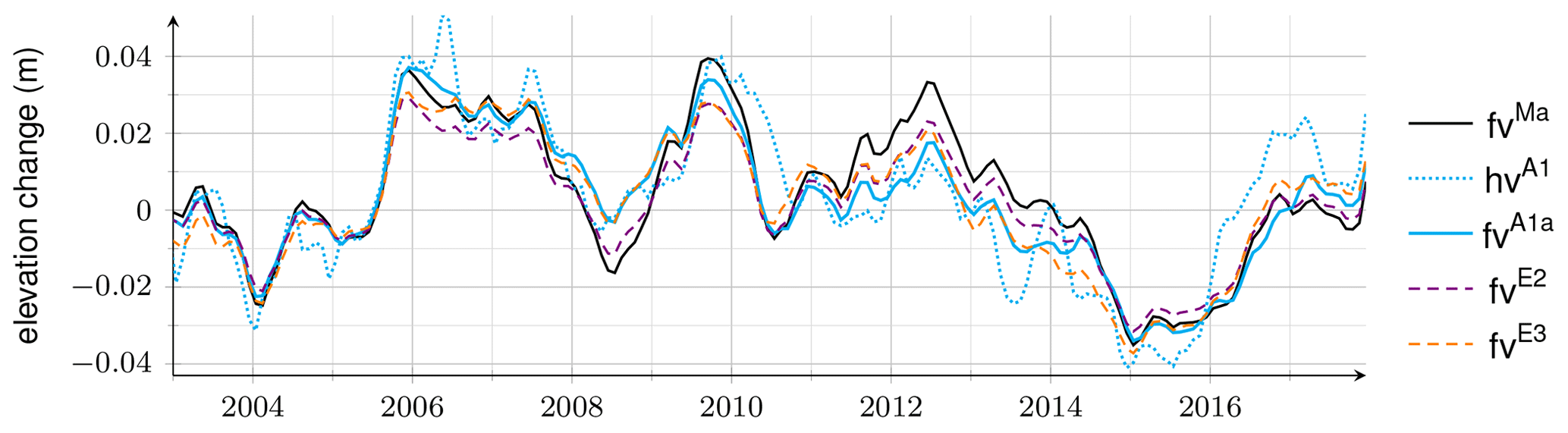
Figure 13 Mean Antarctic interannual elevation changes depending on the applied approach. Modelled firn thickness variations (fv^Ma), altimetric variations (hv^A1), adjusted firn thickness variations (fv^A1a), scaled firn thickness variations (fv^E2), and modified adjusted firn thickness variations (fv^E3).

Our regression approach (Eq. 1), which generates fv^A1a, explains a larger part of the variance of altimetric variations than the other approaches. The spatial scale investigated is crucial for the results, as the estimates from the basin-mean time series explain more of the altimetry variance than the estimates considering each grid cell equally. However, the latter are needed to understand the spatial patterns of firn variations.

5.2 Uncertainty and robustness of adjusted firn thickness variations

The adjusted firn thickness variations, fv^A, include the effects of firn model errors and altimetry errors. The differences of fv^A1a−fv^A1b (Fig. 14a) and fv^A2a−fv^A2b, evaluated at every grid cell, are used to assess the influence of different firn model setups on fv^A. The median values (over all grid cells) of absolute and relative differences are in the range of 2.3 to 2.7 cm and 47 to 52 %, respectively (Table 2, Fig. 8). The differences of fv^A1a−fv^A2a (Fig. 14b) and fv^A1b−fv^A2b, evaluated at every grid cell, are used to assess the influence of different altimetry analysis on fv^A. The median values (over all grid cells) of absolute and relative differences are in the range of 2.7 to 2.8 cm and ∼54 %, respectively (Table 2, Fig. 8). Both the firn model and altimetry errors are discussed in Sect. 5.3 and 5.4 separately.

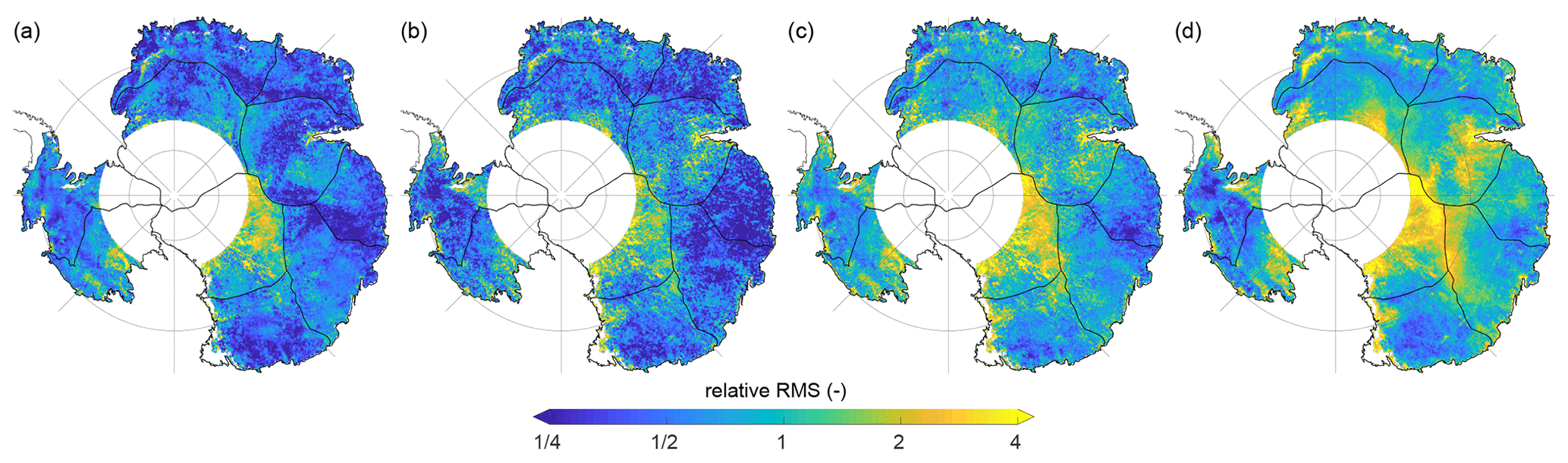
Figure 14 (a) The rms of (the time series of) the differences of fv^A1a−fv^A1b. (b) The rms of the differences of fv^A1a−fv^A2a. (c) Uncertainty estimate of fv^A: maximum rms of any combination of differences within versions of fv^A. (d) The rms of the residual differences of r^A1a−r^A2a considering only the period after 2003. All rms maps (a–d) are normalised by the rms of fv^Ma.

To assess the combined influence of firn model and altimetry errors on fv^A, the maximum deviation within the different versions of fv^A is used (Sect. 3.5.1). Figure 14c shows the map of the maximum rms values. The median values (over all grid cells) of absolute and relative (maximum) differences are ∼4.2 cm and ∼80 %, respectively. In addition, median values are calculated for every basin separately. The absolute and relative uncertainties range from 2.2 cm (basin 8) to 10.6 cm (basin 10) and from 54 % (basin 5) to 186 % (basin 8), respectively. We consider these estimates to be rough but rather conservative uncertainty assessments for the adjusted firn thickness variations. In addition to the evaluation at the grid cell level, the uncertainty in fv^A is assessed by time series differences in the basin means. See Fig. S20 for the basin-mean time series of the four versions of fv^A. The associated uncertainties per basin range from 0.9 cm (basin 4) to 6.4 cm (basin 10). The relative uncertainties are in the range of 20 % (basin 2) to 108 % (basin 8). For mean Antarctic fv^A an absolute and relative uncertainty of ∼1.3 cm and ∼66 %, respectively, are estimated.

We assess the robustness of fv^A through statistical tests according to Sect. 3.5.2. For each basin, four tests are conducted, each comparing the temporal rms of the following pair of differences in firn thickness variations. Test 1 compares A1a−A2a to A1a−Ma, test 2 compares A1a−A2a to A2a−Ma, test 3 compares A1b−A2b to A1b−Mb, and test 4 compares A1b−A2b to A2b−Mb. For all 40 tests, H0 is rejected (at the 5 % significance level), and, thus, H1 is accepted. This means that the differences within fv^A are significantly smaller than the adjustments, which are the differences between fv^A and fv^M, and that fv^A can be described as an improvement over fv^M. Figure 15 exemplifies the distributions of the differences for basin 3. The histograms and cumulative histograms for all basins are shown in Figs. S28 and S29, respectively. The results of the statistical tests demonstrate that fv^A is relatively robust to the choice of data sets, firn models, and altimetry products. The choice of data sets does not significantly influence fv^A. Consequently, the assumption that fv^A represents a significant improvement over the modelled variations is reasonable. Limitations are discussed below.

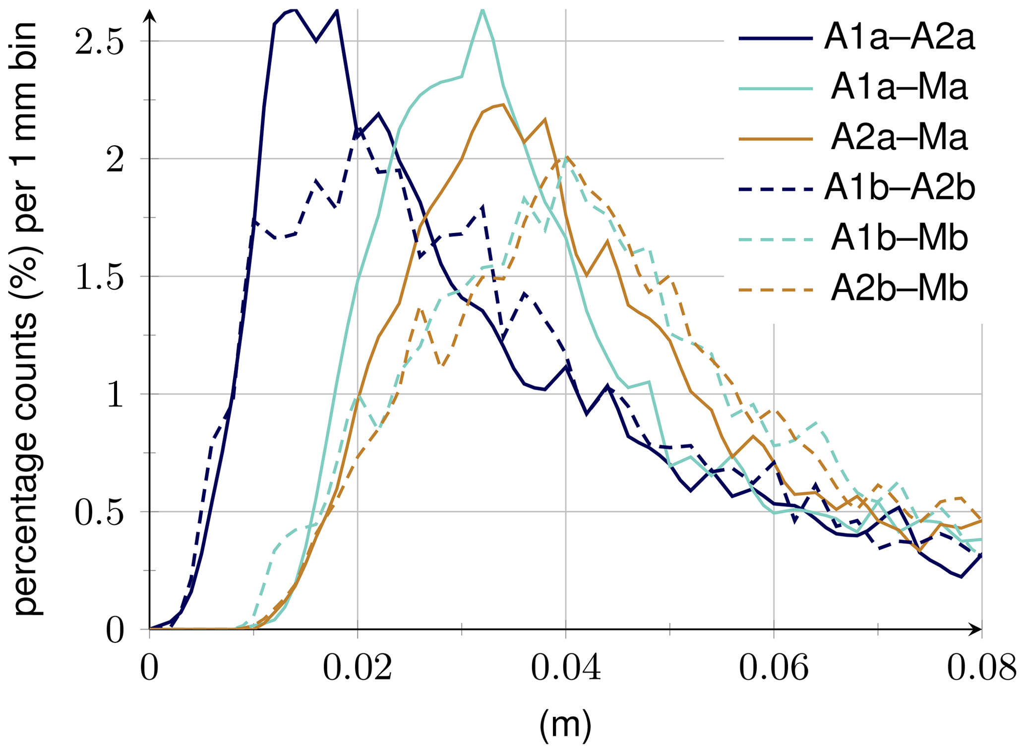
Figure 15 Histograms of the temporal rms of differences between various versions of firn thickness variations assessed at each grid cell of basin 3.

5.3 Firn model errors

Firn model errors arise from firn signals that are not simulated or not correctly represented by the firn model or its input from RCMs and reanalysis data. They are partly reflected in the differences of fv^Ma−fv^Mb (Fig. S16) and the adjustments over the firn models, i.e. any version of fv^A−fv^M (Fig. S17). Partly, the adjustments also include altimetry errors, as discussed in Sect. 5.4. Firn models generally show a smoother, more blurred spatial pattern than altimetry (cf. Fig. 6d–f versus a–b and also Fig. 7b versus a). Reasons may be small-scale, mainly wind-driven processes that are missing in the model physics or not resolved at the same level of detail due to the coarser spatial resolution of the models (Lenaerts et al., 2012, 2019).

The spatial patterns of absolute differences within fv^M and of the adjustments (e.g. Fig. 7c) follow the spatial pattern of the signal itself. The greatest differences occur at the margins, where the climate is wetter and temperatures and accumulation are higher than inland. Especially in these coastal regions of high-relief topography, the horizontal resolution of the models, probably together with its physics, plays an important role (Mottram et al., 2021). There, the differences between altimetry and firn models may be influenced by an incorrect or inaccurate spatial distribution of the modelled firn thickness variations (Fig. 6).

The modelled SMB components and their uncertainties have a direct impact on the modelled firn thickness. By assessing the spread of an ensemble of modelled firn thickness changes, Verjans et al. (2021) identified the RCMs as the largest contributor to the ensemble uncertainty. A precise parameterisation of firn compaction and surface snow density gains in importance in regions with high snowfall and large spatial variability in climatic conditions, such as Dronning Maud Land and Enderby Land (Verjans et al., 2021). However, the firn compaction rate in both firn models used here is determined by constant mean annual accumulation and not by instantaneous overburden pressure. This lessens the modelled firn compaction variability compared to the actual variability, potentially across all the areas of large accumulation variability (Kuipers Munneke et al., 2015).

In a relative sense, the adjustments (e.g. Fig. 7d) generally increase from the coast to the EAIS interior as the magnitude of the signal, the firn thickness variation, is very small in the interior due to the cold and dry climate. In these areas of low snowfall, the relative uncertainties in the firn models are virtually unaffected by the formulation of firn densification and surface snow density, but the input of RCM components is essential (Verjans et al., 2021). Scambos et al. (2012) argue that RCMs might overestimate SMB in wind-glazed areas. These areas feature wind-polished glazed surfaces at the top of a coarsely recrystallised firn layer and are formed by constant katabatic winds. They have near-zero SMB and occur on leeward faces of ice sheet undulations and megadunes (Scambos et al., 2012). Large wind-glazed areas are located across basins 4 and 8, where all four versions of adjustments reveal highest relative values (Fig. S17e–h).

In basin 4, towards the boundary with basins 1 and 3, the large relative adjustments (Fig. S17e–h) indicate disagreement between the models and altimetry, whereas the four versions of altimetry agree (Fig. S15i–l) and the two models agree (Fig. S16d). The reasons for this are not yet clear. Basin 8 is characterised by large megadune fields (Fahnestock et al., 2000; Dadic et al., 2013). Megadunes typically have an amplitude of 2 to 4 m and wavelengths of 2 to 5 km and are formed by a complex interaction of surface topography, snow accumulation, and redistribution due to highly persistent katabatic winds. While leeward slopes are wind glazed, windward slopes accumulate and are characterised by sastrugi of up to 1.5 m in height (Fahnestock et al., 2000; Frezzotti et al., 2002). The discrepancy between altimetry and the firn models across basin 8 can partly be explained by the lack of modelling of the formation of the complex spatial pattern of megadunes and their migration over time in the firn models. In the case of basin 8, models and altimetry disagree (Fig. S17e–h), as do the different versions of fv^M (Fig. S16d) and the different versions of fv^A (Fig. S15i–l). The latter is discussed in Sect. 5.4.

Discrepancies within the adjustments (i.e. within versions of fv^A−fv^M) can further indicate which firn model or which dominant patterns of one firn model fits the altimetry better. Overall, the adjustments are smaller when involving Ma (Fig. 8, Table 2). Amongst the different basins (see Figs. S28 and S29, solid green and brown versus dash-dotted green and brown lines), this applies in particular for basins 4–6. Across basin 2 the adjustments tend to be slightly smaller when involving Mb. Altimetric residuals, r^A, still include a non-negligible part (60 % for A1a) of the variance of altimetric variations (Fig. 9c, Table 3). Since the dominant patterns were chosen such that they cover at least 90 % of the variance of fv^M, r^A could partially contain real firn signals captured by firn models in the remaining ∼10 % of the data variance. However, it is likely that a larger part of r^A includes real firn signals not captured by the dominant temporal patterns of the firn models. The PSD of the underlying time series of r^A1a yields a spectral index of −1.7 (Sect. 4.3, Fig. 10b). The remaining autocorrelation in the residuals suggests that temporally correlated signals such as real firn signals are still present. Also, the spatial patterns of the most dominant modes of r^A reveal topography-dependent magnitudes and patterns, as one would expect from SMB and its variations (Sect. 4.4, Fig. 11a–c). Besides firn signals, the altimetric residuals additionally include altimetry errors (discussed in Sect. 5.4) and probably also further signals related to variations in ice flow dynamics or subglacial hydrology (not discussed further).

5.4 Altimetry errors

The differences between any version of fv^A and fv^M (the adjustments, e.g. Fig. 7c) may include effects of altimetry errors, in addition to firn model errors. Noise in the altimetry measurements might explain another part of the fact that firn models show a smoother spatial pattern of variations than altimetry. Noise in altimetry can be a problem, especially in the interior of the EAIS, where the signal-to-noise ratio is low. Over megadune areas (widely located in the interior across basin 8), conventional radar altimetry with pulse-limited footprints of 1.5 to 2.5 km in diameter may not be capable of adequately observing the time-varying spatial patterns of megadunes.

A further limitation in radar altimetry is that measurements refer to the local topographic maxima within their footprints. Especially at the margins over complex topography, this can lead to sampling issues, as the elevation changes acquired there cannot capture the larger changes often found in the valleys. Laser altimeters are not affected by this sampling issue. However, since ICESat operated in the campaign mode (Abshire et al., 2005), the sampling in areas with steep slopes can vary strongly during the period 2003–2009, with some months including laser altimetry and some months relying exclusively on radar altimetry. Moreover, radar altimetry results are affected by the time-varying radar waveform shape due to time-varying signal penetration (Davis and Ferguson, 2004; Rémy et al., 2012). Even though these effects are accounted for in the altimetry processing, related residual errors may have an impact on the adjustments. These errors, which tend to be correlated in time, are likely included in the altimetric residuals, r^A, which may explain, to some part, the temporal correlation of r^A (Sect. 4.3, Fig. 10b).

Discrepancies within the adjustments (i.e. within versions of fv^A−fv^M) can indicate which altimetry solution is closer to the firn models. However, results are equivocal (Fig. 8, Table 2). When involving the Ma firn model, the adjustments through A1 are smaller than those through A2 for most basins (see Figs. S28 and S29, solid green versus solid brown line). When involving the Mb firn model instead, the adjustments are of the same order of magnitude for A1 and A2, and it depends on the basin whether the adjustments are smaller with A1 or A2.

Uncertainties due to a different analysis of the altimetry measurements are reflected by the differences in fv^A (Fig. 14b) and r^A (Fig. 14d) between solutions based on the same firn model (A1a–A2a or A1b–A2b). The median values (over all grid cells) of rms differences of r^A1a−r^A2a in the time period after 2003 are ∼4.9 cm and ∼96 %, in an absolute and relative sense, respectively. If the entire period was considered, the median values would increase considerably (∼7.3 cm and ∼163 %). For both periods, the residual differences are greater than the differences of fv^A1a−fv^A2a (Table 2, Fig. 14b) and also greater than the uncertainty estimate of fv^A (Sect. 5.2, Fig. 14c).

The differences between fv^A1 and fv^A2 as well as between r^A1 and r^A2 mostly result from the combined effect of the various differences between the altimetry analysis of Schröder et al. (2019a) and Nilsson et al. (2022) (Sect. 2.1). The rms of fv^A1a−fv^A2a is shown in Fig. 14b in a relative sense. The largest relative differences occur in regions of complex topography, such as in Victoria Land (at the margin of basin 7); next to the Amery Ice Shelf (at the margin of basin 4); and over most of basin 8, for which we already discussed the possible influence of megadunes. In addition, stripes related to the satellite ground tracks are visible in the region of basins 1 to 2 (Fig. 14b). They seem to appear predominantly in fv^A2 (Fig. S15b and d).

The following features may likely be quite clearly attributed to a difference in intermission and intermode calibration between the two altimetry products. The mode change of CryoSat-2 (see e.g. Fig. 5 in Slater et al. (2018) for the mode boundaries) is reflected in the residual differences (Fig. 14d). Here, the main influence seems to come from A2 altimetry, as the areas at the mode boundary in basins 5–7 and 9–10, characterised by a higher rms value, are mainly visible in r^A2 (Fig. S18f and h). In addition, the mode transition also appears to be reflected in fv^A2, particularly at basins 5 and 6 (Fig. S15b and d). The PCA carried out on r^A1a−r^A2a and r^A1b−r^A2b reveals a prominent drop between July 2010 and January 2011, together with overall linear trends before and after this drop in the first PC (Fig. 12d). The corresponding spatial pattern (Fig. S26a and b) is most pronounced and coherent over the EAIS. The pattern of the first mode is an indicator for differences and uncertainties in deriving intermission offsets, as CryoSat-2 measurements begin in July 2010. The errors in the altimetry are not only seen in the first modes of the PCA of the residual differences. It is likely that the first modes of the PCA of the residuals themselves also contain altimetry errors. A comparison of the dominant modes of the residuals (Fig. 11) with those of the residual differences (Fig. 12) indicates partly similar features, which suggests similar causes. For example, there are also remarkably large fluctuations in the first temporal patterns of the residuals between July 2009 and January 2011 (Fig. 11d).

5.5 Limitations of the approach

In regions of a low signal-to-noise ratio the regression approach has a limited capability to distinguish between signal and error. This applies in particular to the interior of the EAIS (basin 8 and parts of basins 1 and 4). In these areas, the regression of the altimetry data to PC^M may be dominated by noise in the altimetry data. In this study, we work with a constant spatial grid resolution of 10 km × 10 km regardless of the signal magnitude. To improve the signal-to-noise ratio, further work may choose a geographically varying spatial resolution adapted to the spatial variability in the glaciological processes, which would probably imply a coarser resolution in the interior.

We included altimetry measurements only over the period May 1992 to December 2017 as this represents the common period of both altimetry products (Sect. 2). A2 altimetry data, however, are available until December 2020. Further investigations may hence extend the period to the more recent past. These may incorporate accurate laser measurements from ICESat-2 characterised by a low noise level and near-zero signal penetration (Nilsson et al., 2022; Otosaka et al., 2023a).

The stochastic model in the regression approach does not include temporal error covariances in altimetry (Sect. 3.3), although errors in the altimetry time series exhibit temporal correlations, as shown by Ferguson et al. (2004) and also in this study (Sect. 4.3). The consideration of temporal correlations is essential for assessing more realistic uncertainties. In particular, this is the case for long-term trends (Williams et al., 2014). Thus, future work may extend the stochastic model. This requires a comprehensive error characterisation for altimetry products, which has not been provided up to now. An empirical error characterisation could apply different noise models (e.g. power law, generalised Gauss–Markov, auto-regressive) to the regression approach (Bos et al., 2012; King and Watson, 2020). Alternatively, the spread of an ensemble of altimetry solutions could be considered (Willen et al., 2022).

5.6 Outlook

We do not aim here to compare our results with in situ data, as the ground-based SMB observations are mostly single-point measurements and have a very sparse spatial and temporal coverage (Eisen et al., 2008). However, future investigations may assess the benefits of fv^A in certain regions with in situ data, e.g. by making use of stake observations (Mottram et al., 2021; Richter et al., 2021).

To improve firn model outputs, it is important to refine the horizontal spatial resolution of RCMs and to simulate surface processes at a higher spatial resolution (Lenaerts et al., 2019). For Greenland, Noël et al. (2016) statistically downscaled outputs from RACMO2.3 at 5.5 and 11 km to a resolution of 1 km, which led to e.g. increased melt over certain areas. Similar work is in progress for Antarctica, downscaling RACMO2.3p2 at 27 to 2 km (Noël et al., 2023). Furthermore, a more detailed physical parameterisation of the processes already considered and the inclusion of processes not yet simulated can improve the models (Agosta et al., 2019; Gutiérrez et al., 2021). An update of RACMO2.3p2 to RACMO2.4p1 with enhanced physics is now available for 2006 to 2015. This includes several new and updated parameterisations, such as cloud, aerosol, and radiation schemes or a new scheme for spectral albedo and radiative transfer in the snow scheme (van Dalum et al., 2024).

To improve altimetry products, noise in the altimetry measurements and correlated altimetry errors related in particular to time-variable radar signal penetration and scattering effects need to be reduced. Helm et al. (2023) developed a new processing scheme (retracker) based on a deep convolutional neural network architecture, resulting in presumably strongly reduced time-variable signal penetration effects, which could significantly improve the elevation change products from the entire sequence of radar altimetry missions. Moreover, the intermission calibration needs further investigation. The patterns of estimated intermission offsets are spatially variant and are related to the waveform parameters, possibly associated with topography and surface properties. However, this relation is not fully understood, so no functional relationship has yet been found and intermission offsets are determined empirically (Zwally et al., 2005; Khvorostovsky, 2012; Schröder et al., 2019a; Nilsson et al., 2022). Therefore, intermission calibration still remains one of the most challenging processing steps for inferring a long-term, multi-mission satellite altimetry estimate.

Future developments in firn modelling, satellite altimetry analysis, and altimetry mission sensors will allow for identifying interannual firn signals and, thereby, better isolating and quantifying long-term trends. This will improve long-term estimates and reduce their uncertainties (Amory et al., 2024). The regression approach presented in this study may set the stage for isolating long-term signals in satellite altimetry from the large interannual variations. To this end, future studies should extend the approach with an appropriate stochastic model that accounts for covariances in altimetry to derive statistically significant long-term trends over 25 to 30 years. With longer time series, trend uncertainties will be further reduced (Wouters et al., 2013). In this way, large uncertainties in inferring mass balance estimates of the EAIS (Otosaka et al., 2023b) may be reduced and the question whether the EAIS is currently thickening or thinning (Nilsson et al., 2021) may be answered in the future.

6 Conclusions

We developed a new approach that combines satellite altimetry and firn modelling results to resolve Antarctic firn thickness variations at a high temporal and spatial resolution, namely by monthly 10 km grids. On the one hand, our approach incorporates the strengths of the firn models, above all the capability to capture the timing of firn thickness variations. On the other hand, our approach compensates for shortcomings of the firn models, foremost in the simulation of the location-dependent amplitudes of the variations. To do so, we fitted dominant temporal patterns of interannual to decadal variations in Antarctic firn thickness inferred from the firn models from Veldhuijsen et al. (2023) and Medley et al. (2022a) to satellite altimetry observations from Schröder et al. (2019a) and Nilsson et al. (2022). In this way, we generated a new, combined product, which we named the adjusted firn thickness variations, fv^A.

Our guiding question was as follows: how well can satellite altimetry and firn models resolve Antarctic firn thickness variations? Well, it depends. This study shows that firn models and altimetry products provide complementary information on firn thickness variations. The combined data set, fv^A, characterises spatially resolved variations better than either (1) firn models alone or (2) altimetry alone. (1) The adjusted firn thickness variations, fv^A, outperform the modelled firn thickness variations, fv^M. Compared with fv^M, fv^A improves the amplitudes of the variations because they are observed by the altimeter satellites and their patterns actually indicate more meaningful information. However, the improved observed amplitudes may also include effects of altimetry errors due to firn penetration, as both the time-variable signal and these errors are influenced by the SMB and firn processes and are thus temporally correlated. (2) The adjusted firn thickness variations, fv^A, outperform the altimetric variations, hv^A, because fv^A eliminates a large part of the altimetry errors. If one were to take hv^A alone, this would also incorporate all the errors in hv^A. Over Antarctica, or rather the entire area studied, this would introduce median absolute and relative uncertainties of ∼7.3 cm and ∼163 %, respectively (evaluated at the grid cell level). However, by choosing fv^A instead of hv^A, part of the observed firn signal is ignored.

How well fv^A resolves real Antarctic firn thickness variations depends strongly on the region under investigation. Over all grid cells of Antarctica, median absolute and relative uncertainties in fv^A are ∼4.2 cm and ∼80 %, respectively. Over all grid cells of individual basins, the median relative uncertainties are lowest for basin 5, the region of Queen Mary Land (54 %), and highest for basin 8 (186 %). The large uncertainty in basin 8 is likely due to the presence of megadune fields. We find the smallest adjustment that fv^A requires over fv^M when using the altimetry data from Schröder et al. (2019a) and the firn model of Veldhuijsen et al. (2023), and this is most prominent for basins 5 and 6. From the spectral analysis of the altimetry residuals, r^A, we still find autocorrelated signals that we could not attribute to firn thickness variations using the firn models. A small part of these residual signals may be due to the limitation of our regression which neglects up to 10 % of the potentially correctly modelled variations. However, we attribute the larger part to a combination of altimetry errors, in particular time-variable signal penetration and errors in intermission offsets, and firn model errors, that is, incorrectly simulated processes or missing processes.

We identified regions of discrepancy between the firn models and the altimetry products and within the models or altimetry and discussed the underlying errors in both the models and the altimetry. These results shall help modellers and altimetry data processors to improve their simulations and processing methods (Sect. 5.6) and help users to better understand the nature of the modelling and altimetry data and to apply and interpret them, knowing their strengths and limitations.

Appendix A: Impact of methodological changes

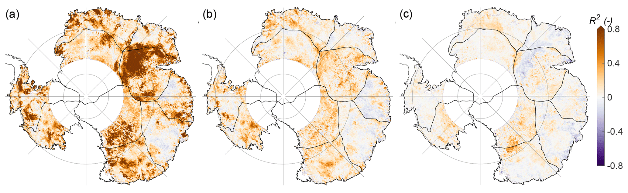
Figure A1 Differences between the R-squared values from A1a and the experiments E1, E2, and E3. (a) A1a−E1, (b) A1a−E2, (c) A1a−E3. Colour bar arrows indicate that the value range exceeds the limits of the colour scale.

A1 Methods

To investigate the impact of methodological changes on determining adjusted firn thickness variations, fv^A, three modifications to the original regression approach are tested.

In the first experiment, E1, we simply subtract the modelled firn thickness variations, fv^M, from the altimetric variations, hv^A, according to

$$\begin{array}{}\text{(A1)}& {\displaystyle }{r}^{\mathrm{E}\mathrm{1}}\left(t\right)={\mathrm{hv}}^{\mathrm{A}}\left(t\right)-{\mathrm{fv}}^{\mathrm{M}}\left(t\right).\end{array}$$

In the second experiment, E2, fv^M at any grid cell is simply scaled to fit the altimetric variations. The regression reads

$$\begin{array}{}\text{(A2)}& {\displaystyle }{\mathrm{hv}}^{\mathrm{A}}\left(t\right)=e{\mathrm{fv}}^{\mathrm{M}}\left(t\right)+r^{\mathrm{E}\mathrm{2}}\left(t\right),\end{array}$$

where e is the scaling factor. We refer to e fv^M=fv^E2 as scaled firn thickness variations. In the third experiment, E3, we do not change the principle of the deterministic model of Eq. (1), but we modify the dominant temporal patterns, PC^M. Originally, the temporal patterns are derived from the standardised fv^M by PCA. In E3, the time series of fv^M are not standardised prior to the PCA. The resulting modified adjusted firn thickness variations are referred to as fv^E3.

We consider the regression method whose R-squared value, R², is maximum best, i.e. which is able to describe most of the data variance. For the three experiments, Eq. (3) modifies to

$$\begin{array}{}\text{(A3a)}& {\displaystyle }{R}_{\mathrm{E}\mathrm{1}}^{\mathrm{2}}& {\displaystyle }=\mathrm{1}-{\displaystyle \frac{\mathrm{SS}\left(r^{\mathrm{E}\mathrm{1}}\right)}{\mathrm{SS}({\mathrm{fv}}^{\mathrm{Ma}}+r^{\mathrm{E}\mathrm{1}})}},\text{(A3b)}& {\displaystyle }{R}_{\mathrm{E}\mathrm{2}}^{\mathrm{2}}& {\displaystyle }=\mathrm{1}-{\displaystyle \frac{\mathrm{SS}\left(r^{\mathrm{E}\mathrm{2}}\right)}{\mathrm{SS}(e{\mathrm{fv}}^{\mathrm{Ma}}+r^{\mathrm{E}\mathrm{2}})}}=\mathrm{1}-{\displaystyle \frac{\mathrm{SS}\left(r^{\mathrm{E}\mathrm{2}}\right)}{\mathrm{SS}({\mathrm{fv}}^{\mathrm{E}\mathrm{2}}+r^{\mathrm{E}\mathrm{2}})}},\text{(A3c)}& {\displaystyle }{R}_{\mathrm{E}\mathrm{3}}^{\mathrm{2}}& {\displaystyle }=\mathrm{1}-{\displaystyle \frac{\mathrm{SS}\left(r^{\mathrm{E}\mathrm{3}}\right)}{\mathrm{SS}({\mathrm{fv}}^{\mathrm{E}\mathrm{3}}+r^{\mathrm{E}\mathrm{3}})}}.\end{array}$$

A2 Results

The impact of methodological choices on the goodness of fit is tested based on the three experiments, E1–E3 (Sect. A1). The results are given for using the Ma firn model and A1 altimetry and should, therefore, be compared to the results from the regression approach A1a.

Table A1 Explained variance or R² for each basin and each experiment (E1, E2, E3) of methodological changes to the regression approach over the period after 2003. R² is first calculated for each grid cell according to Eqs. (A3a)–(A3c) and after averaged over each basin. Values of $\stackrel{\mathrm{‾}}{\mathrm{E}\mathrm{1}}$, $\stackrel{\mathrm{‾}}{\mathrm{E}\mathrm{2}}$, and $\stackrel{\mathrm{‾}}{\mathrm{E}\mathrm{3}}$ are calculated by first averaging the results from the experiments over each basin and then applying Eqs. (A3a)–(A3c).

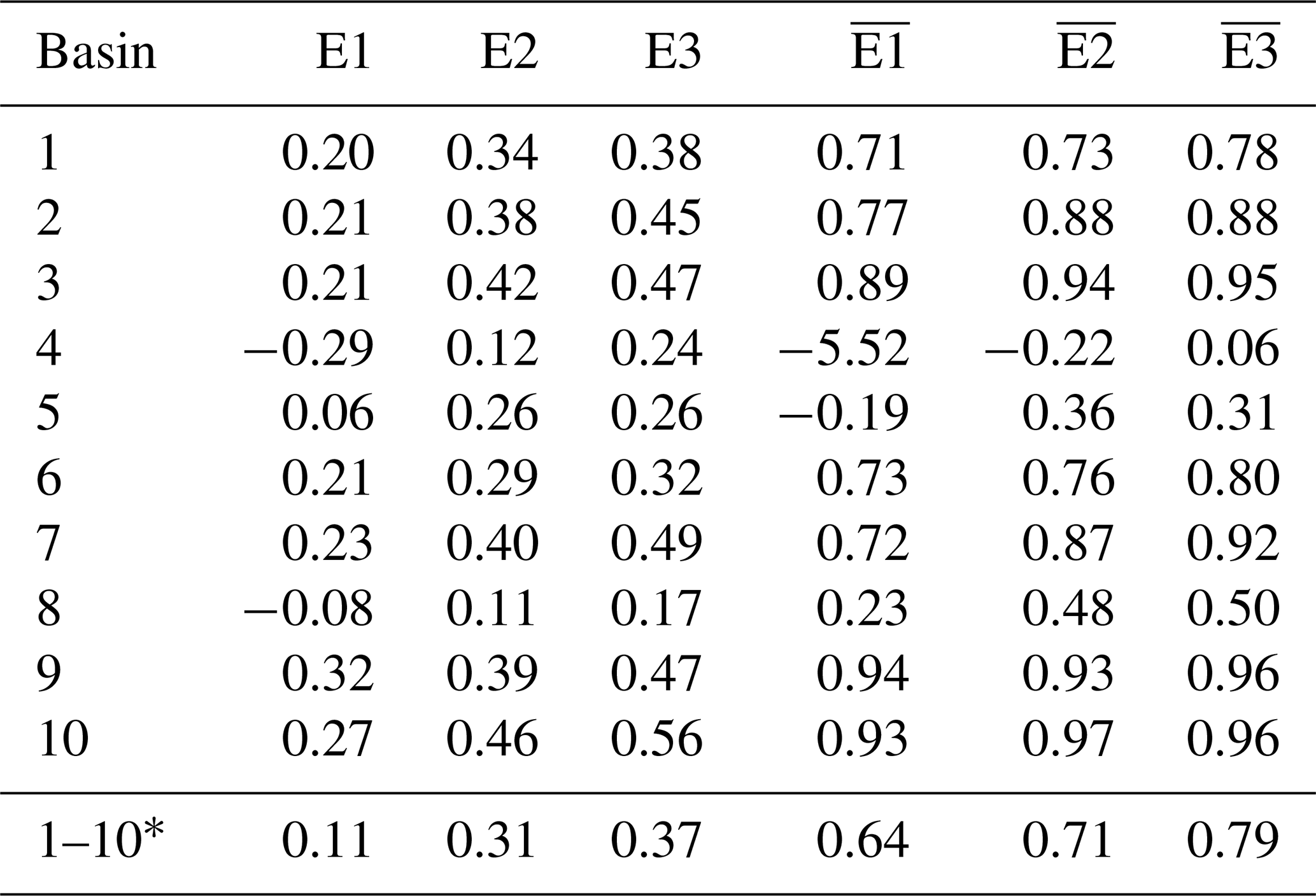
^* Refers to the entire area (considered a single basin).

For every grid cell, Fig. A1 compares the R-squared values from the regression approach A1a, $R_{\mathrm{A}\mathrm{1}\mathrm{a}}^{\mathrm{2}}$, to the R-squared values $R_{\mathrm{E}\mathrm{1}}^{\mathrm{2}}$, $R_{\mathrm{E}\mathrm{2}}^{\mathrm{2}}$, and $R_{\mathrm{E}\mathrm{3}}^{\mathrm{2}}$. $R_{\mathrm{A}\mathrm{1}\mathrm{a}}^{\mathrm{2}}$ is larger than $R_{\mathrm{E}\mathrm{1}}^{\mathrm{2}}$, $R_{\mathrm{E}\mathrm{2}}^{\mathrm{2}}$, and $R_{\mathrm{E}\mathrm{3}}^{\mathrm{2}}$ over 88 %, 78 %, and 66 % of the total area, respectively. After calculating $R_{\mathrm{E}\mathrm{1}}^{\mathrm{2}}$, $R_{\mathrm{E}\mathrm{2}}^{\mathrm{2}}$, and $R_{\mathrm{E}\mathrm{3}}^{\mathrm{2}}$ for each grid cell, (basin-)mean values are derived and listed in columns 2–4 of Table A1. Averaged over the entire area, E1, E2, and E3 have mean R² values of 0.11, 0.31, and 0.37. For all three modifications, R² is smaller than $R_{\mathrm{A}\mathrm{1}\mathrm{a}}^{\mathrm{2}}$ (Table 3, column A1a), and, thus, their regression approaches describe less of the data variance than the original regression approach of A1a. E3 describes slightly more of the data variance than A1a for 1 out of 10 basins (basin 3: 47 % versus 45 %). Moreover, Table A1 (columns 6–7) lists values of R² derived from basin-average time series ($\stackrel{\mathrm{‾}}{\mathrm{E}\mathrm{1}}$, $\stackrel{\mathrm{‾}}{\mathrm{E}\mathrm{2}}$, and $\stackrel{\mathrm{‾}}{\mathrm{E}\mathrm{3}}$). Values derived from basin-average time series are larger than values based on the calculations per grid cell, similar to the regression approach A1a (Table 3, column $\stackrel{\mathrm{‾}}{\mathrm{A}\mathrm{1}\mathrm{a}}$ versus A1a).

The simple scaling factor, e, adjusted during the regression approach after experiment E2 is displayed in Fig. S30.