How many parameters are needed to represent polar sea ice surface patterns and heterogeneity?

Sea ice surface patterns encode more information than can be represented solely by the ice fraction. The aim of this paper is thus to establish the importance of using a broader set of surface characterization metrics and to identify a minimal set of such metrics that may be useful for representing sea ice in Earth system models. Large-eddy simulations of the atmospheric boundary layer over various idealized sea ice patterns, with equivalent ice fractions and average floe areas, demonstrate that the spatial organization of ice and water can play a crucial role in determining boundary layer structures. Thus, various methods used to quantify heterogeneity in categorical lattice-based spatial data, such as those used in landscape ecology and Geographic Information System (GIS) studies, are employed here on a set of recently declassified high-resolution sea ice surface images. It is found that, in conjunction with ice fraction, patch density (representing the fragmentation of the surface), the splitting index (representing variability in patch size), and the perimeter–area fractal dimension (representing the tortuosity of the interface) are all required to describe the two-dimensional pattern exhibited by a sea ice surface. For surfaces with anisotropic patterns, the orientation of the surface relative to the mean wind is also needed. Finally, scaling laws are derived for these relevant landscape metrics, allowing for their estimation using aggregated spatial sea ice surface data at any resolution. The methods used in and the results gained from this study represent a first step toward developing further methods for quantifying variability in polar sea ice surfaces and for parameterizing mixed ice–water surfaces in coarse geophysical models.

1 Introduction

The polar sea ice surface, a sensitive indicator of global climate change, exhibits persistent biases in sea ice fraction and extent in coarse-resolution Earth system models (ESMs) (Liu et al., 2022; Casagrande et al., 2023; Myksvoll et al., 2023). Among other factors, these biases result from the inability of ESMs to resolve fine-scale spatial variability in sea ice and the resulting exchanges with the ocean below (Ramudu et al., 2018) and the atmosphere aloft (Bates et al., 2006; Esau, 2007). The effect of this subgrid-scale sea ice variability is typically parameterized in climate models using the ice fraction (f_i) as the sole surface composition characteristic. Usually, either an equivalent homogeneous surface or mosaic flux aggregation is used (Elvidge et al., 2016; Bou-Zeid et al., 2020; Elvidge et al., 2021), but both yield an average flux, weighted by the ice and water fractions, that is inaccurate as the flux does not account for the impact of surface heterogeneity on the dynamics of the lower atmosphere and the nonlinear interactions with airflow above the ice and water (de Vrese et al., 2016; Lüpkes et al., 2012). This incomplete representation of sea ice surfaces and boundary layer structures results in errors in the turbulent exchanges of heat, moisture, and momentum across polar sea ice surfaces (Nilsson et al., 2001; Bourassa et al., 2013; Taylor et al., 2018). The dynamics and secondary circulations below the first vertical grid cell level in climate models are particularly underresolved, and they have a direct impact on air–surface exchanges; it is thus imperative to understand how these features influence fluxes (Mahrt, 2000; Essery et al., 2003; de Vrese et al., 2016). These gaps in representing fine-scale dynamics and fluxes propagate to the projection of future changes in the Arctic climate system and the resulting surface energy budget (Persson et al., 2002; Miller et al., 2017), which may be one reason why climate model ensembles consistently underpredict Arctic sea ice sensitivity to surface temperature warming. This underprediction has persisted throughout the last three Intergovernmental Panel on Climate Change (IPCC) model development cycles (Stroeve et al., 2007; Rosenblum and Eisenman, 2016, 2017; Notz and Community, 2020). The resulting uncertainty in the ability of climate models to predict future sea ice evolution hinders effective action and decision-making; therefore, improving these models is imperative (Notz and Stroeve, 2018; Docquier and Koenigk, 2021).

The fringe zone that separates densely consolidated sea ice from the open ocean is known as the marginal ice zone (MIZ) – see Dumont (2022) for a review of the current state of MIZ research. In the MIZ, the size and organization of sea ice floes and water are influenced by winds, sea currents, waves, and material ice properties (Wang et al., 2016; Ren et al., 2021; Herman et al., 2021; Hwang and Wang, 2022). What makes this region unique is that near-surface air temperatures may fall between the surface temperatures of sea ice and water, resulting in abrupt spatial transitions between stabilizing and destabilizing surface buoyancy fluxes (Lüpkes et al., 2012). Such transitions produce drastically different turbulence-mean-based nonequilibrium dynamics and timescales (as demonstrated for comparable land–water transitions by Allouche et al., 2021, 2023b), all of which affect the surface–atmosphere exchanges between air, water, and sea ice. The ice fraction (f_i) in the MIZ ranges from 15 % to 80 % (Strong et al., 2017); however, any region of fractured sea ice gives rise to these abrupt transitions. It is precisely in these regions where the linear-weighted, averaged approaches described above will be most inadequate and where surface transitions will play a key role in the dynamics. Thus, it is important to devise better methods for quantifying the heterogeneity of a surface, characterizing its patterns, and encoding this information into coarse-resolution ESMs to better represent the polar environment.

To this end, the complex geometric patterns formed by sea ice floes need to be analyzed. Larger floes will have a proportionally greater effect on surface–atmosphere fluxes, whereas smaller floes, with their more frequent transitions, will exacerbate the nonlinearity of the exchange processes. These surface–atmosphere fluxes have a large effect on the atmospheric boundary layer (ABL) overlaying the marginal ice zone (MIZ-ABL). As a thought experiment, we can consider an ice–water surface with a very fine checkerboard pattern and a sea ice fraction (f_i) of 0.5; this configuration will lead to statistically homogeneous ice floes that are locally variable at the surface but effectively homogeneous with respect to the MIZ-ABL, where turbulence rapidly mixes the floes' small-scale signatures (Brutsaert, 2005; Mahrt, 2000; Bou-Zeid et al., 2004). However, two large patches of sea ice and water (meso-α heterogeneity; see Bou-Zeid et al., 2020), which also have a sea ice fraction (f_i) of 0.5, will generate significant circulation closer to that of a sea breeze due to the abrupt transition between the two large, homogeneous surfaces (Porson et al., 2007; Crosman and Horel, 2010; Allouche et al., 2023a). The dynamics and thermodynamics in this MIZ-ABL system, and the surface exchange therein, will thus be quite different for these two patterns, even if some key surface properties, e.g., temperature and roughness, are identical (Bou-Zeid et al., 2007).

Given the importance of the topic and the challenges outlined above, previous work has attempted to quantify the heterogeneity of sea ice surfaces (Wenta and Herman, 2018, 2019; Michaelis et al., 2020; Horvat, 2021; Dumont, 2022), utilizing surface and meteorological properties like sea ice fraction, geostrophic velocity, lead width, and floe size distribution. Furthermore, parameterizations for flow over leads in sea ice have been developed based on non-eddy-resolving models (Lüpkes et al., 2008; Michaelis et al., 2021). Michaelis and Lüpkes (2022) also a conducted turbulence parameterizations (based on large-eddy simulation models) over ensembles of leads, but they used a two-dimensional ice fraction geometry and a higher ice fraction. However, the small-scale patterns in the MIZ require broader and more versatile methods of heterogeneity characterization (e.g., Mandelbrot, 1967), especially as the resolution increases. In addition, the computational grid of even the highest-resolution weather or climate model cannot resolve all the spatial features in the MIZ. One thus needs to consider how to represent unresolved surface characteristics in such models; these characteristics can be thought of as lattice-type spatial structures, as defined by Cressie (1993). Observational data of MIZ ice patterns also have a finite resolution and are thus comparable to lattice data, allowing for the use of different metrics specifically defined for lattice surfaces and offering ways to characterize the heterogeneity patterns of these polar surfaces. In this paper, we examine approaches for this quantification that are commonly used in landscape ecology, a field that has generated a multitude of methods to study lattice spatial data (Li and Reynolds, 1994, 1995; Pickett and Cadenasso, 1995).

Studies in landscape ecology have previously sought an optimal independent group of metrics for understanding the heterogeneity of lattice surfaces. Riitters et al. (1995) used multivariate factor analysis to suggest six groups of metrics, including image texture, average patch compaction, and average patch shape. Cushman et al. (2008) used principal component analysis to propose seven broad metrics at the landscape level, including contagion, large-patch dominance, and proximity (see Table 9 in the aforementioned study). For the two-dimensional, binary sea-ice–water surfaces considered in this study, we chose the variance inflation factor (VIF) technique to reduce these metrics to a compact set of metrics that are weakly dependent on one another, minimizing information redundancy (Miles, 2014).

The questions that will be answered in this study are as follows:

1. Is the sea ice fraction of a MIZ surface, combined with some measure of average floe area, sufficient to predict the behavior of the overlying MIZ-ABL?

2. If not, what other surface information in a two-dimensional, lattice-based spatial pattern is needed to describe air–sea interactions?

3. How can this surface information be applied to sea ice surfaces in weather models and ESMs, considering factors such as availability of information, resolution-resampling invariance, and ease of understanding?

Section 2 details the methods employed for the idealized and real-world maps used in this study, including the steps taken to reduce multicollinearity and determine which landscape metrics, alongside sea ice fraction, provide additional information on the pattern of the sea ice surface. The large-eddy simulations used are also presented in this section, and a more complete description is found in Appendix A and B. Section 3 reports the results of the idealized sea ice surfaces in the large-eddy simulation, thereby answering the first of our questions and setting the stage for the remaining questions. Section 4 presents the results from the 2D surface analysis, thereby answering the second and third questions, with additional discussion on principal directions and climate model implications found in Sect. 5. Section 6 synthesizes the findings and outlines open questions to guide future investigations of sea ice heterogeneity.

2 Methods and data

2.1 Large-eddy simulations

Large-eddy simulations (LESs) of the MIZ-ABL were conducted for different idealized configurations of sea ice. LESs are widely used to model heterogeneous high-Reynolds-number flows (Baidya Roy, 2002; Bou-Zeid et al., 2004) in, for example, convective boundary layers (Courault et al., 2007; Maronga and Raasch, 2013), stable boundary layers (Huang et al., 2011), and coastlines (Allouche et al., 2023a) – see Sect. 3.6 of Stoll et al. (2020). This heterogeneous high-Reynolds-number description aptly applies to the MIZ-ABL. Unlike direct numerical simulations (DNSs), LESs are able to attain a Reynolds number (Re) representative of the MIZ-ABL (∼10⁷) because the smaller turbulent eddies (smaller than the filter size, which is comparable to the numerical grid spacing in our simulations) are not explicitly resolved. However, unlike Reynolds-averaged Navier–Stokes (RANS) approaches, which encompass all weather and climate models, LESs directly resolve and capture large turbulent eddies, the heterogeneity of the surface, advective fluxes, and large-scale sea ice patterns, making them a computationally and physically appealing approach for the problem at hand. By retaining these larger structures, most of the turbulent energy and fluxes are explicitly resolved, allowing for the investigation of three-dimensional flow structures that may arise over these heterogeneous surfaces.

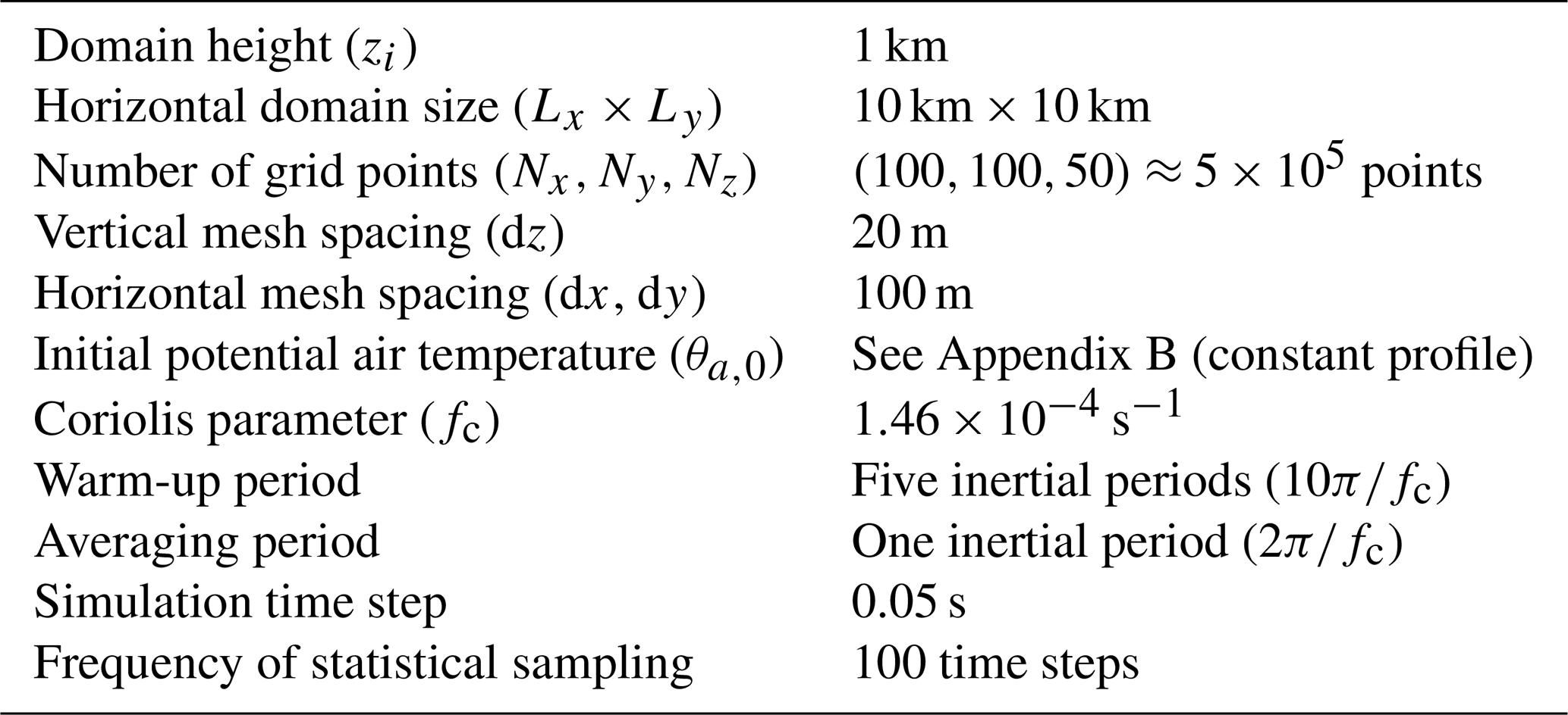
Table 1 Numerical details of the large-eddy simulation. Time is represented in terms of inertial periods ($\mathrm{2}\mathit{\pi }/f_{\mathrm{c}}$), indicating the timescale associated with the response of the mean flow. This timescale represents the Coriolis redistribution of energy between u and v (Momen and Bou-Zeid, 2016).

LESs are thus used to model MIZ-ABL flow over 10 km × 10 km patterns of idealized ice–water surfaces, modulated by a Coriolis force at a latitude (Φ) of 90° N in a horizontally periodic domain, yielding a Rossby number (Ro) of 13.7 (see Fig. 1). We note that simulations using the same Ro value, even those conducted at lower latitudes with mean wind speeds, would give similar results – see the dimensional analysis of flow over heterogeneous surfaces in Fogarty and Bou-Zeid (2023a) and Allouche et al. (2023a). This full domain is smaller than a single grid cell in state-of-the-art ESMs, underlining why simulated properties of the MIZ-ABL in ESMs require subgrid-scale (SGS) parameterizations. For leads with a width of ∼1 km, a grid spacing of 10–20 m is usually chosen after grid convergence tests (Lüpkes et al., 2008; Gryschka et al., 2023). Our choice of a coarser horizontal resolution of 100 m reflects our aim of zooming out from a typical lead and examining the MIZ as a whole (which is also reflected in the horizontally periodic nature of the domain). A finer resolution in our simulations, while possibly improving the representation of turbulence and plume dynamics, may sacrifice some of the large scales and secondary circulations that arise from these heterogeneous surfaces, which we aim to capture with a large domain. The coarse resolution also does not compromise our ability to answer the first question because, as shown later, the differences in the dynamics between simulations with identical ice fractions but different surface patterns are significant and far exceed any plausible impact resulting from grid resolution. The simulations in this section are meant to demonstrate the need for surface analysis, given a constant ice fraction and an average ice floe area; thus, we do not focus on the quantitative aspects of the output. See Table 1 for all details of the simulations in this study; more information on the numerical aspects of our LES is provided in Appendix A.

The bottom-boundary condition for each simulation can be thought of in terms of categorical lattice-based spatial data, where each node represents either the ice class or the water class. An ice node is prescribed a surface temperature (θ_i) of 255 K, typical of fall and spring temperatures in the central Arctic, and a momentum roughness length of 1 mm, while a water node is prescribed a surface temperature (θ_w) of 271 K, roughly the freezing point of seawater, and a roughness length of 1 cm. The heat roughness length is set to 0.1 mm for the entire surface (both ice and water). There is a very large variability in roughness lengths in Arctic sea ice simulations (see Lüpkes et al., 2008; Andreas et al., 2010; Lüpkes et al., 2012; Elvidge et al., 2016; Gryschka et al., 2023), which reflects the physical differences between calm and stormy seas, as well as between new, flat ice and old ice that is deformed and refrozen. However, our choice of roughness lengths prioritized keeping constant ratios (which are the key dimensionless parameters influencing the results; Fogarty and Bou-Zeid, 2023a; Allouche et al., 2023a) among simulations to focus on the effect of sea ice patterns. Results with different values but the same ratios will lead to almost identical conclusions. In addition, sensitivity analyses (not shown here) indicated that the roughness lengths, even when their ratios were changed, had a very minor impact on the quantitative results compared to the temperature contrast, ice fraction, and ice–water patterns. The initial potential air temperature (θ_a,0), a constant profile, is defined so that the area-averaged sensible heat flux, as computed by the Monin–Obukhov surface flux parameterizations, is zero and thus lies between the ice and water surface temperatures (see Appendix B for details). The LES-modeled heat flux will, however, not be zero.

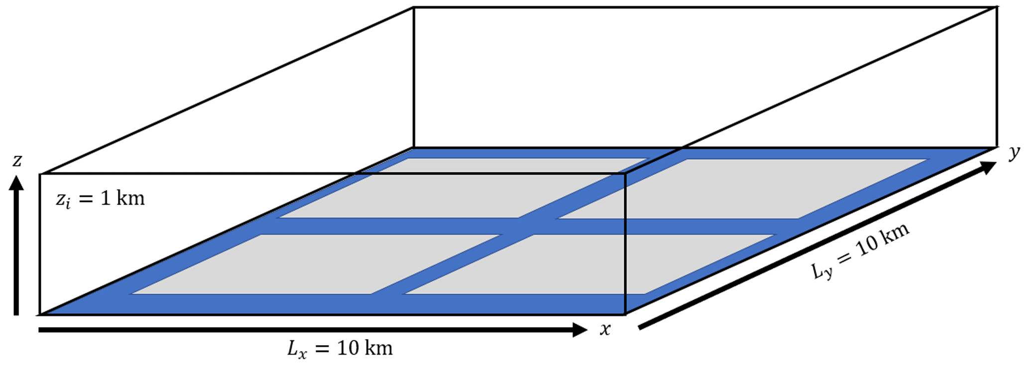
Figure 1 Schematic of the domain setup for the large-eddy simulation. The ice (in gray) has a surface temperature (θ_0,i) of 255 K and a roughness length (z_0,i) of 1 mm. The water surface (in blue) exhibits a θ_0,w value of 271 K and a z_0,w value of 1 cm. The bottom boundary represents one of the many cases (Pattern1) illustrated in Fig. 2.

All five patterns (Pattern1 to Pattern5), displayed in Fig. 2, were simulated. They have a fixed sea ice fraction (f_i) of 0.46 and a mean floe area of 11.56×10⁶ m². The geostrophic wind (M_g=2 m s⁻¹) flows from left to right at an angle of 18° relative to the x axis in all simulations. This is expected to give a surface wind (M₀) value that is roughly aligned with the x axis for homogeneous neutral surfaces due to Ekman veer (Ghannam and Bou-Zeid, 2021). These simulations are dry runs with no clouds present. The turbulence field is warmed up for about 60 h, and the statistics are then Reynolds-averaged over an additional 12 h. A variable with an overbar denotes averaging over time, which is used as a surrogate for ensemble Reynolds averaging, and any spatial averaging over the heterogeneous domain in x and y is indicated by angle brackets.

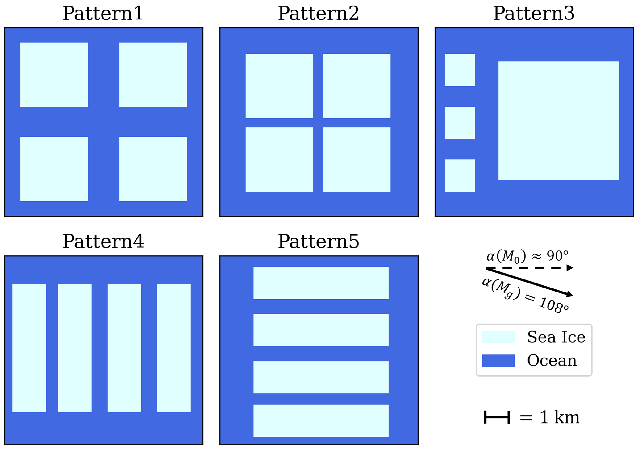
Figure 2 Bird's-eye view of the five idealized 10 km × 10 km sea ice surfaces created for the large-eddy simulation. The geostrophic wind (M_g) flows at an angle of 108°, resulting in the near-surface wind (M₀) flowing from left to right in all patterns. The results from the LES for these five patterns are discussed in Sect. 3.

In addition to the Rossby number and the roughness ratio discussed earlier, an important dimensionless input parameter in these simulations is the heterogeneity Richardson number, defined as

$$\begin{array}{}\text{(1)}& {\mathit{Ri}}_h={\displaystyle \frac{g}{{\mathit{\theta }}_{a,\mathrm{0}}}}{\displaystyle \frac{{\mathit{\theta }}_{\mathrm{w}}-{\mathit{\theta }}_{\mathrm{i}}}{M_{\mathrm{g}}^{\mathrm{2}}/z_{\mathrm{i}}}}.\end{array}$$

Ri_h encodes the competition between buoyancy-driven circulations generated by the surface temperature contrast and the uniform flow resulting from the synoptic forcing (M_g). All simulations in this study have equivalent inputs of Ri_h, Ro, and $z_{\mathrm{0},\mathrm{w}}/z_{\mathrm{0},\mathrm{i}}$. Based on previous dimensional analyses and LESs of flow over heterogeneous surfaces (Omidvar et al., 2020; Allouche et al., 2023a; Fogarty and Bou-Zeid, 2023a), matching these dimensionless inputs is required to be able to focus on the effects of surface sea ice fraction and patterns.

2.2 Ice map data

While the LES utilizes idealized surfaces to examine the influence of patterns on the MIZ-ABL, examining what other landscape metrics might be important for surface characterization necessitates the use of real-world sea ice maps. The lattice spatial data used in the statistical analysis (see Sect. 2.3) are derived from recently declassified high-resolution (1 m) Literal Image Derived Products (LIDPs) in accordance with national technical means (NTMs), as detailed in Kwok (2014). These images underwent a supervised maximum-likelihood classification algorithm, which assigned each pixel in the original LIDP to either a water class or an ice surface class (Fetterer and Untersteiner, 1998; Fetterer et al., 2008). This process converted the high-resolution LIDPs into categorical lattice-based spatial data, where each cell represents one of two possible surface types (ice or water).

These maps, which have a horizontal extent of up to 10 km by 10 km, comprise the dataset used to calculate the landscape metrics. Some of the images did not fully cover this full extent; thus, in order to retain the real-world sea ice geometry, we reflected the images onto areas with no data. All metric calculations and analyses were conducted on these modified surfaces. The advantage of this high-resolution, large-extent dataset is that we can analyze how these metrics change with grain size. These maps are thus aggregated from a 1 m resolution to 2 m, 10 m, 50 m, 100 m, 200 m, 500 m, 1 km, and 2 km resolutions; resampling was done using the nearest-neighbor method from the Python Imaging Library (PIL). These resolutions cover a range of common resolutions used in fine large-eddy simulations and numerical weather prediction (NWP) models. Due to the excessive computational-processing time required for the original 1 m resolution data, the highest resolution at which landscape metrics were calculated was 2 m.

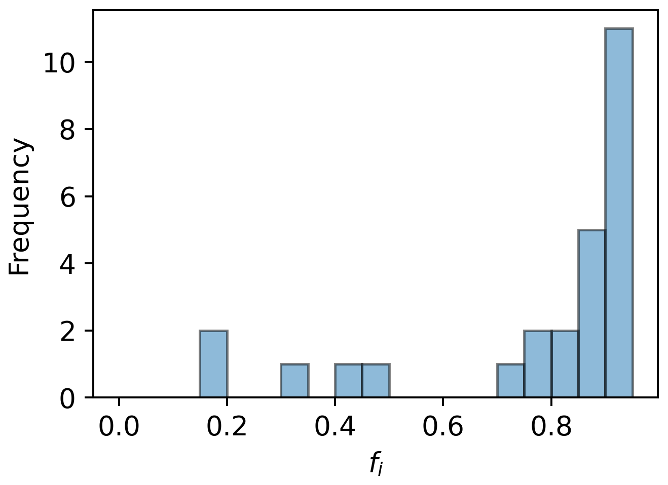
One important caveat of this dataset is that the histogram illustrating sea ice fraction (f_i) is heavily skewed toward higher sea ice fractions (see Fig. 3). We recognize that this may lead to bias in the results; however, the analysis methods developed here are insensitive to f_i and can certainly be applied to other datasets with more uniform sea ice fraction distributions in the future. The high resolution provided by the present dataset remains a key factor in its adoption for the present study since it allows us to aggregate and track how landscape metrics change from actual surface states when resampled to a coarser numerical grid.

Figure 3 The distribution of f_i values in the Fetterer et al. (2008) ice map dataset.

2.3 Landscape metric space reduction

FRAGSTATS, a spatial-pattern analysis program, was used to calculate landscape metrics (McGarigal and Marks, 1995) based on the lattice spatial data. When given GeoTIFF-format raster lattice data, FRAGSTATS calculates patch metrics, class metrics, and landscape metrics of your choice. Patch metrics are computed for each individual patch in the landscape and are thus not relevant for the current study of sea ice surface patterns. Class metrics are computed for each patch type (class) in the landscape. In this study, this would involve calculating metrics for sea ice only and water only. Although this metric may be useful in other applications of pattern analysis, in this study, we want to look at the aggregated patterns of sea ice and water combined. Thus, only landscape metrics were calculated. Sea ice fraction (calculated as the number of ice cells divided by the total number of ice and water cells) was calculated using the PIL as it is the only metric not provided by FRAGSTATS.

This resulted in 22 landscape metrics that focus on the global patterns of the surface. Many of these landscape metrics, however, are correlated with one another; for example, patch density and mean patch size are proportional to each other. This is due to the fact that there are limited observations one can make about a surface (such as the number of patches, the area of a patch, and the proportion of edge in a patch) but an infinite number of operations that can be performed on a surface. Therefore, many of these metrics (especially at the landscape level) simply represent different methods of aggregating or statistically analyzing these observations.

While collinearity between two metrics can be easily detected through a correlation matrix, multicollinearity (where one indicator is a linear combination of two or more other indicators) is more likely in these types of datasets. It is thus possible for two or more landscape metrics to jointly define another metric. An objective and statistical way of reducing these parameters is thus needed. Here, we chose the variance inflation factor (VIF),

$$\begin{array}{}\text{(2)}& {\text{VIF}}_{\mathrm{i}}={\displaystyle \frac{\mathrm{1}}{\mathrm{1}-R_i^{\mathrm{2}}}},\end{array}$$

where R² is the coefficient of determination, which is used to detect multicollinearity among these heterogeneity parameters (see Ibidoja et al., 2023). For each metric (X_i), when $i\in [\mathrm{1},\mathrm{\dots },\mathrm{22}]$, the VIF was calculated using a regression equation,

$$\begin{array}{}\text{(3)}& X_i={\mathit{\alpha }}_{\mathrm{0}}+{\mathit{\alpha }}_{i+\mathrm{1}}{X}_{i+\mathrm{1}}+{\mathit{\alpha }}_{i+\mathrm{2}}{X}_{i+\mathrm{2}}+\mathrm{\dots }+{\mathit{\alpha }}_{\mathrm{21}}{X}_{\mathrm{21}},\end{array}$$

where α₀ is a constant. The statsmodels Python library (Seabold and Perktold, 2010) was used for these computations. The metric with the largest VIF was then removed from the dataset as it was not considered important in the quantification of sea ice surfaces. All VIFs were then recalculated for this “reduced” dataset, and the new metric with the highest VIF was removed. Through this process, metrics were removed one by one until all remaining metrics exhibited a VIF below a predefined cutoff, which was set as VIF<2.5. While such a low cutoff may not be necessary in certain practices of multicollinearity reduction (O'Brien, 2007), the ultimate goal of this technique is to reduce the parameter space. In other words, for climate modelers, fewer metrics in their SGS parameterizations result in more practical models.

Each of these metrics, listed in Table C1, can be categorized into one of six metric groups: Area and Edge, Shape, Core Area, Aggregation, Contrast, and Diversity. The first four metric groups are important for analyzing sea ice surfaces. Area and Edge metrics deal with the size of floes and the amount of edge they create, while Shape metrics discriminate based on patch morphologies and overall geometric complexity. Core Area metrics analyze the area within a patch beyond a specified buffer width. Aggregation metrics focus on the tendency of patches of similar types to be spatially aggregated or otherwise dispersed across the landscape.

The last two metric groups, Contrast and Diversity, are less important for the present application to sea ice. Contrast metrics refer to the magnitude of difference between adjacent patch types with respect to a given attribute – in the case of sea ice surfaces, which only correspond to two classes (ice and ocean), there is only one contrast between two categories. Thus, metrics in this group are simply represented by the contrast of surface temperature and roughness. Diversity metrics are influenced by the number of patch types present and the area-weighted distribution of these patch types. In this case, we only have two types of patches (ice and water), so the diversity is the same across all maps, and the weighted distributions of the patches are related to the ice fraction. Further information on all of these metric groups can be found in the FRAGSTATS manual (McGarigal and Marks, 1995).

3 Results: the MIZ-ABL across idealized configurations

The large-eddy simulation technique detailed in Sect. 2.1 was used to simulate the MIZ-ABL across different configurations of sea ice patterns. Figure 4 displays the Reynolds-averaged and horizontally averaged normalized vertical profiles of horizontal wind speed ($M=\langle \sqrt{u^{\mathrm{2}}+v^{\mathrm{2}}}\rangle$), normalized by the geostrophic velocity (M_g); potential air temperature, normalized by the initial potential air temperature (θ_a,0); total heat flux ($\langle \stackrel{\mathrm{‾}}{w\mathit{\theta }}\rangle$), normalized by M_gθ_a,0; and the total horizontal stresses ($\langle \stackrel{\mathrm{‾}}{uw}\rangle$ and $\langle \stackrel{\mathrm{‾}}{vw}\rangle$), both normalized by $M_{\mathrm{g}}^{\mathrm{2}}$. Note that these include both turbulent and dispersive fluxes that arise over heterogeneous surfaces as a result of the spatial correlation of the mean (time-averaged) fields (Raupach and Shaw, 1982; Finnigan and Shaw, 2008; Li and Bou-Zeid, 2019). The results clearly display significant differences, underlining the fact that sea ice fraction alone is not a sufficient surface metric for describing MIZ-ABL dynamics, even in these simulations, where the mean floe size was also kept constant.

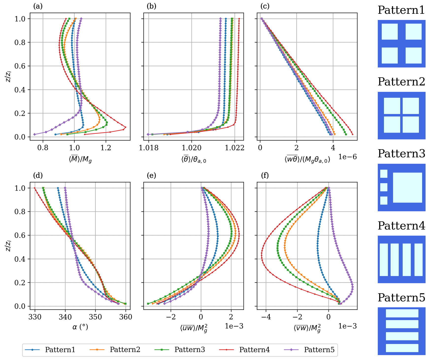
Figure 4 Normalized vertical profiles of (a) horizontal wind speed, (b) potential air temperature, (c) total heat flux, (d) geostrophic wind direction (α), (e) total stress in the streamwise direction, and (f) total stress in the cross-stream direction for all five patterns.

In all five simulations, the largest difference occurs between Pattern4 and Pattern5 (red and purple lines, respectively), which is expected since the geostrophic wind, and thus the near-surface wind, flows parallel (rather than perpendicular) to the strips of ice (Willingham et al., 2014; Anderson et al., 2015; Salesky et al., 2022; Fogarty and Bou-Zeid, 2023a). Although wind direction is not a surface property of sea ice, its orientation relative to the surface features is still an important driver that must be taken into consideration and will be discussed further. All patterns developed a low-level jet (LLJ), which can be seen in Fig. 4a, although the LLJs in Pattern1 and Pattern5 are weak (Tetzlaff et al., 2015; Michaelis et al., 2021). The LLJs seem to strengthen in Pattern2 and Pattern3, likely due to large swaths of ice aligned with the direction of the geostrophic wind; the unstable–stable transitions in these ice regions decouple the air from the surface friction over long, stable ice patches, allowing for low-level wind acceleration. This mechanism is similar to the one advanced by Blackadar (1957), which concerned the creation of a low-level jet via inertial oscillation over time as the ABL transitioned to a stable regime at sunset. However, in this case, the oscillation occurs in space, with columns of air advecting from hot to cold surfaces and decoupling from the surface. The second-strongest LLJ is in Pattern3 and is likely caused by the one large ice floe. It persists across all wind directions, and the same can be said for Pattern2. The strongest LLJ, found in Pattern4, is likely reinforced by secondary circulations (not shown), consisting of streamwise-aligned rolls driven by the lateral contrast in surface temperature, and by the fact that the small strips of ocean between the ice floes are not wide enough to interrupt the circulations. However, unlike Pattern2 and Pattern3, Pattern4 is highly anisotropic, meaning that the geostrophic wind direction is more important in this case, as evidenced by the fact that Pattern5 has no LLJ despite being a 90° rotated version of Pattern4.

Each simulation showed an increase in potential temperature of 2.1 %–2.2 %; this warming is consistent with the large ocean fraction in each of the patterns. Despite initializing the air temperature to produce zero fluxes according to the Monin–Obukhov flux models, which assume equilibrium between the air and water above each surface grid cell, the upward fluxes over warm water are larger than the downward fluxes over cooler ice. This is due to the effect of advection, which perturbs the equilibrium.

Major differences are also observed in the total streamwise and cross-stream stresses, displayed in Fig. 4d and e, respectively. Again, Pattern4 and Pattern5 exhibit the greatest differences from one another due to the geostrophic wind direction. All simulations show similar negative streamwise stress in the surface layer, but at higher altitudes in the MIZ-ABL, the differences between simulations are greater. Above the LLJ, some of the stresses turn positive, implying an upward transfer of momentum from the LLJ, which explains the differences that may be observed below the blending height (Wood and Mason, 1991; Mahrt, 2000; Brunsell et al., 2011). The cross-stream components of the total momentum flux, shown in Fig. 4e, are all quite distinct, indicating significant differences in the Ekman rotation of wind and stress with height.

To further explain the differences seen in these patterns, we consider the decomposition of the total flux into its dispersive and turbulent contributions. Vertical turbulent heat flux is denoted as $\stackrel{\mathrm{‾}}{w^{\prime }{\mathit{\theta }}^{\prime }}$, while vertical turbulent streamwise and cross-stream stresses are denoted as $\stackrel{\mathrm{‾}}{u^{\prime }{w}^{\prime }}$ and $\stackrel{\mathrm{‾}}{v^{\prime }{w}^{\prime }}$, respectively. Dispersive fluxes arise from a time-averaged but spatially variable mean flow (Raupach and Shaw, 1982; Li and Bou-Zeid, 2019). Since our Reynolds averaging is performed over time, we can spatially decompose any Reynolds-averaged variable. For example, the vertical velocity can be decomposed as follows: $\stackrel{\mathrm{‾}}{w}=\langle \stackrel{\mathrm{‾}}{w}\rangle +{\stackrel{\mathrm{‾}}{w}}^{\prime \prime }$, where the brackets represent spatial averaging (as defined in Sect. 2.1) and the double prime represents variations in the mean planar fields in space. We then calculate the local dispersive fluxes, using vertical heat flux as an example, as follows:

$$\begin{array}{}\text{(4)}& {\displaystyle }\stackrel{\mathrm{‾}}{w}\stackrel{\mathrm{‾}}{\mathit{\theta }}& {\displaystyle }=(\langle \stackrel{\mathrm{‾}}{w}\rangle +{\stackrel{\mathrm{‾}}{w}}^{\prime \prime })(\langle \stackrel{\mathrm{‾}}{\mathit{\theta }}\rangle +{\stackrel{\mathrm{‾}}{\mathit{\theta }}}^{\prime \prime })\text{(5)}& {\displaystyle }& {\displaystyle }=\langle \stackrel{\mathrm{‾}}{w}\rangle \langle \stackrel{\mathrm{‾}}{\mathit{\theta }}\rangle +{\stackrel{\mathrm{‾}}{w}}^{\prime \prime }\langle \stackrel{\mathrm{‾}}{\mathit{\theta }}\rangle +\langle \stackrel{\mathrm{‾}}{w}\rangle {\stackrel{\mathrm{‾}}{\mathit{\theta }}}^{\prime \prime }+{\stackrel{\mathrm{‾}}{w}}^{\prime \prime }{\stackrel{\mathrm{‾}}{\mathit{\theta }}}^{\prime \prime }.\end{array}$$

We then spatially average the entirety of Eq. (5) over the horizontal plane to obtain

$$\begin{array}{}\text{(6)}& \langle \stackrel{\mathrm{‾}}{w}\stackrel{\mathrm{‾}}{\mathit{\theta }}\rangle =\langle {\stackrel{\mathrm{‾}}{w}}^{\prime \prime }{\stackrel{\mathrm{‾}}{\mathit{\theta }}}^{\prime \prime }\rangle .\end{array}$$

The middle two terms in Eq. (5) are zero due to spatial averaging, since $\langle {\stackrel{\mathrm{‾}}{w}}^{\prime \prime }\rangle =\mathrm{0}$ and $\langle {\stackrel{\mathrm{‾}}{\mathit{\theta }}}^{\prime \prime }\rangle =\mathrm{0}$ by definition; therefore, these terms have no impact on spatially averaged surface–atmosphere exchanges. Furthermore, $\langle \stackrel{\mathrm{‾}}{w}\rangle$ is assumed to be very small (unless strong, large-scale subsidence or uplift is present). In our LES, $\langle \stackrel{\mathrm{‾}}{w}\rangle$ must be zero since there cannot be accumulation or depletion of mass below a given horizontal plane in a periodic domain with an incompressible flow. Thus, the first term on the right-hand side of Eq. (5) is also negligible, leaving only one term remaining in Eq. (6). This term, denoting dispersive flux, is of particular interest as it represents the coherent spatial correlation of vertical velocity and potential temperature in regions with consistent secondary structures, such as consistently warm updrafts, cool downdrafts, or streamwise rolls.

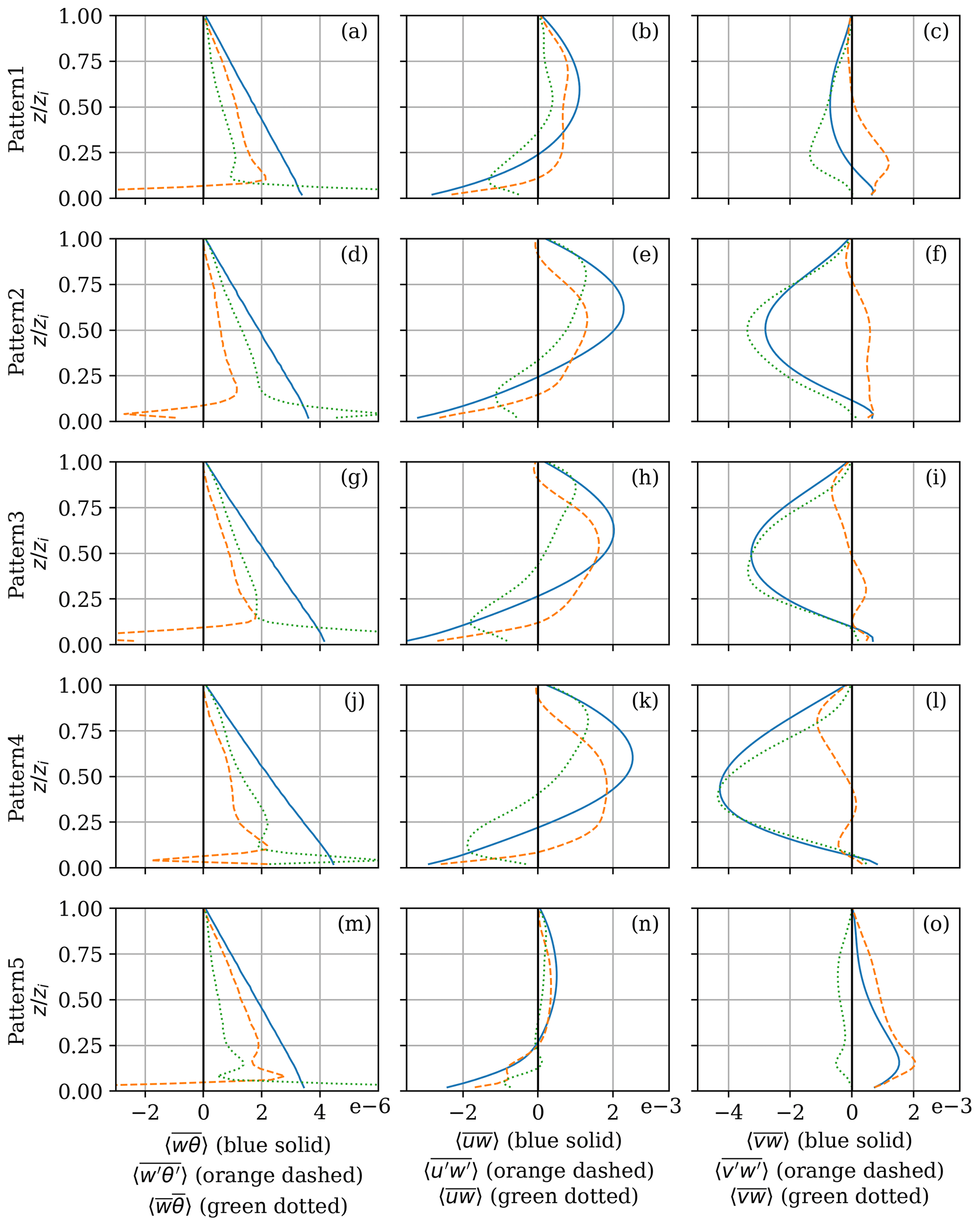
Figure 5 (a, d, g, j, m) Normalized vertical profiles of total heat flux ($\stackrel{\mathrm{‾}}{w\mathit{\theta }}$; solid blue line), turbulent heat flux ($\stackrel{\mathrm{‾}}{w^{\prime }{\mathit{\theta }}^{\prime }}$; dashed orange line), and dispersive heat flux ($\stackrel{\mathrm{‾}}{w}\stackrel{\mathrm{‾}}{\mathit{\theta }}$; dotted green line) for each pattern (as shown in Fig. 4). (b, e, h, k, n) Same as in panels (a), (d), (g), (j), and (m) but for normalized total streamwise stress ($\stackrel{\mathrm{‾}}{uw}$; solid blue line), turbulent streamwise stress ($\stackrel{\mathrm{‾}}{u^{\prime }{w}^{\prime }}$; dashed orange line), and dispersive streamwise stress ($\overline{u}\overline{w}$; dotted green line). (c, f, i, l, o) Same as in panels (a), (d), (g), (j), and (m) but for normalized total cross-stream stress ($\stackrel{\mathrm{‾}}{vw}$; solid blue line), turbulent cross-stream stress ($\stackrel{\mathrm{‾}}{v^{\prime }{w}^{\prime }}$; dashed orange line), and dispersive cross-stream stress ($\overline{v}\overline{w}$; dotted green line).

Figure 5 shows the horizontally averaged vertical profiles of the total, turbulent, and dispersive fluxes of each pattern with respect to heat flux, streamwise momentum flux, and cross-stream momentum flux, allowing us to decompose and analyze the total fluxes shown in Fig. 4c–e. For example, it is clearer now that the cross-stream components of the total momentum flux (Fig. 4e) are distinct from one another due to these dispersive fluxes (dotted green lines). Over these heterogeneous surfaces, dispersive cross-stream stress dominates over its turbulent counterpart in all patterns except Pattern5 (see panels c, f, i, and l in Fig. 5). The magnitudes of these dispersive fluxes are not equal when the heterogeneous surfaces differ from one another. Thus, it is not the ice fraction or average floe area but the surface pattern itself that leads to these differences in total cross-stream flux. The streamwise stresses, on the other hand, seem to balance the dispersive and turbulent stresses, which are not always of the same sign (panels e, h, k, and n in Fig. 5). Thus, the dispersive components that directly result from the secondary motions imprinted by the surface pattern on the atmosphere are also critical here. These secondary circulations can be seen in the two-dimensional cross sections in the supporting information.

The total heat flux in all these simulations linearly decreases with height, as dictated by the LES setup. As seen in Fig. 4c, the variations are not as impressive as those concerning the momentum fluxes, but they can still result in a difference of up to 30 %, especially near the surface. However, analyzing the left column of Fig. 5 (i.e., panels a, d, g, j, and m) shows that the relative importance and profiles of the dispersive and turbulent heat fluxes exhibit more significant differences. The various surface patterns seem to lead to differences in the dispersive fluxes, but in all cases, these are balanced out by the turbulent fluxes. Nevertheless, in all of the figures, there is strong variability near the surface in the dispersive-flux and turbulent-flux profiles. This is partially due to the shallow internal boundary layers that are created by the mean flow and the secondary circulations over the floes, and these differing secondary circulations arise from differences in the surface patterns. However, one should also note that the first few points are strongly influenced by the transition from the wall model to the SGS model in representations of resolved turbulence – a persistent challenge in LESs (Piomelli and Balaras, 2002; Brasseur and Wei, 2010). Thus, the quantitative details of the results from such regions should be interpreted with care.

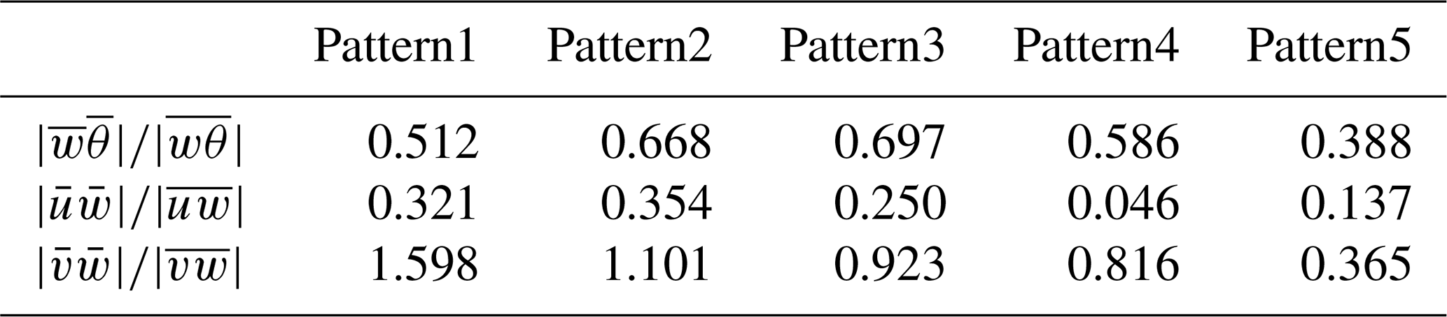
Lastly, analyzing the ratios between dispersive and total atmospheric vertical fluxes (Table 2) provides insight into the differences between simulations and allows for comparisons with other surface types. For example, in Pattern1 and Pattern2, $\left|\overline{v}\overline{w}\right|/\left|\stackrel{\mathrm{‾}}{vw}\right|>\mathrm{1}$, indicating that the dispersive and turbulent fluxes along the cross-stream axis are in opposite directions, as seen in the green and orange profiles in Fig. 5c and f. The ratios in Pattern4 and Pattern5 are also closer to unity than the other values, which, again, highlights the differences in secondary circulations due to the sea ice pattern. These values have been observed before – for example, over urban or forest canopies (Moltchanov et al., 2015; Boudreault et al., 2017; Li and Bou-Zeid, 2019).

Overall, these LES results indisputably indicate that ice–water patterns hold key information on how the MIZ-ABL interacts with the underlying surface; thus, the rest of the paper is dedicated to characterizing these patterns.

Table 2 Ratios between dispersive and total atmospheric vertical fluxes.

4 Results: statistical analysis

Now that we have established the need for surface characteristics beyond sea ice fraction, we aim to examine the indicators that can be used for this purpose. For each of the nine resolutions considered, 44 observed sea ice images were analyzed. When conducting this analysis at the 2 m resolution, four metrics (including sea ice fraction) remained after the VIF elimination process and did not exhibit multicollinearity with one another: sea ice fraction (f_i), patch density (PD), the splitting index (SPLIT), and the perimeter–area fractal dimension (PAFRAC). These remaining metrics were then categorized into the different metric groups defined in Sect. 2.3: sea ice fraction is an Area and Edge metric, PD and SPLIT are both Aggregation metrics, and PAFRAC is a Shape metric. No metrics remained in the Diversity, Core Area, or Contrast metric groups. We expected no metrics to remain in the Contrast metric group since an edge can only exhibit one contrast for a sea-ice–water surface – however, this could change if the analysis were conducted with continuously variable surface temperatures or roughness lengths. We also did not expect any metrics from the Diversity group since many metrics, such as evenness or Simpson's diversity index, are functions of sea ice fraction. The absence of metrics from the Core Area group was not predicted, but it is likely related to the fact that the Shape group and the Area and Edge group can collectively represent the Core Area characteristics.

The first aggregation metric, PD (Riitters et al., 1995; Šímová and Gdulová, 2012), with a VIF of 1.9, represents an area-normalized number of patches and is described as follows:

$$\begin{array}{}\text{(7)}& \text{PD}={\displaystyle \frac{n}{A_{\mathrm{t}}}},\end{array}$$

where PD represents patch density, A_t represents the total area of the surface, and n represents the total number of distinct patches (of either sea ice or water). As the PD of a sea ice surface increases, one would expect to find more instances of ice–water edges and thus more regions of stable-to-unstable and unstable-to-stable stratification transitions. We also note that reducing PD increases the average time a parcel spends over the stable (or unstable) surface, which affects how the parcel adjusts to the transition to a new stability regime. Patch density may also work in tandem with geostrophic wind direction, as discussed in Sect. 3, since geostrophic wind flowing in one direction may encounter more ice–water-edge transitions than in another direction (see Pattern4 and Pattern5, for example).

The second metric, SPLIT, with a VIF of 1.9, was first described in Jaeger (2000). It represents the inverse probability that two randomly chosen points on a map will be in the same patch, and the corresponding equation is expressed as follows:

$$\begin{array}{}\text{(8)}& \text{SPLIT}={\displaystyle \frac{A_{\mathrm{t}}^{\mathrm{2}}}{{\sum }_{i=\mathrm{1}}^n{a}_i^{\mathrm{2}}}},\end{array}$$

where a_i is the area of patch i and the index (i) iterates over all patches. SPLIT has a value of n if there is only one patch or if all patches are of an equal size. However, generally, SPLIT has a value greater than n, with lower values indicating a larger variance in patch sizes. Since we already use PD, the new information provided by SPLIT is specifically about the variance in patch sizes.

The only Shape metric, PAFRAC, with a VIF of 2.1, is obtained by regressing each patch's perimeter (P_i) against its area (A_i) on a log–log plot, resulting in the following:

$$\begin{array}{}\text{(9)}& A=k{P}^{\mathrm{2}/\mathrm{PAFRAC}},\end{array}$$

where k is a constant and PAFRAC is the perimeter–area fractal dimension, which measures the tortuosity, or jaggedness, of an ice–water interface, similar to any fractal dimension (Mandelbrot, 1982).

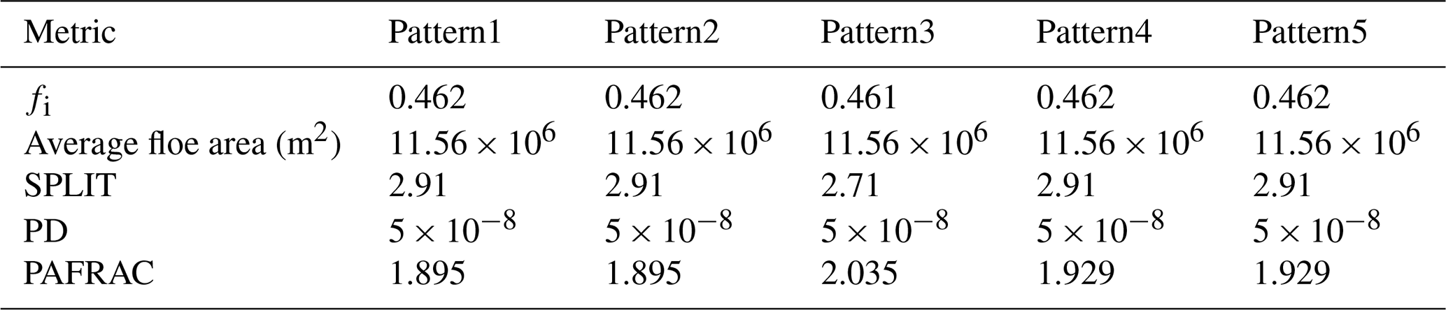
Thus, in addition to sea ice fraction (f_i), the three metrics that would be useful in describing a sea ice surface are SPLIT, PD, and PAFRAC. Table 3 details the values of these metrics for each of the sea ice patterns simulated in Sect. 3. We observe that SPLIT is invariant to the shape of the floes as long as the areas of the floes are equivalent (i.e., no variance), which is why SPLIT remains consistent for all patterns except Pattern3. This is where PAFRAC proves useful as it provides three different values among the five ice–water patterns.

Table 3 Landscape metrics of the simulations conducted in Sect. 3. Note that for maps with a low number of patches (fewer than 10) and/or simple shapes, the PAFRAC metric may exceed the theoretical range, as observed in Pattern3. However, this does not appear in any of the real sea ice maps we examine next.

For the real ice maps obtained from Arctic images, the ice fraction varies from 0.19 to 0.99, PD varies from 5.4 to 42.5, SPLIT varies from 1.23 to 4.07, and PAFRAC varies from 1.338 to 1.726 at a 2 m map resolution. In many cases, however, numerical simulations also require the resampling of high-resolution surfaces by increasing the grain (pixel) size. For example, sea ice maps from reconnaissance satellites may have a resolution of up to 1 m, but this is computationally impractical for numerical weather models. Large-eddy simulations of the ABL can have resolutions down to 50 m, while NWP models have resolutions of 2 to 10 km. Therefore, even with high-resolution data, the aggregation and resampling of these surface patterns are inevitable in modeling. Furthermore, considering the operational use of these metrics, regularly updating these values would likely involve multiple satellite products with differing resolutions; thus, metrics that can be extrapolated/interpolated across different grid cell sizes would allow for consistent computation when standardized to a single weather model grid cell.

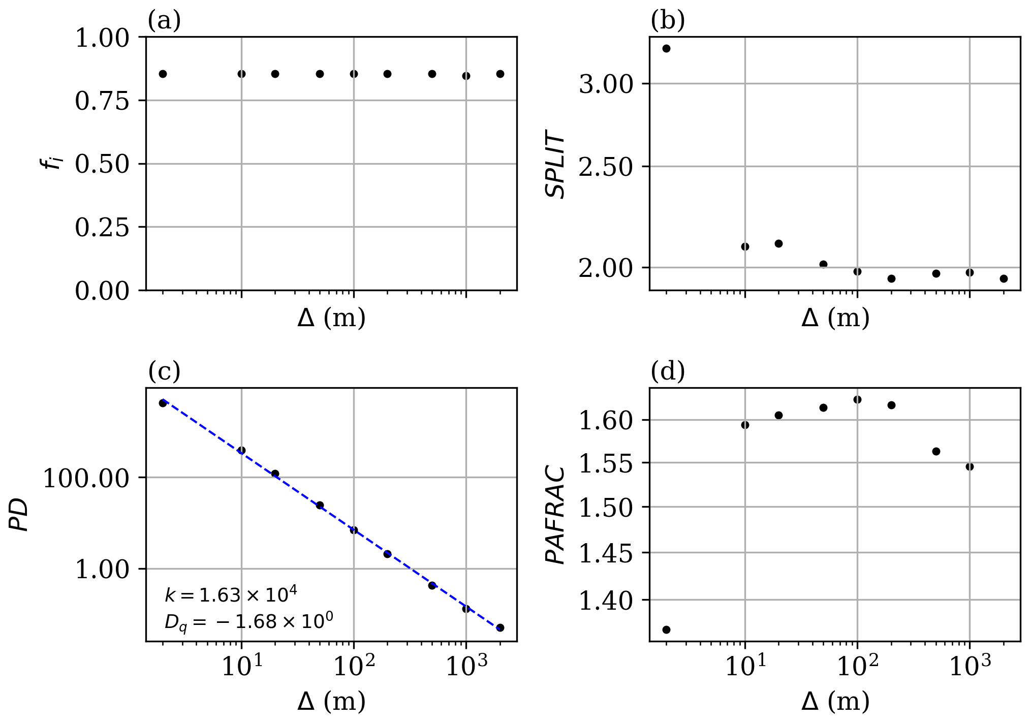
Figure 6 Landscape metrics plotted against resolution with respect to (a) sea ice fraction, (b) the splitting index, (c) patch density, and (d) the fractal dimension. A power law of the form $m=k{\mathrm{\Delta }}^{D_q}$ is fitted to the patch density plot (dashed blue line), but no such power law applies to the other three metrics.

Therefore, it is useful to examine how these chosen metrics vary as an image is aggregated to a resolution applicable to numerical weather models (or other numerical models, such as LESs); an appealing metric would be one that is invariant to resolution changes. Sea ice fraction (f_i) is a good example of an invariant indicator, as shown in Fig. 6a, where it is calculated for all images and then averaged over the corresponding resolution. A second-best case would involve a metric that exhibits a clear scaling law relative to the resolution, such as the PD depicted in Fig. 6b. In this case, the PD for the “real” 2 m resolution surface can be extrapolated to higher resolutions based on power-law scaling, expressed as

$$\begin{array}{}\text{(10)}& m=k{\mathrm{\Delta }}^{D_q},\end{array}$$

where m is the metric, Δ is the map resolution, and k and D_q are the scaling coefficients.

Some metrics, such as SPLIT and PAFRAC, seem to exhibit near-invariant behavior after a certain jump in the resolution. For example, when starting from the 10 m resolution, SPLIT stays fairly constant as the resolution decreases. There is also variation in PAFRAC as the resolution decreases from 10 m. This is consistent with results from previous studies as some landscape metrics exhibit large errors when surfaces are aggregated to lower resolutions (Moody and Woodcock, 1994, 1995). Given the near-invariant scaling of three of the four metrics and the predictable power-law scaling of the fourth, we can proceed with these four metrics since they are usable (or translatable) across scales.

5 Principal direction of the sea ice patterns

Thus far, we have identified four surface pattern indicators that characterize the MIZ surface: sea ice versus water concentration (f_i), patch density (PD), variance in the sizes of patches (SPLIT), and the tortuosity of patch edges (PAFRAC). However re-examining Pattern4 and Pattern5 in Fig. 4 raises the question of why these maps show the largest differences in their respective MIZ-ABLs. Although their geometric patterns are the same (and thus the four metrics are identical for the two configurations), the difference in the geostrophic wind direction results in large differences in the surface–atmosphere interactions. This suggests that another important attribute relates to how the surface patterns are oriented relative to the wind. If the surface is isotropic, the wind angle should be irrelevant, but most water–sea-ice patterns in the MIZ display a significant degree of anisotropy (Feltham, 2008). Therefore, quantifying the impact of surface orientation and including it in the set of metrics obtained from the VIF analysis, as discussed in Sect. 4, may provide additional information, allowing modelers to parameterize MIZ-ABL dynamics in global climate models.

We observe that in Pattern4 and Pattern5, the difference in geostrophic direction is related to the directionality of sea ice organization. In Pattern4, the wind blows consistently over an infinitely repeating pattern of sea ice and water at regular intervals. In Pattern5, the wind blows over much longer strips of ice and water, even though some sea-ice–water transitions are present. Any other oblique flow is thus in between these two parallel and perpendicular regimes. We characterize the differences between these regimes by examining the variance in the surface exposed to the wind. In other words, Pattern4 exhibits high variance since the surface wind flows over a maximum of eight ice–water transitions within one domain length, whereas Pattern5 exhibits low variance since the wind flows over a maximum of two sea-ice–water transitions. This then raises the question of how to determine a principal direction for a more complex surface.

We therefore attempted to characterize this anisotropy by computing the direction of the eigenvector (the eigendirection) for the surface with the least amount of variance, resulting in the fewest ice–water transitions possible. This was done using the scikit-learn Python package, specifically via principal component analysis (PCA) using the sklearn.decomposition.PCA class (Pedregosa et al., 2011). This method performs an eigendecomposition of the covariance matrix of the sea ice map, yielding two orthogonal eigenvectors. The principal eigendirection points in the direction of minimal variance, as indicated by the longer of the two arrows in Fig. 7. In other words, the principle or most coherent mode that best explains the pattern is aligned with the direction of least variability. The secondary eigendirection is, by definition, orthogonal to the principal eigenvector. Some of these eigendirections are intuitive as one can imagine trying to select a geostrophic wind direction that passes over a minimal number of ice–water edges. The maps in Figs. 7a and 7g provide two such examples. However, the map in Fig. 7f, for example, is a bit less intuitive – visual inspection may suggest that the principle eigendirection should be aligned from the lower-right corner of the map to the upper-left corner, but the results indicate a less obvious orientation.

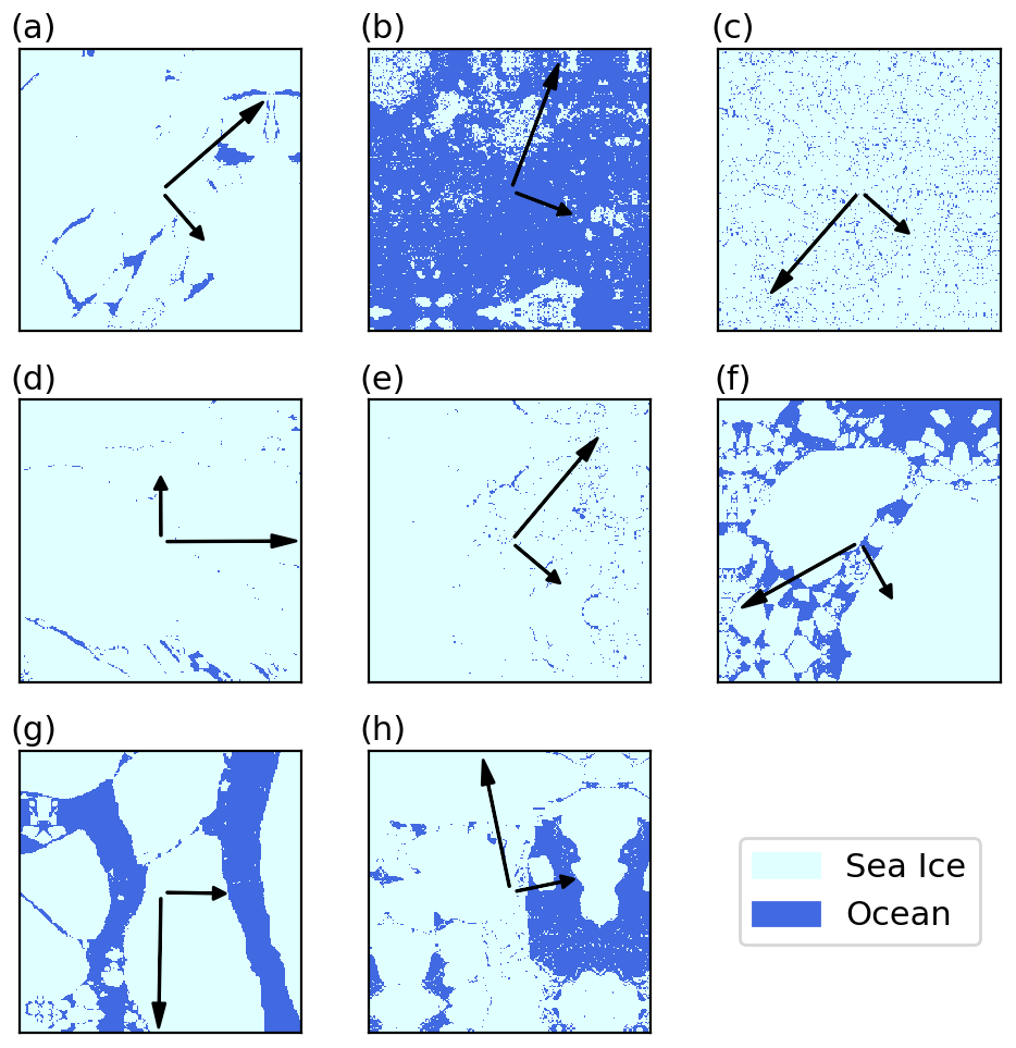
Figure 7 Eight maps from the sea ice dataset, each overlaid with their principal eigendirection (long arrow) and secondary eigendirection (short arrow), computed via principal component analysis.

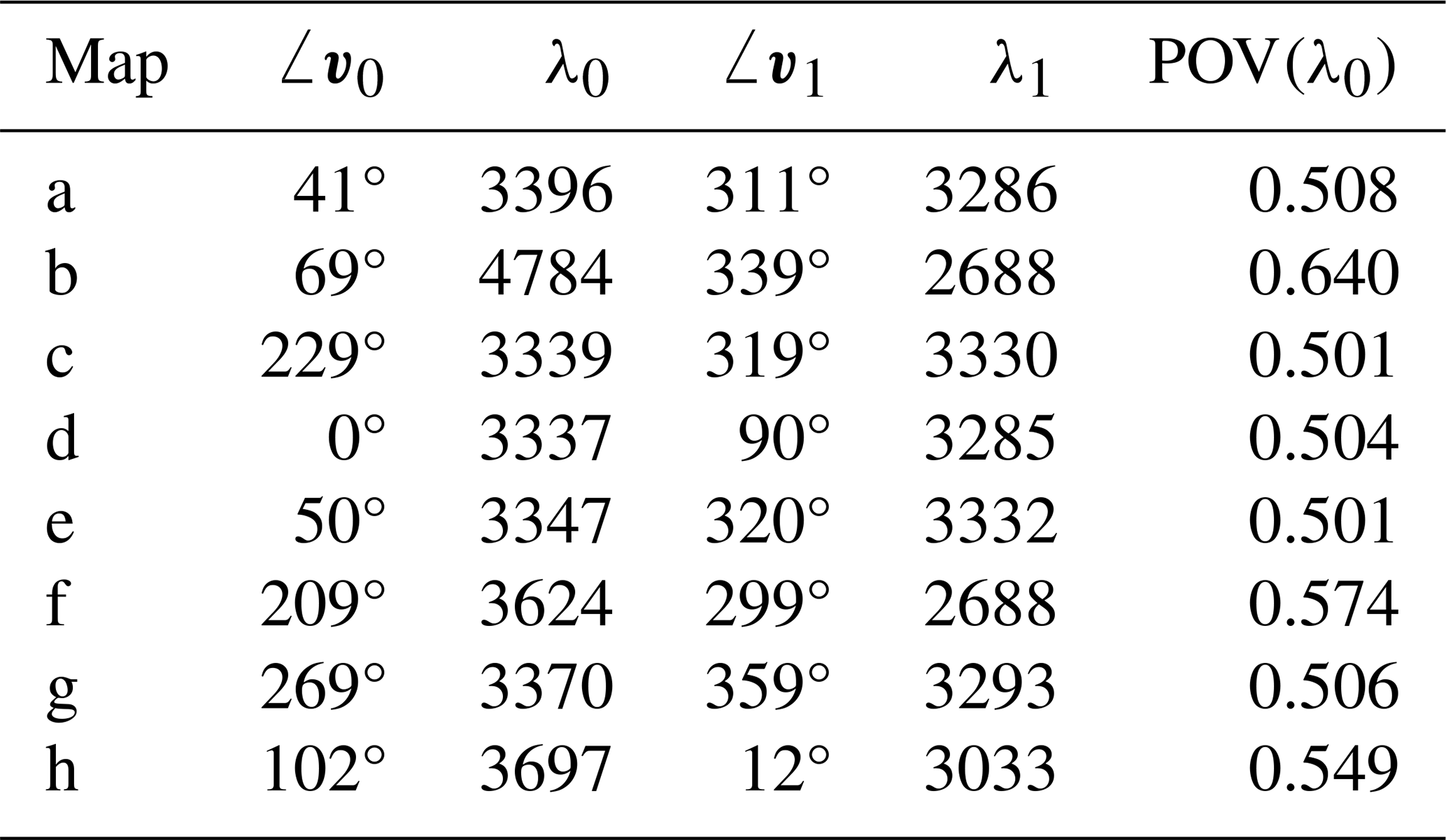
Table 4 Eigenvector (v_i) angles and eigenvalues (λ_i) for principal eigenvectors (i=0) and secondary eigenvectors (i=1), as well as the percentage of variance (POV) of λ₀, corresponding to each map (Fig. 7a–h). Note that these angles are not traditional meteorological wind angles but are instead given in Cartesian coordinates; 0° represents a left-to-right westerly wind, and 90° represents a southerly wind.

It is hypothesized that, for a fixed sea ice fraction (f_i), geostrophic wind flowing in the principal direction with minimal variance will behave more like Pattern5, while the perpendicular angle to said principal direction (the secondary direction) will behave more like Pattern4 – similar to the parallel and perpendicular cases in the simulations conducted in Fogarty and Bou-Zeid (2023a). Nevertheless, further LESs are needed to elucidate the exact impact of this relative orientation and the other parameters we identified on the MIZ-ABL.

However, some of these maps exhibit a higher degree of anisotropy than others, such as Fig. 7c. To measure the degree of anisotropy in these maps, one can look at the percentage of variance (POV), defined as

$$\begin{array}{}\text{(11)}& \text{POV}\left({\mathit{\lambda }}_i\right)={\displaystyle \frac{{\mathit{\lambda }}_i}{{\sum }_{i=\mathrm{0}}^n{\mathit{\lambda }}_i}},\end{array}$$

where λ_i is an eigenvalue in an n-dimensional matrix. The POV for a two-dimensional surface (n=2) thus describes the amount of variance that can be explained (or reconstructed) by that eigenvector alone, resulting in the following relationship: $\text{POV}\left({\mathit{\lambda }}_{\mathrm{0}}\right)+\text{POV}\left({\mathit{\lambda }}_{\mathrm{1}}\right)=\mathrm{1}$. In theory, a sea ice map with a high POV(λ₀) value, and thus a low POV(λ₁) value, would be anisotropic since the secondary eigendirection would account for much more of the variance than the principal eigendirection, and the surface would thus have a preferential direction of variability (one would expect Fig. 7g to have a high POV(λ₀) value). Conversely, a map with a low POV(λ₀) value would be fairly isotropic.

By definition, POV(λ₀)≥0.5 (where $\text{POV}\left({\mathit{\lambda }}_{\mathrm{0}}\right)=\text{POV}\left({\mathit{\lambda }}_{\mathrm{1}}\right)=\mathrm{0.5}$ indicates a truly isotropic surface) since POV(λ₀) represents the POV for the principal eigendirection. However, most of the ratios in these examples lie in the range of $\mathrm{0.50}<\text{POV}\left({\mathit{\lambda }}_{\mathrm{0}}\right)<\mathrm{0.60}$, showing little variability among these maps. Thus, in this small subset of sea ice maps, examining only POV(λ₀) would not provide information on how much influence the principal eigendirection has.

6 Conclusions

Although stability over an ice- or water-dominated surface depends on many factors, such as wind direction and potential air temperature, in the cases where potential air temperature falls between the surface temperatures of ice and water, the ice fraction of a sea ice surface can be a fair indicator of the behavior of the MIZ-ABL. However, this is only the case when the ice fraction approaches 0.0 (all ocean), leading to an unstable atmosphere, or 1.0 (all ice), leading to a stable atmosphere. On the other hand, when f_i falls between these limits (in other words, when the surface flow alternates between very stable and very unstable), the ice fraction alone is insufficient to predict the dynamics and thermodynamics of the MIZ-ABL. Large-eddy simulations conducted for five different sea ice surfaces, as detailed in Fig. 2, have shown that surfaces with the same ice fraction, number of floes, and mean floe size can result in very distinct atmospheric dynamics. Differences were observed in horizontal wind speed (Fig. 4a) and total surface stresses (Figs. 4d–e and 5).

While Fig. 5 shows moderate differences in the total heat flux, which, in this case, is constrained by the simulation setup, more significant differences are observed in the dispersive and turbulent fluxes that make up this total flux (see also Table 2). The total, turbulent, and dispersive fluxes of the streamwise and cross-stream momenta are even more sensitive to surface patterns. These dispersive fluxes have been shown to drive many of the differences and are thus non-negligible in climate models (Margairaz et al., 2020; Fogarty and Bou-Zeid, 2023a; Lu et al., 2023).

To understand what other information can be obtained from a two-dimensional, binary lattice surface, we examined 44 spatial metrics traditionally used in the field of landscape ecology since knowing the cover fraction (ice fraction) and the number and median area of the floes is not enough to able to fully describe the ice–water–atmosphere physics. These 44 additional spatial metrics were applied to LIDPs of real-world satellite sea ice imagery to determine which metrics were important, and the variance inflation factor was used to detect and remove any multicollinearity in this dataset. The remaining metric set included the following metrics: ice fraction, patch density (representing the number of sea ice floes and, thus, their mean size in a given area), the splitting index (representing variance in floe sizes), and the perimeter–area fractal dimension (representing edge tortuosity). We also proposed using the surface eigendirection relative to the mean wind direction to characterize the influence of surface anisotropy and its interaction with the wind direction.

The resulting set of five metrics, including eigendirection, is useful for describing a two-dimensional surface. However, based on the VIF analysis, it also represents a minimal set of indicators needed to describe such a surface since these metrics contain distinct and important information. Nevertheless, the development of practical parameterizations for sea ice and the MIZ-ABL will ultimately need to include additional considerations, including the ease of obtaining these parameters for modeling applications, the computing time needed to calculate these surface metrics dynamically versus that needed to resolve surface features when running an ESM, and the availability of easier-to-compute surrogate metrics.

The first step in answering this broad question is to investigate to what degree these other metrics affect the MIZ-ABL compared to the first-order effect of ice fraction on the MIZ-ABL. In other words, given a specific ice fraction, how will changing any of the metrics in the resulting set affect the overlying MIZ-ABL? While this study addressed this question for idealized surfaces and established the relevance of these parameters under certain conditions, determining which parameters will be critical for real ice maps – and understanding their frequency and impact – requires additional simulations, and a follow-up to this study is underway (see Fogarty et al., 2024). More turbulence-resolving numerical simulations of real ice surfaces are thus needed.

Another crucial step in answering this question involves figuring out how one would go about creating an accurate parameterization based on available external grid cell variables; the resources needed to answer this question may be extensive, especially considering that, in this age of machine learning, high-resolution synthetic satellite imagery is generated more frequently (see Au-Boehm et al., 2024). Even more large-eddy simulations over real sea ice maps, beyond what has been discussed here, are imperative for answering this question. Lastly, this open question also requires us to look at how to incorporate the resulting metrics and eigendirections into these climate models. This includes examining (i) how the geostrophic wind (at certain principal directions) interacts with the resulting metric set, (ii) other possible metrics of anisotropy, and (iii) how a sea ice model in an ESM can provide the data needed to capture the heterogeneity of the sea ice surface, as well as other questions that remain unanswered at this time.

Appendix A: Details of the large-eddy simulation

In this study, incompressible filtered Navier–Stokes equations (along with a Boussinesq approximation for the mean state) and a heat budget are solved for a horizontally periodic flow, where a variable with a tilde represents a quantity filtered via the numerical grid spacing (Δ). The equations are expressed as follows:

$$\begin{array}{}\text{(A1)}& {\displaystyle \frac{\partial {\stackrel{\mathrm{̃}}{u}}_i}{\partial x_i}}=\mathrm{0},\text{(A2)}& {\displaystyle }\begin{array}{rl}{\displaystyle \frac{\partial {\stackrel{\mathrm{̃}}{u}}_i}{\partial t}}+{\stackrel{\mathrm{̃}}{u}}_j{\displaystyle \frac{\partial {\stackrel{\mathrm{̃}}{u}}_i}{\partial x_j}}& =-{\displaystyle \frac{\mathrm{1}}{{\mathit{\rho }}_{\mathrm{r}}}}{\displaystyle \frac{\partial p}{\partial x_j}}+{\stackrel{\mathrm{̃}}{F}}_i+f_{\mathrm{c}}{\mathit{ϵ}}_{ij\mathrm{3}}{\stackrel{\mathrm{̃}}{u}}_j\\ & -g{\mathit{\delta }}_{i\mathrm{3}}(\mathrm{1}-{\displaystyle \frac{\widehat{\mathit{\theta }}}{{\mathit{\theta }}_{\mathrm{r}}}})-{\displaystyle \frac{\partial {\mathit{\tau }}_{ij}}{\partial x_j}},\end{array}\text{(A3)}& {\displaystyle \frac{\partial \stackrel{\mathrm{̃}}{\mathit{\theta }}}{\partial t}}+{\stackrel{\mathrm{̃}}{u}}_j{\displaystyle \frac{\partial \stackrel{\mathrm{̃}}{\mathit{\theta }}}{\partial x_j}}=-{\displaystyle \frac{\partial q_j}{\partial x_j}}.\end{array}$$

The equations above use the Einstein summation rule, where i represents the free index and j represents the repeated index. Moreover, u_i represents the velocity vector; x_i represents the position vector; p represents modified pressure (see Bou-Zeid et al., 2005, for details); θ represents the potential temperature;θ_r and $\widehat{\mathit{\theta }}$ represent the Boussinesq reference (the planar mean in our calculations) and the perturbation from said reference for potential temperature, respectively; ρ_r represents the reference mean density corresponding to θ_r; and F_i represents the main flow-driving force (a synoptic pressure gradient). The Coriolis force is represented by the third term on the right-hand side of Eq. (A2), where f_c is the Coriolis parameter and ϵ_ij3 represents the Levi-Civita symbol. Buoyancy is represented by the fourth term on the right-hand side of Eq. (A2), where δ_ij represents the Kronecker delta.

An overbar denotes averaging over time, which is used as a surrogate for ensemble Reynolds averaging, while spatial averaging over the heterogeneous domain (in both x and y) is denoted by angle brackets. The subgrid-scale stress (${\mathit{\tau }}_{ij}=\stackrel{\mathrm{̃}}{u_i{u}_j}-{\stackrel{\mathrm{̃}}{u}}_i{\stackrel{\mathrm{̃}}{u}}_j$) and buoyancy flux ($q_j=\stackrel{\mathrm{̃}}{u_j\mathit{\theta }}-{\stackrel{\mathrm{̃}}{u}}_j\stackrel{\mathrm{̃}}{\mathit{\theta }}$), which result from the filtering, are modeled using a scale-dependent Lagrangian dynamic model (Bou-Zeid et al., 2005) with a constant subgrid-scale Prandtl number (Pr) of 0.4. As noted before, the numerical grid serves as the inherent filter of the model, but any explicit filtering needed to compute the dynamic Smagorinsky constant (c_s) is done at scales of 2Δ and 4Δ (2Δ for the local wall model); for these computations, a sharp spectral cutoff filter is used. This model was validated by Bou-Zeid et al. (2005) for boundary layer flows over both homogeneous and heterogeneous terrain by reproducing experimental velocity and stress profiles obtained by Bradley (1968) following a change in surface roughness. It was further validated for urban flows (Tseng et al., 2006; Li et al., 2016), as well as for both stable and unstable boundary layers (Kleissl et al., 2006; Kumar et al., 2006; Huang and Bou-Zeid, 2013). Therefore, the ability of this model to successfully capture the impacts of stability and spatial transitions in surface properties was not tested further in this paper.

The LES employs boundary conditions that are periodic in the horizontal direction, with zero vertical velocity at the top and bottom of the domain, as well as a stress-free top lid (${\partial }_z{u}_i=\mathrm{0}$, where $i=\mathrm{1},\mathrm{2}$) with zero heat flux. These conditions mimic a very strong top inversion and are adequate for our setup since the top of the domain is not stably stratified, eliminating the need for a sponge layer that prevents wave reflection. This allows for the surface characteristics to be isolated from z_i and the inversion strength. The indices ($i=\mathrm{1},\mathrm{2},\mathrm{3}$) represent the x, y, and z directions, oriented along the streamwise, cross-stream, and vertical directions, respectively. At the bottom of the domain, the surface stress and heat flux are computed by a wall model based on a local law-of-the-wall formulation (Bou-Zeid et al., 2005), incorporating a Monin–Obukhov buoyancy correction. Numerically, a pseudo-spectral approach is employed in the horizontal direction, and an explicit second-order centered-difference scheme is used in the vertical direction. Time advancement is carried out using the fully explicit second-order Adams–Bashforth scheme. Dealiasing of the convective terms is performed using the “$\mathrm{3}/\mathrm{2}$ rule” (Orszag, 1971). Pressure is computed from a Poisson equation obtained by taking the divergence of the momentum equation and applying the incompressibility assumption.

Appendix B: Temperature initialization

The initial potential temperature was chosen so that the mean heat flux over the entire domain was zero; in other words, the heat flux going into the ice was equal in magnitude to the heat flux coming from the water, based on the area fraction of the domain (in this case, the ice fraction). Thus, the initial potential air temperature of the large-eddy simulation was chosen to ensure that the ice-fraction-weighted heat flux over the ice (f_iH_i) was equivalent to the water-fraction-weighted heat flux over the ocean (f_wH_w), resulting in the following equation:

$$\begin{array}{}\text{(B1)}& -f_{\mathrm{i}}{H}_{\mathrm{i}}=f_{\mathrm{w}}{H}_{\mathrm{w}},\end{array}$$

where $f_{\mathrm{i}}+f_{\mathrm{w}}=\mathrm{1}$. Monin–Obukhov flux profile relations were used to express the surface fluxes as follows:

$$\begin{array}{}\text{(B2)}& {\displaystyle }{\mathit{\theta }}_{\mathrm{i}}-{\mathit{\theta }}_{\mathrm{a}}& {\displaystyle }={\displaystyle \frac{H_{\mathrm{i}}}{\mathit{\kappa }{u}_{*,i}\mathit{\rho }{c}_p}}\left[\ln \right({\displaystyle \frac{z}{z_{\mathrm{0}h,\mathrm{i}}}})-{\mathrm{\Psi }}_{\mathrm{s}}({\displaystyle \frac{z}{L_{\mathrm{i}}}}\left)\right],\text{(B3)}& {\displaystyle }{\mathit{\theta }}_{\mathrm{w}}-{\mathit{\theta }}_{\mathrm{a}}& {\displaystyle }={\displaystyle \frac{H_{\mathrm{w}}}{\mathit{\kappa }{u}_{*,\mathrm{w}}\mathit{\rho }{c}_p}}\left[\ln \right({\displaystyle \frac{z}{z_{\mathrm{0}h,\mathrm{w}}}})-{\mathrm{\Psi }}_{\mathrm{u}}({\displaystyle \frac{z}{L_{\mathrm{w}}}}\left)\right],\end{array}$$

where θ_a represents the bulk potential air temperature; θ_i represents the temperature of the ice surface; θ_w represents the temperature of the ocean surface; κ≈0.4 represents the von Kármán constant; $u_{*,\mathrm{i}}$ and $u_{*,\mathrm{w}}$ represent the friction velocities of the ice and water surfaces, respectively; ρ represents the density of air; c_p represents the specific heat of air; z represents the height near the surface (taken at z=50 m); z_0h,i and z_0h,w represent the scalar roughness lengths of the ice and water surfaces, respectively; L_i and L_w represent the Obukhov lengths over the ice and water surfaces, respectively; and Ψ_s and Ψ_u represent the stable and unstable correction functions, respectively, as described in Brutsaert (2005). These Obukhov lengths are defined as

$$\begin{array}{}\text{(B4)}& {\displaystyle }{L}_{\mathrm{i}}& {\displaystyle }={\displaystyle \frac{-u_{*,\mathrm{i}}^{\mathrm{3}}\mathit{\rho }{c}_p}{H_{\mathrm{i}}\mathit{\kappa }(g/{\mathit{\theta }}_{\mathrm{a}})}},\text{(B5)}& {\displaystyle }{L}_{\mathrm{w}}& {\displaystyle }={\displaystyle \frac{-u_{*,\mathrm{w}}^{\mathrm{3}}\mathit{\rho }{c}_p}{H_{\mathrm{w}}\mathit{\kappa }(g/{\mathit{\theta }}_{\mathrm{a}})}},\end{array}$$

where the values of H_i and H_w in these equations are taken as first-order estimates obtained by rearranging Eqs. (B2) and (B3) without the stability functions (i.e., assuming a neutral atmosphere). H_i and H_w are given as

$$\begin{array}{}\text{(B6)}& {\displaystyle }{H}_{\mathrm{i}}& {\displaystyle }=({\mathit{\theta }}_{\mathrm{i}}-{\mathit{\theta }}_{\mathrm{a}})\mathit{\kappa }{u}_{*,\mathrm{i}}(\ln {\displaystyle \frac{z}{z_{\mathrm{0}h,\mathrm{i}}}}{)}^{-\mathrm{1}},\text{(B7)}& {\displaystyle }{H}_{\mathrm{w}}& {\displaystyle }=({\mathit{\theta }}_{\mathrm{w}}-{\mathit{\theta }}_{\mathrm{a}})\mathit{\kappa }{u}_{*,\mathrm{w}}(\ln {\displaystyle \frac{z}{z_{\mathrm{0}h,\mathrm{w}}}}{)}^{-\mathrm{1}}.\end{array}$$

This allows one to derive a function by substituting Eqs. (B2) and (B3) into Eq. (B1), resulting in a function that can be solved for θ_a via a numerical root-finding approach. Of course, this is only a first guess for initializing the LES, which will then dynamically create its potential air temperature field during the warm-up period. As noted in the main text, the actual domain-averaged heat flux in the LES will not be zero.

Appendix C: Landscape quantification metrics

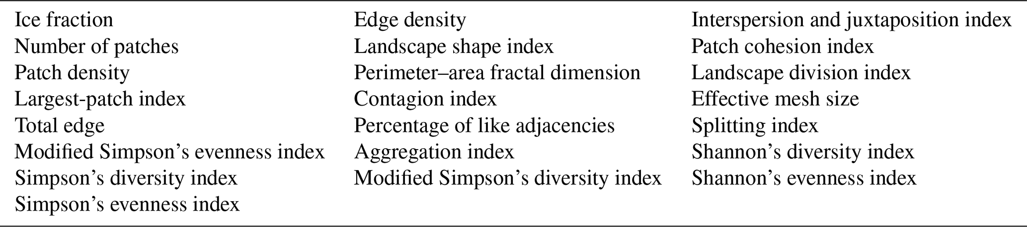
Table C1 lists the landscape metrics used in the VIF analysis conducted in Sect. 4. For more information on each individual metric (apart from ice fraction), consult the FRAGSTATS manual (McGarigal and Marks, 1995).

Table C1 All landscape metrics used in the VIF analysis conducted in Sect. 4.