the Creative Commons Attribution 4.0 License.
the Creative Commons Attribution 4.0 License.
 | 04 Sep 2024
AWI-ICENet1: a convolutional neural network retracker for ice altimetry
Alireza Dehghanpour
Ronny Hänsch
Erik Loebel
Martin Horwath
Angelika Humbert
The Greenland and Antarctic ice sheets are important indicators of climate change and major contributors to sea level rise. Hence, precise, long-term observations of ice mass change are required to assess their contribution to sea level rise. Such observations can be achieved through three different methods. They can be achieved directly by measuring regional changes in the Earth's gravity field using the Gravity Recovery and Climate Experiment Follow-On (GRACE-FO) satellite system. Alternatively, they can be achieved indirectly by measuring changes in ice thickness using satellite altimetry or by estimating changes in the mass budget using a combination of regional climate model data and ice discharge across the grounding line, based on multi-sensor satellite radar observations of ice velocity (Hanna et al., 2013). Satellite radar altimetry has been used to measure elevation change since 1992 through a combination of various missions. In addition to the surface slope and complex topography, it has been shown that one of the most challenging issues concerns spatial and temporal variability in radar pulse penetration into the snowpack. This results in an inaccurate measurement of the true surface elevation and consequently affects surface elevation change (SEC) estimates. To increase the accuracy of surface elevation measurements retrieved by retracking the radar return waveform and thus reduce the uncertainty in the SEC, we developed a deep convolutional-neural-network architecture (AWI-ICENet1). AWI-ICENet1 is trained using a simulated reference data set with 3.8 million waveforms, taking into account different surface slopes, topography, and attenuation. The successfully trained network is finally applied as an AWI-ICENet1 retracker to the full time series of CryoSat-2 Low Resolution Mode (LRM) waveforms over both ice sheets. We compare the AWI-ICENet1-retrieved SEC with estimates from conventional retrackers, including the threshold first-maximum retracker algorithm (TFMRA) and the European Space Agency's (ESA) ICE1 and ICE2 products. Our results show less uncertainty and a great decrease in the effect of time-variable radar penetration, reducing the need for corrections based on its close relationship with backscatter and/or leading-edge width, which are typically used in SEC processing. This technique provides new opportunities to utilize convolutional neural networks in the processing of satellite altimetry data and is thus applicable to historical, recent, and future missions.
- Article
(35911 KB) - Full-text XML
- BibTeX
- EndNote


Ice sheet mass loss is a major contributor to sea level rise. The Greenland Ice Sheet (GrIS) alone contributed 21.0±1.9 mm (Otosaka et al., 2023) between 1992–2022, while Antarctica contributed 7.6±3.9 mm between 1992–2017 (Shepherd et al., 2018). The non-linearity of mass loss from Antarctica is driven by West Antarctica, where glacier acceleration and retreat have caused an increasing contribution since 1992 (Rignot et al., 2002, 2014; Mouginot et al., 2014; Scheuchl et al., 2016; Milillo et al., 2022; Christie et al., 2023). The stability of the West Antarctic Ice Sheet (WAIS) is a major concern (Joughin and Alley, 2011) as even a single glacier, Thwaites Glacier, has the potential to contribute 65 cm to sea level rise (Scambos et al., 2017). This exemplifies the need for accurate observations of ice sheet mass loss. Due to the self-gravitation effect, local sea level rise along the world's coastlines strongly depends on the spatial distribution of ice sheet mass loss (Larour et al., 2017). This is where the advantage of altimeters comes into play. Altimeter data can provide data on ice sheet mass loss at a high spatial resolution compared to gravimeters. The accuracy of altimeter-based mass loss products depends on the precision of the individual elevation measurements, the repeat cycle, the spatial interpolation scheme, and the conversion from volume change to mass change (including firn densification). In this study, we focus on improving the accuracy of individual elevation measurements.
Ku-band satellite altimeters have been surveying ice sheets since the early 1990s with substantial coverage, beginning with ERS-1 and ERS-2 from the ESA, followed by Envisat from 2002–2012. The launch of CryoSat-2 in 2010 marked the introduction of the first altimeter dedicated to studying the Earth's cryosphere. CryoSat-2 orbits at an unusually high inclination, reaching latitudes of 88° N and 88° S. In addition, it includes major improvements for measuring icy surfaces. Alongside the conventional Low Resolution Mode (LRM), a synthetic-aperture-radar (SAR) mode was introduced to increase the spatial resolution in the along-track direction. To locate the point of closest approach in sloped terrain in the across-track direction a second antenna was mounted, enabling us to measure the phase difference in the so-called SAR interferometer (SARIn) mode. This helps us estimate the angle of arrival and thus enables us to relocate the ground return. However, in this study, we focus on CryoSat-2 data in LRM mode. The first space-borne radar altimeter in the Ka-band, SARAL/AltiKa, was launched in 2013. The latest radar altimeters are Sentinel-3A and Sentinel-3B, which have been operating since 2016 and 2018, respectively, and both have Ku-band altimeters that operate in SAR mode. In addition to the radar altimeters, two laser altimeters have surveyed polar areas: NASA's ICESat-1 operated from 2003–2009, (Zwally et al., 2014) and since 2018, ICESat-2 has been operational (Markus et al., 2017; Smith et al., 2020). The great advantage of laser altimetry is its high precision in single distance measurements and its low penetration into dry snow (Smith et al., 2020; Studinger et al., 2024). In addition, its small footprint size and high pointing precision provide a high spatial resolution for the observations, even in areas of steep slope and complex terrain (Smith et al., 2020). The disadvantage of laser altimetry concerns cloud cover, which prevents surface measurements and leads to data gaps. Distorted elevation measurements due to snow drift might also affect the accuracy. As we use data from all six available laser beams and a 3-year measurement period from January 2019 to December 2021, the data coverage is exceptionally good. The advantages of high precision, dense sampling, a small footprint size, and low penetration depth outweigh the disadvantages of occasional data loss due to cloud cover. Therefore, we use ICESat-2-based estimates of rates of elevation change as a reference for comparison with our radar-altimetry-based results. As dry ice and snow are transparent for radar waves, the penetration of the radar signal complicates the detection of the true surface. In general, the returned power over ice sheets consists of surface and volume components: surface scattering at the air–snow interface, scattering from internal layers, and volume scattering from snow grains. While the onset of surface scattering leads to a sharp rise in power (often called the leading edge), volume scattering affects the gentle decline in power over time (the trailing slope; TSL). In general, the waveform shape of a return echo mainly depends on the local surface topography within the area of the radar footprint and small-scale surface roughness (i.e. roughness on the scale of the radar wavelength). This leads to distinct differences between waveforms from rough terrains and waveforms from smooth surface topography. Additionally, volume scattering acts like a low-pass filter, widening the waveform while adding more energy to the waveform tail and enlarging the leading-edge width (LEW), especially for conventional LRM waveforms. Volume scattering is caused by the scattering of radar waves that penetrate into the ice sheet, interacting with snow and firn grains, and depends on the size of the grains, while the absorption loss of radar waves is mainly governed by temperature. As a result, volume scattering varies widely over ice sheets due to differences in snow and firn properties. As a consequence, the penetration of the radar signal in the Ku-band can lead to a bias in elevation detection on the order of 10–20 cm (Larue et al., 2021) or more, depending on the retracking method used to measure the range between the antenna mounted on the satellite and the surface. Studies by Davis (1997), Helm et al. (2014), and Nilsson et al. (2016) show that selecting a retracker which aims to retrack the range at the lower part of the leading edge, such as the threshold-centre-of-gravity (TCOG) retracker or the threshold first-maximum retracker algorithm (TFMRA), can strongly suppress the radar penetration bias. However, some signal contribution still remains, which can be partly corrected using additional waveform parameters, such as LEW, the TSL, and/or radar backscatter (as proposed, for example, by Flament and Rémy (2012), Simonsen and Sørensen (2017), and Schröder et al. (2019)). In this study, we aim to reduce this penetration bias directly in the waveform retracking by employing a machine learning approach.
Machine learning, particularly deep learning (DL), offers a data-driven alternative to traditional physical and statistical approaches for modelling the functional relationship between measurements and target variables. It is particularly successful in cases where the true relationship between input and output is too complex to be approximated by traditional models, which often only capture part of the full spectrum or rely on simplifying assumptions for tractability. Convolutional neural networks (ConvNets), initially proposed for more general computer vision applications (such as image classification; LeCun et al., 2015), are a class of DL architectures that have shown tremendous success in a broad variety of Earth observation applications, including land cover and land use classifications (e.g. from multi-spectral time series; Campos-Taberner et al., 2020), image processing (e.g. speckle reduction in SAR images; Dalsasso et al., 2022), and the estimation of geophysical and biophysical parameters (e.g. forest height estimation; Lang et al., 2022). In recent years, machine learning has been applied to various kinds of image data from polar areas. For example, Loebel et al. (2022, 2023) monitored calving-front motion at sub-seasonal resolutions for 23 Greenlandic outlet glaciers using a U-Net architecture (Ronneberger et al., 2015) applied to multi-spectral Landsat-8 imagery data. Baumhoer et al. (2019) automatically extracted Antarctic glaciers and ice shelf fronts from Sentinel-1 imagery using a U-Net architecture, creating a dense time series for the Antarctic coastline to assess calving-front changes. Mohajerani et al. (2021) used a fully convolutional neural network to automatically delineate glacier grounding lines in differential interferometric SAR data. They applied their approach to more than 20 000 interferograms along the Getz Ice Shelf in West Antarctica and demonstrated that grounding zones are 1 order of magnitude wider than previously expected. Beside satellite imagery, airborne and ground-based radar images from ice-penetrating radar systems have been extensively studied, and new insights have been achieved through the application of machine learning approaches in recent years. Liu-Schiaffini et al. (2022) propose a deep learning model based on convolutional neural networks and continuous conditional random fields (CCRFs) to automate ice bed identification. They applied their approach to High Capability Airborne Radar Sounder (HiCARS) radargrams, successfully capturing the global ice bed geometry and identifying fine-grained basal details (even in areas with complex and rough ice bed conditions). Kamangir et al. (2018) presented a deep hybrid wavelet network for detecting ice surface and bottom boundaries, comparing it with other edge detection approaches by employing the NASA Operation IceBridge Mission data set. Dong et al. (2022) designed a neural network fusion, called EisNet, to extract not only bedrock but also internal layers from radiostratigraphic data. EisNet is composed of three coupled deep neural networks based on U-Net architecture. Other applications of machine learning deal with the segmentation of different structures in radargrams. For example, García et al. (2021) developed an automatic analysis technique based on W-Net (Xia and Kulis, 2017), a fully convolutional autoencoder, to distinguish floating ice over ice shelves from grounded ice in coastal areas using radargrams recorded with the second version of the Multichannel Coherent Radar Depth Sounder (MCoRDS2). Another segmentation scheme for segmenting radargrams into englacial layers, bedrock, basal units, and noise-limited regions (such as the echo-free zone; EFZ) was proposed by Donini et al. (2022). This scheme is based on a U-Net architecture with attention gates and the Atrous Spatial Pyramid Pooling (ASPP) module. Their focus was on the identification and mapping of basal layers and basal units, and the network was successfully applied to two data sets acquired in North Greenland and West Antarctica using the MCoRDS3 data set. A very similar approach was developed by Cai et al. (2020), which used bilateral filtering to reduce noise and deep residual learning (He et al., 2016) and employed the ASPP module to classify free space, internal layers, bedrock, and noise (including the EFZ region). This approach was applied to MCoRDS and MCoRDS2 radar images acquired between 2009 and 2011 in Antarctica. Finally, Ghosh and Bovolo (2022) constructed the TransSounder, a hybrid TransUNet–TransFuse architectural framework, to systematically characterize different sub-surface targets; they compared it with other state-of-the-art frameworks using a MCoRDS radar depth sounder data set. All the above-mentioned machine learning (ML) approaches use images or 2D data sets as input; thus, they differ from classical 1D echoes or waveforms detected by satellite altimetry. However, machine learning has also been applied in various other studies regarding waveform analysis. Müller et al. (2017) analysed altimetry data from the Arctic to detect open water within sea ice cover using unsupervised clustering (i.e. k-medoids) of radar echoes to subdivide the waveforms based on different characteristics and subsequently classify them via k-nearest neighbours. Lee et al. (2016) used random forests to detect cracks between ice floes to improve the estimation of sea ice thickness. Random forests were also used by Shen et al. (2017b, a) to classify sea ice types based on waveform data. These studies focus on the classification of waveforms to detect different surface types. However, the regression task of accurately estimating surface elevation has been barely addressed. Fayad et al. (2021) used DL for the detection of surface heights using space-borne laser altimeter data from the Global Ecosystem Dynamics Investigation (GEDI) mission (Dubayah et al., 2020). Fayad et al. (2021) used two ConvNets: a 1D ConvNet for the individual waveforms and another ConvNet for reshaping it into a 2D representation to constrain biophysical parameters, such as canopy height and wood volume. Their results confirm that ConvNets can be used to extract useful information from lidar waveforms and that they perform comparably to classical yet complex and expensive random forest methodologies. Furthermore, Fayad et al. (2021) found that the 1D representation of the waveform produced slightly less accurate results than its 2D counterpart; this was the case for both single and multi-parameter outputs (e.g. estimations of canopy height and wood volume occurring at the same time). They attribute this to the larger gradient around information peaks, such as those for vegetation or ground return, in the 2D representation of the waveform. As the data set contains peaks and the aim is to detect these peaks, the filters of the 2D ConvNet model are better adapted to recognize signal content concentrated in small areas with high signal contrast (Fayad et al., 2021). However, over ice sheets, we deal with only one prominent return waveform, which is an integrated signal originating from a large footprint with a diameter of roughly 15 km (including contributions from the upper snow/firn layer up to a depth of less than 10 m). Therefore, signal gradients are not as large, and single or multi-peak waveforms usually only occur in very complex terrains. Furthermore, the noise level of a single radar waveform is much higher than that of a lidar waveform, resulting in noise peaks on top of the gentle signal. In addition, the radar waveforms consist of only 128 samples, compared to the 1444 samples in the GEDI waveform. This would lead to small image sizes of 12×12 pixels for a 2D representation of a single waveform, including some padding, and requires fewer convolutional layers than the 1D approach if pooling layers or strided convolutional layers are inserted to reduce the number of parameters that need to be learnt. Furthermore, our application, developed for satellite radar altimetry, is also very different from typical applications of 2D DL approaches, such as layer/feature detection or classification within images (radargrams) recorded by radar depth sounders. These systems can penetrate up to 4 km of ice and thus are capable of providing detailed information on internal structures, bed rock, basal features within the recorded radargrams. Here, 2D ConvNets are used to capture spatially correlated signals in the along-track direction. Since the receive range window of a satellite radar altimeter is adjusted by the onboard tracker to follow the terrain, consecutive waveforms are not necessarily aligned and may jump within the radar range window, especially when the satellite samples changing, undulating surfaces (such as ice sheets). This can lead to erroneous results when using a 2D ConvNet that captures spatially correlated signals. However, over the open ocean or in coastal-altimetry applications, a 2D approach could be promising. Since peak detection, image classification, and spatially correlated layer detection are not the objectives of our approach, we decided that a 1D representation of the ConvNet is sufficient to accomplish our task of accurately retracking the beginning of the leading edge of a single waveform. In the following, we use single waveforms from CryoSat-2 and represent them as sequential data using a 1D ConvNet that applies a series of processing layers (in particular, convolutions with learnt kernels along the time dimension of the waveform) to automatically extract features and agglomerate information. The output of the network is the retracked range that corresponds to the snow/firn surface. In order to engage supervised machine learning for processing satellite radar altimeter waveforms, a large data set with a known range is needed. In contrast to Fayad et al. (2021), who trained their models on a subset of GEDI waveforms in which ground truth measurements existed, a ground-truth-based learning approach cannot be achieved here. The area covered by airborne or ground-borne soundings of the ice surface using laser scanners or Global Navigation Satellite System (GNSS) traverses is orders of magnitudes smaller than that covered by satellite measurements. Space-borne laser altimetry, such as ICESat-2, is, in our opinion, not suitable as a test data set in a DL approach aimed at improving radar-derived elevation measurements. The reasons for this are the very different footprints of the two systems. While the ICESat-2 laser points cover areas of less than 0.02 km2, satellite radar altimeters illuminate large areas of up to 10 km2, meaning that the two are not spatially aligned and cannot be directly compared with each other. Additionally, large-scale topographic undulation and surface slopes not only influence the waveform shape but also require a slope correction in the post-processing to reposition the radar elevation measurement to its point of closest approach. As this correction cannot be extracted from the waveform shape itself, a direct comparison between laser- or GNSS-derived surface elevation and radar-derived elevation as a ground truth for a DL approach is not possible. Instead, we make use of simulated waveforms to create a large synthetic reference data set for training and testing the new ConvNet retracker. To represent the satellite altimeter waveforms as accurately as possible, we take into account the local surface topography over the ice sheet. This way, we can create essentially an infinite number of training samples for neural network learning. After the training phase, we apply the new ConvNet retracker to measured CryoSat-2 waveforms and derive elevation and elevation change estimates, which we compare with ICESat-2-derived elevation change data products. The remainder of this paper is structured as follows. In Sect. 2, we first present our approach to simulating waveforms, followed by a detailed description of the ConvNet used. We also provide a brief overview of other retrackers and summarize the satellite altimeter data and our approach to estimating rates of elevation change. Section 3 details the performance of the new AWI-ICENet1 model using simulated waveforms and subsequently presents results from real satellite altimeter data recorded at selected sites and across the ice sheet. In Sect. 4, we discuss the results achieved with AWI-ICENet1 using simulated data and then compare them to results from other retrackers. Finally, the estimates of elevation change rates are evaluated and compared with those from ICESat-2.
2.1 Simulated waveforms
For our approach to successfully develop a DL retracker capable of minimizing the effects of variations in backscatter and radar speckle on range measurements, a good reference data set is essential. We defined the following criteria for our reference data set that the simulated waveforms must meet:
-
Observed CryoSat-2 LRM waveforms must be represented as accurately as possible.
-
There must be large variability in the waveform shapes.
-
Large numbers of waveforms are required for optimal training results.
To meet the criteria and ensure a good training result, several features must be included in the simulation:
-
representations of different real topographic situations
-
different bulk attenuation rates (to mimic the volume scattering component)
-
addition of Gaussian noise to each waveform (to mimic radar speckle)
-
addition of a noise floor prior the leading edge
-
repositioning of waveforms within the range window to account for tracker gate variations
-
inclusion of CryoSat-2 system characteristics (Ku-band frequency (wavelength), antenna gain pattern, and range resolution)
We randomly selected 1000 locations within the LRM zone limits of Antarctica, as shown in Fig. 1. At each location, a reference surface echo is simulated using the classical radar equation integrated over the illuminated surface area (Eq. 1; Brown, 1977), which is expressed as
where represents wavelength, c represents the speed of light, fc=13.5 GHz represents the Ku-band centre frequency, Pt represents transit power, represents the backscatter cross-section, and R represents the range from the radar to the surface element dA. For simplicity, dB is chosen to be homogeneous and without any angular dependency within the radar footprint, and the antenna gain pattern G(θ) is defined as an elliptical 2D Gaussian function as follows:
where and represent the look angles and and represent the constants. Centred at each location (x,y), is estimated using a mean satellite altitude hsat of 730 km, and hs(x,y) is derived from a high-resolution interpolated sub-grid (20 m pixel resolution) pertaining to the input digital elevation model (DEM). For the input DEM, we used a slightly smoothed version (kernel size of 3 km) of the Reference Elevation Model of Antarctica (REMA) DEM (Howat et al., 2019) with a pixel resolution of 1 km to mirror the effect of an integrated signal within the pulse-limited footprint. Each 2D range pattern, corresponding to , covers the radar footprint and has dimensions of 30 km × 30 km, re-sampled to a 20 m pixel resolution. For the elliptical 2D Gaussian antenna pattern, we used an antenna beam width of 1.3° and a value of 1.15°, as given by Wingham et al. (2006). To mimic tracker gate variations and ensure the network does not always retrack at the same incremental position, we fractional shifted randomly within the range gate while updating the reference range epoch.
In the next step, we added different volume contributions, following the approach of Legrésy and Rémy (1997), using an exponential decay function (Eq. 3), expressed as
and a homogeneous layered model consisting of 128 layers with a depth resolution ΔRz of 0.468 m, which corresponds to the range bin size and the number of range bins for each observed CryoSat-2 LRM waveform. For simplicity, the loss factor (LA) accounts for loss contributions due to volume scattering, absorption, and stratification of the snowpack in a combined manner. This loss factor, known as the bulk attenuation rate, is adjustable to vary the volume contribution. The final received power , including surface and volume contributions, is given by Eq. (4),
Although the model architecture is simple, it represents the general effect of absorption and scattering, leading to the attenuation of radar waves within snow/firn due to different physical properties, such as temperature, surface density, grain size, and layering, as explained by Lacroix et al. (2008) and Adodo et al. (2018).
In a simplified model performance test, a simulated waveform of a flat surface was fitted to observed CryoSat-2 LRM waveforms by adjusting LA in a minimum least-squares estimator (MLE). Here, we found very high correlations between measured and fitted waveforms of 0.9 and higher. The test results for Antarctica and Greenland are shown in Figs. 2 and A1, where the median of the fitted attenuation rate and the median of the correlation between fitted and observed models are shown using a grid with a 5 km × 5 km pixel resolution. Based on the findings in Fig. 2a, we generated 95 reference waveforms at each location using an attenuation rate between 1 and 20 dB with a step size of 0.2 dB. Finally, we generated 40 different noisy samples of each of the reference waveforms by adding 40 different randomly generated samples of Gaussian noise. We therefore increased the training data set to include 3.8 million noisy waveforms (). Ψ is expressed as
where ϵs represents radar speckle and ϵf represents a Gaussian noise floor. Both were selected to match the noise of CryoSat-2 waveforms. We denote the final noisy waveforms hereafter as (Ψi)i∈I, where represents the index set of the waveforms. Each waveform consists of 128 range bins, matching the data structure of the satellite altimetry waveform product of CryoSat-2. For each of the noisy waveforms, the actual true surface or reference range is known and is used as reference for the ConvNet training. A typical example of the different simulation steps is shown in Fig. 3, where the observed CryoSat-2 waveform at the same geographical position (Lake Vostok) is overlaid in blue. LA was estimated by an MLE to be 1.5 dB m−1. More example waveforms simulated in different topographic environments are shown in the Appendix in Figs. A2, A3, and A4.
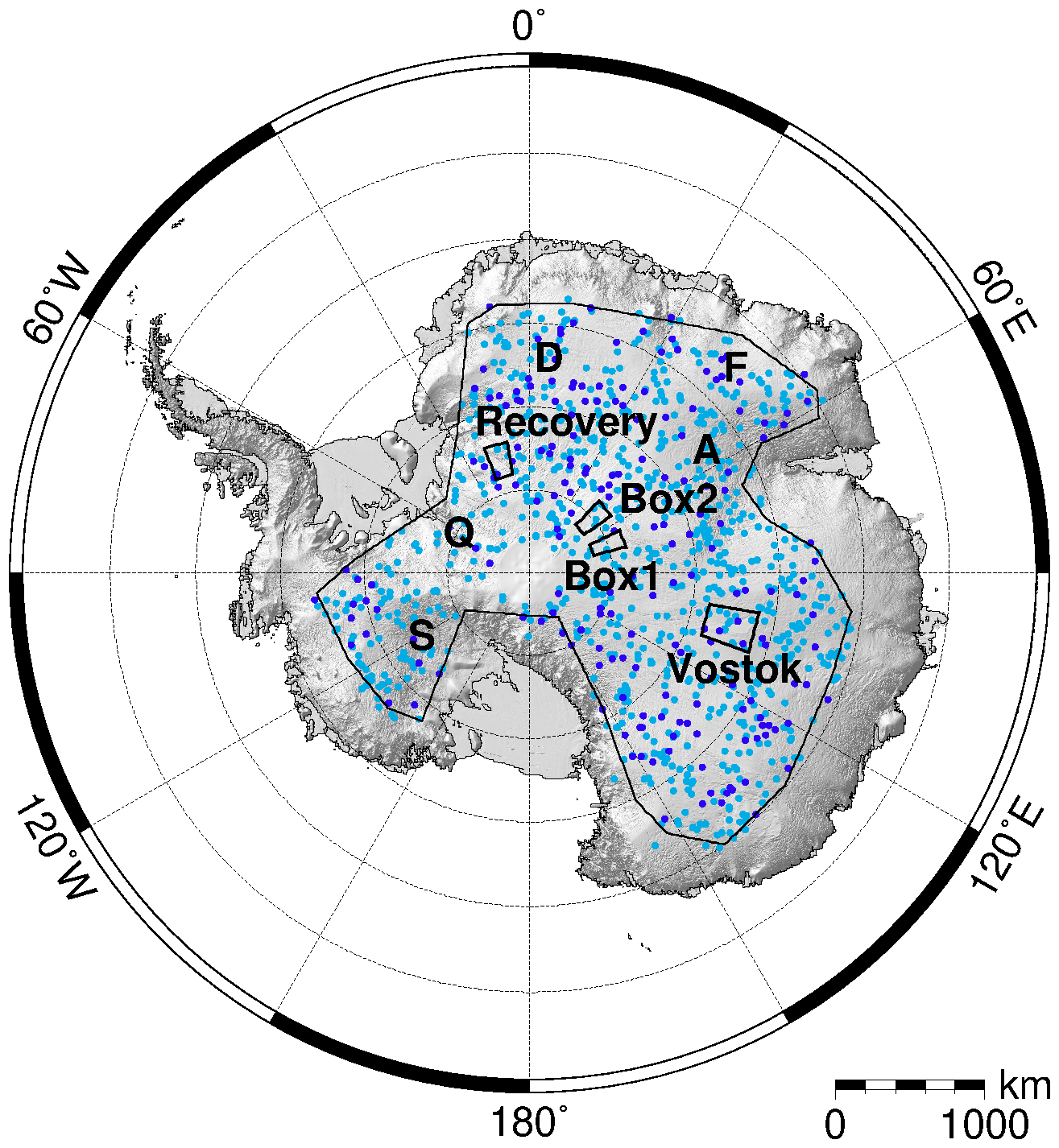
Figure 1Overview of the four selected regions used in the analysis. The dots indicate the randomly selected locations at which the waveforms are simulated. The light-blue dots represent the locations used for training (80 %), while the dark-blue dots represent the locations used for testing the ConvNet (20 %).
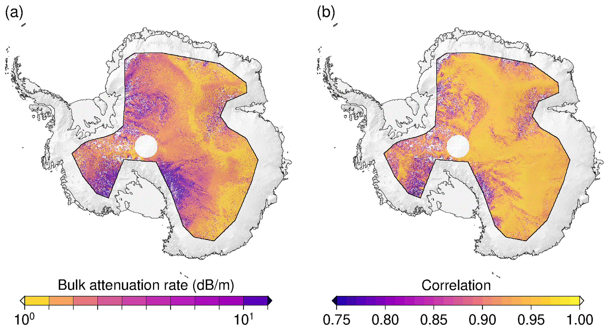
Figure 2Results of the test in which a flat-surface waveform model was fitted to real CryoSat-2 waveforms by adjusting the attenuation LA as the only parameter. (a) Gridded median of the attenuation rate estimated by an MLE fit. (b) Median of the correlation between the observed and fitted waveforms.
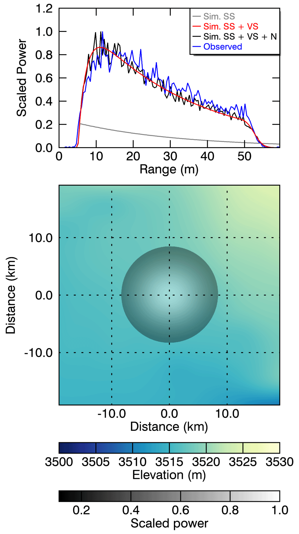
Figure 3An example of the different simulation steps for a typical waveform over Lake Vostok. The blue line denotes the observed CryoSat-2 LRM waveform, and the grey line represents the simulated surface (SS) waveform based on Eq. (1). The red line represents the simulated waveform with volume scattering (SS + VS), based on Eq. (3), while the black line depicts the final simulated waveform, which includes surface and volume scattering as well as noise (SS + VS + N), as given in Eq. (5). The lower panel represents the 2D elevation model as well as scaled , which is mainly controlled by the Gaussian antenna pattern.
2.2 AWI-ICENet1
We use a ConvNet frequency f to model the relationship between a (real or simulated) waveform Ψ and the corresponding retracked range r – i.e. the network provides an estimate () of the retracked range, which corresponds to the true surface, based on the provided input data. During training, only simulated waveforms are used. The network is then applied to real waveforms during inference.
The ConvNet used is similar to the 1D ConvNet used by Fayad et al. (2021). It consists of six blocks of stacked convolutional layers along with rectified-linear-unit (ReLU) activation functions, batch normalization, maximum pooling, and drop-out layers (with overlapping pooling windows similar to those used by Krizhevsky et al., 2012). This differs from the approach of Fayad et al. (2021), who used strided convolutional layers instead of pooling layers to reduce the number of parameters that need to be learnt. In our network design, batch normalization is applied after activation, whereas in the network used by Fayad et al. (2021), this occurs the other way around. The final feature layer is flattened and processed by a fully connected layer with 128 units. Since the waveforms consist of 1D input data, all layers and operations are 1D as well. Figure 4 shows an overview of the network architecture.
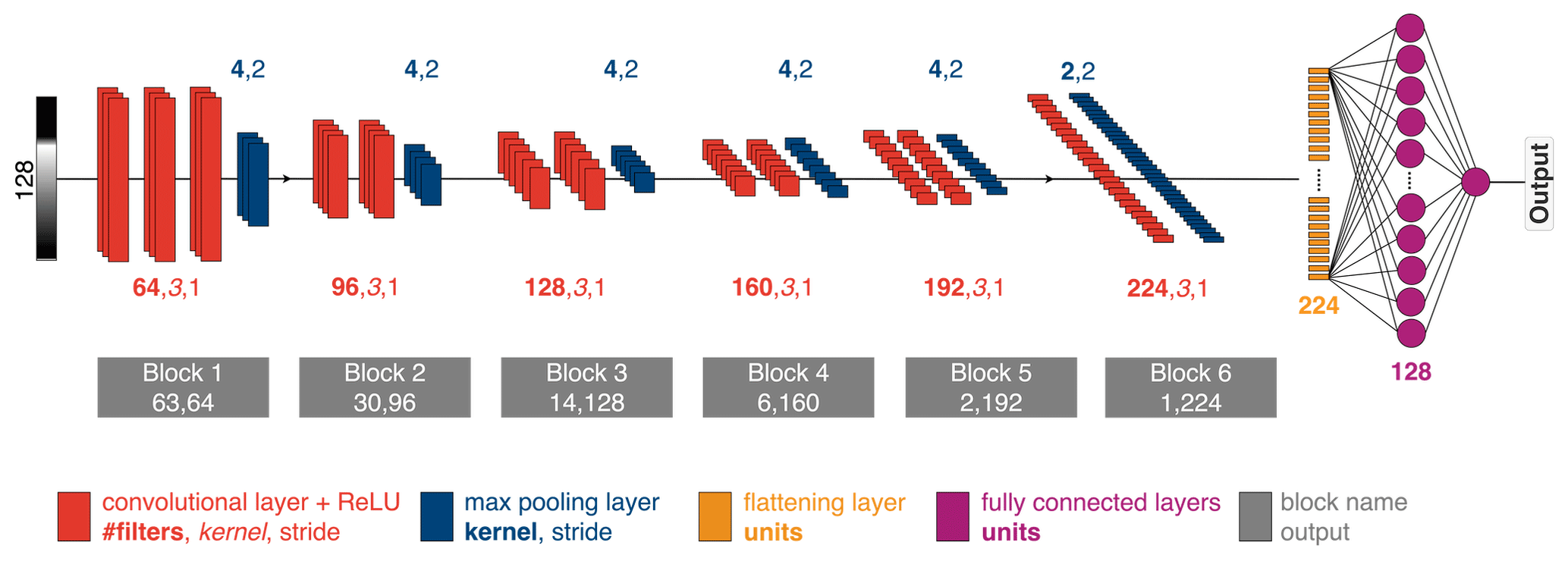
Figure 4A ConvNet is used to map an individual waveform to its corresponding range that correlates with the actual surface. We use standard combinations of convolutions, ReLU, batch normalization, maximum pooling, and drop-out layers. The final feature layer is flattened and used as input to a fully connected layer.
The cost function ℒ is a standard mean-squared-error (MSE) loss between the true and estimated ranges of the simulated waveform. The MSE is calculated as follows:
where ℬ⊂𝒟Tr is the batch, i.e. a subset of the training set 𝒟Tr.
The network is implemented in TensorFlow and trained for 25 epochs with a batch size of 128 using an Adam optimizer (Kingma and Ba, 2014) with level-2 (L2) regularization.
We split the available training data into five different folds and perform five independent runs, using four folds as training data 𝒟Tr and the fifth fold as test data 𝒟Te. Performance is averaged over these five runs. Model performance is assessed via the MSE,
the mean absolute error (MAE),
and the root-mean-squared error (RMSE),
2.3 Satellite altimetry data
In this study, we use CryoSat-2 Level 1B products (including measured waveforms) and Level 2I products (including range estimates by the ESA retracker) from the Baseline-E Low Resolution Mode (LRM) provided by the European Space Agency (ESA). We make use of the ICE1 and ICE2 retracker solutions given in the Level 2I product and, following Helm et al. (2014), apply the TFMRA and the newly developed AWI-ICENet1 retracker to the Level 1B waveform product. ICE1 is based on a threshold-centre-of-gravity (TCOG) retracker (Wingham et al., 1986; Davis, 1997), while ICE2, the University College London (UCL) land ice retracker, fits a Brown model (Brown, 1977) adapted for CryoSat-2. To analyse the performance of AWI-ICENet1 in comparison to the other three retrackers, we use the “ATL06.006” ICESat-2 data product provided by NASA (Smith et al., 2023). We use data from all six beams within the time range from January 2019 to December 2021. Instead of using the quality flag given in the ATL06.006 product, we filter the data based on version 2 of the REMA (an Antarctic elevation model), using a 1 km pixel resolution (Howat et al., 2022), and version 4.1 of the ArcticDEM mosaic (a high-resolution, high-quality digital surface model of the Arctic), using a 500 m pixel resolution (Porter et al., 2023). All data points with a difference larger than ± 100 m are excluded from further processing.
2.4 Elevation change and empirical corrections for the effects of time-variable radar penetration
Surface elevation change (SEC) processing, as applied by various groups, uses different strategies to minimize the effect of radar penetration. In most cases, the backscatter and/or additional waveform shape parameters (such as the leading-edge width (LEW) and trailing-edge slope (TES)), estimated by the ICE2 retracker introduced by Legresy et al. (2005) and Frappart et al. (2016), are used. These waveform parameters are not provided by other retrackers, such as the offset-centre-of-gravity (OCOG) retracker from Wingham et al. (1986), the threshold-centre-of-gravity (TCOG) retracker from Davis (1997), or the threshold first-maximum retracker algorithm (TFMRA) from Helm et al. (2014). Here, we make use of the LEW and backscatter from the Level 2I ICE2 and ICE1, respectively, provided by the ESA LRM. The decision to use the backscatter from ICE1 for all retrackers is based on the lower sensitivity of the OCOG amplitude to speckle noise, which results in the backscatter of successive waveforms being less noisy while preserving large-scale and time-dependent fluctuations. After retracking, the georeferenced surface elevation is determined for each of the retracking approaches using orbital information, such as information on altitude, latitude, and longitude, along with additional geophysical corrections included in the ESA products. In addition, the refined slope correction (Roemer et al., 2007) is applied to relocate the echo to its point of closest approach. This results in a large point cloud of georeferenced elevation measurements for each of the retrackers. Li et al. (2022) developed the leading-edge point-based (LEPTA) method, an improved version of the relocation slope correction which includes points in the underlying DEM that contribute to the rise in the leading edge. Their results show an improved cross-point error (CPE) between CryoSat-2 and ICESat-2 compared to the method of Roemer et al. (2007). However, as we only consider intra-mission cross-point errors and apply the same slope correction to all retracker solutions, the slope correction method does not play a role in our CPE analysis.
The interpolated elevation anomaly product and rates of elevation change () are generated using a slightly different approach, as described in McMillan et al. (2016), Schröder et al. (2019), and Nilsson et al. (2022). For each pixel with a size of 1 km × 1 km, we collect all georeferenced data points within a variable distance ranging from 500 to 2500 m (step width: 500 m) and correct for topography using a bilinear interpolation of the REMA DEM and/or ArcticDEM, rather than fitting a linear or quadratic surface – an approach used by McMillan et al. (2016), Schröder et al. (2019), and Nilsson et al. (2022). The variable search radius is enlarged stepwise until a threshold number of points is reached. This threshold is defined to cover at least 75 % of the selected time period (nmonths) and meet the following criteria – for CryoSat-2, it corresponds to nmonths⋅6, and for ICESat-2, due to the higher data coverage resulting from six beams and less along-track point spacing, it corresponds to nmonths⋅48. This kind of processing allows us to minimize uncertainties due to unresolved topography within the search radius while maintaining enough data points for linear regression by keeping the search radius as low as possible. Processing costs for pixels with very dense data coverage in the interior of Antarctica are kept low by selecting a small radius (and thus fewer data points). At the same time, fewer unobserved pixels remain in areas of coarse data coverage as the search radius can be enlarged up to 2500 m. We then estimate rates of elevation change using linear regression for each pixel with sufficient data coverage (with the criteria being that of selected time period and npoints>nmonths), without using additional information, e.g. LEW, the TES, backscatter, or seasonal components. The residuals are averaged to monthly residuals per pixel. Both gridded products – the trend and the monthly residual grids – are finally interpolated using inverse distance weighting with a variable radius to form the final interpolated grids with a 5 km posting. Furthermore, the backscatter and LEW information are processed in the same way, i.e. without any trend or topographic correction. We calculate different variants of corrections for transient-penetration effects using empirical linear relations between Δ h and LEW; Δ h and backscatter; or Δ h, LEW, and backscatter. Instead of performing this in the context of multi-parameter fitting, as in Flament and Rémy (2012), Simonsen and Sørensen (2017), and Schröder et al. (2019), we apply it to spatially interpolated monthly anomalies in Δ h, LEW, and backscatter, following the approach of Nilsson et al. (2022). We assume that changes in the electromagnetic properties of the ice sheet surface are driven by atmospheric processes that affect temperature and surface density at the kilometre scale, which may explain the time-varying elevation anomalies (hereafter referred to as Δ h), as shown by Lacroix et al., 2008. Our approach of applying the correction to averaged, interpolated products reduces the high uncertainty in single waveform parameter estimates. This is reflected in the high correlations between Δ h and anomalies in LEW and backscatter, as presented in Figs. A5, A6, A7, and A8 for Greenland and Antarctica. Our final product contains four monthly elevation estimates for each of the four retracker solutions used to investigate Δ h and derive . These are compared with those derived by ICESat-2 using the same processing strategy. The estimates are as follows:
-
Δ h and without any correction
-
LEW-corrected Δ h and
-
Backscatter-corrected Δ h and
-
LEW- and backscatter-corrected Δ h and .
To evaluate the performance of the new AWI-ICENet1 retracker, different tests are conducted, which are summarized and structured as follows. First, AWI-ICENet1 is evaluated using statistical metrics based on the simulated test data set, such as the MSE. Learning curve and K-fold cross-validation statistics are shown. Second, the simulated data set is retracked using the TFMRA from Helm et al. (2014) and compared to data from AWI-ICENet1. Third, the new retracker is applied to CryoSat-2 LRM data, and a monthly cross-point-error analysis is carried out in four selected regions of interest (ROIs) in Antarctica to assess the retracker's ability to provide reliable elevation estimates in areas with varying surface topography and bulk attenuation rates. Fourth, the monthly cross-point-error analysis is carried out across the LRM zone using all four retrackers (AWI-ICENet1, the TFMRA, and the ESA products ICE1 and ICE2). To assess the retracker's performance in terms of its ability to minimize transient-penetration effects, the monthly elevation anomaly product is evaluated within the ROIs and spatially across the whole LRM zone of Antarctica and Greenland. Finally, empirical corrections are applied to reduce time-variable penetration bias for all retrackers and are evaluated.
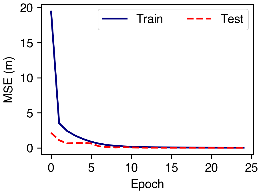
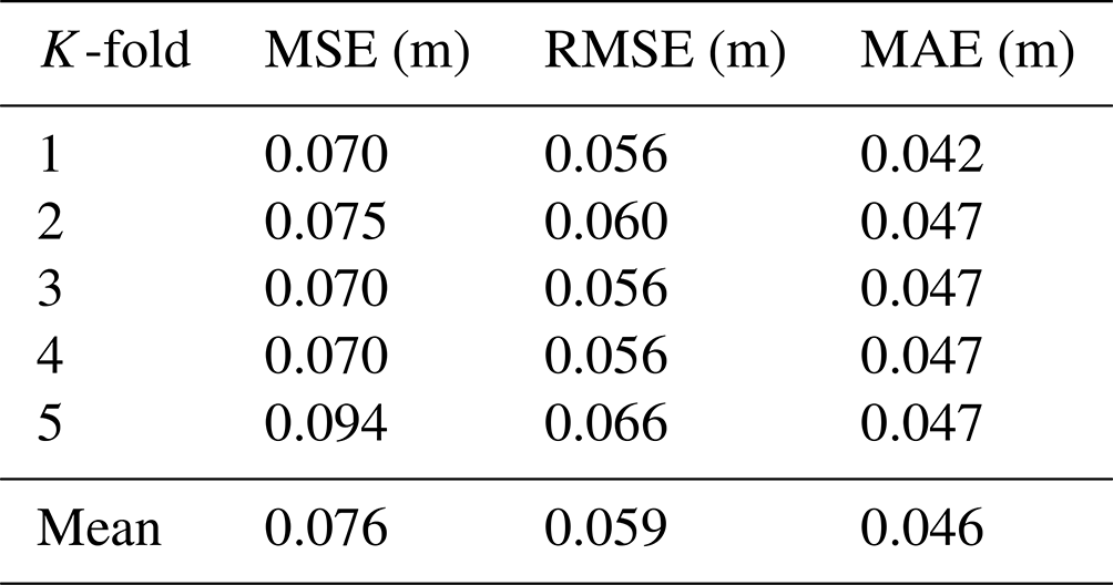
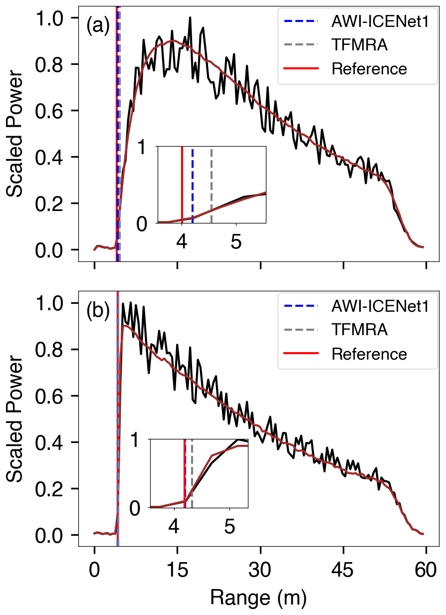
Figure 6Examples of simulated waveforms for (a) low LA and (b) high LA. The initial noise-free waveform is indicated by the red line, and added noise is indicated by the black line. The reference range is displayed as a vertical bar in red, and the TFMRA- and AWI-ICENet1-retracked ranges are superimposed in grey and blue, respectively. The insets show a zoomed-in view of the leading edge, where the retracking takes place.
3.1 AWI-ICENet1 results for simulated waveforms
We evaluated the ConvNet performance using the MAE, MSE, and RMSE – as given in Eqs. (7), (8), and (9) – and by examining the learning curve of the MSE for both the training and test data sets. The learning curve of our final model is shown in Fig. 5. Here, the MSE of the training and test data gradually decreases and reaches a constant plateau after approximately 10 epochs. To assess whether the model architecture provides similar metrics for different training and test data, we applied a 5-fold cross-validation method, meaning that the same input data set is split into five different parts using an split factor for training and testing. The results of the different folds are listed in Table 1. They show nearly identical values, indicating consistent, repeatable learning independent of the training data set. Our final model, which was a hold-out model with an RMSE of 0.056 m and an MAE of 0.042 m, was considered for application to real data and further analysis.
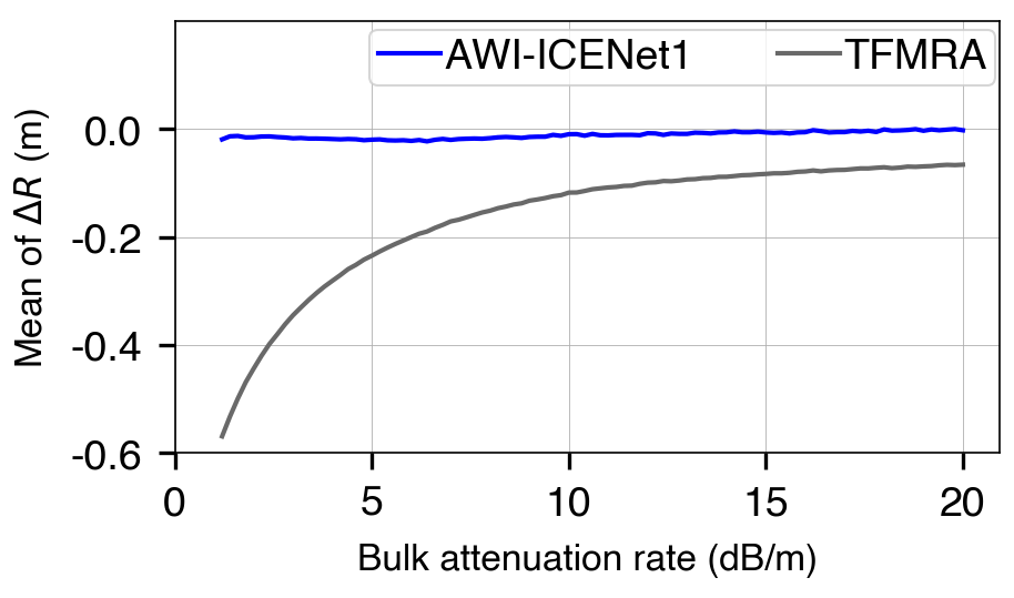
Figure 7Comparison of the mean ΔR with respect to the bulk attenuation rate between AWI-ICENet1 and the TFMRA.
To evaluate the performance of the retracker, we estimated the difference () between the retracked range (RRT) and the reference range (Rref). In addition, we applied the TFMRA to the same set of simulated waveforms and estimated ΔR as well. In Fig. 7, the mean values of ΔR for AWI-ICENet1 and the TFMRA are presented. The statistics were calculated for all locations across Antarctica, subdivided into bins of bulk attenuation rates. Here, the influence of high volume scatter due to low LA on range retrieval is clearly shown. For low LA, we observed only a small offset (<0.03 m) in the AWI-ICENet1-retracked surface elevation compared to the true surface. In contrast, ΔR pertaining to the TFMRA forms a kind of exponential function, with differences of up to −0.5 m for low LA, as presented in Fig. 7.
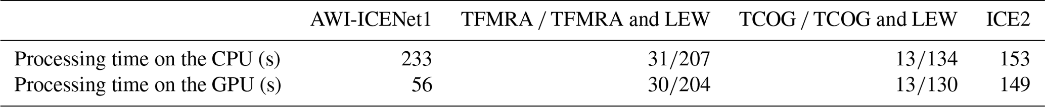
As a performance test, we ran the retracking on one of the CPU and GPU compute nodes of the high-performance cluster at the Alfred Wegener Institute, Helmholtz Centre for Polar and Marine Research. In addition to the TFMRA, we applied the TCOG retracker and an adapted version of the functional fit of the ICE2 retracker, as described in Legresy et al. (2005). To estimate the leading-edge width (LEW) based on the TFMRA and the TCOG retracker, we ran the retracking for different threshold levels (THLs), ranging from 5 % to 80 %. For each THL, a retracked position (RT) is determined. The LEW is the inverse of the linear regression coefficient and is estimated for each waveform as follows: , where THL corresponds to . Results of the performance test are shown in Table 2.
Table 2Results of the performance test for different retrackers. Retracking was applied to 1 million waveforms.
3.2 AWI-ICENet1 results for observed waveforms
In this section, the final AWI-ICENet1 retracker is applied to the entire CryoSat-2 time series. For each of the ESA Level 1B 20 Hz waveforms, a range is retracked and combined with precise orbit information (e.g. information on latitude, longitude, and altitude) to form a point cloud of georeferenced surface elevations. The cross-point-error analysis is carried out on precise orbits. To derive elevation and elevation change products for further applications, a slope-corrected point cloud data set is generated using relocation slope correction, as described by Roemer et al. (2007).
3.2.1 Cross-point-error analysis
To avoid time-dependent differences due to changes in radar volume scattering, our accuracy measure for the individual solutions is based on monthly cross-point-error (CPE) analysis across the entire Antarctic ice sheet. A CPE is defined as the elevation difference between ascending and descending tracks at cross points (CPs). In total, more than 3 million CPs from 130 months are used. We filter outliers using the following criterion: m. Finally, a grid with a 5 km × 5 km pixel resolution, based on the mean and standard deviation (SD), is calculated from all CPEs. Figures 8 and 9 show the time evolution of the median and SD of the CPEs for four selected regions, which are shown in Fig. 1. In the Box1 area (Fig. 8a), we find a significant negative CPE for the TFMRA and both ESA retrackers, with the largest CPE corresponding to the ESA ICE2 retracker. AWI-ICENet1 has a very low CPE and performs best in this area. In Box2, the picture is similar, but the CPE lies within the positive range, with the ESA ICE2 retracker once again showing the highest CPE (Fig. 8b). The SD, displayed in panels (a) and (b) of Fig. 9, also shows exceptionally high values for the ESA ICE2 retracker. The other retrackers have similar SDs, around 20 cm, in Box1 and Box2. Next, we consider two regions with specific topographic settings (both areas are shown in Fig. 1): the Vostok region, characterized by a very flat terrain with minimal surface undulations, and the “Recovery” region, which is more complex and has steeper surface slopes of up to 1° and medium-scale topographic undulations. The results for the median CPE are presented in Fig. 8c and d. For both areas, the median CPE is lower than for the two box areas, with the range peaking at 20–30 cm. Again, the ESA ICE2 retracker shows the highest CPE across the entire time period for the Vostok and Recovery areas. The new AWI-ICENet1, the TFMRA, and the ESA ICE1 retracker have median and SD CPE values of a similar order of magnitude, with only slight differences. Temporal variability is higher in the Recovery area than in the Vostok region.
The strong differences in surface characteristics also become evident when using the SD of the CPEs for comparison. In the Recovery area, the SD of the CPEs ranges from about 0.5–1.5 m, roughly 3 times higher than that in the Vostok area and the two box areas. In all cases, the trends in the median and SD of the CPEs have been rather stable over the years, with a few exceptions. In the Box2 area, we find a decrease in the median CPE for the ESA ICE2 retracker from 2018 onwards. Additionally, some incremental changes (a few centimetres in size) are observed by the ESA ICE1 retracker and TFMRA, while AWI-ICENet1 remains constant over time. The time series of the SD of the CPEs also show generally stable trends, with a few exceptions: in Box1 and Vostok, we find a peak in all retrackers except the ESA ICE2 retracker, whereas the trend in the median for Box2 is not reflected in the SD. The high temporal variability in the SDs of the CPEs in the Recovery area prevents us from analysing trends, but all retrackers show variability of a similar magnitude.
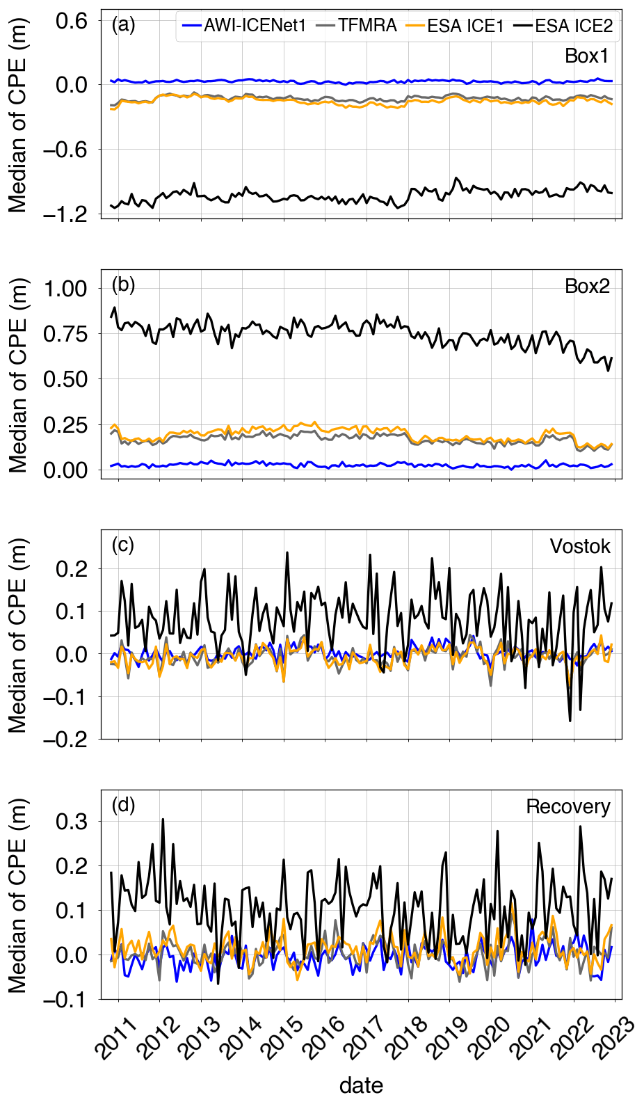
Figure 8Time series of the median cross-point errors for different areas. Cross-point errors are determined at a monthly resolution for each region.
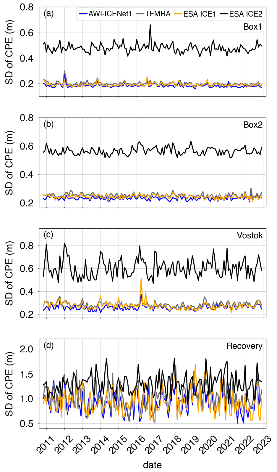
Figure 9Time series of the standard deviation of cross-point errors for different areas. Cross-point errors are determined at a monthly resolution for each region.
In the next step, we broaden the view and discuss the CPEs over the entire ice sheet. Figure 10 displays the time series of the SD of the CPEs for the complete LRM zone of Antarctica, covering the 12-year observational time period of the CryoSat-2 era. Here, AWI-ICENet1 and the ESA ICE1 retracker are similar in terms of the SD of the CPEs, whereas the TFMRA exhibits considerably higher SD across the entire ice sheet. The ESA ICE2 retracker has a particularly high SD – almost twice as large as that of the other two. The temporal variability is rather low and shows no trends for any of the four retracker solutions. The pan-Antarctic gridded median and SD of the CPEs are shown in Figs. 11 and 12. The results reveal that the crossover difference is reduced by roughly a factor of 4 to 5 for ICE1 and the TFMRA compared to ICE2 (note the different value range in panel (c) of Fig. 11). However, there are remaining CPEs with alternating signs, up to ±0.3 m, across Antarctica, including a prominent pattern in the interior of East Antarctica, which is close to the polar gap. This pattern, discussed below, is entirely eliminated with AWI-ICENet1, as displayed in panel (a) of Fig. 11. AWI-ICENet1 also exhibits a low median CPE with AWI-ICENet1 can be also seen close to the ice divides north of Dome Fuji (indicated by F in Fig. 1), in southern Dronning Maud Land (D), in the topographically complex areas of the Siple Coast (S), and in the drainage area of the Amery Ice Shelf (A). The SDs of the CPEs shown in Fig. 12a, b, and d are very similar for AWI-ICENet1, the ESA ICE1 retracker, and the TFMRA, respectively, and are a factor of 4 to 5 smaller than those for the ESA ICE2 retracker (Fig. 12c). In general, the lowest values are found in the flat interior, and the highest values are found in the sloped areas with complex topography. This is consistent with our findings for the four test areas, where the highest SD of the CPEs is observed in the Recovery area with the roughest topography.
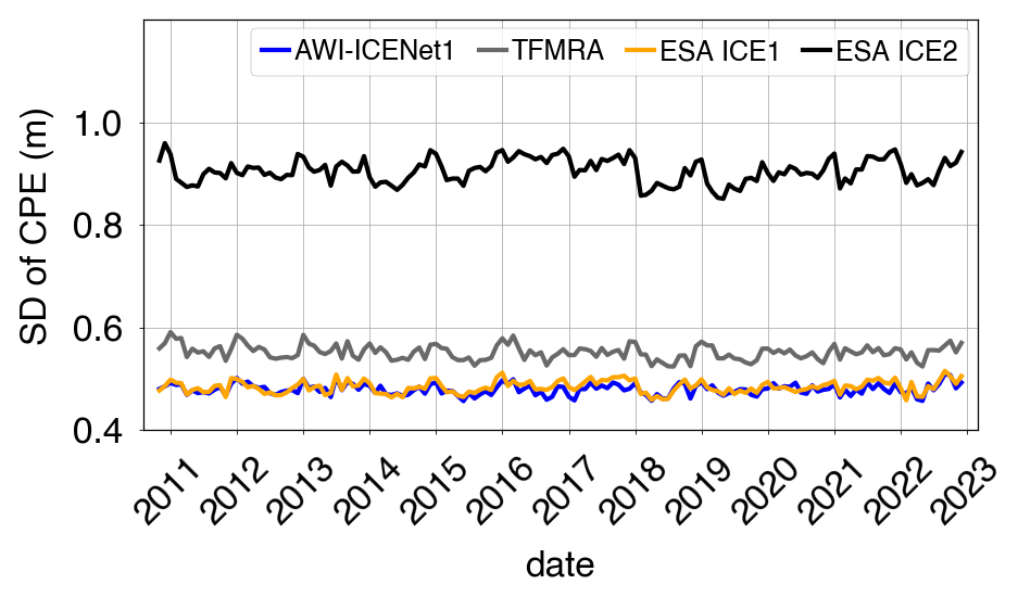
Figure 10Time series of the standard deviation of cross-point errors across the LRM zone in Antarctica. Cross-point errors are determined at a monthly resolution.
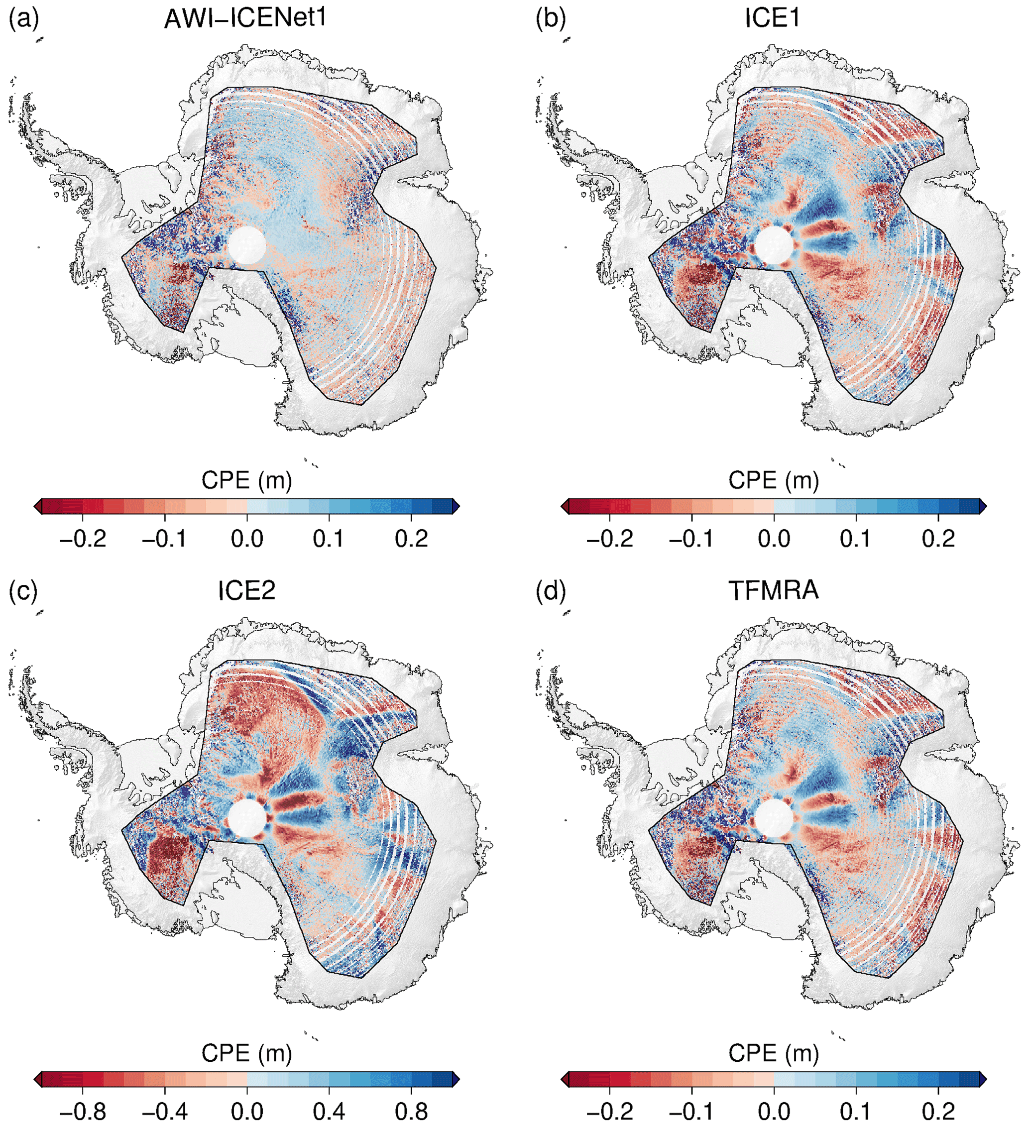
Figure 11Spatial distribution of the median of the cross-point errors across the LRM zone in Antarctica for all four retrackers. Cross-point errors are determined at a monthly resolution for the time period from January 2011 to December 2022. The median is determined for each 5 km × 5 km pixel. Please note that panel (c) has a different range for the colour bar compared to the other three panels.
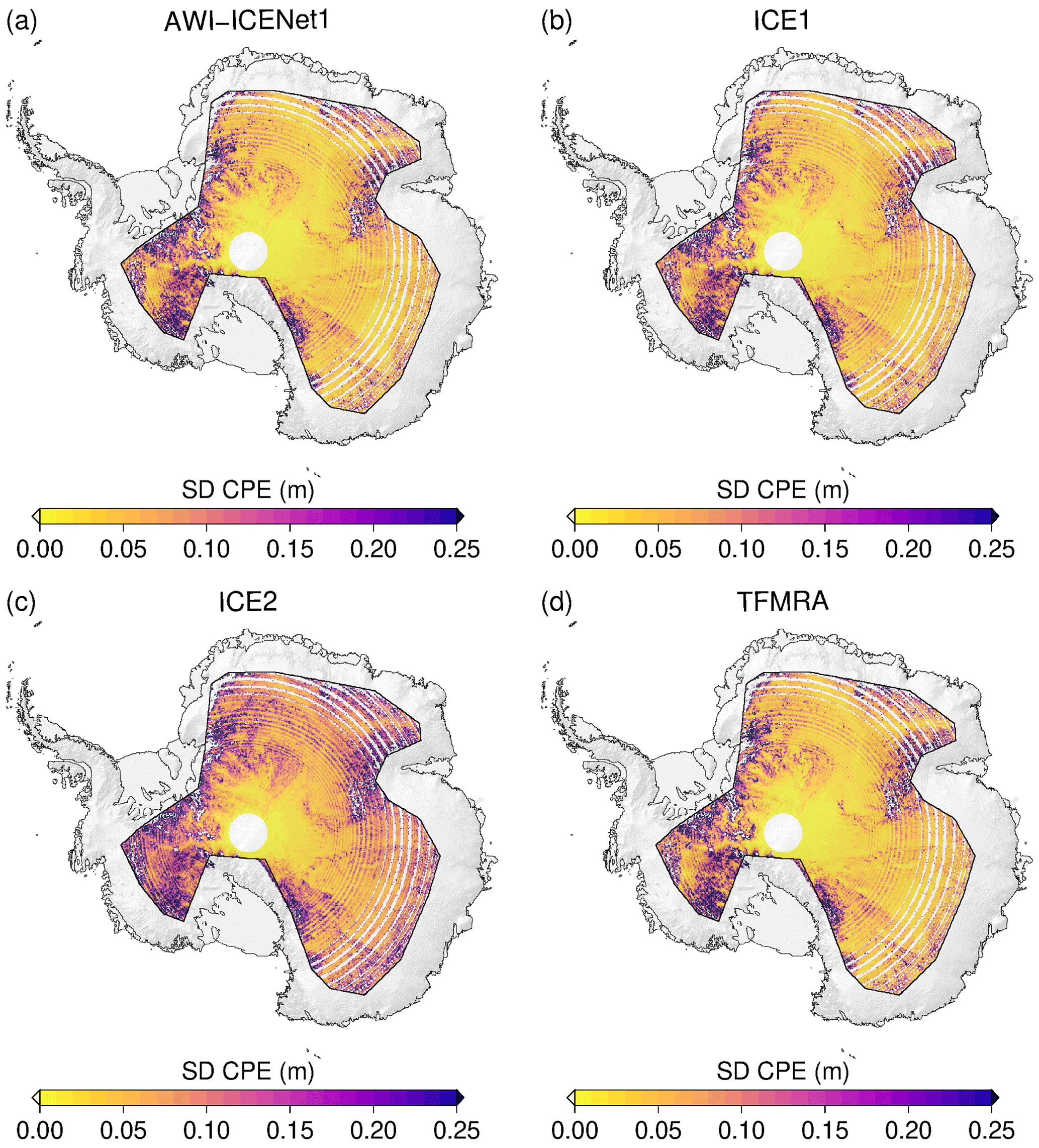
Figure 12Spatial distribution of the standard deviation of cross-point errors across the LRM zone in Antarctica for all four retrackers. Cross-point errors are determined at a monthly resolution for the time period from January 2011 to December 2022. The standard deviation is determined for each 5 km × 5 km pixel.
3.2.2 Transient penetration
In this section, we analyse the time-dependent variability in Δ h, which has been widely discussed in the literature as corresponding to transient penetration or penetration bias due to changes in firn properties (e.g. Davis and Zwally (1993), Michel et al. (2014), and Slater et al. (2019)) for various retrackers. To this end, in Fig. 13, we present Δ h and its standard deviation, SD(Δ h), for all retrackers and across the entire CryoSat-2 time period for the Lake Vostok region, a region that has exhibited a stable surface height over the last decade (Richter et al., 2014). Except for AWI-ICENet1, all retrackers show strong variability, with the ESA ICE2 retracker exhibiting the largest range (up to 0.8 m). The temporal variability in the ESA ICE1 and ICE2 retrackers and the TFMRA are correlated, although the ESA ICE1 retracker and TFMRA exhibit lower magnitudes compared to the ESA ICE2 retracker. The new AWI-ICENet1 exhibits Δ h amounting to only a few centimetres, with minor temporal variability and a slight increase from 2021 onwards. The SD of the elevation anomalies (Fig. 13b) is largest for the ESA ICE2 retracker, while the ESA ICE1 retracker and TFMRA exhibit similar SD values, significantly lower than those exhibited by the ESA ICE2 retracker, although the temporal evolution has the same form as that pertaining to the ESA ICE2 retracker. AWI-ICENet1 exhibits not only low Δ h but also low SD(Δ h). Figure 14 presents the Δ h and SD(Δ h) values for a 5000 km2 high-elevation area on the North Greenland plateau (79° N, 45° W). Large sudden increases of more than 1.0 m for the ESA ICE2 retracker are observed in July 2012 and August 2018. Here, the TFMRA and ESA ICE1 retracker also experience an increase of 0.3 m, whereas AWI-ICENet1 stays at the same level. Both events can be related to unusual heat waves transporting warm air to high elevations, resulting in surface melt conditions, as reported by the Danish Meteorological Institute (DMI) portal. In all other months, the anomalies are correlated and follow a similar trend but with strong differences in the observed magnitudes, with AWI-ICENet1 showing the smallest values and the ESA ICE2 retracker showing the highest values. For the SD of the elevation anomalies (Fig. 14b), we observe the same pattern as that for the Vostok area, with the lowest values corresponding to AWI-ICENet1 and the highest values corresponding to the ESA ICE2 retracker. In the following, we will discuss how this relates to the findings of other studies and continue inspecting the spatial distribution of Δ h.
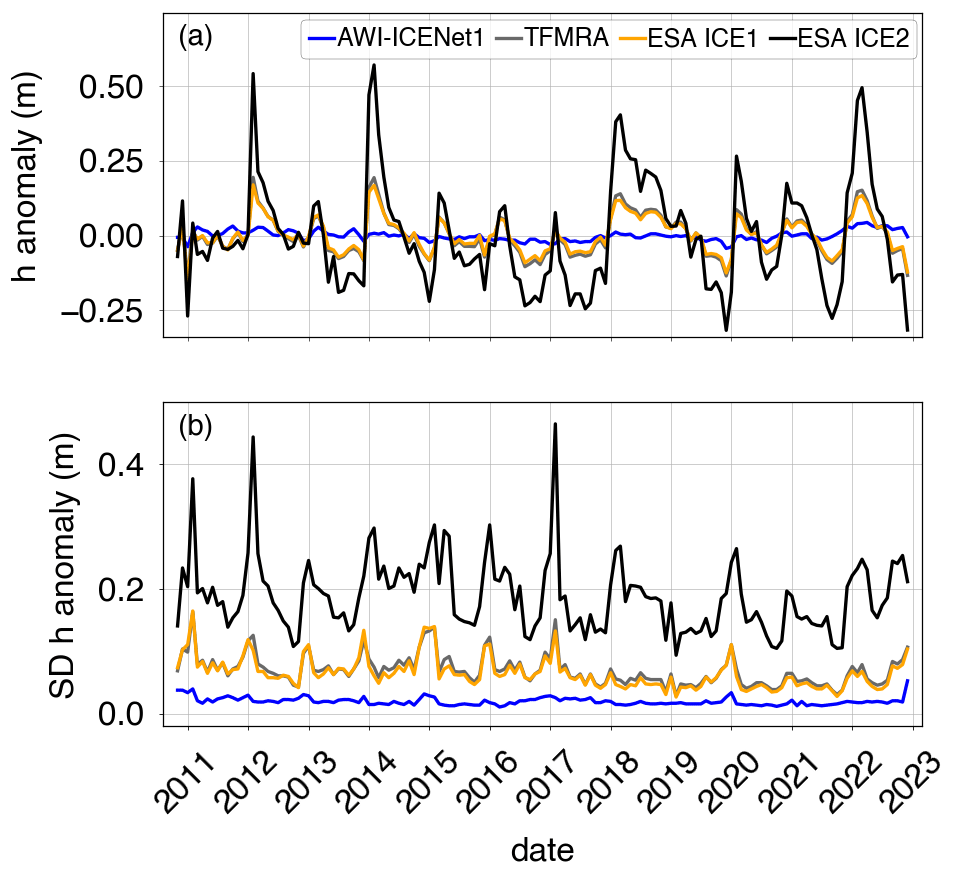
Figure 13Time-dependent mean value (a) and standard deviation (b) of the elevation anomalies pertaining to the Vostok region. The elevation anomalies are based on grid with a 5 km × 5 km pixel resolution, derived from the spatially interpolated monthly residuals of the elevation trend estimation.
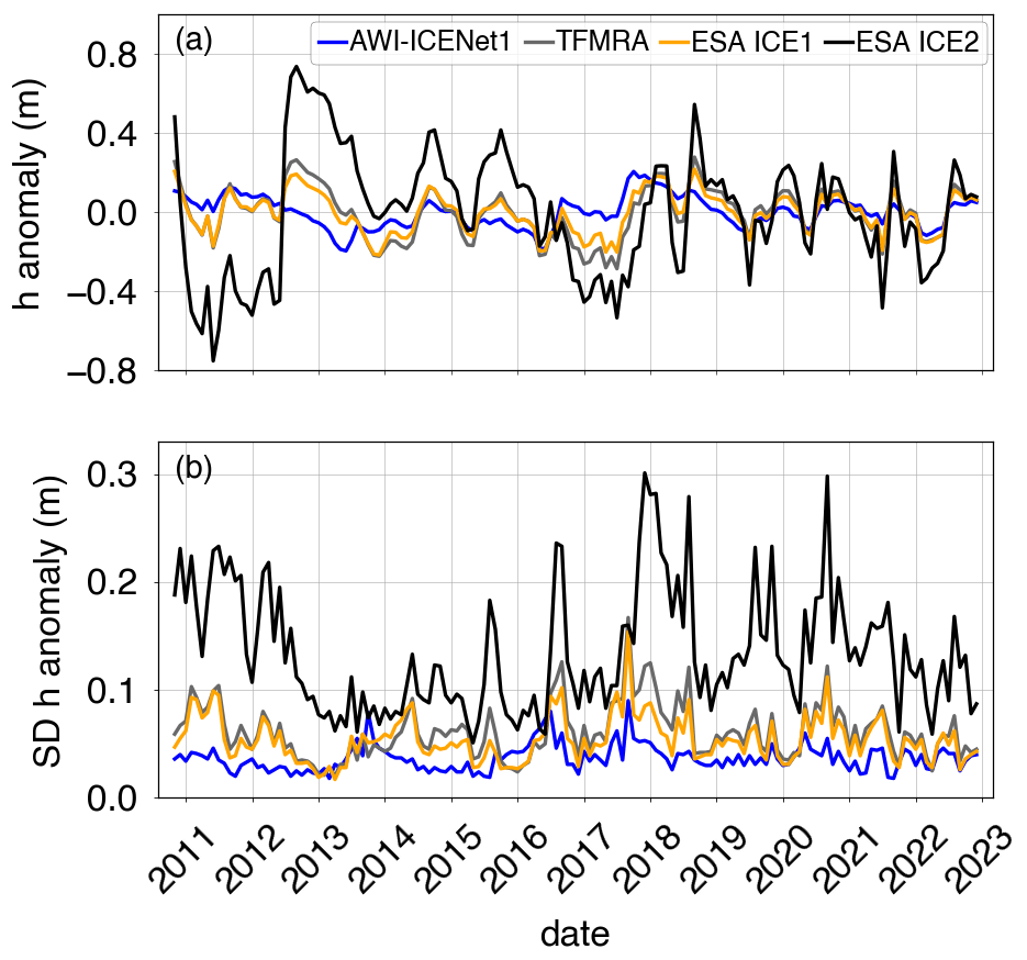
Figure 14Time-dependent mean value (a) and standard deviation (b) of the elevation anomalies pertaining to the North Greenland region. The elevation anomalies are based on grids with a 5 km × 5 km pixel resolution, derived from the spatially interpolated monthly residuals of the elevation trend estimation.
Figure 15 presents the spatial distribution of SD(Δ h). Here, the standard deviation is calculated for each pixel (5 km posting). The ESA ICE1 retracker and TFMRA have a close spatial distribution and magnitude, with the largest elevation anomaly observed along the Siple Coast (S in Fig. 1) and the drainage basins in Queen Elizabeth Land feeding the Ronne Ice Shelf (Q in Fig. 1). For the ESA ICE2 retracker, the SD of elevation anomalies exceeds 30 cm in an extensive area. The lowest SD of the elevation anomalies is found for AWI-ICENet1, where the largest values are also found in West Antarctica. However, SD(Δ h) for nearly all of East Antarctica is below 5 cm, whereas for the ESA ICE1 retracker and TFMRA, SD(Δ h) ranges from 8–25 cm.
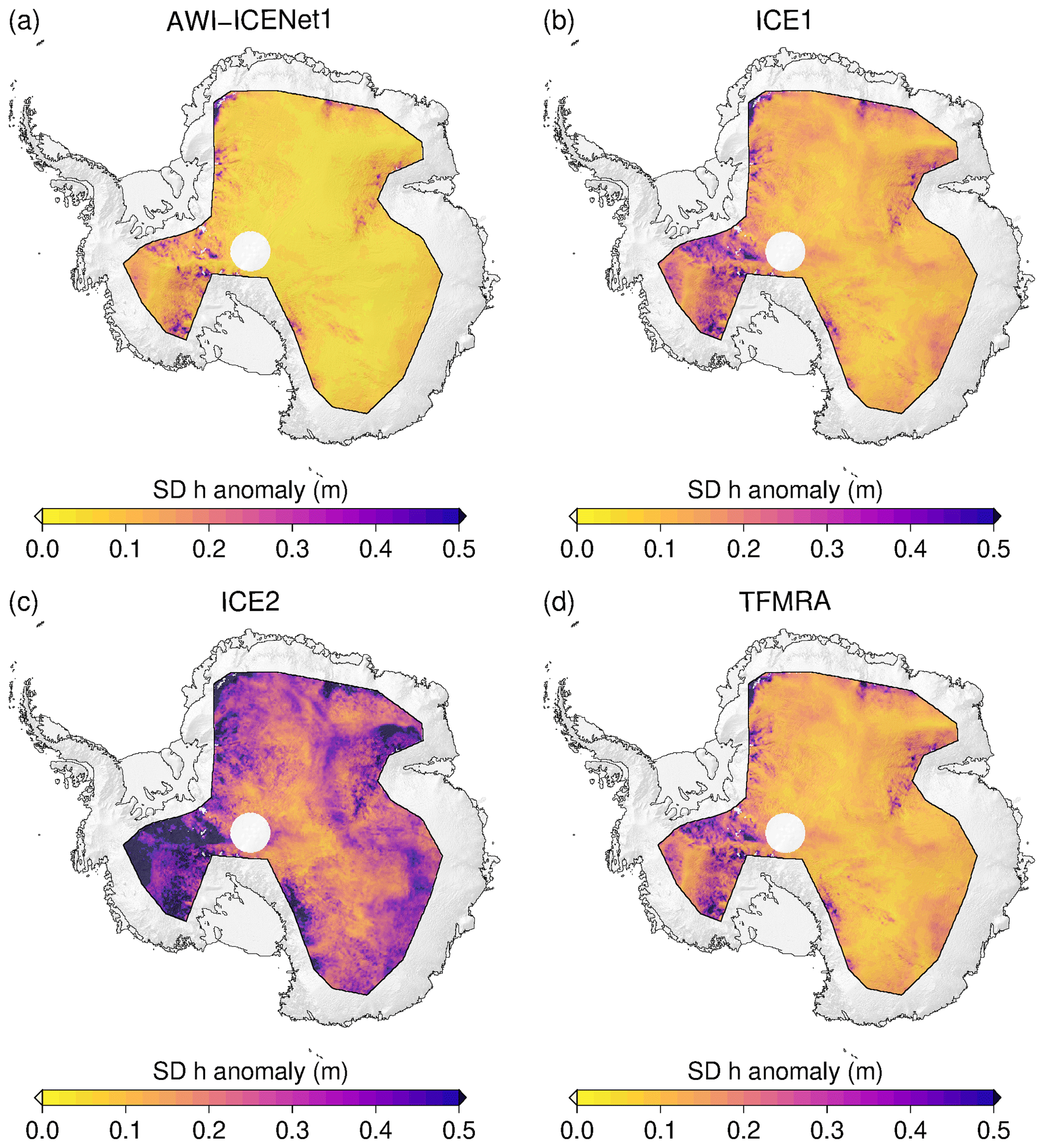
Figure 15Spatial distribution of the standard deviation of the elevation anomalies across the LRM zone in Antarctica for all four retrackers. The elevation anomalies are based on grids with a 5 km × 5 km pixel resolution, derived from the spatially interpolated monthly residuals of the elevation trend estimation. The standard deviation is determined for each pixel across the full time period from January 2011 to December 2022.
3.2.3 Empirical correction of transient penetration compared to AWI-ICENet1
Flament and Rémy (2012), Simonsen and Sørensen (2017), Schröder et al. (2019), and Nilsson et al. (2022) used an empirical relation between the elevation anomalies and backscatter, LEW, and/or the TES to partly reduce the transient-penetration effect. Here, we make use of the same correction, largely following Nilsson et al. (2022). Specifically, we apply the correction to all retrackers, using LEW and backscatter for the Vostok area and LEW only for the North Greenland area, which aligns with the findings of Simonsen and Sørensen (2017). Results for Vostok and North Greenland are shown in Figs. 16 and 17, respectively. In both cases, Δ h is strongly reduced for all retrackers, with exception of AWI-ICENet1. The largest reduction is observed for the ESA ICE2 retracker, but it still shows the largest remaining Δ h, exceeding the values for AWI-ICENet1 by a factor of 2 or higher. The TFMRA and ESA ICE1 retracker are similar and closer to AWI-ICENet1 but still show larger magnitudes. The SD of Δ h is reduced for all retrackers, with the least improvement observed for AWI-ICENet1. However, our new retracker shows the smallest SD, as presented in Fig. 16b. In North Greenland, the sudden positive elevation increase, resulting from a change in the dominant scattering regime caused by the melt events in the summer of 2012 and 2018, is strongly suppressed. The different solutions are now correlated over the years. The smallest remaining Δ h is observed for AWI-ICENet1, followed by the TFMRA and the ESA ICE1 and ICE2 retrackers. For North Greenland, the TFMRA and ESA ICE1 retracker show larger negative and positive deviations from AWI-ICENet1 in the winters of 2013/2014 and 2017/2018, respectively, as shown in Fig. 17a. Moreover, Δ h in North Greenland is more variable than in Vostok, reaching values of 0.1 m for AWI-ICENet1. Around Vostok, only small perturbations of <3 cm are observed with AWI-ICENet1, reflecting the low-accumulation regime in East Antarctica. Figure 18 presents the spatial distribution of the SD of the elevation anomalies corrected with LEW and backscatter. Again, the ESA ICE2 retracker shows the largest anomalies, followed by the ESA ICE1 retracker and the TFMRA. SD(Δ h) is reduced to 4–10 cm for the TFMRA and ESA ICE1 retracker for the majority of the East Antarctic Plateau. For AWI-ICENet1, only a minor reduction in SD(Δ h) could be achieved, with values amounting to less than 4 cm for the majority of East Antarctica. It is worth mentioning that even the corrected TFMRA in Fig. 18d still shows larger values than the uncorrected AWI-ICENet1 in Fig. 15a. To investigate the extent to which the applied correction mitigates the transient penetration for each retracker, we sort the SD(Δ h) values of the uncorrected and corrected Δ h within the LRM zone into bins with a size of 0.02 m, as shown in Fig. 19. The cumulative frequency in Fig. 19a shows that approximately 80 % of the SD(Δ h) values for AWI-ICENet1 are less than 6 cm, whereas this is true for less than 20 % of said values for the TFMRA and ESA ICE1 retracker. The ESA ICE2 retracker exhibits values greater than 15 cm for more than 90 % of the area and values greater than 30 cm for more than 50 % of the area. After correction, as presented in Fig. 19b, 60 % of the area for the TFMRA and ESA ICE1 retracker shows values of less than 6 cm. While the effect of the applied correction is significant for all retrackers except AWI-ICENet1, it is not able to minimize the transient-penetration bias to the same order of magnitude as AWI-ICENet1. Since AWI-ICENet1 experiences only a small reduction in SD(Δ h), we conclude that most of the transient-penetration bias is already corrected by the retracker. Similar results are obtained for the Greenland Ice Sheet but with larger magnitudes of SD(Δ h) in general. Corresponding figures illustrating the spatial distribution of SD(Δ h) and the cumulative distribution are presented in the Appendix in Figs. A11, A12, and A13.
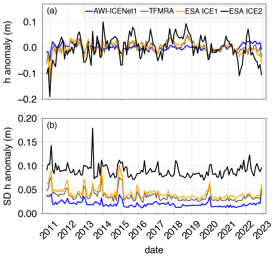
Figure 16Time-dependent mean value (a) and standard deviation (b) of the corrected elevation anomaly pertaining to the Vostok region. The elevation anomalies are based on grids with a 5 km × 5 km pixel resolution, derived from the spatially interpolated monthly residuals of the elevation trend estimation that were corrected for transient penetration using LEW and backscatter.
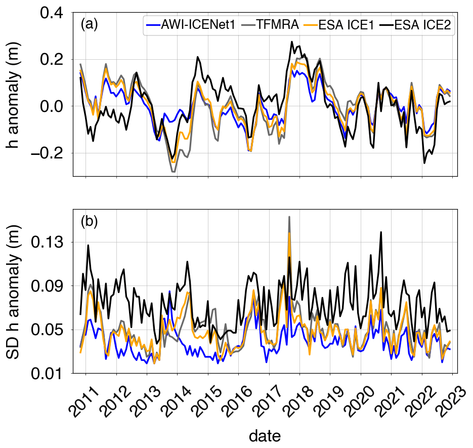
Figure 17Time-dependent mean value (a) and standard deviation (b) of the corrected elevation anomaly pertaining to a region in North Greenland. The elevation anomalies are based on grids with a 5 km × 5 km pixel resolution, derived from the spatially interpolated monthly residuals of the elevation trend estimation that were corrected for transient penetration using LEW only.
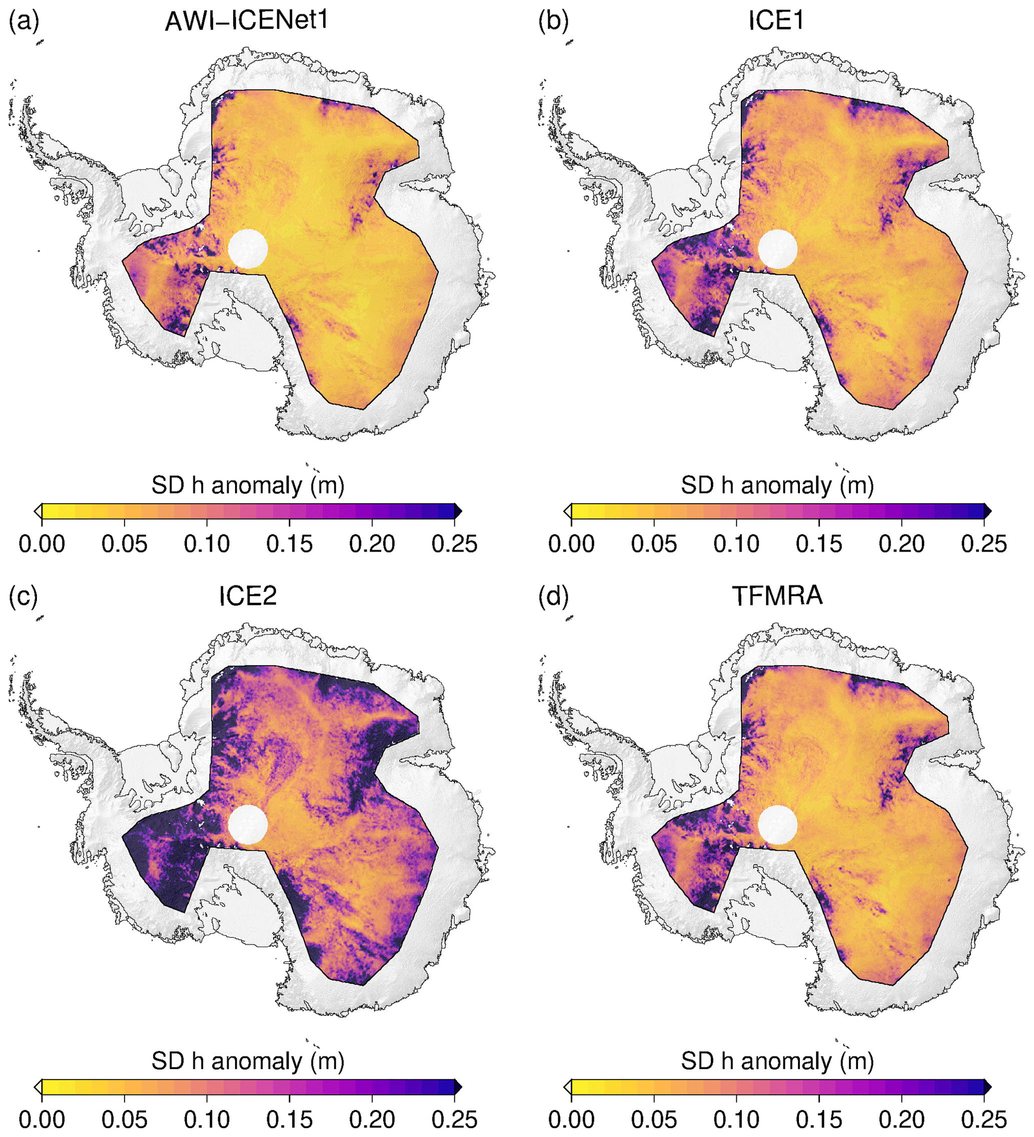
Figure 18Spatial distribution of the standard deviation of the corrected elevation anomaly across the LRM zone in Antarctica for all four retrackers. The elevation anomalies are based on grids with a 5 km × 5 km pixel resolution, derived from the spatially interpolated monthly residuals of the elevation trend estimation that were corrected using correlations with leading-edge width and backscatter. The standard deviation is determined for each pixel across the full time period from January 2011 to December 2022.
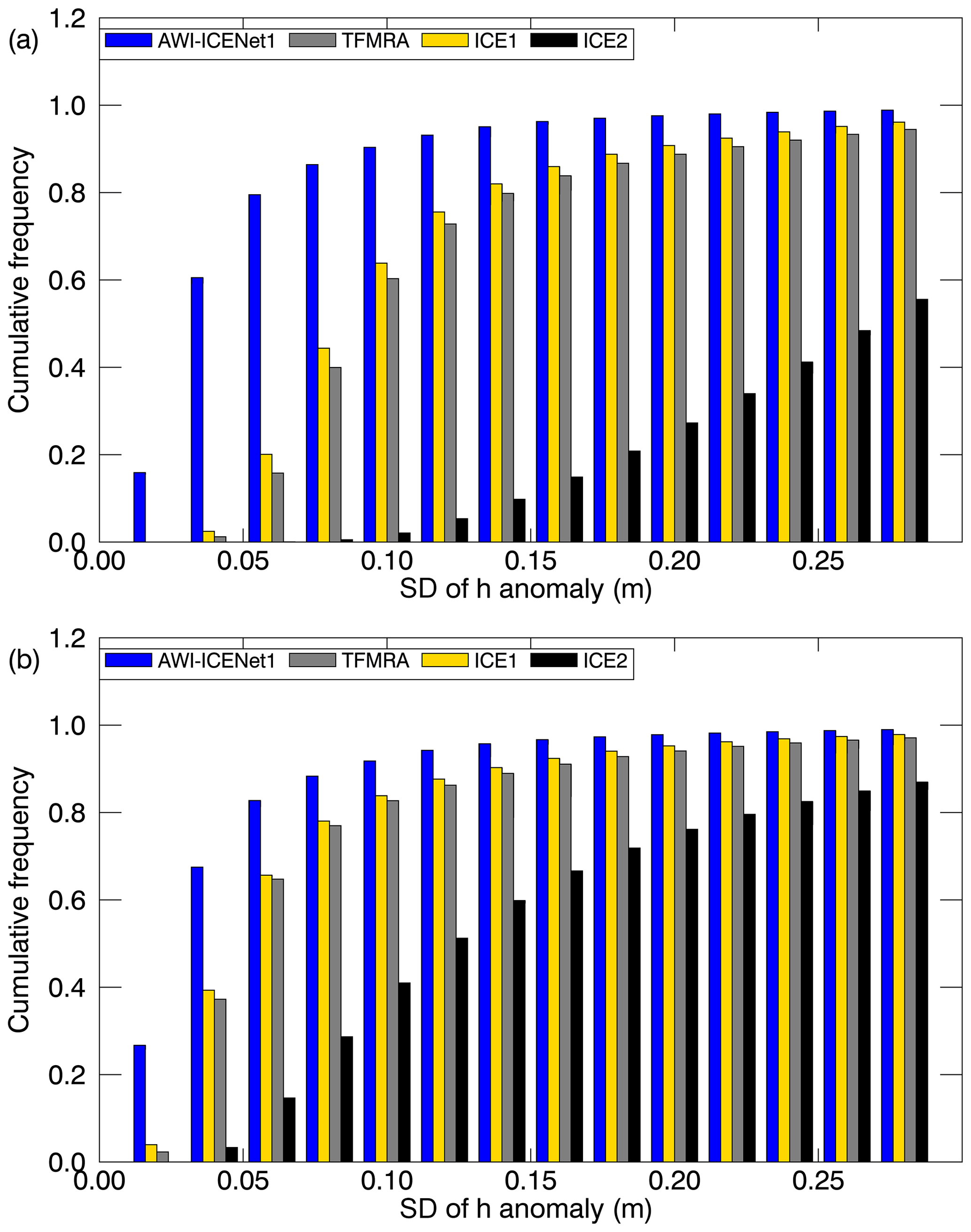
Figure 19Cumulative histogram (with a bin size of 0.02 m) illustrating the standard deviation of the elevation anomalies across the LRM zone in Antarctica for all four retrackers. (a) Uncorrected and (b) corrected h anomalies using correlations with LEW and backscatter. The elevation anomalies are based on grids with a 5 km × 5 km pixel resolution, derived from the spatially interpolated monthly residuals of the elevation trend estimation. The standard deviation is determined for each pixel across the full time period from January 2011 to December 2022.
4.1 Assessment of AWI-ICENet1 for simulated waveforms
Several waveform models have been developed to study the effects of physical parameters on waveform shape and their impact on retracked surface height, such as those by Ridley and Partington (1988), Femenias et al. (1993), Legrésy and Rémy (1997), Adams and Brown (1998), and Arthern et al. (2001). Martin et al. (1983) showed that the shape of the waveform's echo is affected by large-scale surface undulations. The surface slope has a large effect on the width of the leading edge (Femenias et al., 1993). Femenias et al. (1993) also showed that the error in the range retrieval due to volume backscatter can be up to 50 cm and mainly affects the trailing edge of the echo. Small-scale roughness can account for ±2 cm of the height bias. Our waveform model captures large-scale undulations and surface slope because we use a subset of the REMA as input for each simulated waveform. We do not consider macro roughness (metre-scale sastrugi) and small-scale roughness (centimetre-scale ripples) as these are not the main sources of error in height estimates. The sub-surface signal can be attenuated by various physical processes and parameters (e.g. absorption losses, scattering from ice grains, and multiple reflections within the snowpack caused by the stratification of the sub-surface due to density contrasts (Ridley and Partington, 1988; Femenias et al., 1993; Legrésy and Rémy, 1997)). In our model, we do not resolve the various parameters but consider their combined attenuation effect as an overall or bulk attenuation rate that changes the waveform. In Sect. 3.1, simulated sample waveforms for high and low LA are shown in Fig. 6. In addition to the significant difference in the TES, the broadening of the LEW for low LA is striking and reflects the observations of Femenias et al. (1993). This leads to incorrect estimates of TFMRA-retracked surface elevation as the retracked range is estimated to be 25 % of the leading edge (Helm et al., 2014). As a result, the retracked range is estimated within the first metre of the snowpack, depending on the width of the leading edge, rather than at the true surface, which is shown in Fig. 7. In contrast, AWI-ICENet1 strongly suppresses this penetration effect and positions the retracked range much closer to the true surface, making it less sensitive to errors caused by changes in the volume scattering contribution. Because AWI-ICENet1 has only been trained across the LRM zone, it may not be optimally trained for the very complex regions near the ice sheet margins. This could lead to larger errors when applied to pseudo-low-resolution-mode (PLRM) data included in the ESA Baseline-E data product. If AWI-ICENet1 were to be used for other missions (such as Envisat, SARAL/AltiKa, or Sentinel-3 (PLRM)), new simulations and training would be required to accurately represent mission-specific sensor characteristics, such as centre frequency, bandwidth, and antenna gain pattern.
4.2 Assessment of AWI-ICENet1 for satellite altimetry data
4.2.1 Cross-point-error analysis
In Sect. 3.2.1, CPE results were presented as the pan-Antarctic gridded median and SD values of the CPEs (Figs. 11 and 12). A prominent feature in the central part of East Antarctica (around the pole gap) was identified as a static crossover pattern. This pattern was described by Armitage et al. (2014) as the result of an isotropic dependence of the extinction coefficient on the angle between the radar polarization and wind-induced properties of the firn. In response to the Armitage et al. (2014) results, Box1 and Box2 were selected to investigate whether the crossover pattern is static over time and can be reduced using AWI-ICENet1. We have shown that the results for this area reveal a reduction in the CPE of about a factor of 4 for ICE1 and the TFMRA compared to ICE2 (note the different range of values in panel (c) of Fig. 11). A similar observation was made by Helm et al. (2014), in which the TFMRA showed slightly better results than the ESA ICE1 retracker. This finding is confirmed here as well. Moreover, the pattern is completely eliminated when using AWI-ICENet1, as displayed in panel (a) of Fig. 11. We conclude that the new AWI-ICENet1 retracker significantly suppresses the influence of the anisotropic dependence of the extinction coefficient and wind-driven directional anisotropy of the ice sheet surface and firn on surface height measurements, as described by Legresy et al. (1999). These results are consistent with those of Arthern et al. (2001), who found that the extinction coefficient (or, as we refer to it, the bulk attenuation rate) decorrelates between ascending and descending tracks. Because AWI-ICENet1 is able to minimize the effect of the bulk attenuation rate on range measurements, it is also able to remove the directional effect from ice sheet height measurements.
4.2.2 Transient penetration
Time-dependent elevation anomalies measured by radar satellite altimetry make up a composite signal of ice dynamical processes, changes in surface mass balance (SMB), changes in the firn compaction rate, and time-dependent radar penetration. In areas with low accumulation rates, such as the majority of the vast East Antarctic Ice Sheet, the latter can surpass SMB and firn compaction anomalies by 1 order of magnitude. To reliably estimate volume and mass changes, it is very important to correct for penetration bias as true elevation changes are only driven by changes in SMB, firn compaction, and ice dynamics. In Sect. 3.2.2, time-dependent variability in the elevation anomalies across the Lake Vostok area was presented. All retrackers usually used over ice sheets show surface height undulations of a couple of decimetres in areas known to be stable over recent decades (Richter et al., 2014). Similar findings for this area have been discussed in the literature regarding CryoSat-2 and Envisat, with methods proposed to partly suppress the penetration bias. As these undulations are driven by time-dependent changes in firn properties, a widely accepted method involves using the correlation between Δ h and backscatter and/or the waveform parameters (LEW and the TES), which are also affected by firn properties and thus change over time.
We applied this correction to all retrackers discussed in Sect. 3.2.2 and demonstrated its effectiveness. However, it is still unclear how much penetration bias contributes to the measured anomaly and how effectively the applied corrections can mitigate this bias. To address this issue, we compare our results with ICESat-2 observations and focus on the time period from January 2019 to December 2021, when both mission were in operation. Although ICESat-2 is a green-laser altimeter, a negligible penetration bias in dry snow can be assumed (Studinger et al., 2024). This is supported by and illustrated in Fig. 20, which shows the Δ h values observed by ICESat-2 in the given time period. In approximately 90 % of the area, the SD of Δ h is less than 0.04 m, indicating that for most of the area there is little variation in penetration, SMB, and/or firn compaction. Only in the Amundsen Sea Embayment (ASE) and along the Siple Coast in West Antarctica are h anomalies of more than 0.1 m found. The latter could indicate a dynamic thickening signal from the stagnant Kamb Ice Stream (Nield et al., 2016). The higher variability observed in the ASE can be explained by the extreme precipitation events that occurred in this area during the winters of 2019 and 2020, as reported by Davison et al. (2023). In Fig. 21, we compare the cumulative frequency of SD(Δ h) with ICESat-2 with regard to the uncorrected and corrected data in panels (a) and (b), respectively. AWI-ICENet1 already shows very close agreement with ICESat-2, even without any corrections, with only slight improvements observed when corrections are applied. However, for the TFMRA and ESA ICE1 retracker, the applied correction is very effective, although remaining signals are still present. The correction is not able to reduce SD(Δ h) to less than 4 cm, with only 30 % of the area for the TFMRA and ESA ICE1 retracker meeting this criterion (compared to 60 % for ICESat-2 and AWI-ICENet1). Our results illustrate that while backscatter and LEW corrections, even when applied over a relatively short time span of 3 years, significantly improve the data, they are not able to fully correct for erroneous signal contributions due to radar penetration. For longer time series, as shown in Fig. 19, the effect of the correction on ice-sheet-wide observations is even smaller.
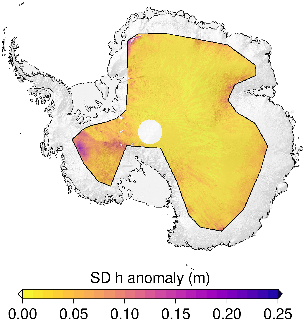
Figure 20ICESat-2-derived spatial distribution of the standard deviation of the elevation anomalies across the LRM zone in Antarctica. The elevation anomalies are based on grids with a 5 km × 5 km pixel resolution, derived from the spatially interpolated monthly residuals of the elevation trend estimation. The standard deviation is determined for each pixel across the time period from January 2019 to December 2021.
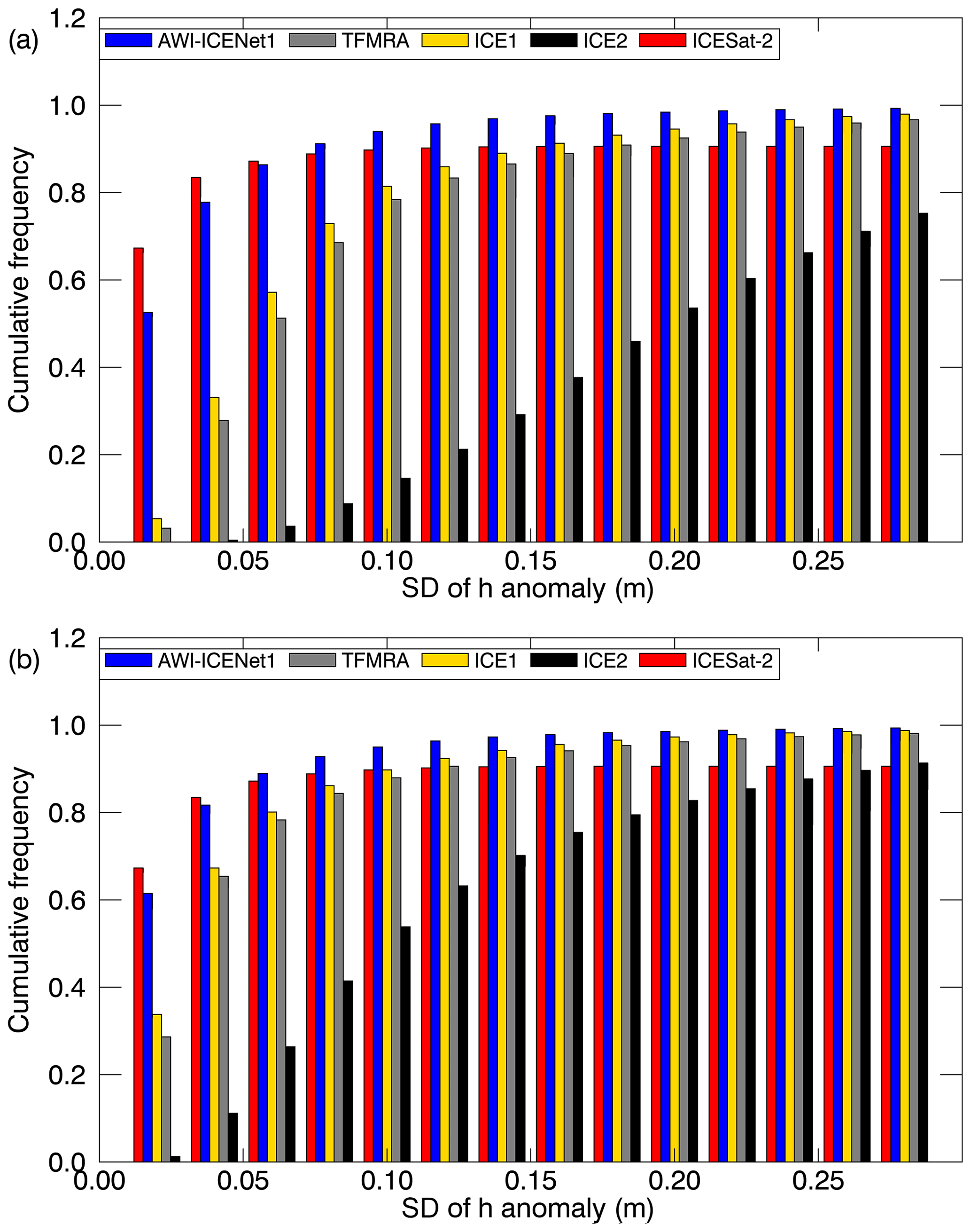
Figure 21Cumulative histogram (with a bin size of 0.02 m) illustrating the standard deviation of the elevation anomalies across the LRM zone in Antarctica for all four retrackers and ICESat-2. (a) Uncorrected and (b) corrected h anomalies using correlations with LEW and backscatter. The elevation anomalies are based on grids with a 5 km × 5 km pixel resolution, derived from the spatially interpolated monthly residuals of the elevation trend estimation. The standard deviation is determined for each pixel across the time period from January 2019 to December 2021.
4.2.3 Sudden changes in scattering properties and their effect on elevation change
Nilsson et al. (2015, 2016), McMillan et al. (2016), and Simonsen and Sørensen (2017) discussed the unusual melt event that occurred across the Greenland Ice Sheet in July 2012 and analysed its impact on CryoSat-2 observations. Nilsson et al. (2015) reported improved performance using a 20 % threshold retracker for LRM data, which showed reduced sensitivity to changes in near-surface scattering properties. This result is in close agreement with the findings of Helm et al. (2014). On the other hand, McMillan et al. (2016) introduced a step function to mitigate the observed elevation step. This procedure however, is not applicable as a general approach as it cannot account for multiple melt events, which can be expected in future. Using the “LRM_L2” data from the ESA, Simonsen and Sørensen (2017) studied the impact of different waveform parameters (LEW and backscatter) in correcting for scattering properties in CryoSat-2 observations for the time span from November 2010 to November 2014. Their findings suggest that LEW correction is the most effective approach for the LRM zone. They also found that some bias in temporal changes is not entirely removed, which aligns with our results for the ESA ICE1 and ICE2 retrackers. In order to evaluate whether AWI-ICENet1 is capable of handling sudden scattering changes, we applied processing to all retrackers for the time span from January 2011 to December 2014, covering nearly the same period investigated by Simonsen and Sørensen (2017). In Fig. 22, uncorrected values are shown, and in Fig. A17, values corrected using LEW and backscatter are shown. The same unusual elevation increase, with mean rates of 0.1–0.2 m yr−1, is observed for the ESA ICE1 retracker and TFMRA across large parts of the highly elevated area. The ESA ICE2 retracker shows rates of >0.25 m yr−1 for almost the entire LRM zone. Only the southeastern part experiences surface lowering. In contrast, AWI-ICENet1-derived ranges from -0.05 to 0.05 m yr−1 and does not seem affected by the change in scattering characteristics due to the surface melt event. When compared to the corrected estimates, we find the best agreement with the ESA ICE1 retracker and TFMRA. In agreement with Simonsen and Sørensen (2017), we find that the corrected TFMRA and the ESA ICE1 and ICE2 retrackers still show some remaining signal. The application of a low-threshold retracker, as suggested by Nilsson et al. (2015), strongly reduces sensitivity to scattering changes, but it still needs to be combined with waveform parameter corrections to provide reliable results. Only AWI-ICENet1 incorporates most of the correction directly within the retracking process. The differences between uncorrected and corrected estimates are within the uncertainty of 8 km3 yr−1, as listed in Table 3. AWI-ICENet1 is in close agreement with the LEW estimates from the ESA ICE1 retracker. These have been found to match best with surface elevation changes measured by lidar during the Operation IceBridge campaigns, as presented by Simonsen and Sørensen (2017), and agree well with our corrected TFMRA estimates.
Table 3Volume change estimates for Greenland for the period from January 2011 to December 2014, derived using different retrackers and corrections. All values are given in km3 yr−1.
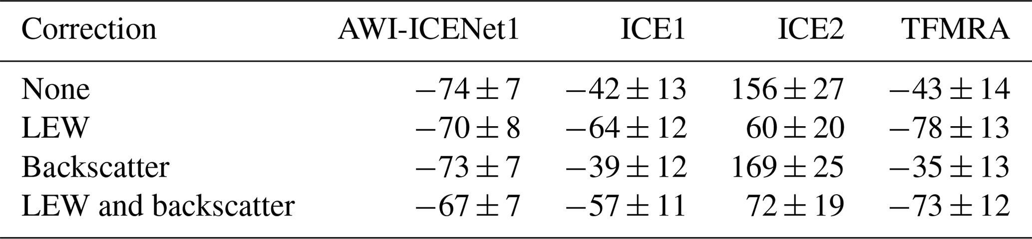

Figure 22Greenland-wide estimates from four retrackers for the period from January 2011 to December 2013, which includes the July melt event of 2012.
4.2.4 Comparison of elevation change estimates with ICESat-2 data
To further assess the performance of the retrackers, we conduct a comparison between elevation change () and ICESat-2 data for the time span from January 2019 to December 2021. The difference in elevation change ( for CryoSat-2 – for ICESat-2), i.e. the difference, is displayed in Fig. 23 for each retracker individually. Again, the patterns for the ESA ICE1 retracker and TFMRA are similar spatially as well as in terms of magnitude. The ESA ICE2 retracker deviates the most from the ICESat-2 elevation change. The new AWI-ICENet1 shows deviations of less than ±0.1 m yr−1 from ICESat-2 over approximately 90 % of the entire area. Table 4 lists estimated volume changes () observed in the LRM zone for the time span from January 2019 to December 2021 for ICESat-2 and all retrackers that include the applied corrections for both ice sheets. In Antarctica, the difference between applying and not applying the correction is tremendously high for ICE2, ranging from 84 to 276 km3 yr−1, followed by the TFMRA (a range of 72 km3 yr−1) and the ESA ICE1 retracker (a range of 56 km3 yr−1). AWI-ICENet1 shows the smallest range, only 9 km3 yr−1, indicating that most of the corrections are already covered by the retracker itself. The results also show the necessity of applying the corrections to all retrackers except AWI-ICENet1; otherwise, and, consequently, mass balance estimates are unreliable, particularly for East Antarctica. The uncorrected estimates are prone to errors which are strongly related to elevation anomalies originating from changes in the electromagnetic properties of the upper layers of the snow/firn pack. In Greenland, the same conclusion can be drawn. Here, the spread of is smaller. The spread is 41 km3 yr−1 for the ESA ICE2 retracker, 8 km3 yr−1 for the ESA ICE1 retracker, 6 km3 yr−1 for the TFMRA, and only 4 km3 yr−1 for AWI-ICENet1. In all cases, the uncertainty in the estimates could be reduced using the combined correction of LEW and backscatter. The smallest spread between the different retracker solutions is also found using LEW and backscatter corrections applied across Antarctica and Greenland, respectively. Interestingly, as shown in Figs. 15, 18, A11, and A12, none of the corrections applied to the ESA ICE1 and ICE2 retrackers and the TFMRA are capable of reducing Δ h as effectively as AWI-ICENet1. This is particularly evident for Greenland, as shown in Table 4, where none of the estimates reach values of 5 km3 yr−1, as observed by ICESat-2. For Greenland and Antarctica, AWI-ICENet1 also reveals the smallest offsets compared to ICESat-2; in both cases, the difference in is less than 20 km3 yr−1, where ICESat-2 tends to show larger values (compared to those displayed in panel (a) of Figs. 23, 24, A15, and A16). This small (<1 cm yr−1) difference in compared to ICESat-2 is most likely a residual signal due to radar penetration and thus not related to any ICESat-2 mission bias, as observed for the predecessor mission ICESat-1 (NSIDC, 2021). Sea level trends computed from ICESat-2 observations agree with independent measurements from radar altimetry and tide gauges, as shown by Buzzanga et al. (2021), and do not indicate any trend bias (at least over oceans). In Antarctica, the best match with AWI-ICENet1 is found for the TFMRA with LEW and backscatter corrections applied. In Figs. A5, A6, A7, and A8, the correlations between the elevation anomalies and LEW, as well as those between the elevation anomalies and backscatter, are shown. For AWI-ICENet1, the correlations are lower than for the other three retrackers, but this is expected since the h anomalies are already strongly suppressed by AWI-ICENet1, which should lead to much lower correlations with backscatter or LEW. In particular, the correction with backscatter needs to be carefully checked as it can introduce errors which most likely originate from errors in the power scaling factors applied to the Level 1B LRM data, as reported by the ESA (Exprivia, 2021). This issue caused the backscatter computed at Level 1 to differ between the Baseline-D and Baseline-E products, resulting in a jump in backscatter in August 2019 when the Baseline-E product was operational (Exprivia, 2021). The issue was solved in the reprocessed Baseline-E data. In our processing, we used this reprocessed Baseline-E data and thus do not expect any issues with the backscatter.
Table 4Volume change estimates for Greenland (GRE) and Antarctica (ANT) for the period from January 2019 to December 2021, derived using different retrackers compared to ICESat-2. All values are given in km3 yr−1.
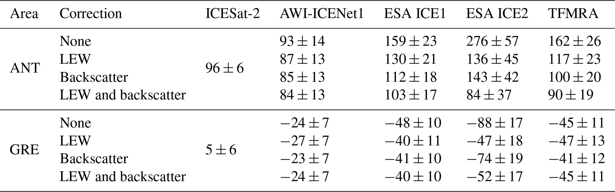
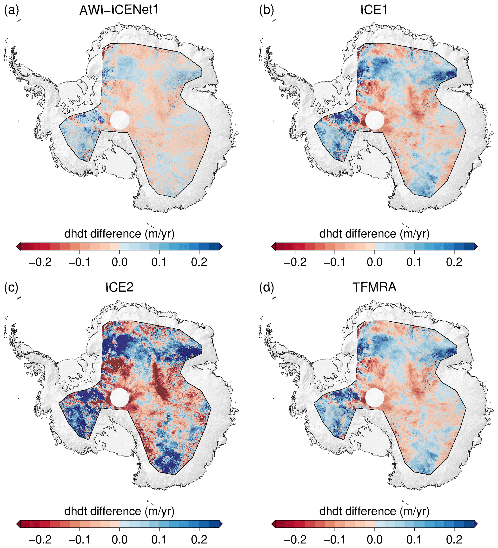
Figure 23Antarctic-wide difference from ICESat-2 for four retrackers for the period from January 2019 to December 2021.
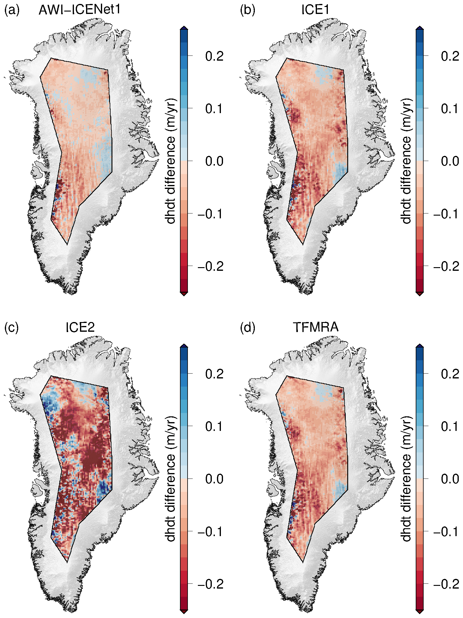
Figure 24Greenland-wide difference from ICESat-2 for four retrackers for the period from January 2019 to December 2021.
4.2.5 Computational performance
Unlike many other machine learning applications used in remote sensing, AWI-ICENet1 was not designed to replace manual labour or save time but to improve observation quality. In fact, our computational-performance test results, shown in Table 2, highlight that AWI-ICENet1 requires more processing time than conventional empirical retracking methods. In particular, AWI-ICENet1 requires about 8 times more computing time than the TFMRA and around 18 times more than the TCOG retracker, both of which are cheap empirical retracking methods with low computing costs. However, if the estimation of the LEW is also taken into account in the TCOG retracker and TFMRA, the difference in processing time compared to that of the AWI-ICENet1 is considerably reduced. Therefore, we do not consider the higher computational cost of AWI-ICENet1 to be a significant drawback for its use, regardless of the computing infrastructure. Compared to more complicated waveform-fitting methods based on analytical descriptions of the waveform, such as classical ocean retrackers (e.g. the maximum likelihood estimators MLE3 and MLE4 (Amarouche et al., 2004; Thibaut et al., 2010), adaptive versions of MLE3 and MLE4 (Thibaut et al., 2021), SAMOSA+ (Dinardo et al., 2018), and SAMOSA++ (Dinardo et al., 2021)), ConvNet-based approaches are expected to help significantly reduce processing costs. Reprocessing campaigns could benefit from neural-network-based approaches. However, for each of the aforementioned the analytical retrackers, a specific ConvNet model that best represents the analytical solution would have to be trained in advance with a considerable number of waveforms covering the entire spectrum of possible waveforms.
We conclude that the use of AWI-ICENet1, a new retracker for ice altimetry based on a convolutional network, provides better performance in deriving ice-sheet-wide elevation products than currently used retrackers, such as the TFMRA or the ESA Level-2 ICE1 and ICE2 products. Across all terrain types, the performance of AWI-ICENet1 in terms of the CPE is similar to that of the ESA Level-2 ICE1 product, the highest-precision retracker. The main improvement with our new approach is the large reduction in sensitivity to transient signal penetration due to temporal changes in near-surface scattering properties of the firn in comparison to other approaches. The transient-penetration bias, which can be on the order of several decimetres, is reduced to a few centimetres by AWI-ICENet1. AWI-ICENet1 can handle abrupt changes in the prevailing scattering mechanism due to surface melt, such as those that occurred across Greenland in July 2012, as well as temperature-induced changes in the bulk attenuation rate of the upper firn layers, which are mainly observed as a seasonal signal in East Antarctica. The contribution of transient penetration to the measured elevation anomaly is greatly reduced compared to that of equivalent products, even when it is compared to empirically corrected data using a correlation between elevation changes and changes in backscatter or waveform shape parameters, such as LEW. This results in a much more accurate sampling of true elevation changes due to changes in SMB or firn compaction, and estimates agree well with ICESat-2-derived estimates that are not susceptible to transient penetration. Using the new retracking method for CryoSat-2 LRM data, we determine the volume change in the LRM zone of the Antarctic and Greenland ice sheets for the period from January 2019 to December 2021 to be 84±13 and km3 yr−1, respectively. This agrees well with ICESat-2 estimates obtained across both ice sheets during the same period (96±6 and 5±6 km3 yr−1). The improvements in our new retracking approach reduce the need for correlation corrections in post-processing, which can introduce additional bias as a result of anomalous backscatter variations caused by different processing baselines. In addition, empirical corrections are sensitive to the length of the time series used to apply the correction. The new retracking method provides higher intrinsic accuracy in the measured surface elevation and thus lower uncertainty in derived products, such as elevation change and volume change estimates. This will lead to an improved understanding of the response of ice sheets to climate change, especially with respect to areas of low elevation change, such as the East Antarctic Plateau, where high measurement accuracy is required to separate true elevation change from noise originating from transient radar penetration.
In the future, AWI-ICENet1 should also be applied to pulse-limited altimetry products (LRM and PLRM) from past (Envisat, ERS-1, and ERS-2), present (Sentinel-3A, Sentinel-3B, and SARAL/AltiKa), and future Copernicus Polar Ice and Snow Topography Altimeter (CRISTAL) altimetry missions to extend the time series and realize a consistent elevation change product with the fewest possible penetration-biased estimates. Furthermore, extending the waveform simulator to SAR waveforms would be highly valuable for applying a similar approach to CRISTAL and Sentinel-3 SAR data.
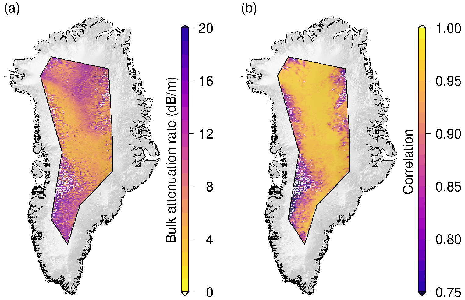
Figure A1Results of the test in which a flat-surface waveform model was fitted to real CryoSat-2 waveforms by adjusting the attenuation LA as the only parameter. (a) Gridded median of the attenuation rate estimated by an MLE fit. (b) Median of the correlation between the observed and fitted waveforms.
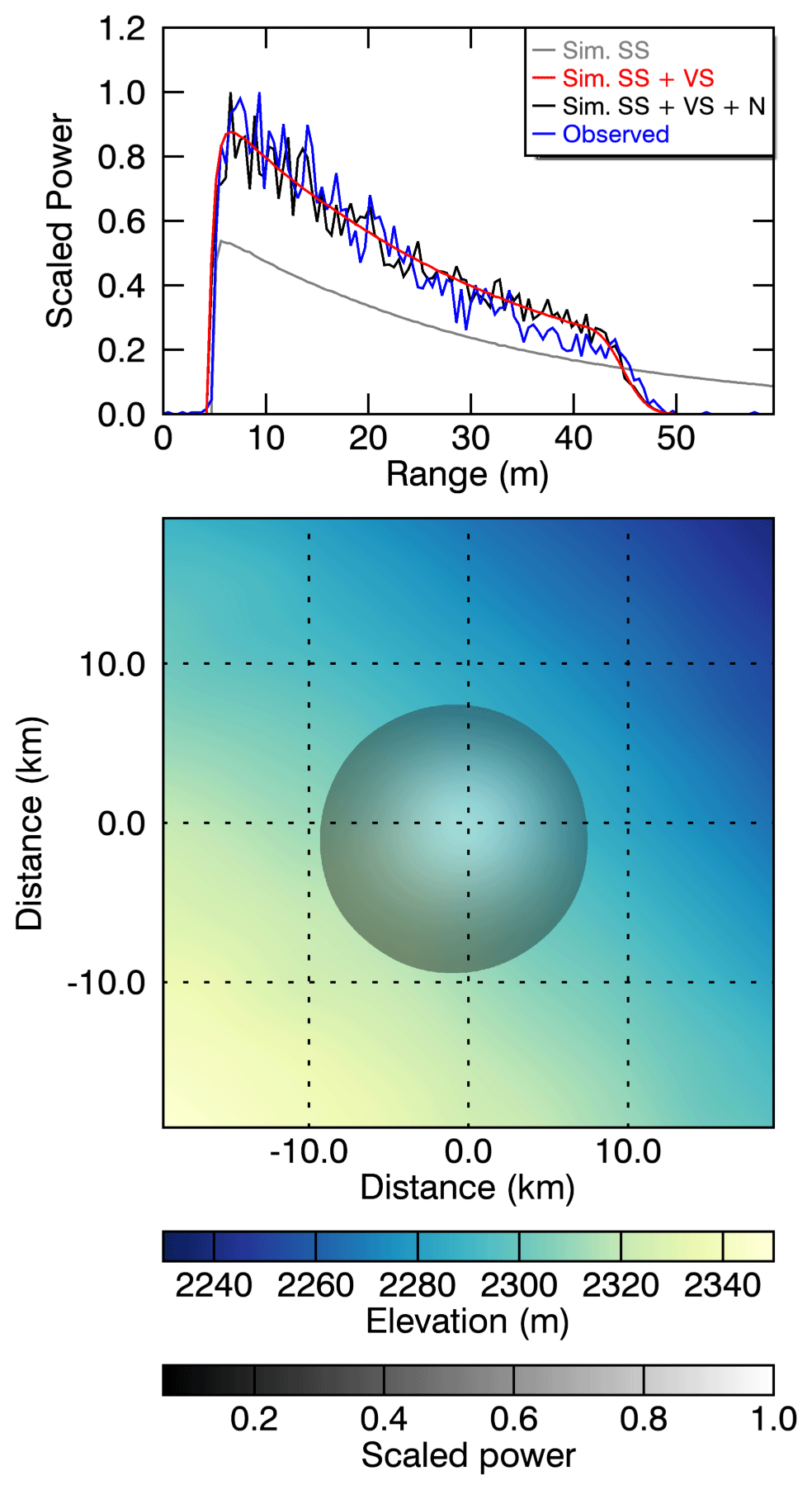
Figure A2Example of the different simulation steps for a typical waveform around the North Greenland Eemian Ice Drilling (NEEM) ice core site in Greenland. The blue line depicts the observed CryoSat-2 LRM waveform, and the grey line represents the simulated surface waveform based on Eq. (1). The red line indicates the simulated waveform with volume scattering, based on Eq. (3), while the black line displays the final simulated waveform, which includes surface and volume scattering as well as noise, as given in Eq. (5). The lower panel represents the 2D elevation model as well as scaled , which is mainly controlled by the Gaussian antenna pattern.
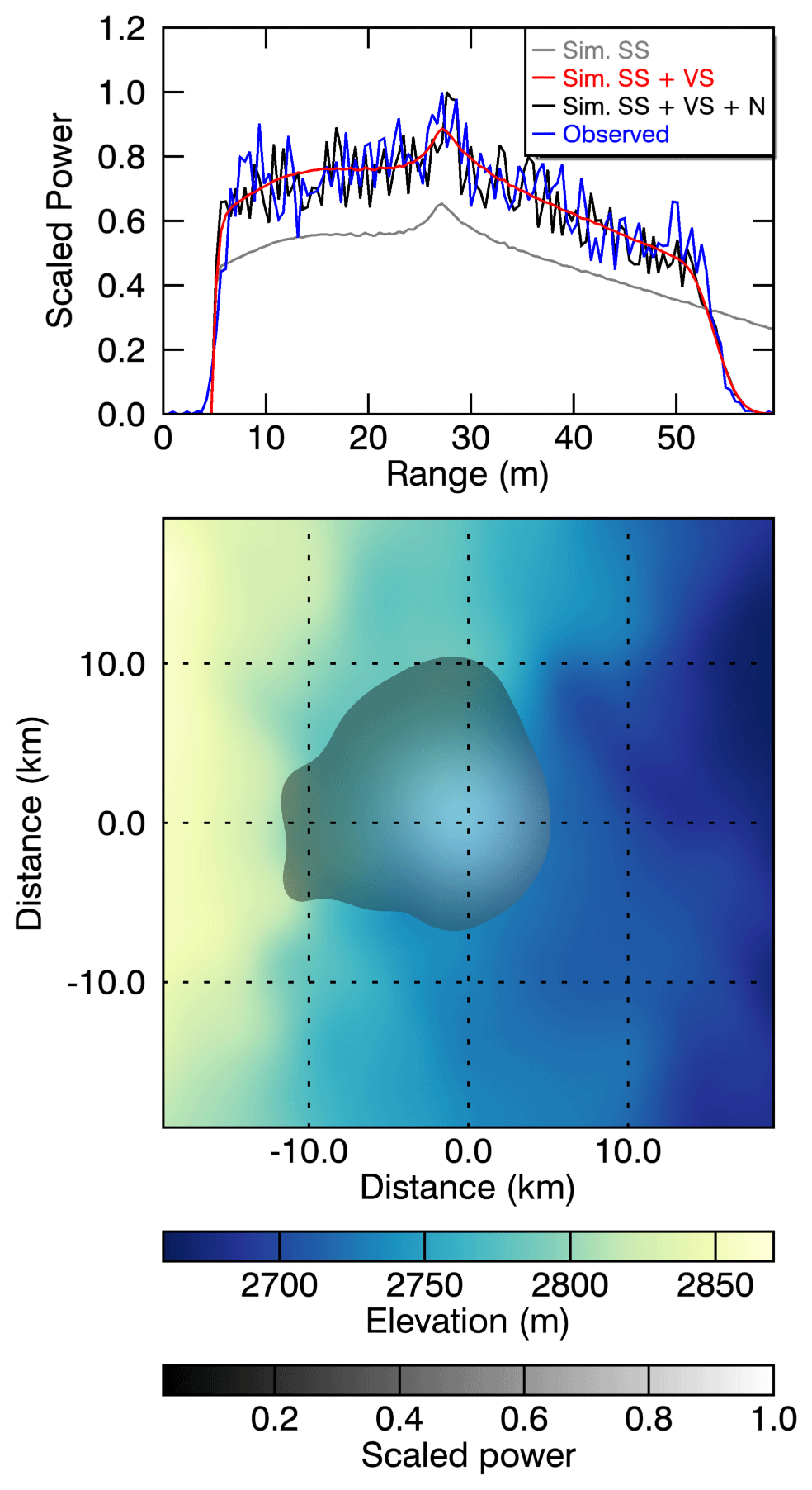
Figure A3Example of the different simulation steps for a typical waveform in the Amery drainage basin (region A in Fig. 1). The blue line depicts the observed CryoSat-2 LRM waveform, and the grey line represents the simulated surface waveform based on Eq. (1). The red line shows the simulated waveform with volume scattering, based on Eq. (3), while the black line displays the final simulated waveform, which includes surface and volume scattering as well as noise, as given in Eq. (5). The lower panel represents the 2D elevation model as well as scaled , which is mainly controlled by the Gaussian antenna pattern.
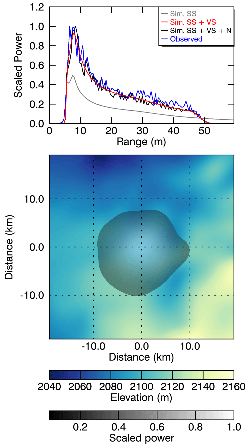
Figure A4Example of the different simulation steps for a typical waveform in the Recovery area (see Fig. 1). The blue line depicts the observed CryoSat-2 LRM waveform, and the grey line represents the simulated surface waveform based on Eq. (1). The red line depicts the simulated waveform with volume scattering, based on Eq. (3), while the black line displays the final simulated waveform, which includes surface and volume scattering as well as noise, as given in Eq. (5). The lower panel represents the 2D elevation model as well as scaled , which is mainly controlled by the Gaussian antenna pattern.
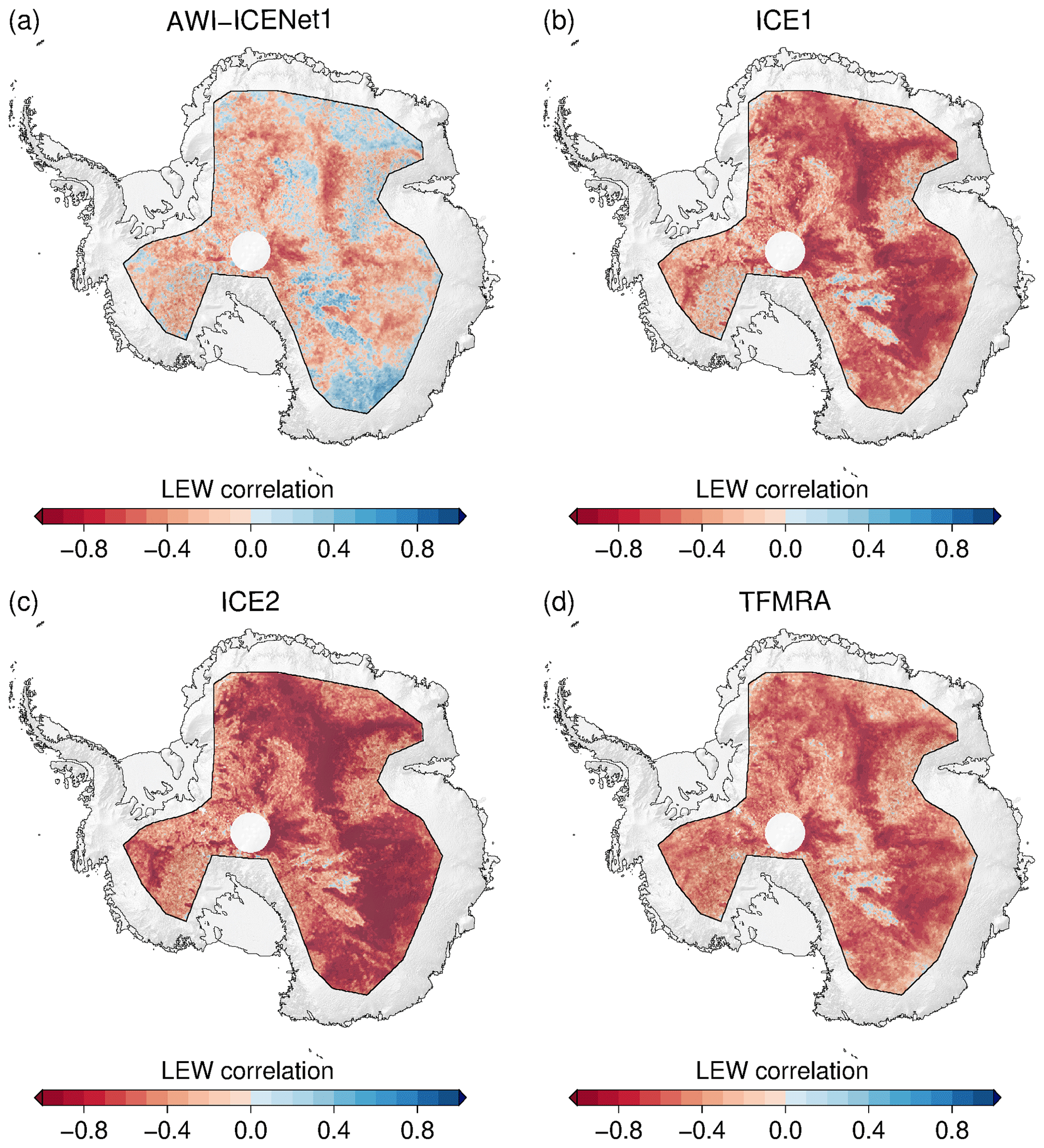
Figure A5Correlation between elevation anomalies and LEW for different retrackers across Antarctica. The correlation is based on the full time series from January 2011 to December 2022.
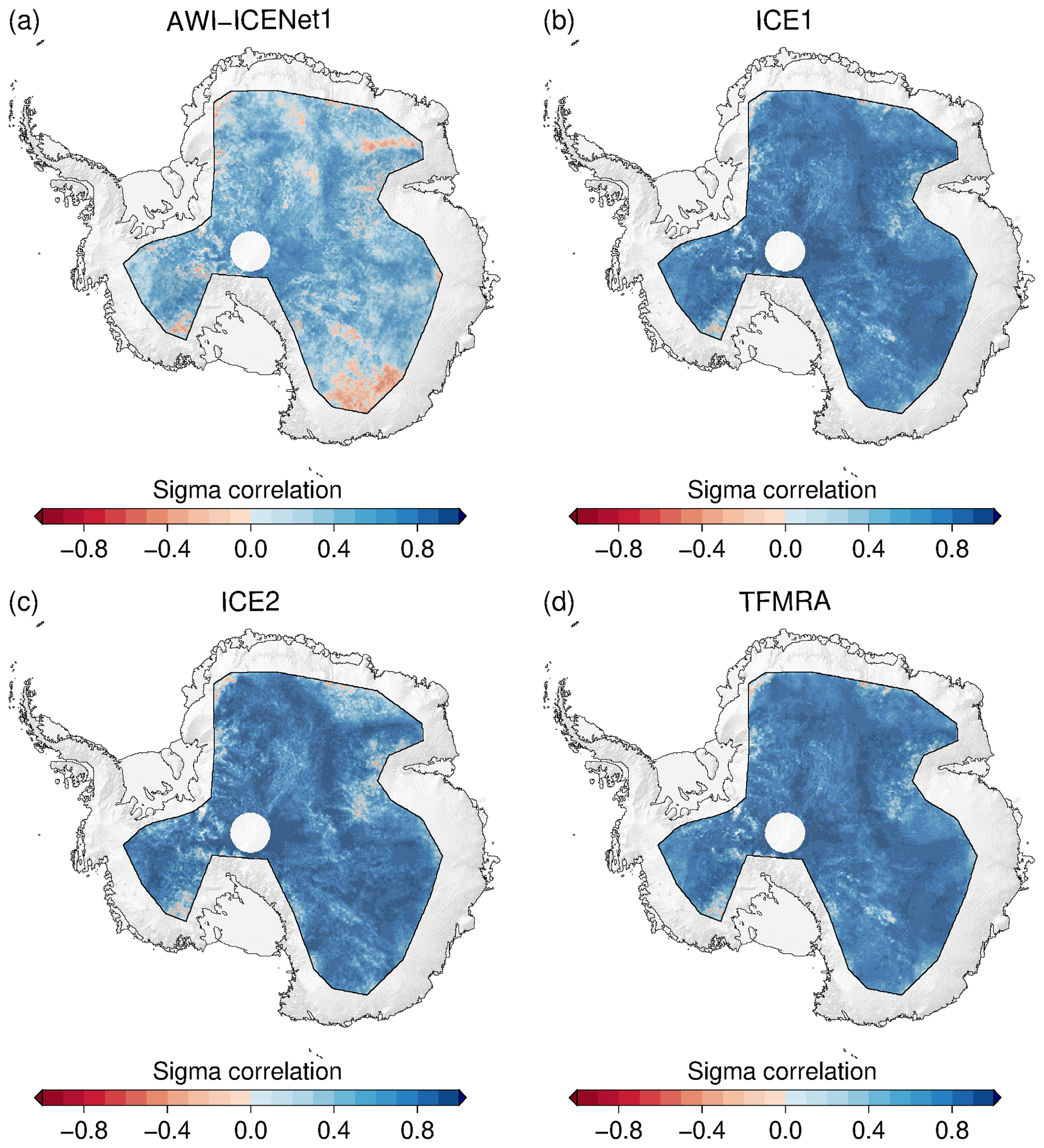
Figure A6Correlation between elevation anomalies and backscatter for different retrackers across Antarctica. The correlation is based on the full time series from January 2011 to December 2022.
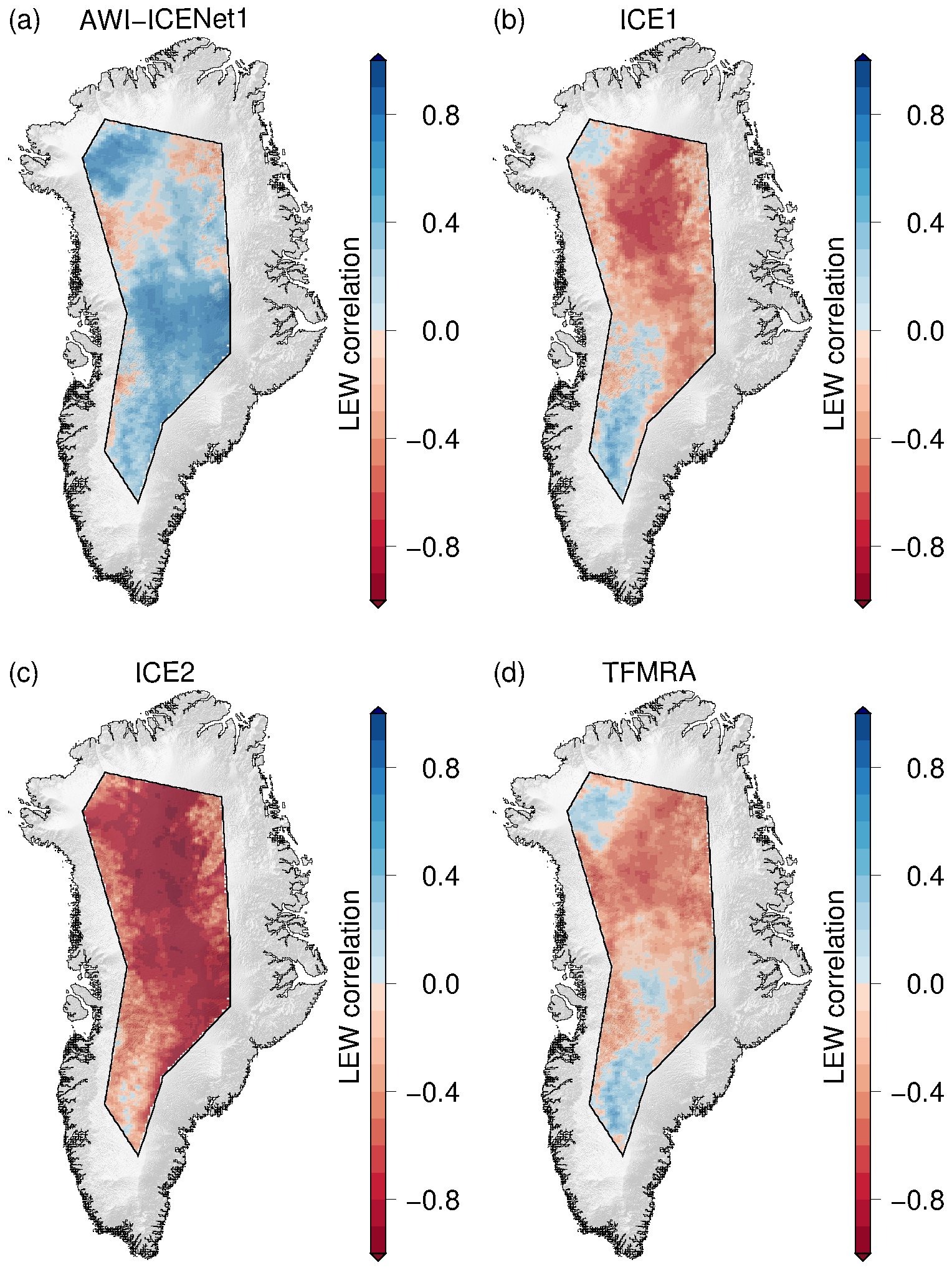
Figure A7Correlation between elevation anomalies and LEW for different retrackers across Greenland. The correlation is based on the full time series from January 2011 to December 2022.
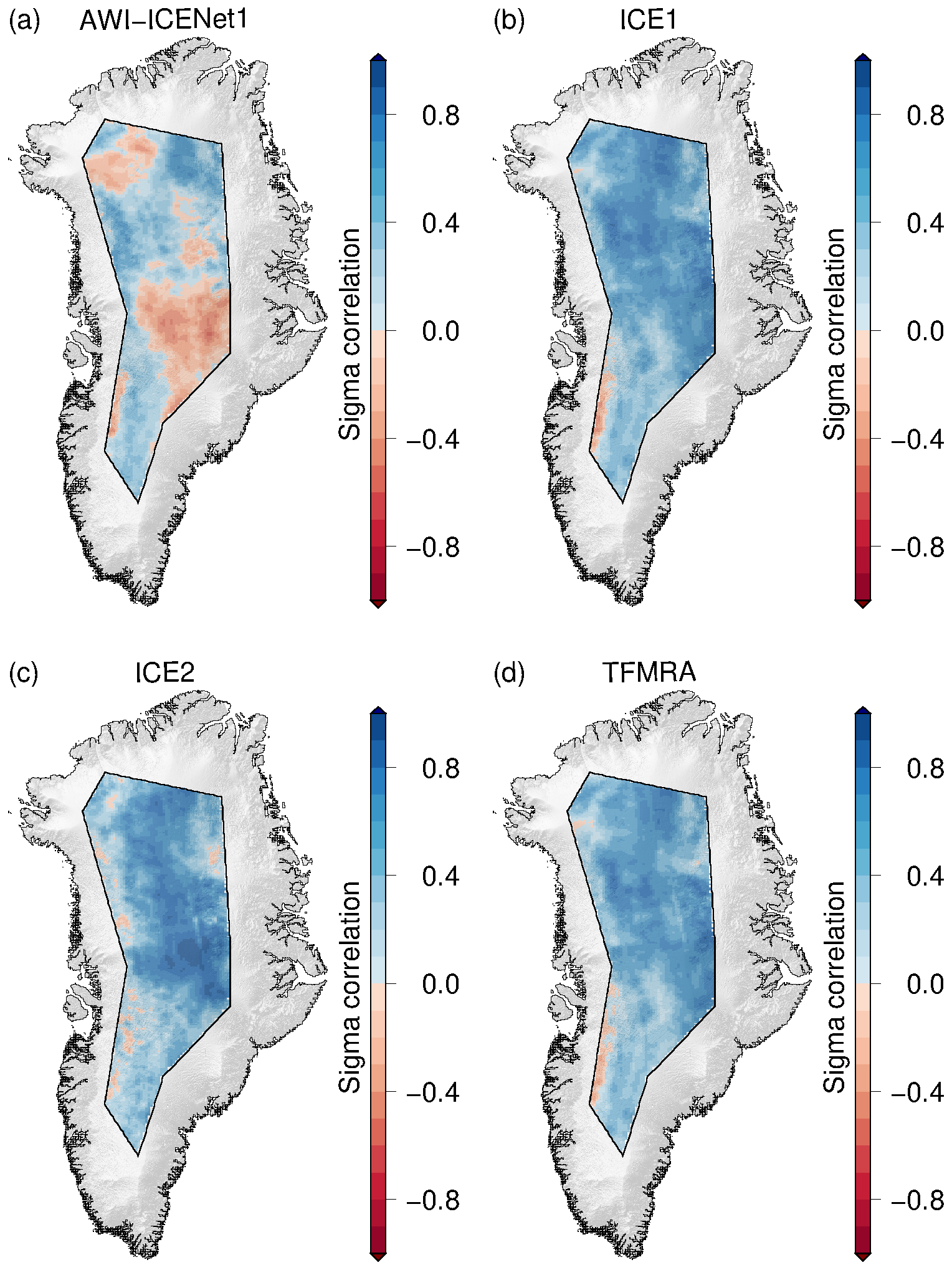
Figure A8Correlation between elevation anomalies and backscatter for different retrackers across Greenland. The correlation is based on the full time series from January 2011 to December 2022.
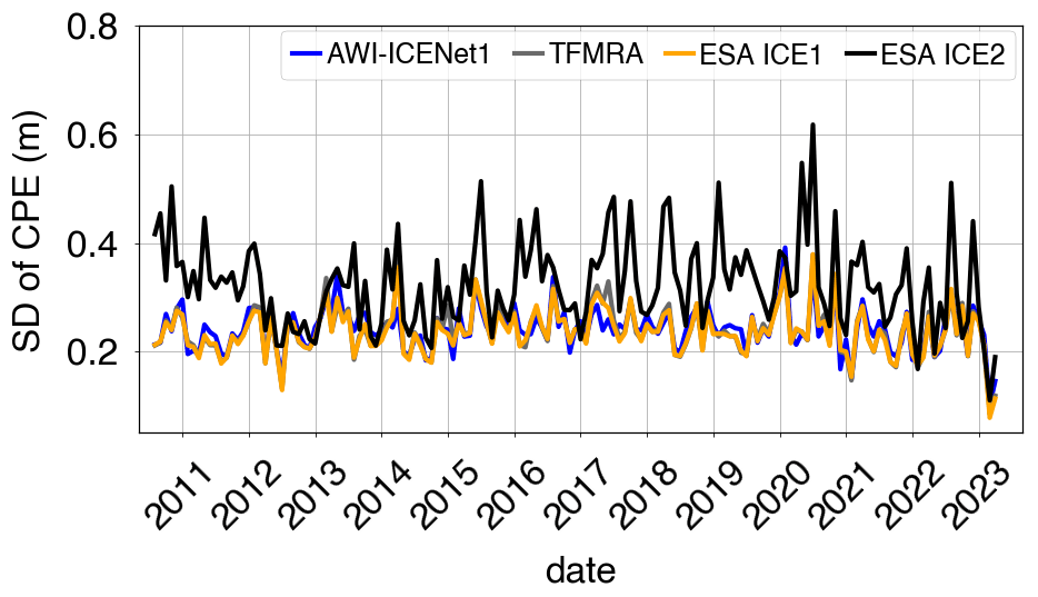
Figure A9Time series of the standard deviation of cross-point errors for a region in North Greenland. Cross-point errors are determined at a monthly resolution.
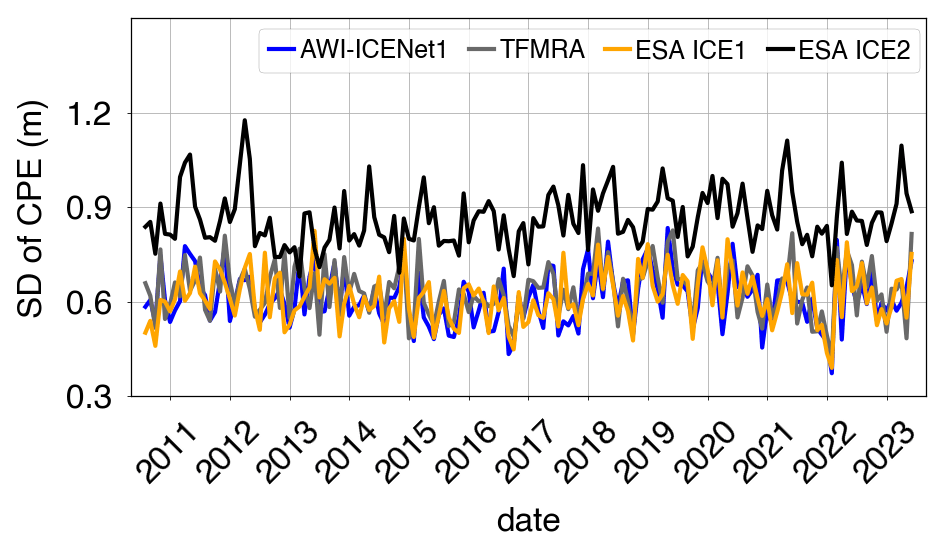
Figure A10Time series of the standard deviation of cross-point errors for the LRM zone in Greenland. Cross-point errors are determined at a monthly resolution.
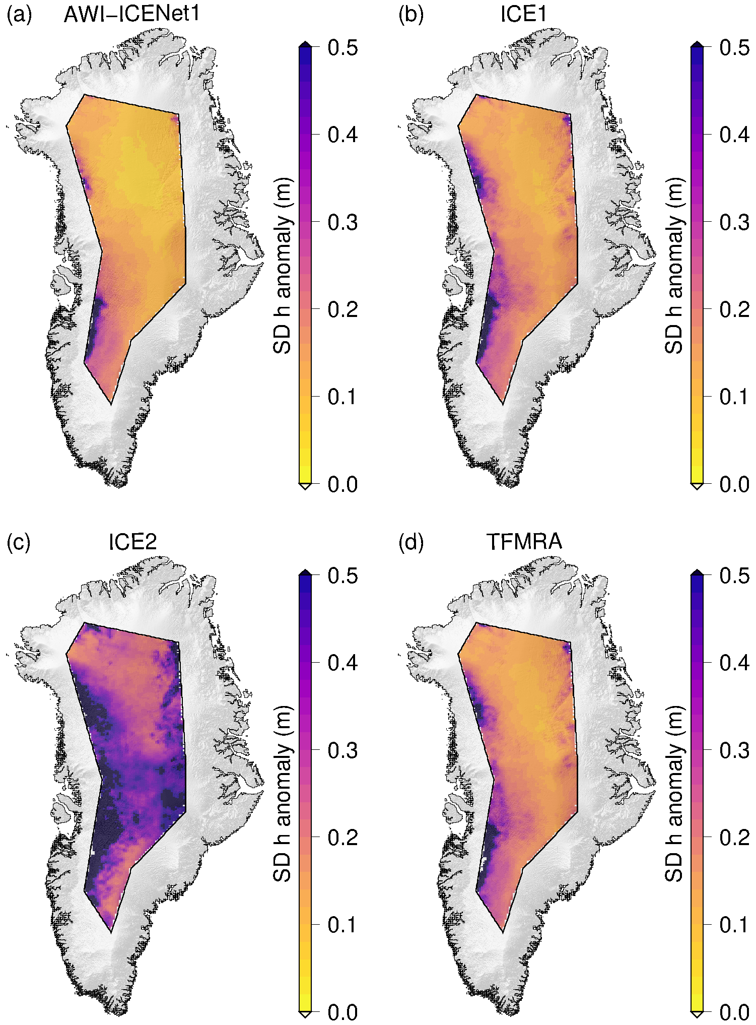
Figure A11Spatial distribution of the standard deviation of the elevation anomalies across the LRM zone in Greenland for all four retrackers. The elevation anomalies are based on grids with a 5 km × 5 km pixel resolution, derived from the spatially interpolated monthly residuals of the elevation trend estimation. The standard deviation is determined for each pixel across the full time period from January 2011 to December 2022.
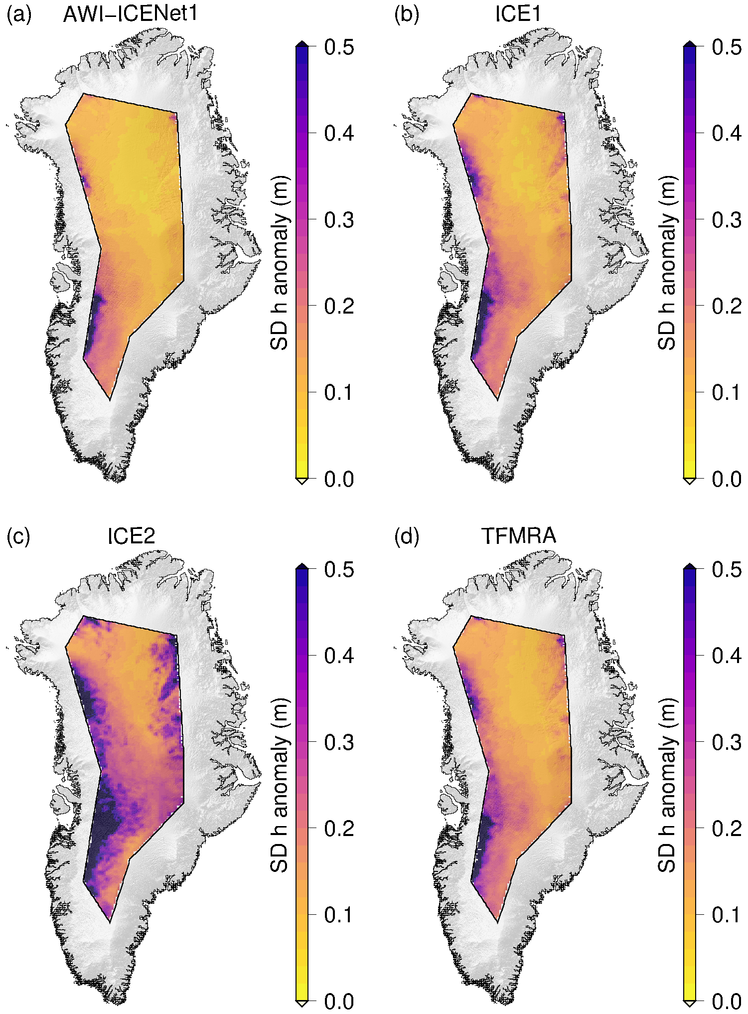
Figure A12Spatial distribution of the standard deviation of the corrected elevation anomaly across the LRM zone in Greenland for all four retrackers. The elevation anomalies are based on grids with a 5 km × 5 km pixel resolution, derived from the spatially interpolated monthly residuals of the elevation trend estimation that were corrected using correlations with leading-edge width and backscatter. The standard deviation is determined for each pixel across the full time period from January 2011 to December 2022.
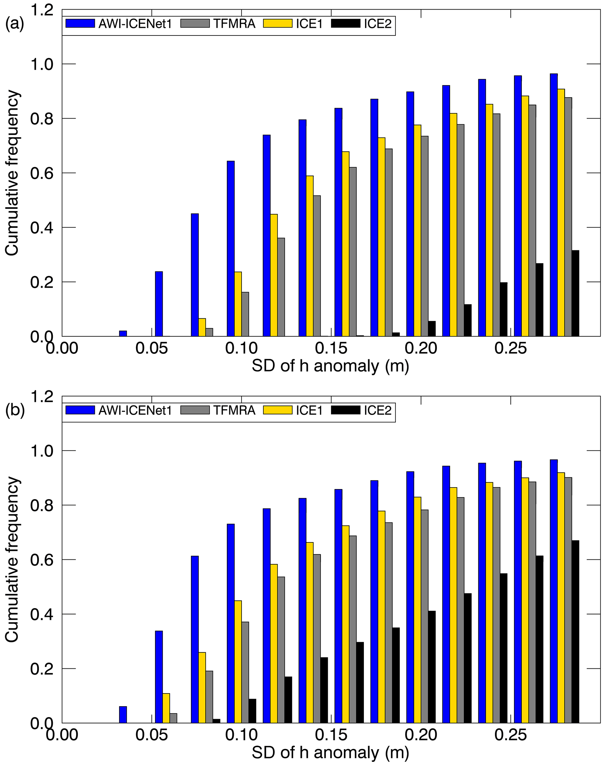
Figure A13Cumulative histogram (with a bin size of 0.02 m) illustrating the standard deviation of the elevation anomalies across the LRM zone in Greenland for all four retrackers. (a) Uncorrected and (b) corrected h anomalies using correlations with LEW and backscatter. The elevation anomalies are based on grids with a 5 km × 5 km pixel resolution, derived from the spatially interpolated monthly residuals of the elevation trend estimation. The standard deviation is determined for each pixel across the full time period from January 2011 to December 2022.
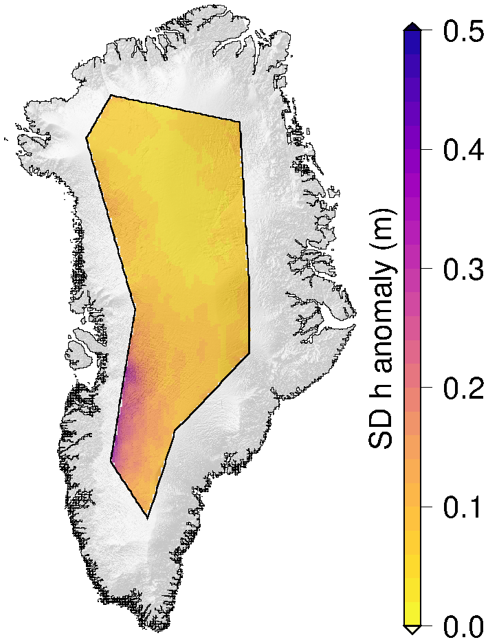
Figure A14ICESat-2-derived spatial distribution of the standard deviation of the elevation anomalies across the LRM zone in Greenland. The elevation anomalies are based on grids with a 5 km × 5 km pixel resolution, derived from the spatially interpolated monthly residuals of the elevation trend estimation. The standard deviation is determined for each pixel across the time period from January 2019 to December 2021.
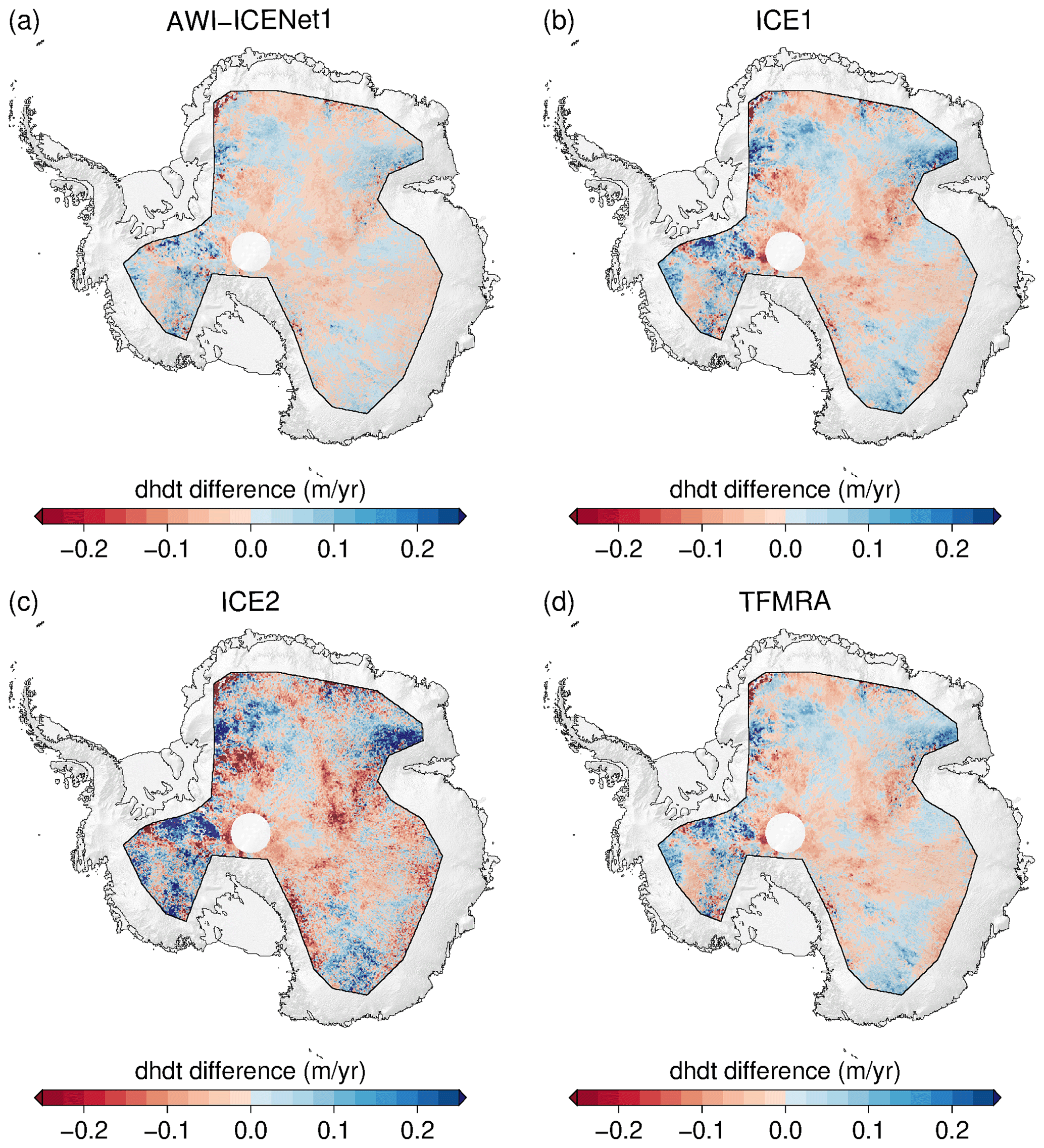
Figure A15Antarctic-wide difference from ICESat-2 for four retrackers for the period from January 2019 to December 2021, including LEW and backscatter correction.
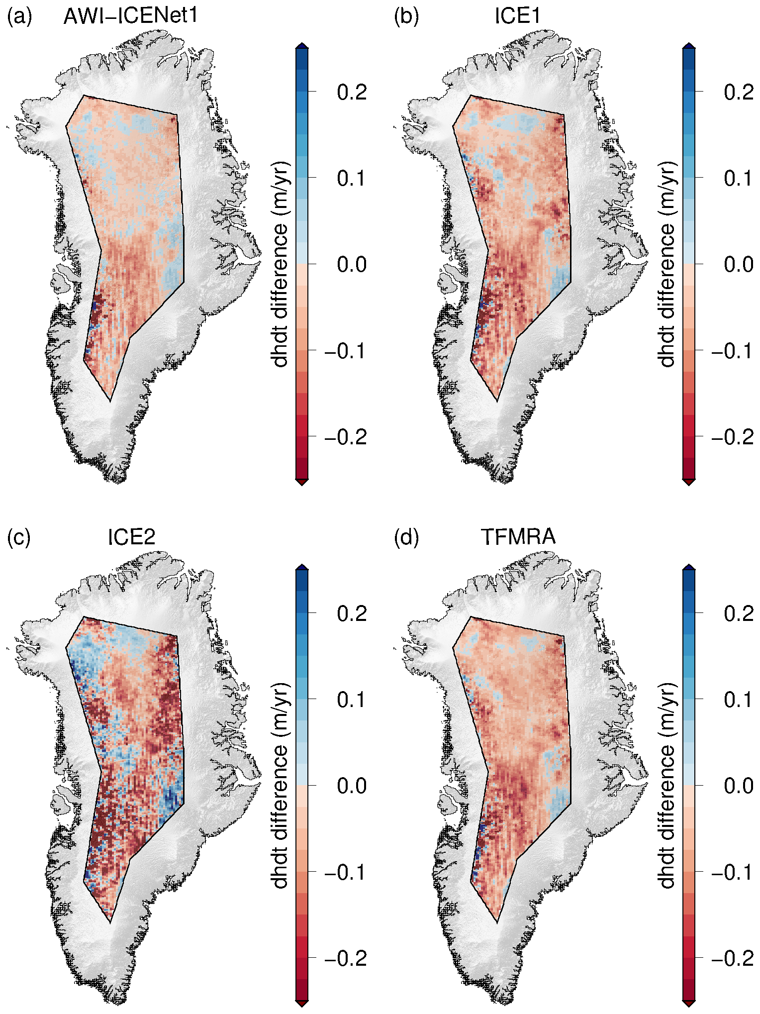
Figure A16Greenland-wide difference from ICESat-2 for four retrackers for the period from January 2019 to December 2021, including LEW and backscatter correction.
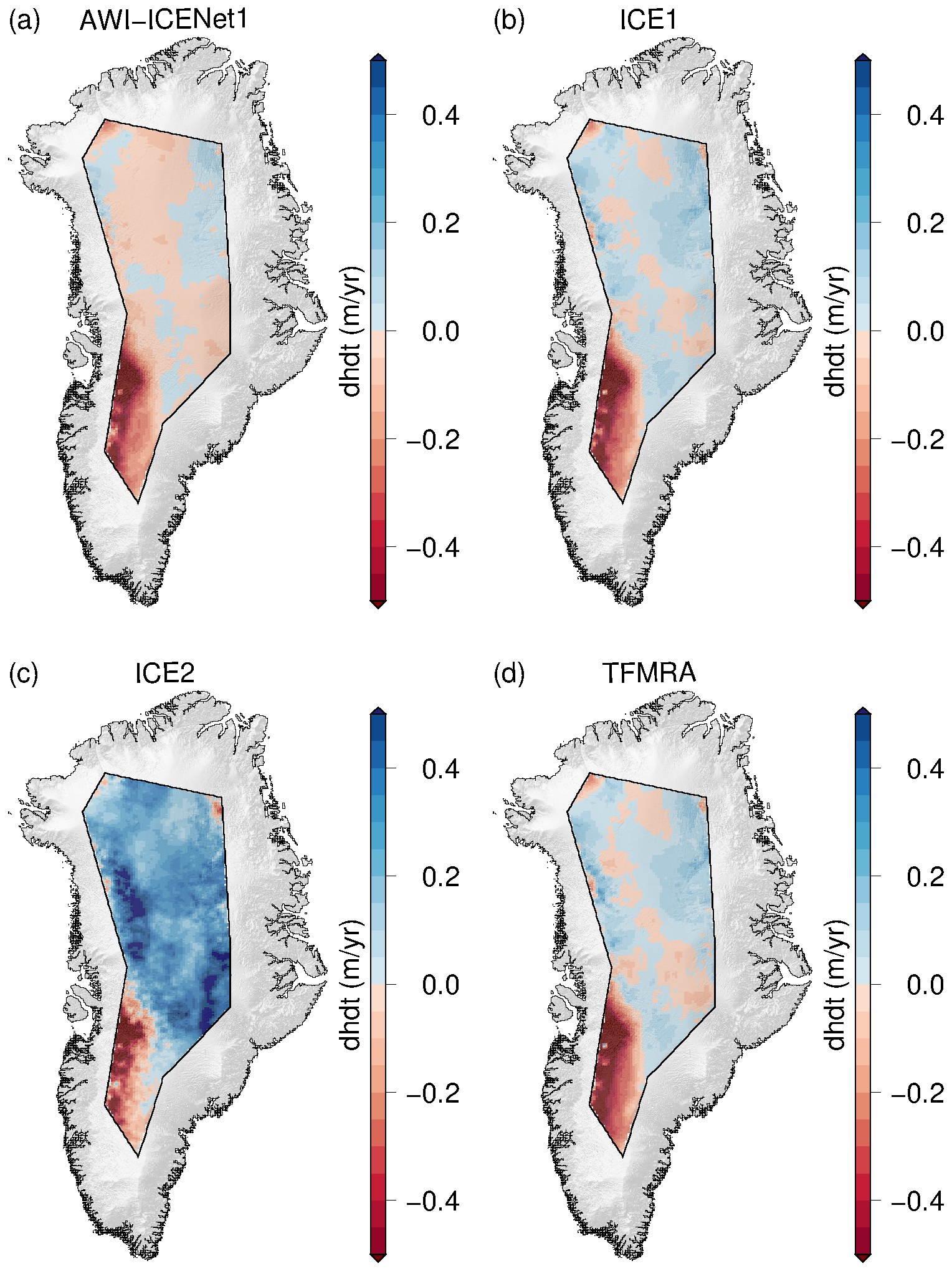
Figure A17Greenland-wide estimates, including corrections for LEW and backscatter, for four retrackers for the period from January 2011 to December 2014, which includes the July melt event of 2012.
The complete simulated reference data set, elevation change grids, and monthly elevation anomalies were uploaded to the World Data Center PANGAEA and can be found in Helm (2024) at https://doi.org/10.1594/PANGAEA.964596.
VH led the study, simulated the waveforms, applied AWI-ICENet1 to satellite data, analysed the results, and contributed figures. AD and EL developed the ConvNet. AD analysed the results and contributed figures. VH and AH wrote large portions of the text. RH wrote machine-learning-specific sections of the text. MH and VH acquired funding for this research. All authors discussed the results and contributed to editing the paper.
The contact author has declared that none of the authors has any competing interests.
Publisher's note: Copernicus Publications remains neutral with regard to jurisdictional claims made in the text, published maps, institutional affiliations, or any other geographical representation in this paper. While Copernicus Publications makes every effort to include appropriate place names, the final responsibility lies with the authors.
The network was trained using a NVIDIA A100 SXM4 80 GB GPU video card and the TensorFlow (version 2.15.0) and Keras (version 2.15.0) packages (Abadi et al., 2015). Waveform retracking was applied on AMD Rome EPYC 7702 cores using the TensorFlow (version 2.15.0) and Keras (version 2.15.0) packages. This work acknowledges PGC Services (including data access). The REMA DEM was provided by the Byrd Polar and Climate Research Center and the Polar Geospatial Center under NSF/OPP awards 1043681, 1542736, 1543501, 1559691, 1810976, and 2129685. The ArcticDEM was provided by the Polar Geospatial Center under NSF/OPP awards 1043681, 1559691, 1542736, 1810976, and 2129685. Access to the ArcticDEM was provided by the Polar Geospatial Center under NSF/OPP awards 1043681, 1559691, and 2129685.
This work was supported by (1) the Deutsche Forschungsgemeinschaft (DFG) as part of Priority Programme 1158 “Antarctic Research with Comparative Investigations in Arctic Ice Areas” (grant no. 442929109), (2) the project “DeepSAR: Physical parameter estimation from SAR data via joint model inversion and deep learning” (grant no. ZT-I-PF-5-9; Helmholtz AI Cooperation Unit), and (3) the Helmholtz Association of German Research Centres as part of the Helmholtz Information and Data Science Incubator and the project “Artificial Intelligence for Cold Regions” (AI-CORE; grant no. ZT-I-0016).
The article processing charges for this open-access publication were covered by the Alfred-Wegener-Institut, Helmholtz-Zentrum für Polar- und Meeresforschung.
This paper was edited by Stef Lhermitte and reviewed by two anonymous referees.
Abadi, M., Agarwal, A., Barham, P., Brevdo, E., Chen, Z., Citro, C., Corrado, G. S., Davis, A., Dean, J., Devin, M., Ghemawat, S., Goodfellow, I., Harp, A., Irving, G., Isard, M., Jia, Y., Jozefowicz, R., Kaiser, L., Kudlur, M., Levenberg, J., Mané, D., Monga, R., Moore, S., Murray, D., Olah, C., Schuster, M., Shlens, J., Steiner, B., Sutskever, I., Talwar, K., Tucker, P., Vanhoucke, V., Vasudevan, V., Viégas, F., Vinyals, O., Warden, P., Wattenberg, M., Wicke, M., Yu, Y., and Zheng, X.: TensorFlow: Large-Scale Machine Learning on Heterogeneous Systems, https://www.tensorflow.org/ (last access: 1 June 2024), 2015. a
Adams, R. and Brown, G.: A model for altimeter returns from penetrable geophysical media, IEEE T. Geosci. Remote, 36, 1784–1793, https://doi.org/10.1109/36.718645, 1998. a
Adodo, F. I., Remy, F., and Picard, G.: Seasonal variations of the backscattering coefficient measured by radar altimeters over the Antarctic Ice Sheet, The Cryosphere, 12, 1767–1778, https://doi.org/10.5194/tc-12-1767-2018, 2018. a
Amarouche, L., Thibaut, P., Zanife, O. Z., Dumont, J.-P., Vincent, P., and Steunou, N.: Improving the Jason-1 Ground Retracking to Better Account for Attitude Effects, Marine Geodesy, 27, 171–197, https://doi.org/10.1080/01490410490465210, 2004. a
Armitage, T. W. K., Wingham, D. J., and Ridout, A. L.: Meteorological Origin of the Static Crossover Pattern Present in Low-Resolution-Mode CryoSat-2 Data Over Central Antarctica, IEEE Geosci. Remote Sens. Lett., 11, 1295–1299, https://doi.org/10.1109/LGRS.2013.2292821, 2014. a, b
Arthern, R. J., Wingham, D. J., and Ridout, A. L.: Controls on ERS altimeter measurements over ice sheets: Footprint-scale topography, backscatter fluctuations, and the dependence of microwave penetration depth on satellite orientation, J. Geophys. Res.-Atmos., 106, 33471–33484, https://doi.org/10.1029/2001JD000498, 2001. a, b
Baumhoer, C. A., Dietz, A. J., Kneisel, C., and Kuenzer, C.: Automated Extraction of Antarctic Glacier and Ice Shelf Fronts from Sentinel-1 Imagery Using Deep Learning, Remote Sens., 11, 2529, https://doi.org/10.3390/rs11212529, 2019. a
Brown, G.: The average impulse response of a rough surface and its applications, IEEE T. Antenn. Propag., 25, 67–74, https://doi.org/10.1109/TAP.1977.1141536, 1977. a, b
Buzzanga, B., Heijkoop, E., Hamlington, B. D., Nerem, R. S., and Gardner, A.: An Assessment of Regional ICESat-2 Sea-Level Trends, Geophys. Res. Lett., 48, e2020GL092327, https://doi.org/10.1029/2020GL092327, 2021. a
Cai, Y., Hu, S., Lang, S., Guo, Y., and Liu, J.: End-to-End Classification Network for Ice Sheet Subsurface Targets in Radar Imagery, Appl. Sci., 10, 2501, https://doi.org/10.3390/app10072501, 2020. a
Campos-Taberner, M., Garcia-Haro, F. J., Martinez, B., Izquierdo-Verdiguier, E., Atzberger, C., Camps-Valls, G., and Gilabert, M. A.: Understanding deep learning in land use classification based on Sentinel-2 time series, Sci. Rep.-UK, 10, 17188, https://doi.org/10.1038/s41598-020-74215-5, 2020. a
Christie, F. D. W., Steig, E. J., Gourmelen, N., Tett, S. F. B., and Bingham, R. G.: Inter-decadal climate variability induces differential ice response along Pacific-facing West Antarctica, Nat. Commun., 14, 93, https://doi.org/10.1038/s41467-022-35471-3, 2023. a
Dalsasso, E., Denis, L., and Tupin, F.: As If by Magic: Self-Supervised Training of Deep Despeckling Networks With MERLIN, IEEE T. Geosci. Remote, 60, 1–13, https://doi.org/10.1109/TGRS.2021.3128621, 2022. a
Davis, C.: A robust threshold retracking algorithm for measuring ice-sheet surface elevation change from satellite radar altimeters, IEEE T. Geosci. Remote, 35, 974–979, https://doi.org/10.1109/36.602540, 1997. a, b, c
Davis, C. H. and Zwally, H. J.: Geographic and seasonal variations in the surface properties of the ice sheets by satellite-radar altimetry, J. Glaciol., 39, 687–697, https://doi.org/10.3189/S0022143000016580, 1993. a
Davison, B. J., Hogg, A. E., Rigby, R., Veldhuijsen, S., van Wessem, J. M., van den Broeke, M. R., Holland, P. R., Selley, H. L., and Dutrieux, P.: Sea level rise from West Antarctic mass loss significantly modified by large snowfall anomalies, Nat. Commun., 14, 1479, https://doi.org/10.1038/s41467-023-36990-3, 2023. a
Dinardo, S., Fenoglio-Marc, L., Buchhaupt, C., Becker, M., Scharroo, R., Joana Fernandes, M., and Benveniste, J.: Coastal SAR and PLRM altimetry in German Bight and West Baltic Sea, Adv. Space Res., 62, 1371–1404, https://doi.org/10.1016/j.asr.2017.12.018, 2018. a
Dinardo, S., Fenoglio-Marc, L., Becker, M., Scharroo, R., Fernandes, M. J., Staneva, J., Grayek, S., and Benveniste, J.: A RIP-based SAR retracker and its application in North East Atlantic with Sentinel-3, Adv. Space Res., 68, 892–929, https://doi.org/10.1016/j.asr.2020.06.004, 2021. a
Dong, S., Tang, X., Guo, J., Fu, L., Chen, X., and Sun, B.: EisNet: Extracting Bedrock and Internal Layers From Radiostratigraphy of Ice Sheets With Machine Learning, IEEE T. Geosci. Remote, 60, 1–12, https://doi.org/10.1109/TGRS.2021.3136648, 2022. a
Donini, E., Bovolo, F., and Bruzzone, L.: A Deep Learning Architecture for Semantic Segmentation of Radar Sounder Data, IEEE T. Geosci. Remote, 60, 1–14, https://doi.org/10.1109/TGRS.2021.3125773, 2022. a
Dubayah, R., Blair, J. B., Goetz, S., Fatoyinbo, L., Hansen, M., Healey, S., Hofton, M., Hurtt, G., Kellner, J., Luthcke, S., Armston, J., Tang, H., Duncanson, L., Hancock, S., Jantz, P., Marselis, S., Patterson, P. L., Qi, W., and Silva, C.: The Global Ecosystem Dynamics Investigation: High-resolution laser ranging of the Earth's forests and topography, Sci. Remote Sens., 1, 100002, https://doi.org/10.1016/j.srs.2020.100002, 2020. a
Exprivia: Baseline E Evolutions, https://earth.esa.int/eogateway/documents/20142/37627/Cryosat-Baseline-E-Evolutions.pdf (last access: 1 June 2024), 2021. a, b
Fayad, I., Ienco, D., Baghdadi, N., Gaetano, R., Alvares, C. A., Stape, J. L., Ferraço Scolforo, H., and Le Maire, G.: A CNN-based approach for the estimation of canopy heights and wood volume from GEDI waveforms, Remote Sens. Environ., 265, 112652, https://doi.org/10.1016/j.rse.2021.112652, 2021. a, b, c, d, e, f, g, h
Femenias, P., Remy, F., Raizonville, R., and Minster, J. F.: Analysis of satellite-altimeter height measurements above continental ice sheets, J. Glaciol., 39, 591–600, https://doi.org/10.3189/S0022143000016488, 1993. a, b, c, d, e
Flament, T. and Rémy, F.: Dynamic thinning of Antarctic glaciers from along-track repeat radar altimetry, J. Glaciol., 58, 830–840, https://doi.org/10.3189/2012JoG11J118, 2012. a, b, c
Frappart, F., Legrésy, B., Niño, F., Blarel, F., Fuller, N., Fleury, S., Birol, F., and Calmant, S.: An ERS-2 altimetry reprocessing compatible with ENVISAT for long-term land and ice sheets studies, Remote Sens. Environ., 184, 558–581, https://doi.org/10.1016/j.rse.2016.07.037, 2016. a
García, M. H., Donini, E., and Bovolo, F.: Automatic Segmentation of Ice Shelves with Deep Learning, in: 2021 IEEE International Geoscience and Remote Sensing Symposium IGARSS, 4833–4836, https://doi.org/10.1109/IGARSS47720.2021.9553610, 2021. a
Ghosh, R. and Bovolo, F.: TransSounder: A Hybrid TransUNet-TransFuse Architectural Framework for Semantic Segmentation of Radar Sounder Data, IEEE T. Geosci. Remote, 60, 1–13, https://doi.org/10.1109/TGRS.2022.3180761, 2022. a
Hanna, E., Navarro, F. J., Pattyn, F., Domingues, C. M., Fettweis, X., Ivins, E. R., Nicholls, R. J., Ritz, C., Smith, B., Tulaczyk, S., Whitehouse, P. L., and Zwally, H. J.: Ice-sheet mass balance and climate change, Nature, 498, 51–59, https://doi.org/10.1038/nature12238, 2013. a
He, K., Zhang, X., Ren, S., and Sun, J.: Deep Residual Learning for Image Recognition, in: 2016 IEEE Conference on Computer Vision and Pattern Recognition (CVPR), 770–778, https://doi.org/10.1109/CVPR.2016.90, 2016. a
Helm, V.: Convolutional neural network training dataset and results of AWI-ICENet1 retracker, PANGAEA [data set], https://doi.org/10.1594/PANGAEA.964596, 2024. a
Helm, V., Humbert, A., and Miller, H.: Elevation and elevation change of Greenland and Antarctica derived from CryoSat-2, The Cryosphere, 8, 1539–1559, https://doi.org/10.5194/tc-8-1539-2014, 2014. a, b, c, d, e, f, g
Howat, I., Porter, C., Noh, M.-J., Husby, E., Khuvis, S., Danish, E., Tomko, K., Gardiner, J., Negrete, A., Yadav, B., Klassen, J., Kelleher, C., Cloutier, M., Bakker, J., Enos, J., Arnold, G., Bauer, G., and Morin, P.: The Reference Elevation Model of Antarctica – Mosaics, Version 2, Harvard Dataverse [data set], https://doi.org/10.7910/DVN/EBW8UC, 2022. a
Howat, I. M., Porter, C., Smith, B. E., Noh, M.-J., and Morin, P.: The Reference Elevation Model of Antarctica, The Cryosphere, 13, 665–674, https://doi.org/10.5194/tc-13-665-2019, 2019. a
Joughin, I. and Alley, R. B.: Stability of the West Antarctic ice sheet in a warming world, Nat. Geosci., 4, 506–513, https://doi.org/10.1038/ngeo1194, 2011. a
Kamangir, H., Rahnemoonfar, M., Dobbs, D., Paden, J., and Fox, G.: Deep Hybrid Wavelet Network for Ice Boundary Detection in Radra Imagery, in: IGARSS 2018 – 2018 IEEE International Geoscience and Remote Sensing Symposium, 3449–3452, https://doi.org/10.1109/IGARSS.2018.8518617, 2018. a
Kingma, D. P. and Ba, J.: Adam: A Method for Stochastic Optimization, ArXiv [preprint], https://doi.org/10.48550/ARXIV.1412.6980, 2014. a
Krizhevsky, A., Sutskever, I., and Hinton, G. E.: ImageNet Classification with Deep Convolutional Neural Networks, in: Advances in Neural Information Processing Systems, edited by Pereira, F., Burges, C., Bottou, L., and Weinberger, K., vol. 25, Curran Associates, Inc., https://proceedings.neurips.cc/paper_files/paper/2012/file/c399862d3b9d6b76c8436e924a68c45b-Paper.pdf (last access: 1 June 2024), 2012. a
Lacroix, P., Dechambre, M., Legrésy, B., Blarel, F., and Rémy, F.: On the use of the dual-frequency ENVISAT altimeter to determine snowpack properties of the Antarctic ice sheet, Remote Sens. Environ., 112, 1712–1729, https://doi.org/10.1016/j.rse.2007.08.022, 2008. a, b
Lang, N., Jetz, W., Schindler, K., and Wegner, J. D.: A high-resolution canopy height model of the Earth, arXiv [preprint], arXiv:2204.08322, 2022. a
Larour, E., Ivins, E. R., and Adhikari, S.: Should coastal planners have concern over where land ice is melting?, Sci. Adv., 3, e1700537, https://doi.org/10.1126/sciadv.1700537, 2017. a
Larue, F., Picard, G., Aublanc, J., Arnaud, L., Robledano-Perez, A., LE Meur, E., Favier, V., Jourdain, B., Savarino, J., and Thibaut, P.: Radar altimeter waveform simulations in Antarctica with the Snow Microwave Radiative Transfer Model (SMRT), Remote Sens. Environ., 263, 112534, https://doi.org/10.1016/j.rse.2021.112534, 2021. a
LeCun, Y., Bengio, Y., and Hinton, G.: Deep learning, Nature, 521, 436–444, https://doi.org/10.1038/nature14539, 2015. a
Lee, S., Im, J., Kim, J., Kim, M., Shin, M., Kim, H.-C., and Quackenbush, L. J.: Arctic Sea Ice Thickness Estimation from CryoSat-2 Satellite Data Using Machine Learning-Based Lead Detection, Remote Sens., 8, 698, https://doi.org/10.3390/rs8090698, 2016. a
Legresy, B., Remy, F., and Schaeffer, P.: Different ERS altimeter measurements between ascending and descending tracks caused by wind induced features over ice sheets, Geophys. Res. Lett., 26, 2231–2234, https://doi.org/10.1029/1999GL900531, 1999. a
Legresy, B., Papa, F., Remy, F., Vinay, G., van den Bosch, M., and Zanife, O.-Z.: ENVISAT radar altimeter measurements over continental surfaces and ice caps using the ICE-2 retracking algorithm, Remote Sens. Environ., 95, 150–163, https://doi.org/10.1016/j.rse.2004.11.018, 2005. a, b
Legrésy, B. and Rémy, F.: Altimetric observations of surface characteristics of the Antarctic ice sheet, J. Glaciol., 43, 265–275, https://doi.org/10.3189/S002214300000321X, 1997. a, b, c
Li, W., Slobbe, C., and Lhermitte, S.: A leading-edge-based method for correction of slope-induced errors in ice-sheet heights derived from radar altimetry, The Cryosphere, 16, 2225–2243, https://doi.org/10.5194/tc-16-2225-2022, 2022. a
Liu-Schiaffini, M., Ng, G., Grima, C., and Young, D.: Ice Thickness From Deep Learning and Conditional Random Fields: Application to Ice-Penetrating Radar Data With Radiometric Validation, IEEE T. Geosci. Remote, 60, 1–14, https://doi.org/10.1109/TGRS.2022.3214147, 2022. a
Loebel, E., Scheinert, M., Horwath, M., Heidler, K., Christmann, J., Phan, L. D., Humbert, A., and Zhu, X. X.: Extracting Glacier Calving Fronts by Deep Learning: The Benefit of Multispectral, Topographic, and Textural Input Features, IEEE T. Geosci. Remote, 60, 1–12, https://doi.org/10.1109/TGRS.2022.3208454, 2022. a
Loebel, E., Scheinert, M., Horwath, M., Humbert, A., Sohn, J., Heidler, K., Liebezeit, C., and Zhu, X. X.: Calving front monitoring at sub-seasonal resolution: a deep learning application to Greenland glaciers, The Cryosphere Discuss. [preprint], https://doi.org/10.5194/tc-2023-52, in review, 2023. a
Markus, T., Neumann, T., Martino, A., Abdalati, W., Brunt, K., Csatho, B., Farrell, S., Fricker, H., Gardner, A., Harding, D., Jasinski, M., Kwok, R., Magruder, L., Lubin, D., Luthcke, S., Morison, J., Nelson, R., Neuenschwander, A., Palm, S., Popescu, S., Shum, C., Schutz, B. E., Smith, B., Yang, Y., and Zwally, J.: The Ice, Cloud, and land Elevation Satellite-2 (ICESat-2): Science requirements, concept, and implementation, Remote Sens. Environ., 190, 260–273, https://doi.org/10.1016/j.rse.2016.12.029, 2017. a
Martin, T. V., Zwally, H. J., Brenner, A. C., and Bindschadler, R. A.: Analysis and retracking of continental ice sheet radar altimeter waveforms, J. Geophys. Res.-Oceans, 88, 1608–1616, https://doi.org/10.1029/JC088iC03p01608, 1983. a
McMillan, M., Leeson, A., Shepherd, A., Briggs, K., Armitage, T. W. K., Hogg, A., Kuipers Munneke, P., van den Broeke, M., Noël, B., van de Berg, W. J., Ligtenberg, S., Horwath, M., Groh, A., Muir, A., and Gilbert, L.: A high-resolution record of Greenland mass balance, Geophys. Res. Lett., 43, 7002–7010, https://doi.org/10.1002/2016GL069666, 2016. a, b, c, d
Michel, A., Flament, T., and Rémy, F.: Study of the Penetration Bias of ENVISAT Altimeter Observations over Antarctica in Comparison to ICESat Observations, Remote Sens., 6, 9412–9434, https://doi.org/10.3390/rs6109412, 2014. a
Milillo, P., Rignot, E., Rizzoli, P., Scheuchl, B., Mouginot, J., Bueso-Bello, J. L., Prats-Iraola, P., and Dini, L.: Rapid glacier retreat rates observed in West Antarctica, Nat. Geosci., 15, 48–53, https://doi.org/10.1038/s41561-021-00877-z, 2022. a
Mohajerani, Y., Jeong, S., Scheuchl, B., Velicogna, I., Rignot, E., and Milillo, P.: Automatic delineation of glacier grounding lines in differential interferometric synthetic-aperture radar data using deep learning, Sci. Rep.-UK, 11, 4992, https://doi.org/10.1038/s41598-021-84309-3, 2021. a
Mouginot, J., Rignot, E., and Scheuchl, B.: Sustained increase in ice discharge from the Amundsen Sea Embayment, West Antarctica, from 1973 to 2013, Geophys. Res. Lett., 41, 1576–1584, https://doi.org/10.1002/2013GL059069, 2014. a
Müller, F. L., Dettmering, D., Bosch, W., and Seitz, F.: Monitoring the Arctic Seas: How Satellite Altimetry Can Be Used to Detect Open Water in Sea-Ice Regions, Remote Sens., 9, 551, https://doi.org/10.3390/rs9060551, 2017. a
Nield, G. A., Whitehouse, P. L., King, M. A., and Clarke, P. J.: Glacial isostatic adjustment in response to changing Late Holocene behaviour of ice streams on the Siple Coast, West Antarctica, Geophys. J. Int., 205, 1–21, https://doi.org/10.1093/gji/ggv532, 2016. a
Nilsson, J., Vallelonga, P., Simonsen, S. B., Sørensen, L. S., Forsberg, R., Dahl-Jensen, D., Hirabayashi, M., Goto-Azuma, K., Hvidberg, C. S., Kjær, H. A., and Satow, K.: Greenland 2012 melt event effects on CryoSat-2 radar altimetry, Geophys. Res. Lett., 42, 3919–3926, https://doi.org/10.1002/2015GL063296, 2015. a, b, c
Nilsson, J., Gardner, A., Sandberg Sørensen, L., and Forsberg, R.: Improved retrieval of land ice topography from CryoSat-2 data and its impact for volume-change estimation of the Greenland Ice Sheet, The Cryosphere, 10, 2953–2969, https://doi.org/10.5194/tc-10-2953-2016, 2016. a, b
Nilsson, J., Gardner, A. S., and Paolo, F. S.: Elevation change of the Antarctic Ice Sheet: 1985 to 2020, Earth Syst. Sci. Data, 14, 3573–3598, https://doi.org/10.5194/essd-14-3573-2022, 2022. a, b, c, d, e
NSIDC: Guide for Applying ICESat Inter-campaign Bias Corrections (ICBs), https://nsidc.org/sites/default/files/icesat-intercampaign-bias-corrections.pdf (last access: 1 June 2024), 2021. a
Otosaka, I. N., Shepherd, A., Ivins, E. R., Schlegel, N.-J., Amory, C., van den Broeke, M. R., Horwath, M., Joughin, I., King, M. D., Krinner, G., Nowicki, S., Payne, A. J., Rignot, E., Scambos, T., Simon, K. M., Smith, B. E., Sørensen, L. S., Velicogna, I., Whitehouse, P. L., A, G., Agosta, C., Ahlstrøm, A. P., Blazquez, A., Colgan, W., Engdahl, M. E., Fettweis, X., Forsberg, R., Gallée, H., Gardner, A., Gilbert, L., Gourmelen, N., Groh, A., Gunter, B. C., Harig, C., Helm, V., Khan, S. A., Kittel, C., Konrad, H., Langen, P. L., Lecavalier, B. S., Liang, C.-C., Loomis, B. D., McMillan, M., Melini, D., Mernild, S. H., Mottram, R., Mouginot, J., Nilsson, J., Noël, B., Pattle, M. E., Peltier, W. R., Pie, N., Roca, M., Sasgen, I., Save, H. V., Seo, K.-W., Scheuchl, B., Schrama, E. J. O., Schröder, L., Simonsen, S. B., Slater, T., Spada, G., Sutterley, T. C., Vishwakarma, B. D., van Wessem, J. M., Wiese, D., van der Wal, W., and Wouters, B.: Mass balance of the Greenland and Antarctic ice sheets from 1992 to 2020, Earth Syst. Sci. Data, 15, 1597–1616, https://doi.org/10.5194/essd-15-1597-2023, 2023. a
Porter, C., Howat, I., Noh, M.-J., Husby, E., Khuvis, S., Danish, E., Tomko, K., Gardiner, J., Negrete, A., Yadav, B., Klassen, J., Kelleher, C., Cloutier, M., Bakker, J., Enos, J., Arnold, G., Bauer, G., and Morin, P.: ArcticDEM – Mosaics, Version 4.1, Harvard Dataverse [data set], https://doi.org/10.7910/DVN/3VDC4W, 2023. a
Richter, A., Popov, S. V., Fritsche, M., Lukin, V. V., Matveev, A. Y., Ekaykin, A. A., Lipenkov, V. Y., Fedorov, D. V., Eberlein, L., Schröder, L., Ewert, H., Horwath, M., and Dietrich, R.: Height changes over subglacial Lake Vostok, East Antarctica: Insights from GNSS observations, J. Geophys. Res.-Earth Surf., 119, 2460–2480, https://doi.org/10.1002/2014JF003228, 2014. a, b
Ridley, J. K. and Partington, K. C.: A model of satellite radar altimeter return from ice sheets, Int. J. Remote Sens., 9, 601–624, https://doi.org/10.1080/01431168808954881, 1988. a, b
Rignot, E., Vaughan, D. G., Schmeltz, M., Dupont, T., and Macayeal, D.: Acceleration of Pine Island and Thwaites Glaciers, West Antarctica, Ann. Glaciol., 34, 189–194, https://doi.org/10.3189/172756402781817950, 2002. a
Rignot, E., Mouginot, J., Morlighem, M., Seroussi, H., and Scheuchl, B.: Widespread, rapid grounding line retreat of Pine Island, Thwaites, Smith, and Kohler glaciers, West Antarctica, from 1992 to 2011, Geophys. Res. Lett., 41, 3502–3509, https://doi.org/10.1002/2014GL060140, 2014. a
Roemer, S., Legrésy, B., Horwath, M., and Dietrich, R.: Refined analysis of radar altimetry data applied to the region of the subglacial Lake Vostok/Antarctica, Remote Sens. Environ., 106, 269–284, https://doi.org/10.1016/j.rse.2006.02.026, 2007. a, b, c
Ronneberger, O., Fischer, P., and Brox, T.: U-Net: Convolutional Networks for Biomedical Image Segmentation, ArXiv [preprint], abs/1505.04597, https://api.semanticscholar.org/CorpusID:3719281 (last access: 1 June 2024), 2015. a
Scambos, T., Bell, R., Alley, R., Anandakrishnan, S., Bromwich, D., Brunt, K., Christianson, K., Creyts, T., Das, S., DeConto, R., Dutrieux, P., Fricker, H., Holland, D., MacGregor, J., Medley, B., Nicolas, J., Pollard, D., Siegfried, M., Smith, A., Steig, E., Trusel, L., Vaughan, D., and Yager, P.: How much, how fast?: A science review and outlook for research on the instability of Antarctica's Thwaites Glacier in the 21st century, Global Planet. Change, 153, 16–34, https://doi.org/10.1016/j.gloplacha.2017.04.008, 2017. a
Scheuchl, B., Mouginot, J., Rignot, E., Morlighem, M., and Khazendar, A.: Grounding line retreat of Pope, Smith, and Kohler Glaciers, West Antarctica, measured with Sentinel-1a radar interferometry data, Geophys. Res. Lett., 43, 8572–8579, https://doi.org/10.1002/2016GL069287, 2016. a
Schröder, L., Horwath, M., Dietrich, R., Helm, V., van den Broeke, M. R., and Ligtenberg, S. R. M.: Four decades of Antarctic surface elevation changes from multi-mission satellite altimetry, The Cryosphere, 13, 427–449, https://doi.org/10.5194/tc-13-427-2019, 2019. a, b, c, d, e
Shen, X., Zhang, J., Zhang, X., Meng, J., and Ke, C.: Sea Ice Classification Using Cryosat-2 Altimeter Data by Optimal Classifier–Feature Assembly, IEEE Geosci. Remote Sens. Lett., 14, 1948–1952, https://doi.org/10.1109/LGRS.2017.2743339, 2017a. a
Shen, X.-y., Zhang, J., Meng, J.-m., Zhang, J., and Ke, C.-q.: Sea ice type classification based on random forest machine learning with Cryosat-2 altimeter data, in: 2017 International Workshop on Remote Sensing with Intelligent Processing (RSIP), 1–5, https://doi.org/10.1109/RSIP.2017.7958792, 2017b. a
Shepherd, A., Ivins, E., Rignot, E., Smith, B., van den Broeke, M., Velicogna, I., Whitehouse, P., Briggs, K., Joughin, I., Krinner, G., Nowicki, S., Payne, T., Scambos, T., Schlegel, N., A, G., Agosta, C., Ahlstrøm, A., Babonis, G., Barletta, V., Blazquez, A., Bonin, J., Csatho, B., Cullather, R., Felikson, D., Fettweis, X., Forsberg, R., Gallee, H., Gardner, A., Gilbert, L., Groh, A., Gunter, B., Hanna, E., Harig, C., Helm, V., Horvath, A., Horwath, M., Khan, S., Kjeldsen, K. K., Konrad, H., Langen, P., Lecavalier, B., Loomis, B., Luthcke, S., McMillan, M., Melini, D., Mernild, S., Mohajerani, Y., Moore, P., Mouginot, J., Moyano, G., Muir, A., Nagler, T., Nield, G., Nilsson, J., Noel, B., Otosaka, I., Pattle, M. E., Peltier, W. R., Pie, N., Rietbroek, R., Rott, H., Sandberg-Sørensen, L., Sasgen, I., Save, H., Scheuchl, B., Schrama, E., Schröder, L., Seo, K.-W., Simonsen, S., Slater, T., Spada, G., Sutterley, T., Talpe, M., Tarasov, L., van de Berg, W. J., van der Wal, W., van Wessem, M., Vishwakarma, B. D., Wiese, D., Wouters, B., and Team, T. I.: Mass balance of the Antarctic Ice Sheet from 1992 to 2017, Nature, 558, 219–222, https://doi.org/10.1038/s41586-018-0179-y, 2018. a
Simonsen, S. B. and Sørensen, L. S.: Implications of changing scattering properties on Greenland ice sheet volume change from Cryosat-2 altimetry, Remote Sens. Environ., 190, 207–216, https://doi.org/10.1016/j.rse.2016.12.012, 2017. a, b, c, d, e, f, g, h, i
Slater, T., Shepherd, A., Mcmillan, M., Armitage, T. W. K., Otosaka, I., and Arthern, R. J.: Compensating Changes in the Penetration Depth of Pulse-Limited Radar Altimetry Over the Greenland Ice Sheet, IEEE T. Geosci. Remote, 57, 9633–9642, https://doi.org/10.1109/TGRS.2019.2928232, 2019. a
Smith, B., Fricker, H. A., Gardner, A. S., Medley, B., Nilsson, J., Paolo, F. S., Holschuh, N., Adusumilli, S., Brunt, K., Csatho, B., Harbeck, K., Markus, T., Neumann, T., Siegfried, M. R., and Zwally, H. J.: Pervasive ice sheet mass loss reflects competing ocean and atmosphere processes, Science, 368, 1239–1242, https://doi.org/10.1126/science.aaz5845, 2020. a, b, c
Smith, B., Adusumilli, S., Csathó, B. M., Felikson, D., Fricker, H. A., Gardner, A., Holschuh, N., Lee, J., Nilsson, J., Paolo, F. S., Siegfried, M. R., Sutterley, T., and the ICESat-2 Science Team: ATLAS/ICESat-2 L3A Land Ice Height, Version 6, Boulder, Colorado USA, NASA National Snow and Ice Data Center Distributed Active Archive Center[data set], https://doi.org/10.5067/ATLAS/ATL06.006, 2023. a
Studinger, M., Smith, B. E., Kurtz, N., Petty, A., Sutterley, T., and Tilling, R.: Estimating differential penetration of green (532 nm) laser light over sea ice with NASA's Airborne Topographic Mapper: observations and models, The Cryosphere, 18, 2625–2652, https://doi.org/10.5194/tc-18-2625-2024, 2024. a, b
Thibaut, P., Poisson, J. C., Bronner, E., and Picot, N.: Relative Performance of the MLE3 and MLE4 Retracking Algorithms on Jason-2 Altimeter Waveforms, Marine Geodesy, 33, 317–335, https://doi.org/10.1080/01490419.2010.491033, 2010. a
Thibaut, P., Piras, F., Roinard, H., Guerou, A., Boy, F., Maraldi, C., Bignalet-Cazalet, F., Dibarboure, G., and Picot, N.: Benefits of the “Adaptive Retracking Solution” for the JASON-3 GDR-F Reprocessing Campaign, in: 2021 IEEE International Geoscience and Remote Sensing Symposium IGARSS, 7422–7425, https://doi.org/10.1109/IGARSS47720.2021.9553647, 2021. a
Wingham, D., Rapley, C., and Griffiths, H.: New Techniques in Satellite Altimeter Tracking Systems, Digest – International Geoscience and Remote Sensing Symposium (IGARSS), 8–11 September 1986, Zurich, Switzerland, 1986. a, b
Wingham, D., Francis, C., Baker, S., Bouzinac, C., Brockley, D., Cullen, R., de Chateau-Thierry, P., Laxon, S., Mallow, U., Mavrocordatos, C., Phalippou, L., Ratier, G., Rey, L., Rostan, F., Viau, P., and Wallis, D.: CryoSat: A mission to determine the fluctuations in Earth’s land and marine ice fields, Adv. Space Res., 37, 841–871, https://doi.org/10.1016/j.asr.2005.07.027, 2006. a
Xia, X. and Kulis, B.: W-Net: A Deep Model for Fully Unsupervised Image Segmentation, arXiv [preprint], 1711.08506, https://doi.org/10.48550/arXiv.1711.08506, 2017. a
Zwally, H. J., Schutz, R., Bentley, C., Bufton, J., Herring, T., Minster, J., Spinhirne, J., and Thomas, R.: GLAS/ICESat L2 Antarctic and Greenland Ice Sheet Altimetry Data, Version 34, Boulder, Colorado USA, NASA National Snow and Ice Data Center Distributed Active Archive Center [data set], https://doi.org/10.5067/ICESAT/GLAS/DATA225, 2014. a