the Creative Commons Attribution 4.0 License.
the Creative Commons Attribution 4.0 License.
 | 20 Aug 2024
Toward long-term monitoring of regional permafrost thaw with satellite interferometric synthetic aperture radar
Franz J. Meyer
Timothy H. Dixon
Active-layer thickness (ALT) is estimated for a study area in northern Alaska's continuous-permafrost zone using satellite data from Sentinel-1 (radar) and ICESat-2 (lidar) for the period 2017 to 2022. Synthetic aperture radar (SAR) interferograms were generated using the Short Baseline Subset (SBAS) approach. Displacement time series over the thaw season (June–September) are fit well with a linear model (root mean square error (RMSE) scatter is less than 7 mm) and show maximum seasonal subsidence of 20–60 mm. ICESat-2 products were used to validate the interferometric synthetic aperture radar (InSAR) displacement time series. ALT was estimated from measured subsidence using a widely used model exploiting the volume difference between ice and water, reaching a maximum depth in our study area of 1.5 m. Estimated ALT is in good agreement with in situ and other remotely sensed data but is sensitive to assumed thaw season onset, indicating the need for reliable surface temperature data. Our results suggest the feasibility of long-term permafrost monitoring with satellite InSAR. However, the C-band (∼55 mm center wavelength) Sentinel radar is sensitive to vegetation cover and, in our studies, was not successful for similar monitoring in the heavily treed discontinuous-permafrost zone of central Alaska.
- Article
(9136 KB) - Full-text XML
-
Supplement
(1821 KB) - BibTeX
- EndNote


Permafrost is usually covered with soil or sediment – the active layer – which freezes and thaws seasonally. The annual freeze–thaw cycle causes surface height changes due to the volume difference between ice and liquid water. Active-layer thickness (ALT) can be estimated from the magnitude of surface subsidence during the thaw season using simplified physical models (Liu et al., 2012, 2014, 2015; Schaefer et al., 2015; Hu et al., 2018). ALT is expected to increase as Arctic temperatures rise and as permafrost undergoes long-term thaw, releasing carbon dioxide and methane, both of which are powerful greenhouse gases. The process thus represents a potentially powerful positive feedback in the global climate system (e.g., Schaefer et al., 2009; Turetsky et al., 2020). On the other hand, the active layer can also moderate the impact of surface temperature changes on deeper permafrost (Dobinski, 2011), perhaps limiting rapid increases in ALT. Frequent monitoring of ALT across the Arctic landscape is clearly important, implying the need for remote sensing approaches.
In the last 3 decades, satellite-based interferometric synthetic aperture radar (InSAR) has been used to monitor a variety of Earth processes that generate subtle surface displacements, including earthquake and volcano deformation and reservoir compaction from fluid withdrawal (e.g., Bürgmann et al., 2000). Recent examples include earthquake after-slip (e.g., Sadeghi Chorsi et al., 2022b, a), volcano deformation (e.g., Poland and Zebker, 2022; Grapenthin et al., 2022), groundwater extraction (e.g., Castellazzi et al., 2016), carbon sequestration (e.g., Yang et al., 2015; Vasco et al., 2020), seismicity induced by fluid injection (e.g., Deng et al., 2020), coastal sea ice dynamics (e.g., Dammann et al., 2019), glacier velocity estimation (e.g., Strozzi et al., 2020), and coastal flood hazards (e.g., Bekaert et al., 2017; Zhang et al., 2022). Pioneering work by Liu et al. (2010, 2012) demonstrated the utility of InSAR to monitor long-term permafrost thaw and changes in ALT.
Here, we use InSAR from the Sentinel-1 satellite constellation to investigate permafrost thaw on part of the North Slope of Alaska for the period 2017 to 2022, focusing on multi-year changes in ALT and using available ICESat-2 lidar data to validate the InSAR result. Our study has the following objectives: (1) to examine the spatial distribution of seasonal thaw subsidence amplitude using SAR interferometry from 2017 to 2022, (2) to use the annual variation of InSAR-measured displacements to estimate ALT and to compare this to long-term in situ ALT observations, (3) to assess the ability of the ICESat-2 ATL08 product to complement InSAR data in permafrost regions, and (4) to test the influence of some environmental factors on the yearly variations in ALT.
Satellite remote sensing of permafrost has been ongoing for at least 3 decades (e.g., Peddle and Franklin, 1993), focusing on landslides and wildfires, thermokarst processes, and soil moisture dynamics. The synthetic aperture radar (SAR) data used in many of these studies come from satellites – including Radarsat-1, Envisat, JERS-1, ERS-1 and -2, ALOS PALSAR, TanDEM-X, COSMO-Skymed, TerraSAR-X, Envisat, and Sentinel-1 – and airborne sensors – including UAVSAR and AirMOSS. GNSS has also been exploited using the GPS-IR (GPS interferometric reflectometry) technique. These studies have been conducted in northern and central Alaska, northern and western Canada, Greenland, Antarctica, Russia, and Tibet and have contributed to our understanding of permafrost dynamics, providing insights into seasonal and long-term changes in permafrost regions. Table 1 summarizes these microwave-based studies, categorizing them into three main technical applications: (1) seasonal thaw, (2) seasonal and long-term subsidence, and (3) ALT estimation and other scientific applications. The papers that are most relevant to this study include Liu et al. (2010, 2012, 2015) and Schaefer et al. (2015).
Singhroy et al. (2007)Rykhus and Lu (2008)Liu et al. (2010)Iwahana et al. (2016)Strozzi et al. (2018)Zwieback et al. (2018)Bartsch et al. (2019)Wang et al. (2020)Liu et al. (2012)Daout et al. (2017)Chen et al. (2018)Liu and Larson (2018)Hu et al. (2018)Michaelides et al. (2019)Chen et al. (2020)Bernhard et al. (2020)Honglei et al. (2021)Liu et al. (2012)Schaefer et al. (2015)Michaelides et al. (2019)Chen et al. (2020)Michaelides et al. (2021b)Chen et al. (2023)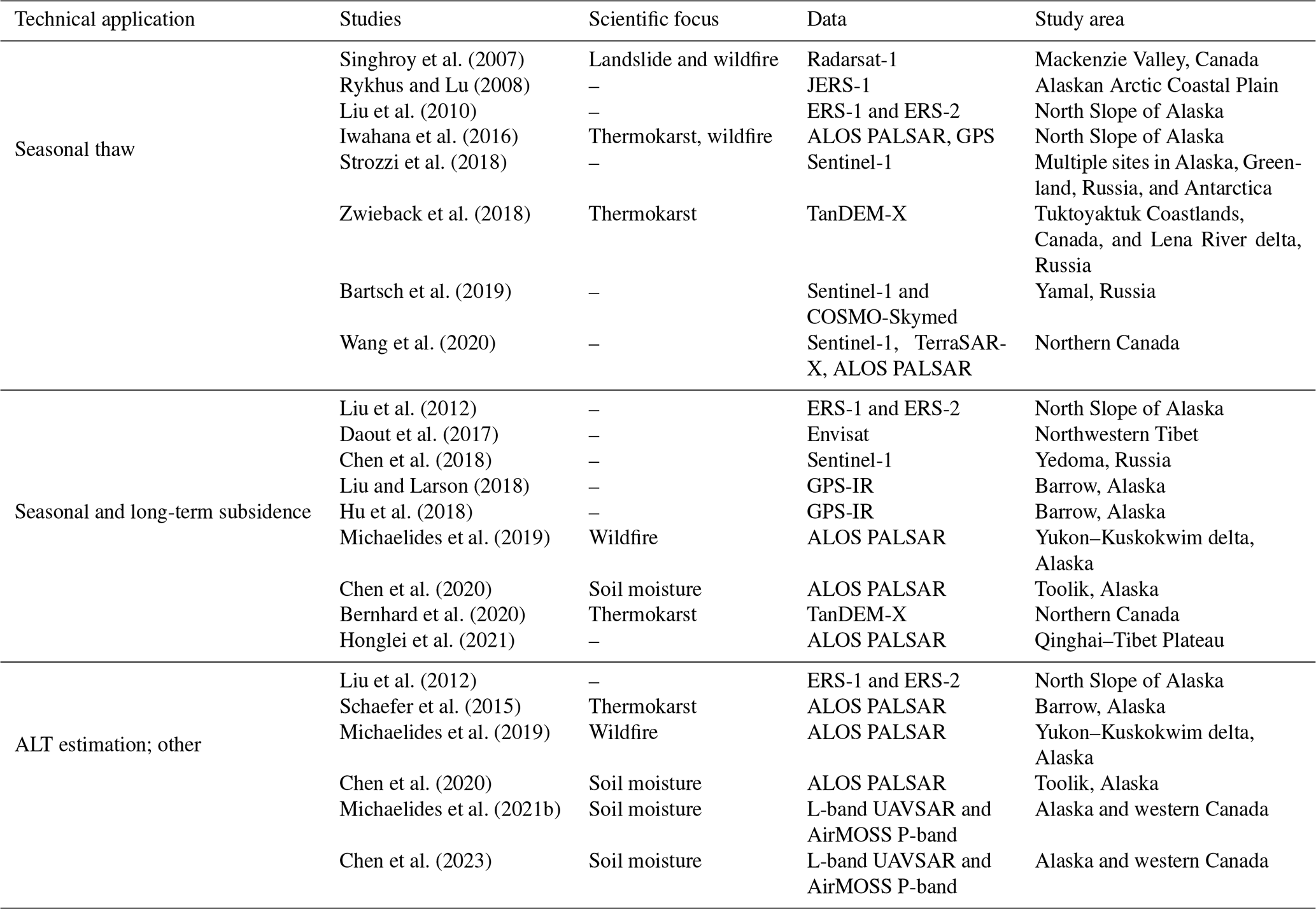
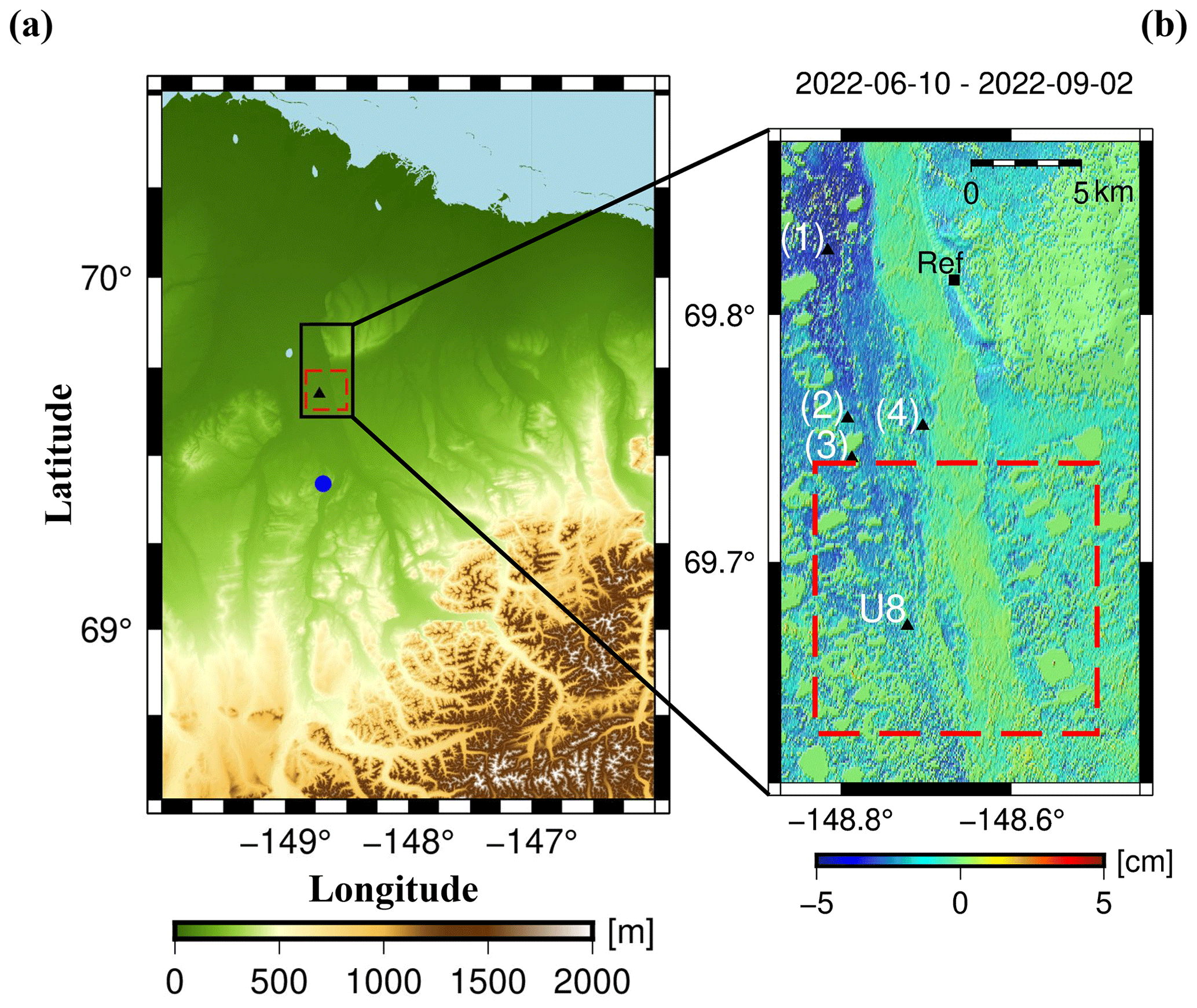
Figure 1(a) DEM including the study area (black box) in northern Alaska. The black box is expanded in Fig. 1b; the red boxes outline focused test area shown in Fig. 5. The black triangle shows the CALM site (U8) where ground-based measurements of ALT are available. The blue circle represents the location of the closest meteorological station (Sagwon). (b) Line-of-sight (LOS) displacement of the study area from 10 June 2022 to 2 September 2022 as measured by InSAR. Negative values mean displacement away from the satellite, and positive values mean displacement towards the satellite. The DEM relief map is shown in the background. Triangles show the location of the CALM site and the displacement time series shown in Fig. 3. The black square represents the reference point used for InSAR analysis.
The Alaskan North Slope is bounded by the Brooks Range to the south and southeast and the Arctic Ocean to the north. Our main study site on the North Slope is a 15 km × 30 km area in the vicinity of the Sag river and Dalton highway (69.68° N, 148.7° W; Fig. 1). It is ∼50 km south of Prudhoe Bay and ∼130 km north of the Brooks Range, located in the continuous-permafrost region of Alaska, with more than 90 % permafrost coverage (Jorgenson et al., 2008).
Our study site includes the Circumpolar Active-Layer Monitoring (CALM) site U8. The CALM program is designed to monitor the active layer and permafrost sensitivity to climate change over extended periods, typically spanning multiple decades (Brown et al., 2000). CALM site U8 has recorded ALT since 1996. The site encompasses a 1 ha area containing 121 sample square arrays, each measuring approximately 10 m horizontally. It is located 88 m above sea level, is relatively flat, and lies within an inner coastal plain with river terraces. The site has an organic layer that is ∼ 23 cm thick and that is usually water-saturated during thaw season. U8's vegetation coverage is classified as graminoid-moss tundra, graminoid prostrate dwarf shrub, and moss tundra. Its soil texture is classified as predominantly sand, gravel, and peat. The soil taxonomy is Ruptic–Histic–Aquorthel (Ping et al., 2015; Staff, 1999), i.e., a poorly drained, occasionally to frequently water-saturated soil with a significant amount of organic matter (https://www2.gwu.edu/~calm/data/webforms/u8_f.htm, last access: 29 August 2023). A 12 km × 12 km test site around U8 (red box in Fig. 1) is used for focused studies of ALT estimation based on our InSAR-derived displacement estimates during thaw season.
The circumpolar Arctic vegetation map (CAVM) at this location describes graminoid and prostrate-dwarf-shrub vegetation 5–10 cm in height. This vegetation structure is favorable for shorter-radar-wavelength radars, such as Sentinel-1's C band (∼5.5 cm wavelength), for purposes of retaining phase coherence, but it also suggests that accounting for vegetation height will be important to assess seasonal and longer-term elevation changes in this area.
4.1 InSAR data processing
4.1.1 Data and material
We used the Alaska Satellite Facility's Hybrid Pluggable Processing Pipeline (HyP3) software to form interferograms from Sentinel-1 SAR data (Hogenson et al., 2020). HyP3 uses the Copernicus GLO-30 digital elevation model (DEM) for scene co-registration and topographic phase corrections (ESA, 2021). Interferograms were filtered using the adaptive phase filter in Goldstein and Werner (1998). Individual interferograms were unwrapped using a minimum-cost-flow algorithm (Chen and Zebker, 2002) and geocoded to a 30 m grid spacing. We used the open-source Miami InSAR time series software in Python (MintPy) to generate line-of-sight (LOS) displacement time series from the unwrapped and geocoded interferograms (Fattahi et al., 2016; Yunjun et al., 2019). Interferograms with high spatial coherence and short time intervals between scenes were chosen to avoid decorrelation and phase-unwrapping errors. Phase-unwrapping artifacts occur in permafrost regions when disconnected wetlands and large seasonal deformation preclude smooth unwrapping of the phase (e.g., Strozzi et al., 2018). Noisy interferograms were removed from the time series and seasonal-amplitude inversion processes (Sect. 4.3.2). Geocoded LOS displacement data for active-layer thickness estimation were then extracted for the study area.
Significant changes in scattering characteristics are expected during the freeze season when the surface is covered with snow and ice; hence, we focus on the summer thaw season. Variations in soil moisture can also significantly affect coherence. To mitigate this possibility, we looked for noisy interferograms, which could be partly due to such moisture changes, and excluded these from our analysis. We employed two criteria to assess noise. First, we manually reviewed the interferograms and eliminated noisy ones. Second, we assessed the spatial coherence of the chosen interferograms to ensure they all had high coherence. Note that data were collected at a time where soil moisture was likely to be retained: the period that begins immediately after snowmelt, when the soil column is saturated, and that ends near the end of thaw season, when the soil column may still be wet due to the complete thawing of any residual ice in the active layer. We focused our study on the June to September time frame using Sentinel-1 SAR images with a 12 d revisit interval and descending geometry for the years 2017 to 2022 (Table S1 in the Supplement). Available meteorological data suggest no anomalous drought periods during these years.
4.1.2 Reference point selection
InSAR measures phase differences between SAR observations in space and time. To relate these phase difference measurements to surface displacement, a reference location with assumed or known displacement is required, with high temporal coherence (>0.8) to avoid introducing noise into the time series. In most permafrost regions, rock outcrops are a good reference as they can be assumed to show only minimal displacement. However, they may not be available for all regions. Liu et al. (2010) point out that river floodplains usually have well-drained sandy soils and, hence, tend not to experience significant frost heave. They may be used as reference points if they are not within a river channel, which can undergo large elevation changes from erosion and/or deposition events (see Fig. S3 in the Supplement). Figure 1b shows our reference point, a rock outcrop which remains coherent (temporal coherence ∼0.95) during the 2017 to 2022 thaw seasons.
4.1.3 Atmospheric-delay correction
Atmospheric effects are one of the main error sources in the InSAR process (Meyer et al., 2006). While InSAR data can be affected by both the ionosphere and the troposphere, here, we focus on tropospheric effects as ionospheric impacts are less pronounced in C-band data (Meyer, 2011). Tropospheric phase impacts can be modeled as follows (Ding et al., 2008):
where ϕ is the phase of a SAR image, d is the range from satellite to surface, δd is the tropospheric propagation delay, and λ is the radar wavelength. Tropospheric phase signals in InSAR data can be caused by two processes: changes in the atmospheric stratification and turbulent mixing. The stratified component typically correlates with topography (Hanssen, 2001) and may be estimated and then removed based on delay–elevation correlations (Doin et al., 2009). The turbulent component is usually much less than the stratified component but is uncorrelated in time and space and, hence, is harder to predict or measure. According to Eq. (1), if the atmospheric propagation conditions at the time of SAR acquisitions are not the same () then tropospheric phase components will be introduced, contaminating the true displacement signal. Applying atmospheric corrections to C-band radar images can improve the signal-to-noise ratio, especially when there is a considerable height difference between the study area and reference point. We applied the atmospheric correction model described in Jolivet et al. (2011, 2014) using ECMWF Reanalysis (ERA-5) datasets (Hersbach et al., 2020). This approach mainly reduces the stratification component of the tropospheric delay.
4.2 ICESat-2 data processing
To validate our InSAR measurements of thaw season subsidence, we used independent lidar elevation data from the ICESat-2 satellite (Martino et al., 2019). The ATLAS (Advanced Topographic Laser Altimeter System) lidar on ICESat-2 uses a multi-beam photon-counting laser operating at 532 nm, i.e., the green portion of the electromagnetic spectrum. The surface range is determined by the travel time of each detected photon. When coupled with the satellite's position, the range data provide accurate geolocation of the surface, in this case referenced to the WGS-84 ellipsoid. With a laser repetition rate of 10 kHz, pulses occur approximately every 70 cm on Earth's surface. Each footprint is about 13 m in diameter. Beam pairs, with different energies to adjust for surface reflectance, are spaced about 3.3 km apart across tracks, forming six tracks with beams in each pair separated by 90 m. The ranging precision for flat surfaces is expected to have a standard deviation of around 25 cm, primarily influenced by ATLAS timing uncertainty (Neuenschwander et al., 2019).
The ATL08 product algorithm is designed to extract terrain and canopy heights from vegetated surfaces using the geolocated photons (Neuenschwander et al., 2019). We used the “h_te_best_fit” parameter, which estimates terrain height by fitting a plane to along-track points in each 100 m segment and reports the height of the middle of the fitted plane (Neuenschwander and Magruder, 2019; Neuenschwander et al., 2021), reducing the impact of random errors. The height of the terrain midpoint is calculated by choosing the best fit among three models: linear, third-order, and fourth-order polynomials applied to the terrain photons. This allows for interpolation of the elevation at the midpoint of the 100 m segment (Neuenschwander and Magruder, 2019; Neuenschwander et al., 2021; Neuenschwander and Pitts, 2019). The standard deviation of terrain points around the interpolated ground surface within the segment is one measure of surface roughness. Neuenschwander and Pitts (2019) provide additional details describing the ATL08 algorithms. ATL06 is an alternate-product algorithm, optimized for ice surfaces, and it has been used in some permafrost studies (e.g., Michaelides et al., 2021a) (see Supplement).
While the nominal temporal resolution of ICESat-2 data is 91 d, cloud cover often limits the amount of usable data in Alaska (e.g., Neuenschwander and Pitts, 2019). Two repeat track observations were available in our study area, acquired on 8 June 2021 and 6 September 2021. Due to pointing-related uncertainty, observations are not always repeated in expected locations, which amplifies the height uncertainty. To address this issue, we divided the study area into 50 m grid cells and assigned each observation from the 8 June 2021 and 6 September 2021 repeat tracks to one of those grid cells. Figure S3 shows the height difference between all reported terrain observations (ATL08) in the study area from the same location between 8 June 2021 and 6 September 2021. In the limited area where both InSAR and ICESat-2 data are available, we used the ICESat-2 data to compare to our InSAR results (Fig. 3 and Supplement).
4.3 Active-layer-thickness estimation model
To relate the InSAR observations to ALT, we assume that the measured LOS displacements are predominantly due to vertical motion (negligible horizontal motion) and that this vertical motion is caused by thawing ground ice in the active layer. The assumption of negligible horizontal motion is justified because, over the short data time interval, the technique is not sensitive to long-term tectonic motion. Displacements from the M 6.4 August 2018 earthquake, ∼130 km east of the study area (USGS hypocenter at 69.576° N, 145.291° W; depth of 15.8 km) are negligible. Most surface motion in the thaw season therefore likely reflects thawing ground ice. We project the LOS displacements into the vertical direction using the local incidence angle (θ) for each radar pixel (see Eq. 3). We follow the simplified Stefan solution to estimate the depth of thawing in the soil (Nelson et al., 1997) aided by field-observed air temperature data. We also assume that subsidence can be related to a simple thaw index, for example, the accumulated degree days of thawing (ADDT). Our procedures are virtually identical to those described in Liu et al. (2012) and Schaefer et al. (2015), with the exception that we do not estimate multi-year subsidence and do not average ALT across multiple thaw seasons. This enables us to directly compare our space-based estimates with yearly ground truth estimates from CALM site U8 and to evaluate inter-annual changes in ALT.
4.3.1 Accumulated degree days of thawing calculation
To calculate ADDT, we use the NOAA Climate Data Online (CDO) tool to find nearby meteorological stations. The closest station is ∼30 km south of our test area (name: Sagwon, Fig. 1a). We assume that our test area has the same temperature trend as this station for the 2017 to 2022 thaw seasons. We define the first and last days with temperature >0 °C as the first and last days of the thaw season. ADDT is defined by the following equation (Riseborough, 2003):
where αs is the duration of the thawing season in days. Ts is surface temperature (°C), Tf is equal to the freezing point of 0 °C, and is daily mean surface temperature. Due to the lack of in situ surface temperature data, we set using air temperature observations.
4.3.2 Seasonal-amplitude inversion
The relationship between the seasonal vertical surface displacement magnitude and ADDT can be written as follows (Liu et al., 2012; Schaefer et al., 2015):
where Di is the vertical-displacement estimate for a given pixel in the ith interferogram; θ is the local incidence angle at that pixel calculated from nadir; and E is the amplitude of the seasonal vertical-displacement estimate, which reflects physical parameters such as soil thermal conductivity, latent heat of fusion, soil density, and relative water content (Nelson et al., 1997). A1,i and A2,i are normalized accumulated degree days of thawing at the first and second acquisition date. ε is an error term that captures model deficiencies, noise, and other unknown error sources. We do not consider secular (long-term) displacement signals in Eq. (3) because we analyze the thaw seasons of 2017 to 2022 separately. This is the major difference between our approach and those described in Liu et al. (2012), Schaefer et al. (2015), and Michaelides et al. (2019), where seasonal and inter-annual trends were estimated simultaneously.
We can rewrite Eq. (3) in matrix form considering the interferograms listed in Table S1 to estimate E using least squares for separate thaw seasons:
4.3.3 Active-layer-thickness inversion
If we assume that the seasonal vertical surface displacement amplitude E is caused only by thawing ice and corresponding volume reduction, we can write E as a function of physical properties such as soil porosity, soil moisture fraction, and density of ice and water through a vertical profile from the surface to the depth of the active layer (Liu et al., 2012; Schaefer et al., 2015):
The variables ρw and ρi in Eq. (5) are the density of water and ice (kg m−3), respectively. P(z) is the soil porosity, which is a function of depth and depends on soil content, and S(z) is the soil moisture fraction of saturation. Following Schaefer et al. (2015), we assume S(z)=1, which means that the active layer is fully saturated, and saturation does not change with depth.
4.3.4 Porosity model
Following earlier authors, we assume that soil in the active layer consists of organic matter and mineral soil, with porosity decreasing exponentially with depth due to decreasing organic matter. There is one active CALM site in our test area: U8 (Fig. 1b). This site is described as having an organic-layer of thickness 23 cm, consisting mainly of peat plus sand and gravel (Sect. 3). We applied the formulation introduced by Liu et al. (2012) and assume that it is the weighted average of organic and mineral matter.
In the above, P is the porosity, and forg is defined as the organic soil fraction by Schaefer et al. (2009) as follows:
In Eq. (7), Morg and ρorg are the simulated masses of organic matter and organic soil density in a given layer of soil, respectively. Morg_max and ρorg_max are bulk organic matter mass and bulk density for pure organic soil, respectively. We set Porg=0.95 based on the model from Bakian-Dogaheh et al. (2022). The porosity of mineral soil then depends on the sand fraction of soil. To estimate Pmin we used the porosity–sand fraction relation provided in Liu et al. (2012):
We used Global Land Data Assimilation System (GLDAS) soil parameters with 0.25° spatial resolution to extract the soil sand fraction (Rodell et al., 2004). We set Pmin=0.488 and ρorg_max=130 kg m−3 for the bulk density of peat (Grigal et al., 1989; Hossain et al., 2015). As mentioned earlier, to formalize with depth, we assume that the organic matter amount decreases exponentially with depth:
where k is an empirical constant (m−1), set to 5.5 (Liu et al., 2012; Jackson et al., 2003). To retrieve B, we use the simulated mass of organic matter (Morg: total soil carbon content) from Johnson et al. (2011) and Mishra and Riley (2012) and ensure that the total carbon mass is conserved:
We set Morg=70 kg m−2 (Johnson et al., 2011; Mishra and Riley, 2012). The spatial divergence of total soil carbon content for the 0–100 cm depth range is large in Arctic tundra regions considering the vegetation type. Mishra and Riley (2012) and Johnson et al. (2011) estimate the total soil carbon around our study area to be 60–80 kg m−2 and 50–70 kg m−2, respectively. Root depth is the maximum observed ALT at a given site since roots cannot penetrate solid ice. Here, we set the maximum root depth to be 1.1 m because the maximum observed ALT at site U8 is reported to be ∼1.1 m for 2022. Then we solve Eq. (10) for B and replace it in Eq. (9). Figure 2 shows the relation between porosity and depth in a mixed soil. We set P=0.95 for the first ∼23 cm depth, reflecting organic matter thickness. After 23 cm depth, the porosity decreases exponentially, reaching its minimum near the top of the frost table. Finally, we put all equations into Eq. (5) and use a numerical-bisection algorithm to solve for the upper integral limit, ALT. We set the accuracy of bisection to be at the millimeter level.
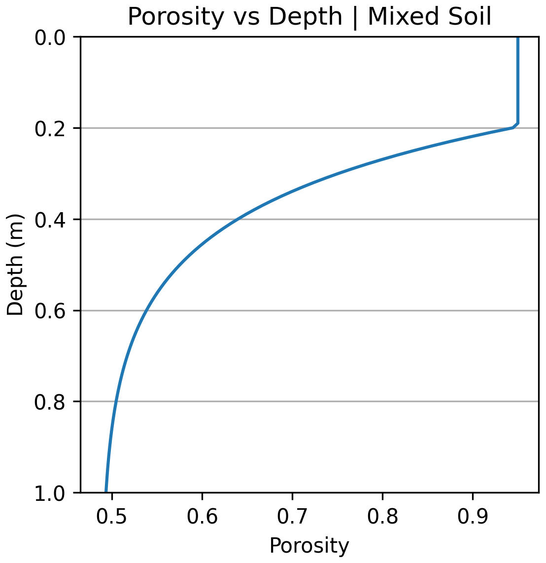
Figure 2Depth–porosity model used in this study assuming a mixture of organic and mineral matter.
5.1 Estimating seasonal vertical displacement
Figure 3 shows displacement time series for the four test locations shown in Fig. 1b. All four locations show subsidence during thaw season. The maximum amplitude of subsidence ranges from 20 mm (location 4) to 60 mm (location 1). In 2021, the subsidence amplitude was small and similar among the four locations (∼20 mm). The subsidence rate is approximately constant during the thaw season. The root mean square error (RMSE) of the linear fit to the displacement data is less than 7 mm at all four locations over all 6 years. The maximum subsidence rate observed during the short (∼3–4 months) thaw season is ∼18 mm per month.
Note that we do not attempt to connect our displacement time series across adjacent years. The freezing process, consequent frost heave, and deep snow at these sites during winter make phase connection difficult due to loss of coherence (e.g., Strozzi et al., 2018). Nevertheless, our approach can still be used to assess long-term (multi-year) changes in permafrost, as shown in Sect. 5.3.
Figure 4 shows the seasonal subsidence rates at the four locations over the 6-year test period. No clear long-term trend is observed. Location (1) has the largest rate variation, from 4 mm per month in 2018 to 18 mm per month in 2020. Location (3) has the minimum rate variation at 5 mm per month in 2017 to ∼10 mm per month in 2021. We do not observe spatial correlation between subsidence rates at the various locations. For example, location 1 shows the fastest subsidence, with high rates in 2017, 2020, and 2022 but much smaller rates in 2018, 2019, and 2021. Location 2's fastest subsidence occurs in 2019, while the fastest rates for location 3 and location 4 occurred in 2019 and 2021.
5.2 Validation of InSAR surface displacement estimates with ICESat-2 data
We used the ICESat-2 ATL08 data product to compare with our InSAR time series of relative height change for the 2021 thaw season (Fig. 3). Comparisons using the optical lidar data are primarily limited by cloud cover; however, all four of our test locations had suitable ICESat-2 data at the beginning and end of the 2021 thaw season. To minimize the effect of systematic errors, we used repeat data from the same reference ground track (RGT =1150) and considered only elevation change during thaw season, referencing the height of the second acquisition (end of thaw season: 6 September 2021) to the first (beginning of thaw season: 8 June 2021). The height of the first date's lidar data is assigned “zero elevation” to agree with the InSAR estimate. This is a reasonable assumption because the two datasets have similar start dates in 2021, namely 8 June for ICESat-2 and 3 June for SAR.
Figure 3 shows that, with these assumptions, the lidar and radar approaches agree well. Since the two approaches to elevation change estimation are independent, their agreement is a strong validation of the InSAR approach despite being limited to a small number of test cases. The agreement between the two approaches also suggests that our reference point for the InSAR data experiences negligible change during the study period. Reference point selection for InSAR is difficult in remote permafrost regions as most areas undergo subsidence during the thaw season. ICESat-2 data, when available, could help in this regard but will be limited by pointing errors, cloud cover, and density of the vegetation canopy.
We also tested the utility of ICESat-2's ATL06 data product (“h_li”) (Smith et al., 2019), described in the Supplement. For this test, we expanded the comparison to a larger number of sites and dates but otherwise used the same general procedures as for the ATL08 product. For our original four test sites, the ATL08 product shows better agreement with the InSAR data (Figs. S4–S5). In our larger study area, 78 cells reported both ATL08 and ATL06 data. For these cases, the two products are equivalent (within 1 cm height difference) in 9 % of cases and agree within 10 cm in 61 % of cases (Fig. S4). Including the four original test sites described above, for the 15 cases where InSAR and ICESat-2 products were available, ATL08 shows better agreement with InSAR in 8 cases, while ATL06 shows better agreement in 7 cases. In relatively flat areas, both data products show similar performance. The larger footprint of the averaged ATL08 data product (100 m) compared to ATL06 (40 m) may also be advantageous given the high spatial variability of ALT (see Sect. 5.3). The Supplement also includes a description of the formal uncertainties associated with both the ATL06 and ATL08 data products.
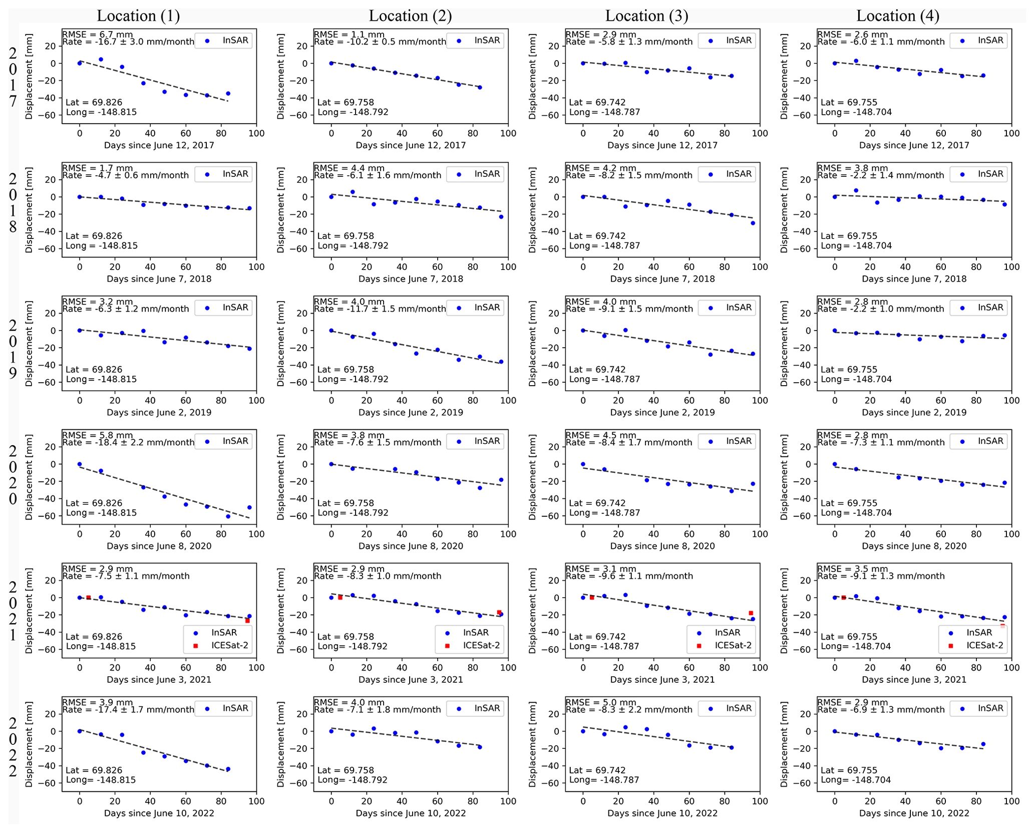
Figure 3LOS displacement time series for four test locations (black triangles in Fig. 1b) with respect to the first SAR acquisition in the thaw season. Dashed black lines are the best-fitting regression lines for InSAR LOS displacement only. The rate and RMSE of fitted lines are shown in the top left of each sub-figure. Red squares in 2021 show the ICESat-2 ATL08 terrain height product. The latitude and longitude of each analyzed location are shown in the bottom left of each panel. Note that subsidence only occurs during the thaw season and not throughout the entire year.
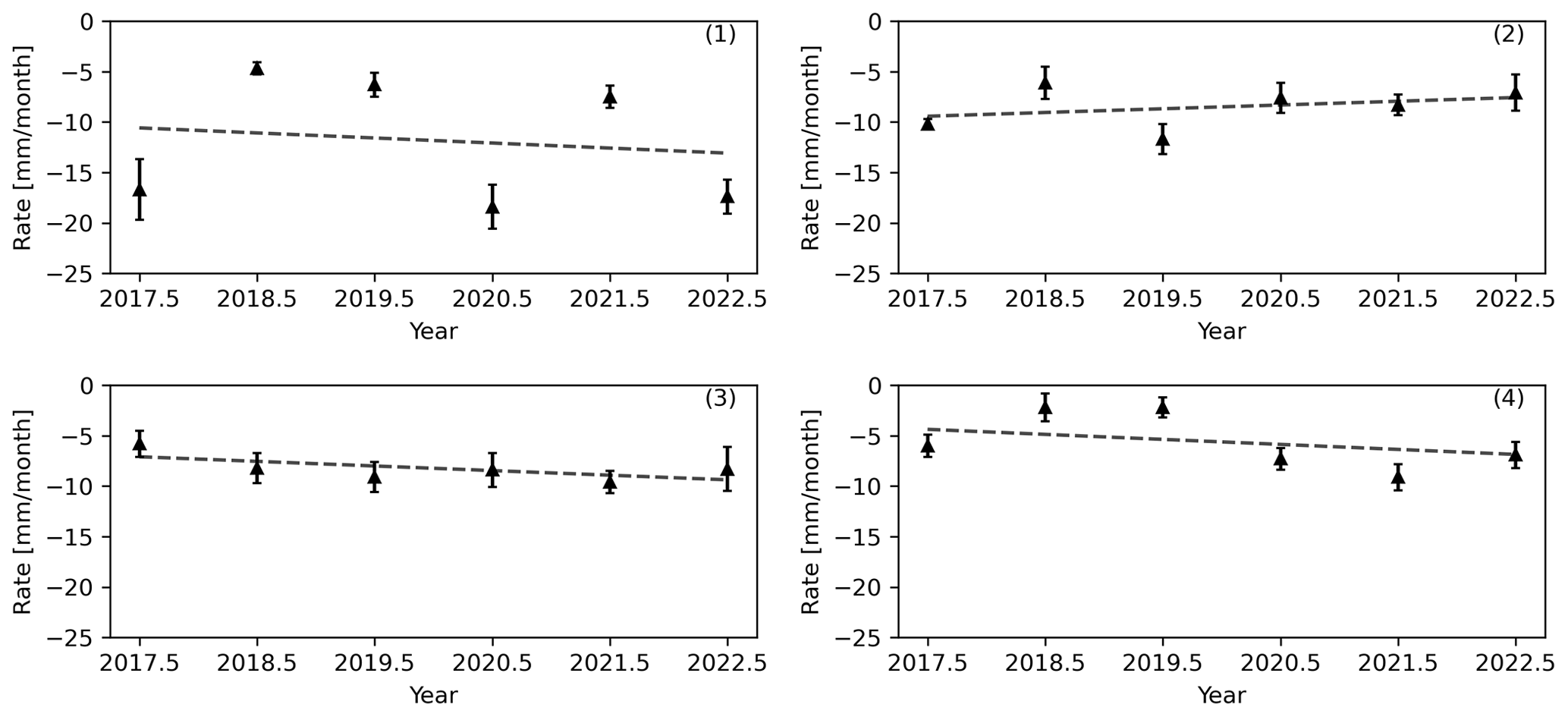
Figure 4Rate comparison of LOS displacement during the summer thaw season for the locations shown in Fig. 1b. The rate and an error bar are from the linear fitted line (see Fig. 3).
5.3 Active-layer thickness estimation and validation
Figure 5 shows the seasonal vertical-displacement amplitude and its RMSE calculated from Eq. (4) and the estimated ALT from 2017 to 2022 in our test area (red box in Fig. 1) using procedures described in Sect. 4.3. The minimum ALT occurred in 2018 and 2021. The maximum ALT occurred in 2019 and 2020. The variation in these estimates may, in part, reflect uncertainty in the thaw season length. Thaw season usually starts around 20 May and ends around 20 September, but the accumulated degree days of thawing differ each year. Sagwon station data for this time period show that maximum and minimum ADDT occurred in 2019 and 2018, respectively (Table 2). The overall pattern of ALT remained the same in 2017, 2018, 2021, and 2022 but differed in 2019 and 2020. Maximum ALT occurred to the west and southwest of site U8. This was also true in 2019 and 2020, but spatial variation was higher than other years.
Table 2Thaw onset and end and ADDT for 2017 to 2022 based on Sagwon station (Fig. 1).
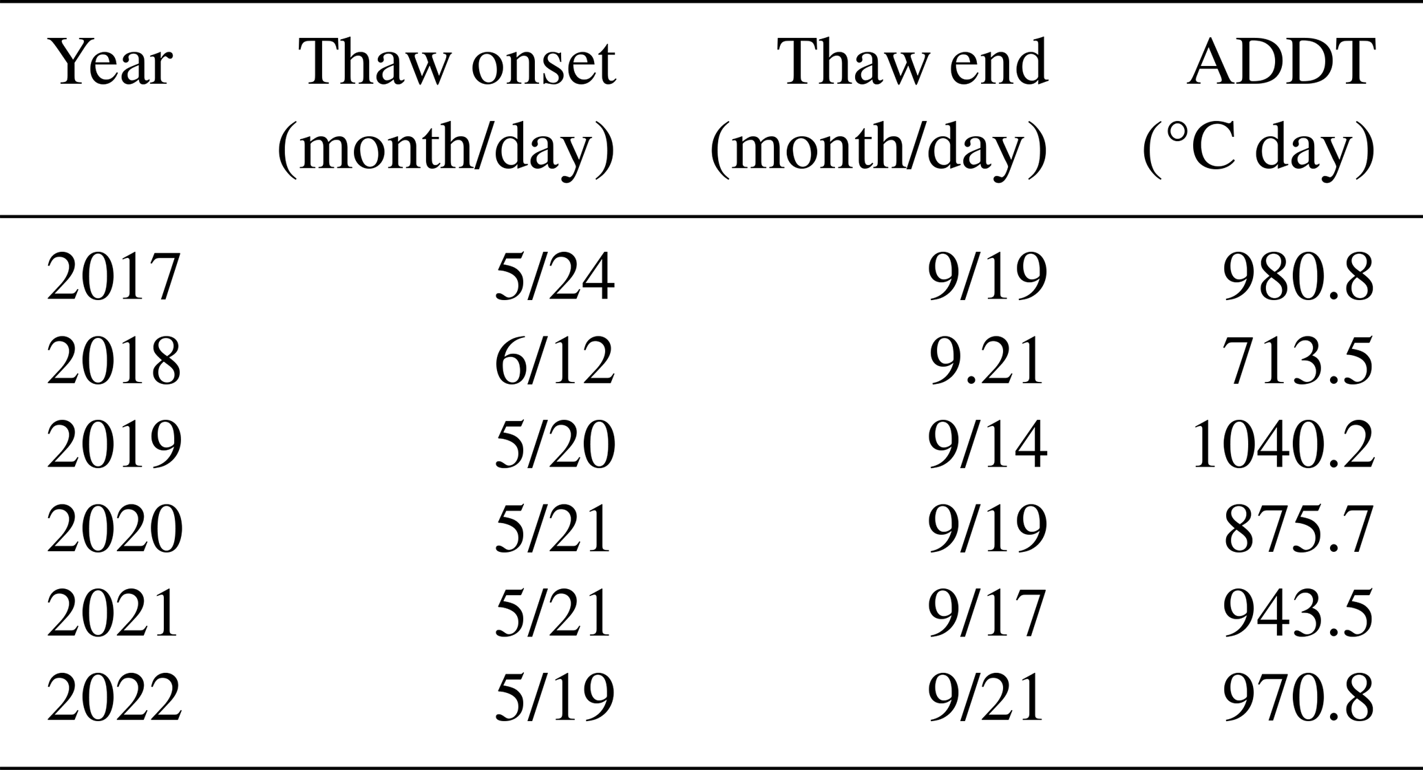
ALT, in some areas, showed a deeper-than-usual pattern in 2019 and 2020 but recovered in 2021 and 2022. For example, an area a few kilometers southeast of U8 showed high variability in 2019 and 2020 but a shallow ALT before (2017 and 2018) and after (2021 and 2022). A deeper ALT in 2019 correlates with ADDT. However, a deeper ALT in 2020 and a shallower ALT in other years does not clearly correlate with ADDT – 2020 was the second coolest thaw season in our study period, with ADDT = ∼876 °C day (Table 2).
We can compare our results with in situ data. CALM site U8 is a 1 ha area with 121 samples in a square array. Each sample area is 10×10 m. Its ALT has been observed at the end of the thaw season since 1996. Thaw depth is measured by pushing a metal rod into the soil to refusal, assumed to represent the top of the permanently frozen layer. ALT is not reported if the probe intersects ponded water or rocks. The mean of all 121 ALT measurements and the corresponding RMSE values are reported. Our approach for reporting InSAR-derived ALT is similar. The pixel closest to U8 and adjacent pixels within 50 m in the east–west and north–south directions are defined. We report the mean of these pixels and their RMSE values for comparison with in situ data.
Figure 6 shows ALT data around the U8 CALM site for different years. Our estimated ALT agrees within uncertainty with the in situ data for all 5 of the years when data are available. In situ ALT is not reported for 2020. This agreement suggest that our assumptions about model parameters, based on available in situ data and the published literature, are reasonable.
Chen et al. (2020) estimated ALT and volumetric water content for large areas in Alaska, including the U8 CALM site, using L-band UAVSAR and AirMOSS P-band polarimetric SAR, respectively. Their result is in good agreement with the in situ data and this study considering joint uncertainties. Data-processing details are provided in Michaelides et al. (2021b) and Chen et al. (2023).
To assess the agreement between in situ data and estimated ALT, we follow Liu et al. (2012) and use Eq. (11) to evaluate whether a given year’s InSAR-based estimate of ALT is consistent with the in situ observation given its data uncertainty:
where the numerator is the residual between in situ and InSAR-based ALT, and the denominator is the reported in situ data uncertainty; r2 values lower than 1 indicate good agreement. Except for the 2017 estimate, with r2=2, all other years have r2 less than 1. The estimated ALT in 2022 shows the best agreement with r2=0.3. Figure S2 gives more details.
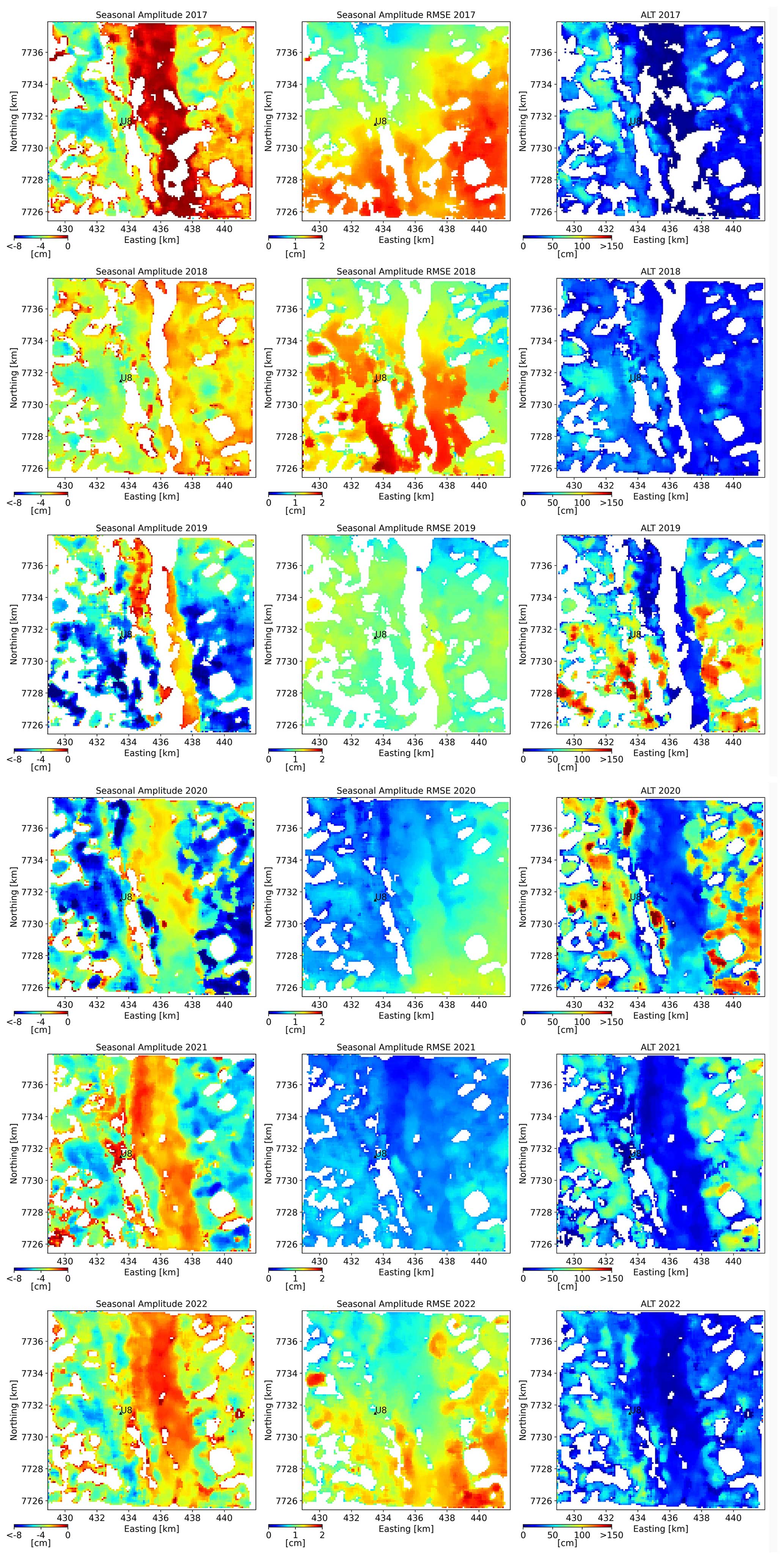
Figure 5Estimated seasonal amplitude, its RMSE and ALT for study area (red box Fig. 1a, b) from 2017 to 2022. Black triangle shows location of CALM site U8. White areas represent low coherence which are masked out in the model calculations. The Sag river runs south to north in the center of each panel (see Fig. S3).
Our results and the in situ data suggest that ALT exhibits high spatial variability. It is generally assumed that ALT depends on parameters such as ADDT, precipitation, and local topography, the latter reflecting its influence on soil moisture and aspect. Our results show a moderate correlation with ADDT but no correlation with precipitation, although the latter could reflect the limited spatial resolution of the available data.
The influence of local topography on ALT can be tested by examining the available high-resolution in situ data. Data from the U8 CALM site provide an excellent opportunity to investigate both the spatial and temporal variability of ALT. Over this small area, we expect that local topography will show minimal year-to-year variation. Figure 7 shows ALT variation over an 11×11 square array of sample points, with each point sampling an area of 10×10 m. Data are available for the period between 1996 and 2022, with a gap in 2020. The location is described in local coordinates. We also show the RMSE of each grid point based on its average over this time period and a time series of ALT for three representative points in the array.
Even over this small area, we see no significant spatial or temporal pattern in ALT over the quarter-century period of available data. At least for this example, the influence of local topography appears to be minimal, although we cannot preclude microtopographic (less than 10 m) effects that vary over time.
The Mann–Kendall test was employed to evaluate this in a rigorous way. The test determines if a significant monotonic trend is present for either increasing or decreasing ALT at each grid point. Data spanning from 1996 to 2019 were analyzed due to the absence of data in 2020. To maintain consistency and account for possibly significant temporal variations in ALT, data from 2021 and 2022 were excluded. The null hypothesis was rejected for 31.4 % of the cells; the remaining 68.6 % of cells do not show a statistically significant trend. In other words, only 38 out of 121 cells had a significant increasing or decreasing ALT trend. Among these 38 cells, 35 cells showed an increase in active-layer thickness over the sample time period. The maximum RMSE of the cells is ∼20 cm. Variation in the same grid cell over 2 consecutive years reaches as high as ∼60 cm. Since air temperature (related to ADDT) and precipitation are unlikely to vary significantly over this 100×100 m area and since the overall morphology is unlikely to vary significantly over this time period, other factors must explain the variation in ALT. Given that our estimated ALT aligns well with in situ ALT (Figs. 6, S2) and that the long-term in situ ALT measurements (2002–2022) show no correlation with ADDT and precipitation (Fig. 8), we suggest that other factors are likely to be influencing the results. Micro-topographic effects, temporal changes in sub-surface moisture flow, soil organic content, and vegetation growth and decay are possible factors. Nelson et al. (1998), Nelson et al. (1999), and Hinkel and Nelson (2003) conclude that in situ ALT shows Markovian behavior with high spatial and temporal variations.
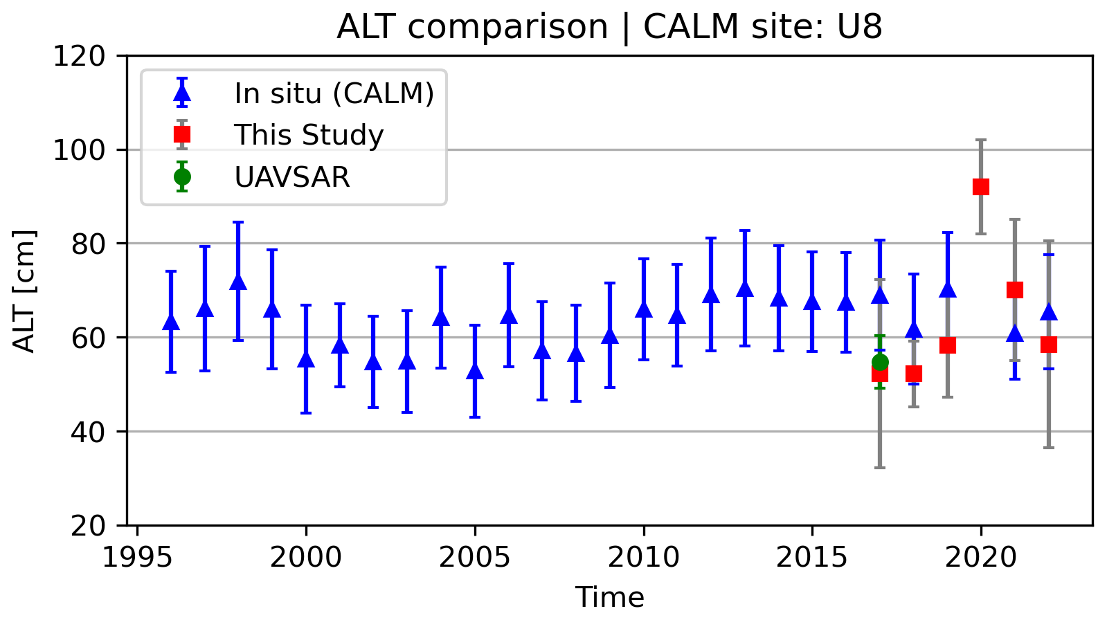
Figure 6ALT comparison at CALM site U8. Blue triangles represent the average in situ ALT from manual mechanical probing across all grid cells from 1996 to 2022 (https://www2.gwu.edu/~calm/data/north.htm, last access: 29 August 2023). The green circle is the estimated ALT for the closest pixel to U8 using airborne L- and P-band SAR images (Chen et al., 2022). Red squares (this study) are the average estimated ALT for pixels within 50 m of U8. In situ ALT is not reported for 2020.
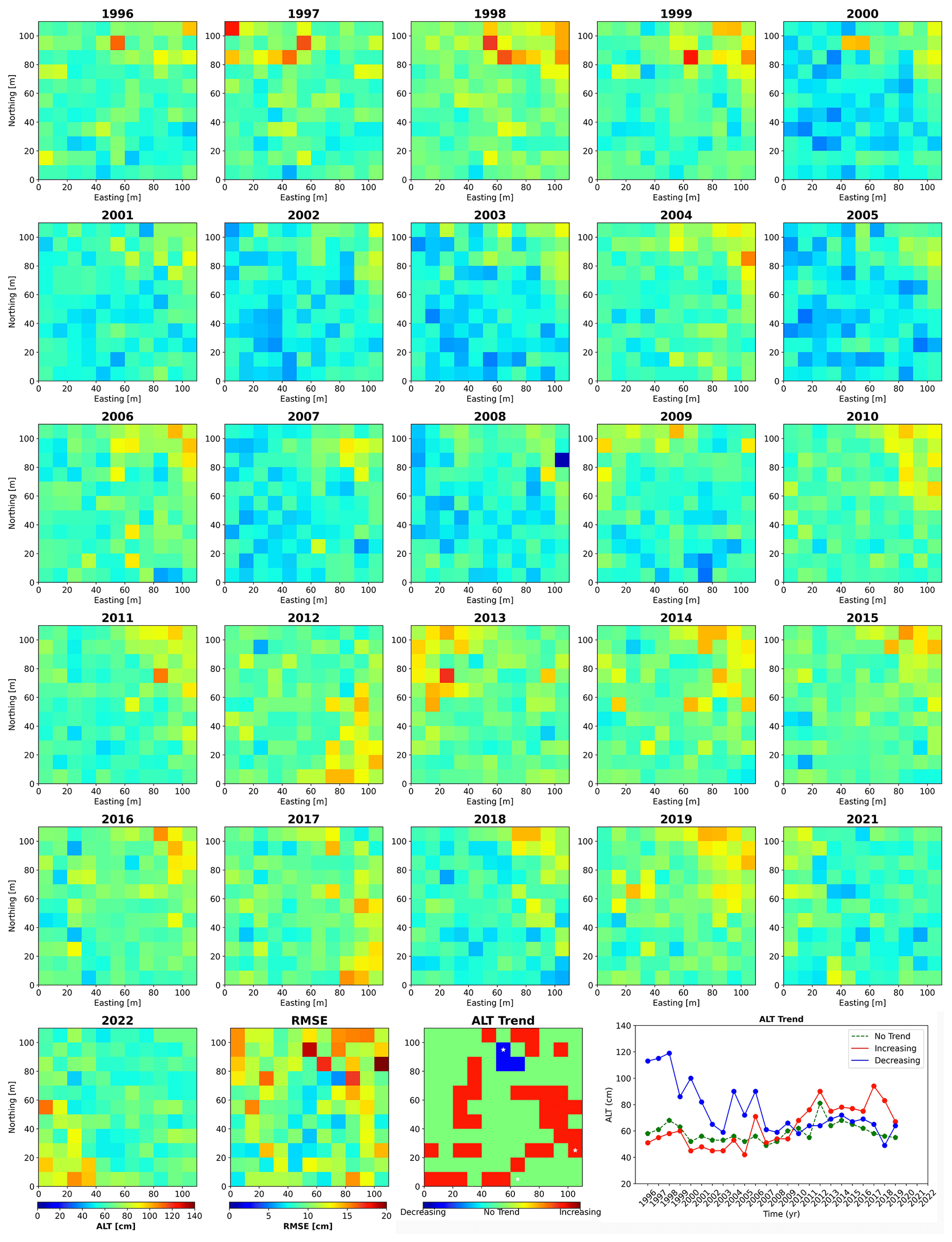
Figure 7ALT variation at CALM site U8, RMSE of each cell in relation to the annual average from 1996 to 2022, and ALT trend and ALT time series for three selected cells (10×10 m) shown by white stars.
5.4 Relation of meteorological parameters to active-layer thickness
We investigated correlations between in situ ALT and several meteorological parameters, including ADDT and precipitation, in thaw seasons from 2002 to 2022. ADDT and precipitation data are from the Sagwon meteorological station. Figure 8a shows the relation between ADDT and ALT. From Stefan's equation, we expect a positive correlation between ADDT and ALT. However, the correlation is weak (R2=0.42; Fig. 8b), suggesting the influence of additional factors. Precipitation may influence ALT, e.g., by advecting heat downward to promote permafrost thaw, but there are additional factors to consider. For example, an increase in soil moisture leads to a rise in the thermal conductivity of soil, potentially increasing the depth of the active layer during the thaw season. However, an increase in soil moisture also increases the total amount of heat required for thawing, promoting a shallower active layer. Clayton et al. (2021) showed that ALT has a positive correlation with volumetric water content (VWC) in the upper 12 cm of soil, a negative correlation with bulk VWC, and no statistically significant correlation with VWC in the upper 20 cm of soil. We also do not see a statistically significant correlation between ALT and precipitation, perhaps reflecting these opposing impacts (Fig. 8c).
We used simple regression analyses to relate ALT to several multi-parameter factors, including ADDT, precipitation, and accumulated degree days of freezing (ADDF) from the previous year. However, these did not improve the correlation. Perhaps other factors such as local elevation gradients (influencing local hydrology), vegetation type, or the previous year's snowfall need to be considered. It is also possible that some of the variability in our ALT estimates reflects variations in total ice content instead (Zwieback et al., 2024).
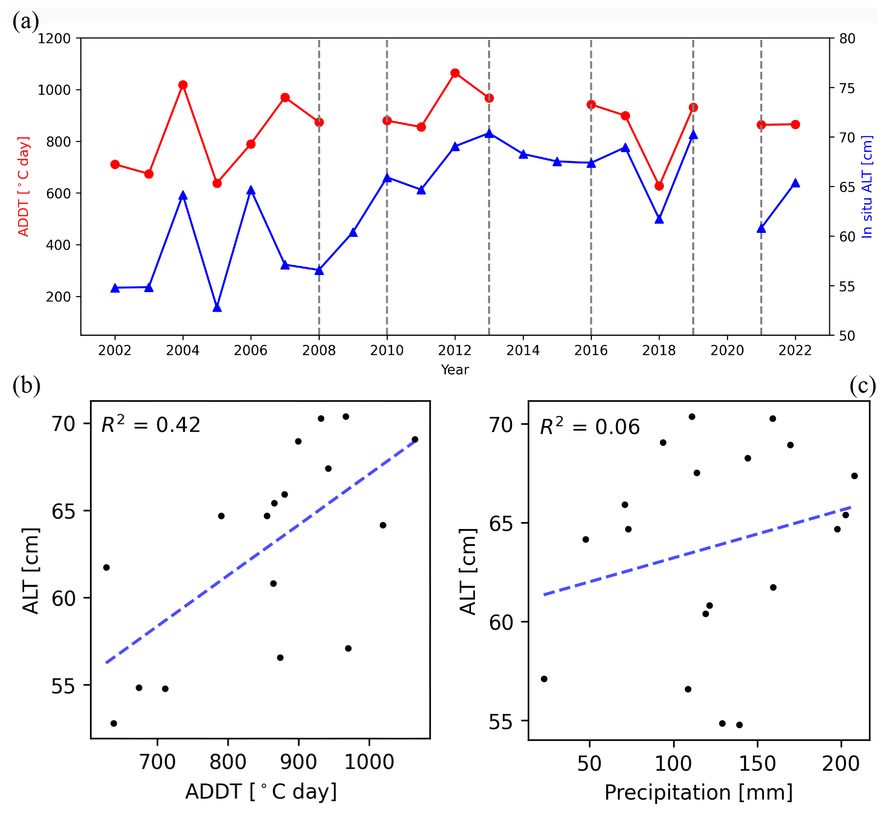
Figure 8(a) Relation between ADDT and ALT from 2002 to 2022 in CALM site U8 and at Sagwon station. Red circles show ADDT. Blue triangles show in situ ALT. (b) Scatterplot of ALT vs. ADDT. (c) Scatterplot of ALT vs. precipitation. R2 of relation is shown in top left of panels. ADDT and precipitation are calculated from 1 June to 1 September of each year to be consistent with ALT measurements.
5.5 Applicability to other regions
Alaska's North Slope is an optimum region for InSAR-based approaches to permafrost monitoring because of limited tree cover. We also tested our technique in a region with more extensive tree cover, the beta site of the APEX (Alaska Peatland EXperiment) project, located approximately 40 km southwest of Fairbanks (64.696° N, 148.322° W). This site is located in Alaska’s discontinuous-permafrost zone and has abundant black spruce up to 5 m in height. The technique was not successful as phase coherence was not maintained in successive SAR images, perhaps reflecting the relatively short wavelength (C band) of the Sentinel-1 SAR instrument (see next section). Average spatial and temporal coherence maps for these two sites are compared in Fig. S1.
5.6 Limitations and future research
Four aspects of our approach limit its utility and are an obvious focus for future research.
-
Decorrelation of InSAR phase is the main limitation of our technique. Accurate InSAR measurements require a high degree of coherence, a measure of the correlation in radar phase between the two SAR images. Decorrelation occurs due to temporal changes in surface scattering properties, changes in viewing angles, and noise in the SAR data (e.g., Schaefer et al., 2015). The C-band InSAR has demonstrated its ability to monitor deformation over continuous-permafrost regions at higher latitudes (see the “Previous work” section of this study). Wang et al. (2020) compared the efficiency of Sentinel-1 for monitoring permafrost deformation in discontinuous-permafrost regions. They concluded that Sentinel-1 InSAR time series perform effectively over permafrost landscapes mainly beyond the tree line, such as tundra, tundra wetlands, and less developed shrub–tundra areas. However, the outcomes and precision are less favorable in shrub–tundra and forest–tundra environments. Our results are essentially the same: temporal and spatial coherence in our main study area, north of the tree line near CALM site U8 (almost entirely free of trees, (https://www2.gwu.edu/~calm/data/webforms/u8_f.html, last access: 29 August 2023) are significantly better than those obtained in the discontinuous-permafrost region near Fairbanks, Alaska (Sect. 5.5). Significant decorrelation also occurred around CALM site U18 (∼15 km southwest of Fairbanks, Alaska) during the 2023 thaw season. Land cover here is open black-spruce forest (https://www2.gwu.edu/~calm/data/webforms/u18_f.htm, last access: 29 August 2023). Longer wavelengths, such as L band, may be more useful in densely vegetated terrains. The NISAR mission, scheduled for launch in 2024, with its L-band wavelength and repeat frequency of 6–12 d, should prove to be useful for more densely vegetated discontinuous-permafrost regions.
-
The spatial and temporal resolution of models that allow estimation of key ancillary parameters may limit accuracy in some regions, for example, soil parameters from the GLDAS model and atmospheric parameters from ERA-5. The spatial resolution of GLDAS's soil parameter model is 0.25°, an area that spans our entire study area in the Alaskan North Slope. The temporal resolution of ERA-5 is adequate, but its spatial resolution limits local analysis.
-
Accurate, dense, and widespread porosity–depth profiles would improve ALT estimation from remotely sensed data. In particular, empirical and statistical models of soil properties calibrated with in situ data could significantly improve radar-based ALT models (e.g., O'Connor et al., 2020; Bakian-Dogaheh et al., 2020, 2022, 2023).
-
Variations in soil ice content and non-linear thaw season subsidence time series need to be considered (Zwieback et al., 2024).
We used Sentinel-1 interferometric SAR data from 2017 to 2022 around CALM site U8 in northern Alaska to measure thaw season subsidence and to estimate active-layer thickness with a widely used physical model that exploits the volume difference between ice and water. Limited ICESat-2 lidar data are consistent with InSAR estimates of seasonal subsidence. We do not attempt to estimate long-term (multi-year) elevation change. Instead we estimate ALT at the end of each thaw season and compare its yearly evolution, avoiding issues of decorrelation of the radar signal over the winter season.
ALT estimates in our study area range from ∼20 cm to more than 150 cm, similarly to in situ measurements at the CALM site and previous remotely sensed estimates. Agreement with the later part of the quarter-century-long CALM time series is notable and suggests that annual ALT estimates from satellite InSAR can be effective at monitoring longer-term permafrost health, at least for Alaska's continuous-permafrost zone north of the tree line. However, the technique was not effective in the discontinuous-permafrost region of central Alaska near Fairbanks, reflecting decorrelation of the C-band radar signal, probably from heavy tree cover. At the northern study site, ALT shows high spatial and temporal variability in both the satellite and in situ datasets, sometimes changing dramatically between adjacent 10 m cells. Subsidence rate also varies significantly between closely spaced points, ranging from ∼2 to 18 mm per month at our northern study site during thaw season. The reasons for such high spatial and temporal variability in ALT are not clear and warrant further research.
Meteorological data from the NOAA climate data online tool (CDO) are publicly available at https://doi.org/10.7289/V5D21VHZ (Menne et al., 2012a, b). The Copernicus GLO-30 digital elevation model is publicly available through https://doi.org/10.5069/G9BG2M6R (OpenTopography, 2016). Sentinel-1 data are publicly available through the Alaska Satellite Facility (https://search.asf.alaska.edu/, Alaska Satellite Facility, 2024). Interferograms were formed using the Alaska Satellite Facility's Hybrid Pluggable Processing Pipeline (https://doi.org/10.5281/zenodo.4646138, Hogenson et al., 2020). Time series analysis is done by using https://github.com/insarlab/MintPy (Yunjun et al., 2019) in the OpenScienceLab JupyterHub computing environment (https://opensciencelab.asf.alaska.edu, OpenScience Lab, 2024). ERA-5 data for tropospheric corrections are available at https://cds.climate.copernicus.eu (Hersbach et al., 2020). Soil fraction data are available at https://ldas.gsfc.nasa.gov/gldas/soils (NASA LDAS, 2024). In situ active-layer thickness data from CALM sites are publicly available at https://www2.gwu.edu/~calm/ (Brown et al., 2000). The Python code for ALT estimation is archived at Sadeghi Chorsi (2023).
The supplement related to this article is available online at: https://doi.org/10.5194/tc-18-3723-2024-supplement.
TSC, FJM, and THD conceptualized the overall study. TSC performed the data processing and analysis. TSC, FJM, and THD wrote and edited the paper. THD provided the financial support for the study.
The contact author has declared that none of the authors has any competing interests.
Publisher's note: Copernicus Publications remains neutral with regard to jurisdictional claims made in the text, published maps, institutional affiliations, or any other geographical representation in this paper. While Copernicus Publications makes every effort to include appropriate place names, the final responsibility lies with the authors.
We thank Irena Hajnsek, Malte Vöge, Roger Michaelides, and Vincent Boulanger-Martel for the detailed reviews that greatly improved the paper. We appreciate Regula Frauenfelder for editing the paper.
This project was funded by grants to Timothy H. Dixon from the NASA Earth Science program (grant no. 80NSSC22K1106) and the Army Corps of Engineers (USACE Engineer Research and Development Center, cooperative agreement no. W9132V-22-2-0001).
This paper was edited by Regula Frauenfelder and reviewed by Irena Hajnsek and Malte Vöge.
Alaska Satellite Facility: ASF Data Search, NASA [data set], https://search.asf.alaska.edu/, last access: 10 June 2024. a
Bakian-Dogaheh, K., Chen, R., Moghaddam, M., Yi, Y., and Tabatabaeenejad, A.: ABoVE: Active layer soil characterization of permafrost sites, northern Alaska, 2018, ORNL DAAC [data set], https://doi.org/10.3334/ORNLDAAC/1759, 2020. a
Bakian-Dogaheh, K., Chen, R. H., Yi, Y., Kimball, J. S., Moghaddam, M., and Tabatabaeenejad, A.: A model to characterize soil moisture and organic matter profiles in the permafrost active layer in support of radar remote sensing in Alaskan Arctic tundra, Environ. Res. Lett., 17, 025011, https://doi.org/10.1088/1748-9326/ac4e37, 2022. a, b
Bakian-Dogaheh, K., Chen, R., Yi, Y., Sullivan, T., Michaelides, R., Parsekian, A., Schaefer, K., Tabatabaeenejad, A., Kimball, J., and Moghaddam, M.: Soil Matric Potential, Dielectric, and Physical Properties, Arctic Alaska, 2018, ORNL DAAC [data set], https://doi.org/10.3334/ORNLDAAC/2149, 2023. a
Bartsch, A., Leibman, M., Strozzi, T., Khomutov, A., Widhalm, B., Babkina, E., Mullanurov, D., Ermokhina, K., Kroisleitner, C., and Bergstedt, H.: Seasonal progression of ground displacement identified with satellite radar interferometry and the impact of unusually warm conditions on permafrost at the Yamal Peninsula in 2016, Remote Sens., 11, 1865, https://doi.org/10.3390/rs11161865, 2019. a
Bekaert, D., Hamlington, B., Buzzanga, B., and Jones, C.: Spaceborne synthetic aperture radar survey of subsidence in Hampton Roads, Virginia (USA), Sci. Rep., 7, 14752, https://doi.org/10.1038/s41598-017-15309-5, 2017. a
Bernhard, P., Zwieback, S., Leinss, S., and Hajnsek, I.: Mapping retrogressive thaw slumps using single-pass TanDEM-X observations, IEEE J. Sel. Top. Appl. Earth Obs., 13, 3263–3280, 2020. a
Brown, J., Hinkel, K. M., and Nelson, F.: The circumpolar active layer monitoring (CALM) program: research designs and initial results, Polar Geogr., 24, 166–258, https://doi.org/10.1080/10889370009377698, 2000 (data available at: https://www2.gwu.edu/~calm/, last access: 29 August 2023). a, b
Bürgmann, R., Rosen, P. A., and Fielding, E. J.: Synthetic aperture radar interferometry to measure Earth's surface topography and its deformation, Annu. Rev. Earth Planet. Sci., 28, 169–209, https://doi.org/10.1146/annurev.earth.28.1.169, 2000. a
Castellazzi, P., Martel, R., Galloway, D. L., Longuevergne, L., and Rivera, A.: Assessing groundwater depletion and dynamics using GRACE and InSAR: Potential and limitations, Groundwater, 54, 768–780, https://doi.org/10.1111/gwat.12453, 2016. a
Chen, C. W. and Zebker, H. A.: Phase unwrapping for large SAR interferograms: Statistical segmentation and generalized network models, IEEE T. Geosci. Remote, 40, 1709–1719, https://doi.org/10.1109/TGRS.2002.802453, 2002. a
Chen, J., Günther, F., Grosse, G., Liu, L., and Lin, H.: Sentinel-1 InSAR measurements of elevation changes over Yedoma uplands on Sobo-Sise island, Lena Delta, Remote Sens., 10, 1152, https://doi.org/10.3390/rs10071152, 2018. a
Chen, J., Wu, Y., O'Connor, M., Cardenas, M. B., Schaefer, K., Michaelides, R., and Kling, G.: Active layer freeze-thaw and water storage dynamics in permafrost environments inferred from InSAR, Remote Sens. Environ., 248, 112007, https://doi.org/10.1016/j.rse.2020.112007, 2020. a, b, c
Chen, R., Michaelides, R., Chen, J., Chen, A., Clayton, L., Bakian-Dogaheh, K., Huang, L., Jafarov, E., Liu, L., Moghaddam, M., Parsekian, A. D., Sullivan, T. D., Tabatabaeenejad, A., Wig, E., Zebker, H. A., and Zhao, Y.: ABoVE: Active Layer Thickness from Airborne L-and P-band SAR, Alaska, 2017, Ver. 3, ORNL DAAC [data set], https://doi.org/10.3334/ORNLDAAC/2004, 2022. a
Chen, R. H., Michaelides, R. J., Zhao, Y., Huang, L., Wig, E., Sullivan, T. D., Parsekian, A. D., Zebker, H. A., Moghaddam, M., and Schaefer, K. M.: Permafrost Dynamics Observatory (PDO): 2. Joint Retrieval of Permafrost Active Layer Thickness and Soil Moisture From L-Band InSAR and P-Band PolSAR, Earth Space Sci., 10, e2022EA002453, https://doi.org/10.1029/2020EA001630, 2023. a, b
Clayton, L. K., Schaefer, K., Battaglia, M. J., Bourgeau-Chavez, L., Chen, J., Chen, R. H., Chen, A., Bakian-Dogaheh, K., Grelik, S., Jafarov, E., Liu, L., Michaelides, R. J., Moghaddam, M., Parsekian, A. D., Rocha, A. V., Schaefer, S. R., Sullivan, T., Tabatabaeenejad, A., Wang, K., Wilson, C. J., Zebker, H. A., Zhang, T., and Zhao, Y.: Active layer thickness as a function of soil water content, Environ. Res. Lett., 16, 055028, https://doi.org/10.1088/1748-9326/abfa4c, 2021. a
Dammann, D. O., Eriksson, L. E. B., Mahoney, A. R., Eicken, H., and Meyer, F. J.: Mapping pan-Arctic landfast sea ice stability using Sentinel-1 interferometry, The Cryosphere, 13, 557–577, https://doi.org/10.5194/tc-13-557-2019, 2019. a
Daout, S., Doin, M.-P., Peltzer, G., Socquet, A., and Lasserre, C.: Large-scale InSAR monitoring of permafrost freeze-thaw cycles on the Tibetan Plateau, Geophys. Res. Lett., 44, 901–909, https://doi.org/10.1002/2016GL070781, 2017. a
Deng, F., Dixon, T. H., and Xie, S.: Surface deformation and induced seismicity due to fluid injection and oil and gas extraction in western Texas, J. Geophys. Res.-Sol. Ea., 125, e2019JB018962, https://doi.org/10.1029/2019JB018962, 2020. a
Ding, X.-L., Li, Z.-W., Zhu, J.-J., Feng, G.-C., and Long, J.-P.: Atmospheric effects on InSAR measurements and their mitigation, Sensors, 8, 5426–5448, https://doi.org/10.3390/s8095426, 2008. a
Dobinski, W.: Permafrost, Earth-Sci. Rev., 108, 158–169, https://doi.org/10.1016/j.earscirev.2011.06.007, 2011. a
Doin, M.-P., Lasserre, C., Peltzer, G., Cavalié, O., and Doubre, C.: Corrections of stratified tropospheric delays in SAR interferometry: Validation with global atmospheric models, J. Appl. Geophys., 69, 35–50, https://doi.org/10.1016/j.jappgeo.2009.03.010, 2009. a
European Space Agency: Copernicus Global Digital Elevation Model, OpenTopography [data set], https://doi.org/10.5069/G9028PQB, 2021. a
Fattahi, H., Agram, P., and Simons, M.: A network-based enhanced spectral diversity approach for TOPS time-series analysis, IEEE T. Geosci. Remote, 55, 777–786, https://doi.org/10.1109/TGRS.2016.2614925, 2016. a
Goldstein, R. M. and Werner, C. L.: Radar interferogram filtering for geophysical applications, Geophys. Res. Lett., 25, 4035–4038, https://doi.org/10.1029/1998GL900033, 1998. a
Grapenthin, R., Cheng, Y., Angarita, M., Tan, D., Meyer, F. J., Fee, D., and Wech, A.: Return from Dormancy: Rapid inflation and seismic unrest driven by transcrustal magma transfer at Mt. Edgecumbe (L’úx Shaa) Volcano, Alaska, Geophys. Res. Lett., 49, e2022GL099464, https://doi.org/10.1029/2022GL099464, 2022. a
Grigal, D., Brovold, S., Nord, W., and Ohmann, L.: Bulk density of surface soils and peat in the north central United States, Can. J. Soil Sci., 69, 895–900, https://doi.org/10.4141/cjss89-092, 1989. a
Hanssen, R. F.: Radar interferometry: data interpretation and error analysis, vol. 2, Springer Science & Business Media, https://doi.org/10.1007/0-306-47633-9, 2001. a
Hersbach, H., Bell, B., Berrisford, P., Hirahara, S., Horányi, A., Muñoz-Sabater, J., Nicolas, J., Peubey, C., Radu, R., Schepers, D., Simmons, A., Soci, C., Abdalla, S., Abellan, X., Balsamo, G., Bechtold, P., Biavati, G., Bidlot, J., Bonavita, M., De Chiara, G., Dahlgren, P., Dee, D., Diamantakis, M., Dragani, R., Flemming, J., Forbes, R., Fuentes, M., Geer, A., Haimberger, L., Healy, S., Hogan, R. J., Hólm, E., Janisková, M., Keeley, S., Laloyaux, P., Lopez, P., Lupu, C., Radnoti, G., de Rosnay, P., Rozum, I., Vamborg, F., Villaume, S., and Thépaut, J.-N.: The ERA5 global reanalysis, Q. J. Roy. Meteor. Soc., 146, 1999–2049, https://doi.org/10.1002/qj.3803, 2020 (data available at: https://cds.climate.copernicus.eu, last access: 24 June 2024). a, b
Hinkel, K. and Nelson, F.: Spatial and temporal patterns of active layer thickness at Circumpolar Active Layer Monitoring (CALM) sites in northern Alaska, 1995–2000, J. Geophys. Res.-Atmos., 108, D2, https://doi.org/10.1029/2001JD000927, 2003. a
Hogenson, K., Kristenson, H., Kennedy, J., Johnston, A., Rine, J., Logan, T., Zhu, J., Williams, F., Herrmann, J., Smale, J., and Meyer, F.: Hybrid Pluggable Processing Pipeline (HyP3): A cloud-native infrastructure for generic processing of SAR data, Zenodo [computer software], https://doi.org/10.5281/zenodo.4646138, 2020. a, b
Honglei, Y., Qiao, J., Jianfeng, H., Ki-Yeob, K., and Junhuan, P.: InSAR measurements of surface deformation over permafrost on Fenghuoshan Mountains section, Qinghai-Tibet Plateau, J. Syst. Eng. Electr., 32, 1284–1303, https://doi.org/10.23919/JSEE.2021.000109, 2021. a
Hossain, M., Chen, W., and Zhang, Y.: Bulk density of mineral and organic soils in the Canada's arctic and sub-arctic, Information processing in agriculture, 2, 183–190, https://doi.org/10.1016/j.inpa.2015.09.001, 2015. a
Hu, Y., Liu, L., Larson, K. M., Schaefer, K. M., Zhang, J., and Yao, Y.: GPS interferometric reflectometry reveals cyclic elevation changes in thaw and freezing seasons in a permafrost area (Barrow, Alaska), Geophys. Res. Lett., 45, 5581–5589, https://doi.org/10.1029/2018GL077960, 2018. a, b
Iwahana, G., Uchida, M., Liu, L., Gong, W., Meyer, F. J., Guritz, R., Yamanokuchi, T., and Hinzman, L.: InSAR detection and field evidence for thermokarst after a tundra wildfire, using ALOS-PALSAR, Remote Sens., 8, 218, https://doi.org/10.3390/rs8030218, 2016. a
Jackson, R., Mooney, H., and Schulze, E.-D.: Global distribution of fine root biomass in terrestrial ecosystems, ORNL DAAC [data set], https://doi.org/10.3334/ORNLDAAC/658, 2003. a
Johnson, K. D., Harden, J., McGuire, A. D., Bliss, N. B., Bockheim, J. G., Clark, M., Nettleton-Hollingsworth, T., Jorgenson, M. T., Kane, E. S., Mack, M., O'Donnell, J., Ping, C.-L., Schuur, E. A. G., Turetsky, M. R., and Valentine, D. W.: Soil carbon distribution in Alaska in relation to soil-forming factors, Geoderma, 167, 71–84, https://doi.org/10.1016/j.geoderma.2011.10.006, 2011. a, b, c
Jolivet, R., Grandin, R., Lasserre, C., Doin, M.-P., and Peltzer, G.: Systematic InSAR tropospheric phase delay corrections from global meteorological reanalysis data, Geophys. Res. Lett., 38, 17, https://doi.org/10.1029/2011GL048757, 2011. a
Jolivet, R., Agram, P. S., Lin, N. Y., Simons, M., Doin, M.-P., Peltzer, G., and Li, Z.: Improving InSAR geodesy using global atmospheric models, J. Geophys. Res.-Sol. Ea., 119, 2324–2341, https://doi.org/10.1002/2013JB010588, 2014. a
Jorgenson, M., Yoshikawa, K., Kanevskiy, M., Shur, Y., Romanovsky, V., Marchenko, S., Grosse, G., Brown, J., and Jones, B.: Permafrost characteristics of Alaska, in: Proceedings of the ninth international conference on permafrost, 3, 121–122, University of Alaska Fairbanks, 2008. a
Liu, L. and Larson, K. M.: Decadal changes of surface elevation over permafrost area estimated using reflected GPS signals, The Cryosphere, 12, 477–489, https://doi.org/10.5194/tc-12-477-2018, 2018. a
Liu, L., Zhang, T., and Wahr, J.: InSAR measurements of surface deformation over permafrost on the North Slope of Alaska, J. Geophys. Res.-Earth Surf., 115, F3, https://doi.org/10.1029/2009JF001547, 2010. a, b, c, d
Liu, L., Schaefer, K., Zhang, T., and Wahr, J.: Estimating 1992–2000 average active layer thickness on the Alaskan North Slope from remotely sensed surface subsidence, J. Geophys. Res.-Earth Surf., 117, F1, https://doi.org/10.1029/2011JF002041, 2012. a, b, c, d, e, f, g, h, i, j, k, l, m
Liu, L., Jafarov, E. E., Schaefer, K. M., Jones, B. M., Zebker, H. A., Williams, C. A., Rogan, J., and Zhang, T.: InSAR detects increase in surface subsidence caused by an Arctic tundra fire, Geophys. Res. Lett., 41, 3906–3913, https://doi.org/10.1002/2014GL060533, 2014. a
Liu, L., Schaefer, K., Chen, A., Gusmeroli, A., Zebker, H., and Zhang, T.: Remote sensing measurements of thermokarst subsidence using InSAR, J. Geophys. Res.-Earth Surf., 120, 1935–1948, https://doi.org/10.1002/2015JF003599, 2015. a, b
Martino, A. J., Neumann, T. A., Kurtz, N. T., and McLennan, D.: ICESat-2 mission overview and early performance, in: Sensors, systems, and next-generation satellites XXIII, vol. 11151, 68–77, SPIE, 2019. a
Menne, M. J., Durre, I., Korzeniewski, B., McNeill, S., Thomas, K., Yin, X., Anthony, S., Ray, R., Vose, R. S., Gleason, B. E., and Houston, T. G.: Global Historical Climatology Network – Daily (GHCN-Daily), Version 3, NOAA National Climatic Data Center [data set], https://doi.org/10.7289/V5D21VHZ, 2012a. a
Menne, M. J., Durre, I., Vose, R. S., Gleason, B. E., and Houston, T. G.: An Overview of the Global Historical Climatology Network-Daily Database, J. Atmos. Ocean. Tech., 29, 897–910, https://doi.org/10.1175/JTECH-D-11-00103.1, 2012b. a
Meyer, F., Kampes, B., Bamler, R., and Fischer, J.: Methods for atmospheric correction in InSAR data, in: Fringe 2005 Workshop, vol. 610, 2006. a
Meyer, F. J.: Performance requirements for ionospheric correction of low-frequency SAR data, IEEE T. Geosci. Remote, 49, 3694–3702, https://doi.org/10.1109/TGRS.2011.2146786, 2011. a
Michaelides, R. J., Schaefer, K., Zebker, H. A., Parsekian, A., Liu, L., Chen, J., Natali, S., Ludwig, S., and Schaefer, S. R.: Inference of the impact of wildfire on permafrost and active layer thickness in a discontinuous permafrost region using the remotely sensed active layer thickness (ReSALT) algorithm, Environ. Res. Lett., 14, 035007, https://doi.org/10.1088/1748-9326/aaf932, 2019. a, b, c
Michaelides, R., Bryant, M., Siegfried, M., and Borsa, A.: Quantifying Surface-Height Change Over a Periglacial Environment With ICESat-2 Laser Altimetry, Earth Space Sci., 8, e2020EA001538, https://doi.org/10.1029/2020EA001538, 2021a. a
Michaelides, R. J., Chen, R. H., Zhao, Y., Schaefer, K., Parsekian, A. D., Sullivan, T., Moghaddam, M., Zebker, H. A., Liu, L., Xu, X., and Chen, J.: Permafrost Dynamics Observatory – Part I: Postprocessing and Calibration Methods of UAVSAR L-Band InSAR Data for Seasonal Subsidence Estimation, Earth Space Sci., 8, e2020EA001630, https://doi.org/10.1029/2020EA001630, 2021b. a, b
Mishra, U. and Riley, W. J.: Alaskan soil carbon stocks: spatial variability and dependence on environmental factors, Biogeosciences, 9, 3637–3645, https://doi.org/10.5194/bg-9-3637-2012, 2012. a, b, c
NASA LDAS: GLDAS Soil Land Surface, NASA [data set], https://ldas.gsfc.nasa.gov/gldas/soils (last access: 20 July 2023), 2024. a
Nelson, F., Shiklomanov, N., Mueller, G., Hinkel, K., Walker, D., and Bockheim, J.: Estimating active-layer thickness over a large region: Kuparuk River basin, Alaska, USA, Arct. Alp. Res., 29, 367–378, https://doi.org/10.2307/1551985, 1997. a, b
Nelson, F., Hinkel, K., Shiklomanov, N., Mueller, G., Miller, L., and Walker, D.: Active-layer thickness in north central Alaska: Systematic sampling, scale, and spatial autocorrelation, J. Geophys. Res.-Atmos., 103, 28963–28973, 1998. a
Nelson, F., Shiklomanov, N., and Mueller, G.: Variability of active-layer thickness at multiple spatial scales, north-central Alaska, USA, Arct. Antarct. Alp. Res., 31, 179–186, 1999. a
Neuenschwander, A. and Pitts, K.: The ATL08 land and vegetation product for the ICESat-2 Mission, Remote Sens. Environ., 221, 247–259, https://doi.org/10.1016/j.rse.2018.11.005, 2019. a, b, c
Neuenschwander, A., Pitts, K., Jelley, B., Robbins, J., Markel, J., Popescu, S., Nelson, R., Harding, D., Pederson, D., Klotz, B., and Sheridan, R.: Ice, Cloud, and Land Elevation Satellite 2 (ICESat-2) algorithm theoretical basis document (ATBD) for land-vegetation along-track products (ATL08), National Aeronautics and Space Administration: Washington, DC, USA, https://icesat-2.gsfc.nasa.gov/sites/default/files/page_files/ICESat2_ATL08_ATBD_r004.pdf (last access: 15 September 2023), 2019. a, b
Neuenschwander, A. L. and Magruder, L. A.: Canopy and terrain height retrievals with ICESat-2: A first look, Remote Sens., 11, 1721, https://doi.org/10.3390/rs11141721, 2019. a, b
Neuenschwander, A. L., Pitts, K., Jelley, B., Robbins, J., Klotz, B., Popescu, S. C., Nelson, R. F., Harding, D., Pederson, D., and Sheridan, R.: ATLAS/ICESat-2 L3A Land and Vegetation Height, Version 3, Boulder, Colorado USA. NASA National Snow and Ice Data Center Distributed Active Archive Center [data set], https://doi.org/10.5067/ATLAS/ATL08.005, 2021. a, b
O'Connor, M. T., Cardenas, M. B., Ferencz, S. B., Wu, Y., Neilson, B. T., Chen, J., and Kling, G. W.: Empirical models for predicting water and heat flow properties of permafrost soils, Geophys. Res. Lett., 47, e2020GL087646, https://doi.org/10.1029/2020GL087646, 2020. a
OpenScience Lab: JupyterHub computing environment, OpenScience Lab [code], https://opensciencelab.asf.alaska.edu, last access: 20 May 2024. a
OpenTopography: Global Multi-Resolution Topography (GMRT) Data Synthesis, OpenTopography [data set], https://doi.org/10.5069/G9BG2M6R, 2016. a
Peddle, D. R. and Franklin, S. E.: Classification of permafrost active layer depth from remotely sensed and topographic evidence, Remote Sens. Environ., 44, 67–80, https://doi.org/10.1016/0034-4257(93)90103-5, 1993. a
Ping, C. L., Jastrow, J. D., Jorgenson, M. T., Michaelson, G. J., and Shur, Y. L.: Permafrost soils and carbon cycling, SOIL, 1, 147–171, https://doi.org/10.5194/soil-1-147-2015, 2015. a
Poland, M. P. and Zebker, H. A.: Volcano geodesy using InSAR in 2020: the past and next decades, B. Volcanol., 84, 27, https://doi.org/10.1007/s00445-022-01531-1, 2022. a
Riseborough, D.: Thawing and freezing indices in the active layer, in: Proceedings of the 8th International Conference on Permafrost, vol. 2, 953–958, AA Balkema, Rotterdam, 2003. a
Rodell, M., Houser, P., Jambor, U., Gottschalck, J., Mitchell, K., Meng, C.-J., Arsenault, K., Cosgrove, B., Radakovich, J., Bosilovich, M., Entin, J. K., Walker, J. P., Lohmann, D., and Toll, D.: The global land data assimilation system, B. Am. Meteorol. Soc., 85, 381–394, https://doi.org/10.1175/BAMS-85-3-381, 2004. a
Rykhus, R. P. and Lu, Z.: InSAR detects possible thaw settlement in the Alaskan Arctic Coastal Plain, Can. J. Remote Sens., 34, 100–112, https://doi.org/10.5589/m08-018, 2008. a
Sadeghi Chorsi, T.: Activer Layer Thickness Estimation using InSAR, Meteorologiical data and Soil parameters, Zenodo [code], https://doi.org/10.5281/zenodo.10023340, 2023. a
Sadeghi Chorsi, T., Braunmiller, J., Deng, F., and Dixon, T. H.: Afterslip from the 2020 M 6.5 Monte Cristo Range, Nevada Earthquake, Geophys. Res. Lett., 49, e2022GL099952, https://doi.org/10.1029/2022GL099952, 2022a. a
Sadeghi Chorsi, T., Braunmiller, J., Deng, F., Mueller, N., Kerstetter, S., Stern, R. J., and Dixon, T. H.: The May 15, 2020 M 6.5 Monte Cristo Range, Nevada, earthquake: eyes in the sky, boots on the ground, and a chance for students to learn, Int. Geol. Rev., 64, 2683–2702, https://doi.org/10.1080/00206814.2021.2000507, 2022b. a
Schaefer, K., Zhang, T., Slater, A. G., Lu, L., Etringer, A., and Baker, I.: Improving simulated soil temperatures and soil freeze/thaw at high-latitude regions in the Simple Biosphere/Carnegie-Ames-Stanford Approach model, J. Geophys. Res.-Earth Surf., 114, F2, https://doi.org/10.1029/2008JF001125, 2009. a, b
Schaefer, K., Liu, L., Parsekian, A., Jafarov, E., Chen, A., Zhang, T., Gusmeroli, A., Panda, S., Zebker, H. A., and Schaefer, T.: Remotely sensed active layer thickness (ReSALT) at Barrow, Alaska using interferometric synthetic aperture radar, Remote Sens., 7, 3735–3759, https://doi.org/10.3390/rs70403735, 2015. a, b, c, d, e, f, g, h, i
Singhroy, V., Alasset, P.-J., Couture, R., and Poncos, V.: InSAR monitoring of landslides on permafrost terrain in Canada, in: 2007 IEEE International Geoscience and Remote Sensing Symposium, 2451–2454, IEEE, https://doi.org/10.1109/IGARSS.2007.4423338, 2007. a
Smith, B., Fricker, H. A., Holschuh, N., Gardner, A. S., Adusumilli, S., Brunt, K. M., Csatho, B., Harbeck, K., Huth, A., Neumann, T., Nilsson, J., and Siegfried, M. R.: Land ice height-retrieval algorithm for NASA's ICESat-2 photon-counting laser altimeter, Remote Sens. Environ., 233, 111352, https://doi.org/10.1016/j.rse.2019.111352, 2019. a
Staff, S. S.: Soil Taxonomy: A Basic System of Soil Classification for Making and Interpreting Soil Surveys, Agric. Handb, 436, https://www.nrcs.usda.gov/sites/default/files/2022-06/Soil Taxonomy.pdf (last access: 25 November 2023), 1999. a
Strozzi, T., Antonova, S., Günther, F., Mätzler, E., Vieira, G., Wegmüller, U., Westermann, S., and Bartsch, A.: Sentinel-1 SAR interferometry for surface deformation monitoring in low-land permafrost areas, Remote Sens., 10, 1360, https://doi.org/10.3390/rs10091360, 2018. a, b, c
Strozzi, T., Caduff, R., Jones, N., Barboux, C., Delaloye, R., Bodin, X., Kääb, A., Mätzler, E., and Schrott, L.: Monitoring rock glacier kinematics with satellite synthetic aperture radar, Remote Sens., 12, 559, https://doi.org/10.3390/rs12030559, 2020. a
Turetsky, M. R., Abbott, B. W., Jones, M. C., Anthony, K. W., Olefeldt, D., Schuur, E. A., Grosse, G., Kuhry, P., Hugelius, G., Koven, C., Lawrence, D. M., Gibson, C., Sannel, A. B. K., and McGuire, A. D.: Carbon release through abrupt permafrost thaw, Nat. Geosci., 13, 138–143, https://doi.org/10.1038/s41561-019-0526-0, 2020. a
Vasco, D. W., Dixon, T. H., Ferretti, A., and Samsonov, S. V.: Monitoring the fate of injected CO2 using geodetic techniques, The Leading Edge, 39, 29–37, https://doi.org/10.1190/tle39010029.1, 2020. a
Wang, L., Marzahn, P., Bernier, M., and Ludwig, R.: Sentinel-1 InSAR measurements of deformation over discontinuous permafrost terrain, Northern Quebec, Canada, Remote Sens. Environ., 248, 111965, https://doi.org/10.1016/j.rse.2020.111965, 2020. a, b
Yang, Q., Zhao, W., Dixon, T. H., Amelung, F., Han, W. S., and Li, P.: InSAR monitoring of ground deformation due to CO2 injection at an enhanced oil recovery site, West Texas, Int. J. Greenh. Gas C., 41, 20–28, https://doi.org/10.1016/j.ijggc.2015.06.016, 2015. a
Yunjun, Z., Fattahi, H., and Amelung, F.: Small baseline InSAR time series analysis: Unwrapping error correction and noise reduction, Comput. Geosci., 133, 104331, https://doi.org/10.1016/j.cageo.2019.104331, 2019 (code available at: https://github.com/insarlab/MintPy, last access: 24 June 2024). a, b
Zhang, X., Jones, C. E., Oliver-Cabrera, T., Simard, M., and Fagherazzi, S.: Using rapid repeat SAR interferometry to improve hydrodynamic models of flood propagation in coastal wetlands, Adv. Water Resour., 159, 104088, https://doi.org/10.1016/j.advwatres.2021.104088, 2022. a
Zwieback, S., Kokelj, S. V., Günther, F., Boike, J., Grosse, G., and Hajnsek, I.: Sub-seasonal thaw slump mass wasting is not consistently energy limited at the landscape scale, The Cryosphere, 12, 549–564, https://doi.org/10.5194/tc-12-549-2018, 2018. a
Zwieback, S., Iwahana, G., Sakhalkar, S., Biessel, R., Taylor, S., and Meyer, F.: Excess ground ice profiles in continuous permafrost mapped from InSAR subsidence, Water Resour. Res., 60, e2023WR035331, https://doi.org/10.1029/2023WR035331, 2024. a, b
The active layer thaws and freezes seasonally. The annual freeze–thaw cycle of the active layer causes significant surface height changes due to the volume difference between ice and liquid water. We estimate the subsidence rate and active-layer thickness (ALT) for part of northern Alaska for summer 2017 to 2022 using interferometric synthetic aperture radar and lidar. ALT estimates range from ~20 cm to larger than 150 cm in area. Subsidence rate varies between close points (2–18 mm per month).
The active layer thaws and freezes seasonally. The annual freeze–thaw cycle of the active layer...