the Creative Commons Attribution 4.0 License.
the Creative Commons Attribution 4.0 License.
 | 22 Jul 2024
Spatially distributed snow depth, bulk density, and snow water equivalent from ground-based and airborne sensor integration at Grand Mesa, Colorado, USA
Tate G. Meehan
Ahmad Hojatimalekshah
Hans-Peter Marshall
Elias J. Deeb
Shad O'Neel
Daniel McGrath
Ryan W. Webb
Randall Bonnell
Mark S. Raleigh
Christopher Hiemstra
Kelly Elder
Estimating snow mass in the mountains remains a major challenge for remote-sensing methods. Airborne lidar can retrieve snow depth, and some promising results have recently been obtained from spaceborne platforms, yet density estimates are required to convert snow depth to snow water equivalent (SWE). However, the retrieval of snow bulk density remains unsolved, and limited data are available to evaluate model estimates of density in mountainous terrain. Toward the goal of landscape-scale retrievals of snow density, we estimated bulk density and length-scale variability by combining ground-penetrating radar (GPR) two-way travel-time observations and airborne-lidar snow depths collected during the mid-winter NASA SnowEx 2020 campaign at Grand Mesa, Colorado, USA. Key advancements of our approach include an automated layer-picking method that leverages the GPR reflection coherence and the distributed lidar–GPR-retrieved bulk density with machine learning. The root-mean-square error between the distributed estimates and in situ observations is 11 cm for depth, 27 kg m−3 for density, and 46 mm for SWE. The median relative uncertainty in distributed SWE is 13 %. Interactions between wind, terrain, and vegetation display corroborated controls on bulk density that show model and observation agreement. Knowledge of the spatial patterns and predictors of density is critical for the accurate assessment of SWE and essential snow research applications. The spatially continuous snow density and SWE estimated over approximately 16 km2 may serve as necessary calibration and validation for stepping prospective remote-sensing techniques toward broad-scale SWE retrieval.
- Article
(12267 KB) - Full-text XML
-
Supplement
(3070 KB) - BibTeX
- EndNote


Throughout the past half-century, snowpacks in the western US declined by ∼ 20 % because of ongoing warming (Pierce et al., 2008; Mote et al., 2018). By the end of the 21st century, projections suggest that the snow water equivalent (SWE) in this region will decline by an additional ∼ 50 % (Siirila-Woodburn et al., 2021). The decreased snow water supply and increased demand motivate new innovations for SWE measurement and modeling (e.g., Lettenmaier et al., 2015). Ground observations of SWE, such as those from snow telemetry (SNOTEL) sites or manual measurements performed during snow surveys, provide useful information in the context of a historical record. However, as a strategy for adapting to changing snow-climatological conditions, building the relationship between these observations and snow distribution patterns across watersheds requires innovative spatiotemporal datasets and for snow hydrology models to advance.
In this pursuit, NASA's snow experiment (SnowEx; 2017–2023) campaign tested a suite of remote-sensing instruments with the potential to measure global SWE if deployed on a future satellite platform (Marshall et al., 2019). The work presented here was part of SnowEx and was designed to expand the spatial scale over which snow depth and density can be observed and reliably extrapolated. Our work provides a validation dataset for SnowEx SWE retrieval methods and yields new insights into the spatial patterns and driving factors of snow density at Grand Mesa, Colorado.
Spaceborne snow depth estimates have been obtained from passive microwave sensors (Tedesco et al., 2010), Sentinel-1 radar returns (Lievens et al., 2019, 2022), high-resolution satellite stereo imagery (Marti et al., 2016; McGrath et al., 2019), and light detection and ranging (lidar) with ICESat (Treichler and Kääb, 2017) and ICESat-2 (Hu et al., 2021; Deschamps-Berger et al., 2023; Besso et al., 2024). Lidar and photogrammetric techniques can measure snow depth by differencing repeated acquisitions during periods with and without snow cover (e.g., Deems et al., 2013). Because it has the advantages of greater spatial resolution and flexible scheduling to target acquisitions during periods of interest, airborne lidar constitutes a prominent method for estimating snow depth and is flown operationally for integration with hydrologic modeling at the catchment scale (Painter et al., 2016; Hedrick et al., 2018). Regardless of the choice in snow depth retrieval, an estimate of snow density is required to convert snow depths to SWE, and bulk density often provides the greatest source of uncertainty in SWE estimates, especially in deeper snow (Raleigh and Small, 2017).
Excavating and weighing snow samples of a known volume remains the state-of-the-art approach for measuring snow density, even though this labor-intensive work limits the number of possible observations. Because snow depth varies more in space than density (e.g., Elder et al., 1991; Sturm et al., 2010; López-Moreno et al., 2013) and depth measurements may be collected more rapidly, density is observed far less frequently (e.g., Rovansek et al., 1993; Elder et al., 1998). As a result, snow sampling strategies tend to be too coarse to examine the 100–103 m scale spatial variability of snow density (e.g., Fassnacht et al., 2010), and the spatial nature of snow density remains largely unknown.
Often, empirical models are used to spatially distribute the density in SWE estimates. Linear regression models developed using snow depth alone are often unsuccessful because the snow load only has a linear effect on bulk density, while snow type characteristics (e.g., faceted crystals versus rounded-grain snow) can have an exponential effect (Sturm and Holmgren, 1998). Successful regression models parameterized by snow depth have been split into elevation and month-of-year classes (Jonas et al., 2009), accumulation and melt seasons (Hill et al., 2019), or day-of-year and snow cover classification (Sturm et al., 2010) and account for the effects of snow depth and snow age on density (McCreight and Small, 2014). Snow density often depends on environmental (i.e., slope, aspect, elevation, and vegetation) and climatological (i.e., precipitation, solar radiation, temperature, and wind) factors (Meløysund et al., 2007), which makes these constituents candidate features for predicting distribution patterns (e.g., Winstral et al., 2002). Machine-learning (ML) approaches utilizing environmental or climatological features (e.g., Elder et al., 1998; Wetlaufer et al., 2016; Broxton et al., 2019) are often distributed over vast areas with little of the validation or consideration of the underlying physical processes required to gain an acceptable level of model confidence.
Snow density can also be distributed with process-based snow models, which may account for changes in bulk snow density due to new snowfall, metamorphism, and compaction. The representations of snow densification range in complexity, with some models utilizing time-dependent compaction curves and other models representing snow compaction dynamically as a function of snow viscosity and overburden pressure (Essery et al., 2013). Dynamic models offer more consistent and accurate characterizations of snowpacks; however, even for a single physics-based model, performance in snow density simulations varies across snow climates and watersheds (e.g., Marks et al., 1992; Lv and Pomeroy, 2020). The choice of snow density model (empirical or physical) produces differences in spatial distributions and basin mean estimates of snow density (Raleigh and Small, 2017).
Despite numerous techniques for modeling snow density, few studies characterize spatial variations in snow density and the underlying processes driving variability, largely due to limited density datasets. The labor-intensive nature of in situ observations severely limits spatial analyses, requiring the development of broad-scale snow density retrieval. Relationships between snow density, dielectric permittivity, and radar signals (e.g., Tiuri et al., 1984) provide the radar-retrieved snow density. Yet, many radar remote-sensing retrievals require constraints on the snow depth, density, stratigraphy, and microstructure to be reliable now (Tsang et al., 2022). Our research utilizes ground-penetrating radar (GPR), lidar, and ML to define an approach to map snow density at resolutions appropriate for air- and spaceborne remote-sensing calibration and validation.
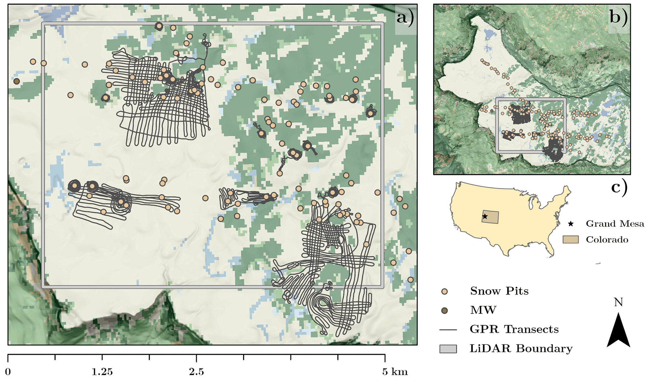
Figure 1(a) Study area map of snow pit locations (yellow circles), the Mesa West weather station (brown circle), GPR transects (black lines), and the lidar boundary (grey wireframe). Land-cover classification identifies the forested areas as green and lakes as blue. (b) Inset map of Grand Mesa, Colorado, depicting the extent of the dataset acquired during the NASA SnowEx 2020 Intensive Observation Period at Grand Mesa, Colorado (Hiemstra et al., 2021). (c) Inset map of the contiguous US which identifies the location of Grand Mesa, Colorado. Land-cover classification data were accessed from the 2016 National Land Cover Database (Dewitz, 2019). Slope hillshade data were accessed from the USGS 3D Elevation Program (Lukas and Baez, 2021). Cartographic boundary files were accessed from the Census Bureau's Master Address File/Topologically Integrated Geographic Encoding and Referencing geographic database (US Census Bureau, 2020). The geographic coordinate projection of these maps is UTM zone 12 N; EPSG code 32612.
Ground-penetrating radar records the amplitude and travel time of each of a series of echoes from short-pulse electromagnetic waves as an image in range-time and position coordinates. Provided the snow depth is constrained, GPR analysis can estimate the snow density, or, by exploiting a ray path function of travel time versus antenna separation (offset), the snow depth and density can be estimated independently (e.g., Griessinger et al., 2018; Meehan et al., 2021). By combining snow depths from drone-based aerial photogrammetry or lidar with GPR travel times, snow density has been estimated along 100 m scale transects and then analyzed as a time series to understand the densification process (McGrath et al., 2022; Valence et al., 2022; Bonnell et al., 2023) and explore extrapolation across the study-plot scale (Yildiz et al., 2021).
Our work leverages airborne lidar snow depths in tandem with GPR two-way travel times (TWTs) to facilitate density estimates. These data then become input to multiple ML regression approaches to develop and compare spatially continuous estimates of bulk snow density and SWE across the entire lidar domain. Sensitivity testing of regression models informed the model repeatability and forcing processes for spatial density patterns at Grand Mesa, Colorado, USA. As part of this workflow, we developed a reliable automated radar coherence approach for automatically interpreting the TWTs needed to retrieve snow density. This work highlights interactions between snow, terrain, vegetation, and wind in the densification process as well as the importance of careful ML model parameterizations and validation approaches. Our work addresses the need for high-accuracy distributed density measurements as assimilation data for parameterizations of snow densification to reduce runoff model uncertainty. Additional knowledge of the spatial patterns and predictors of density may improve the calibration, validation, and parameterization of radar remote-sensing SWE retrievals.
2.1 Study area
Grand Mesa, Colorado, is a high-elevation subalpine plateau with an average elevation of ∼ 3200 m and an area of ∼ 1300 km2. Grand Mesa has a cold and dry continental snow climate, low relief, and vegetation cover that varies from shrub steppe and subalpine meadow to dense conifer forest. These factors, along with the proximity to a regional airport, make Grand Mesa a near-ideal study area for evaluating airborne snow remote-sensing techniques and developing many challenging snow remote-sensing advancements (e.g., Boyd et al., 2022; Singh et al., 2023).
The Grand Mesa NASA SnowEx Intensive Observation Period (IOP) spanned 27 January–12 February 2020. During that time, more than 150 snow pits were excavated and nearly 38 000 in situ snow depth measurements were collected. Snow pits were distributed within forested and open areas along the swaths of the airborne remote-sensing campaign flight lines (Fig. 1).
As part of the SnowEx campaigns at Grand Mesa, five meteorological stations were installed between 2016 and 2017 and operated through the 2021 water year (Houser et al., 2022). Of these sites, the 3 m elevation wind speed and direction data measured at Mesa Middle (MM) and Mesa West (MW) were examined as the validation for snow transport potential and to quantify differences in exposed and sheltered terrain (Appendix C1). The MW station was in exposed western terrain of the mesa, 350 m west of the study domain boundary (Fig. 1). The MM station is sheltered within a dense stand of conifer trees 18.7 km east of the study domain boundary.
2.2 GPR data acquisition
Two GPR instruments were operated during the first week of the Grand Mesa IOP. To acquire data within forested areas of central Grand Mesa, a conventional L-band GPR was pulled by ski during 30 January to 1 February and on 5 February (Webb, 2021). This unit was equipped with a global positioning system (GPS) receiver with 2.5 m horizontal accuracy. In open areas, we deployed a multi-polarization L-band GPR fastened within a sled that was pulled by a snowmobile at approximately 3 m s−1 in the open areas of the central and south regions of western Grand Mesa on 28 and 29 January and 4 February 2020 (Meehan, 2021). The snowmobile was driven along the edges of forested stands but could not travel through densely treed areas. The multichannel L-band GPR was configured with one transmitting antenna and two receiving antennas that were oriented parallel (H) and orthogonal (V) to the transmitter (H). The transmit and receive antennas were separated by 25 cm. Using this GPR configuration, we simultaneously acquired the radar imagery in co- and cross-polarizations (HH and HV). A global navigation satellite system (GNSS) receiver with approximately 1 m horizontal position uncertainty was located on the snowmobile 5 m away from the GPR array. We applied a geometric correction to relocate the coordinate positions to the antenna midpoint of each channel. The GPR data were acquired within a few meters of, but not directly beside, the snow pit walls, which necessitated a radius for pairing retrieved or modeled data with validation observations. The GPR systems were operated continuously, collecting approximately 30 traces per second, given the duration of the time window for each trace (30 ns), the sample interval (0.1 ns), and the number of stacks acquired (2). Due to differences in the travel speed, the spatial interval of the GPR traces collected via snowmobile is approximately 10 ± 1 cm, while the interval for traces collected by ski is 5 ± 1 cm. We used piecewise cubic Hermite interpolating polynomials (Kahaner et al., 1989) to fix a geolocation to every acquired trace, as the GPS acquisition rate was 1 Hz. Throughout this week, we acquired 144 km of quasi-gridded and spiraled snowmobile-driven radar transects and 16 km of skied spiral transects in the forest. Spiral transects were coincident with depth measurements. We used a 4.5 km by 3.5 km portion of the snow-on lidar acquisition to bound the GPR transects (Fig. 1) and omitted any transects acquired beyond the lidar boundary.
2.3 GPR data processing
Multi-polarization radargrams were processed using an automated routine (Meehan, 2024). We applied a frequency–wavenumber (F-K) filter as a 2D bandpass filter (Kim et al., 2007). Time-zero correction was performed automatically using the modified energy ratio first-break picker (Wong et al., 2009). We removed coherent noise by subtracting the median trace from the radargrams (Kim et al., 2007). The trace amplitudes were corrected for spherical divergence by applying t-squared scaling as a signal gain function (Yilmaz, 2001). In a random-noise removal step, we then applied edge-preserving smoothing (Kuwahara et al., 1976). This routine emphasized the continuity and amplitude of the ground reflection, which benefited the method for automatically picking the travel times. The GPR data within forests were processed with a bandpass filter, time-zero correction, and background subtraction prior to manual interpretation using a semiautomatic algorithm and are available through the National Snow and Ice Data Center (Webb, 2021). The slower-paced data acquisition by ski improves the quality of the radargram, which benefits the tracking of the ground surface in the more variable forest environment.
2.3.1 Multi-polarization coherence for automatic two-way travel-time determination
The rough ground depolarized the L-band radar signal, and thus we used the coherence between the co- and cross-polarized channels as a filter that illuminates the ground reflections and removes the planar reflections of the snow stratigraphy. We paired the co- and cross-polarization radargrams into shot gathers, which are the bins of traces that share the same transmitter location. The automatic travel-time pick is determined by maximizing the coherence between the co- and cross-polarization shot gathers. To measure the coherence for each pair of traces, we applied the unnormalized cross-correlation sum:
which is half of the summed difference between the energy of the stacked traces and the energy of the input traces (Neidell and Taner, 1971). The calculation in Eq. (1) is performed in a sliding window over N=11 samples, which is evaluated at every sample (j) of the GPR signal (Si,j) for channel i (M=2). The HH–HV coherence (CHH-HV) at each shot location is then normalized by the maximum coherence,
Small (one-wavelength) offsets introduce waves that have an approximately normal incidence with respect to the reflection horizons, such that the nonlinear effects of travel-time moveout are negligible and snow depth can be directly retrieved from the measurement of TWT. Because the offsets are equal, the travel times to the ground for each channel are equal to within a small error (due to the variability of the ground surface inside the radar footprint), and therefore the two channels sum coherently.
We automatically chose the travel time with the maximum coherence of each trace and subtracted 1 ns ( wavelet) to estimate the first break of the reflection (Booth et al., 2010). We then applied a median filter to remove outliers and reviewed the automatic picks for any systematic errors.
2.4 Observed, derived, and explanatory data
2.4.1 In situ measurements
Snow pit observations and manual depth probe measurements were collected throughout the 27 January to 12 February 2020 IOP to serve as a validation for the SWE and snow depth retrieved by airborne remote sensing. Snow pits were measured for the snow depth, density, water equivalent, temperature, wetness, liquid-water content, grain size, and stratigraphy (Vuyovich et al., 2021). Snow density (ρs,pit) was measured continuously every 10 cm from the snow surface to the ground using a 1000 cm3 wedge sampler, with duplicate samples. If the difference between the two measurements at a given depth exceeded 10 %, the density was sampled a third time, and bulk density was then calculated by averaging all the measurements for each snow pit. Because the density snapshot we retrieved is valid for the time of the lidar flight, we corrected the measured density to 12:00 on 1 February using densification rates determined by linear regression for both open and forested areas. Liquid-water content was estimated by combining the density and in situ measurements of dielectric permittivity in an empirical formula, which showed that the snowpack remained almost completely dry throughout the IOP (Webb et al., 2021). Snow depth measurements (hs,probe) were collected using geolocated probes (± 3 m spatial accuracy) along spiral transects (∼ 60 m radius) centered around pits (Hiemstra et al., 2020).
2.4.2 Lidar snow depth
Snow depth (Hs,lidar) was estimated from repeated airborne-lidar point cloud surface elevations of snow-free and snow-covered terrain (e.g., Lague et al., 2013). The Airborne Snow Observatories (ASOs) performed the snow-free acquisition on 26 September 2016 (Painter et al., 2016; Painter and Bormann, 2020) and NV5 Geospatial (formerly Quantum Spatial Inc.) acquired snow-covered surface elevations during the IOP; both had a point density of approximately 20 points m−2. We selected the 1–2 February 2020 flight to minimize temporal differences with the GPR and resulting errors due to snow redistribution and densification. We transformed the 2016 snow-free vertical datum into NAVD88/Geoid 12B (the same as the 2020 snow-on) using NOAA VDatum 4.3 software (NOAA, 2021). Then, we applied the point-cloud-differencing method to estimate snow depth on a 1 m grid (Appendix B1). Negative snow depth values were filtered as no-data values. After computing the snow depth, the 3 m ASO bare-earth and vegetation data products were resampled using the nearest-neighbor approximation to the 1 m resolution of the snow-covered SnowEx 2020 lidar acquisitions, and the coordinate system was transformed from UTM zone 13 N to UTM zone 12 N. As a comparison between our lidar snow depths and data processed using raster differencing, we used the 1–2 February 2020 ASO-acquired snow depths and upscaled Hs,lidar to 3 m using the nearest-neighbor method.
2.4.3 Lidar–GPR-estimated density
We combined the lidar snow depths with the GPR TWTs to calculate the radar wave velocity, which is only a function of density in dry snow. We applied a k-d tree searcher (Bentley, 1975) to find the lidar coordinates within a 1 m radius of the GPR TWTs. We then used the median values of the TWTs within a 1 m radius of these coordinates to interpolate to the lidar grid.
The average electromagnetic wave speed in the snowpack was estimated using
for each of the coincident lidar snow depths (Hs,lidar) and GPR two-way travel-times (τ). We then related the electromagnetic wave speed to the dry snow density using the Complex Refractive Index Method (CRIM; Wharton et al., 1980):
The CRIM equation relies on the known wave speeds of the pore space (va = 0.3 m s−1) and ice matrix (vi = 0.169 m ns−1), the measured bulk wave speed of the snowpack (vs,lidar-GPR; Eq. 3), and the density of ice (ρi = 917 kg m−3) to determine the dry snow density (ρs,lidar-GPR; Eq. 4).
2.4.4 Wind and terrain exposure
Wind data were examined from 1 October 2019 through the end of the SnowEx IOP on 12 February 2020. Hourly air temperature data parameterized an empirical relationship to determine the threshold for snow-transportable wind speed (Li and Pomeroy, 1997). For values exceeding this threshold minus the 95 % confidence interval, we then determined the median wind speed and direction for snow transport (Fig. S4b). We utilized the maximum upwind slope (Sx) and wind factor (Winstral et al., 2002; Appendix C1) as parameters explaining the patterns and processes captured by the ML regression ensemble, rather than incorporating this information as model predictors of snow density. To validate the GPR–lidar-estimated training data and the modeled results, we calculated the correlation between the model input and output and the Sx and wind factor rasters for all wind directions.
2.5 Spatial scales of variability for snow depth, travel time, density, and SWE
We examined the differences in snow properties between forested and open areas using generalized relative semi-variograms (Isaaks and Srivastava, 1989). The generalized relative semi-variogram describes the average percent variability, relative to the mean, as a function of separation distance between observations. To estimate the spatial variability of the snow depth, TWT, density, and the resulting SWE of the 1 m gridded data along the radar transects, the experimental variograms were first calculated in 1 m bins up to a 250 m lag and then fitted with exponential models via least squares to estimate the range, sill, and nugget parameters (e.g., Cressie, 1985). We used an exponential variogram model for which the correlation length is equal to 3 times the range parameter. We created 250 realizations of the experimental variogram calculation using Monte Carlo simulation with 10 % random subsampling to assess the means and standard deviations of the variogram parameters (Efron and Tibshirani, 1986).
2.6 Modeling of the spatial snow density
2.6.1 Machine-learning model ensemble
To distribute the spatial observations of average snow density to areas without GPR observations, we tested three regression techniques: multiple linear regression (MLR; Andrews, 1974; Appendix A1.1), random-forest regression (RF; Breiman, 2001; Appendix A1.2), and artificial-neural-network regression (ANN; Jain et al., 1996; Appendix A1.2). We examined the ∼ 16 km2 area of the lidar domain, which closely bounded the extent of the GPR survey. A set of normalized predictor variables, notated with capital lettering, were developed using the elevations of four lidar rasters (the bare-earth elevation (Zg), snow-covered elevation (Zs), snow depth (Hs), and vegetation height (Hveg)); the aspect, slope, and x and y derivatives of the elevation rasters (excluding Hveg); and the distance to the nearest vegetation ≥ 0.5 m (Sveg). Aspect rasters were transformed by the cosine to remove the wrapping ambiguity around north. We smoothed the elevation, vegetation height, and snow depth rasters using a median filter with a 5 m × 5 m window and the derivatives of these rasters (slope, aspect, dx, and dy) with a 25 m × 25 m window. Regression models were trained on the lidar–GPR-estimated snow density using cross-validation and were applied to the surrounding terrain. By retraining the model architectures on random subsets of data, 50 model ensembles were generated and then averaged for both RF and ANN regressions. The model hyperparameters were developed such that the variance of the predictions in pixels where training data exists matches that of the predictions. The appropriate hyperparameterization coincided with an R2 of approximately 0.8. An ML snow density ensemble () was composed by averaging the MLR, RF, and ANN outputs. For more detail on the model hyperparameterization and predictor importance, see Appendix A.
2.6.2 Gaussian random field model
To serve as a baseline for model assessment, a Gaussian random field snow density model was synthesized from the statistics of the in situ density measurements and the correlation length of snow density estimated via variogram analysis. Provided that the empirical variogram function was available, a covariance matrix was determined between all pairs of points in the ∼ 16 km2 domain. Using Cholesky decomposition, the large covariance matrix was efficiently inverted to determine a matrix of weights with the desired covariance properties (Vecherin et al., 2022). The synthetic snow density model was then generated by multiplying a normal random vector with zero mean and the same standard deviation as the in situ observations by the weighting matrix and adding the mean value of the density observations.
2.7 Distributed snow water equivalent and uncertainty
Multiplying Hs,lidar by yielded SWE () distributed throughout the lidar domain. As a benchmark example drawn from in situ sampling, we also distributed SWE using the average snow density (276 kg m−3), the average density of both open (280 kg m−3) and forest (257 kg m−3) areas, and the Gaussian random field model (bs,lidar-Rand). See Appendix B3 for additional details. We upscaled to 50 m resolution using the nearest-neighbor approximation for comparison with the 50 m ASO SWE.
Using simple linear regression, we modeled the snow density errors for . No correlation between error and snow depth was found, and the RMSE (11 cm) was used to estimate the random error. Using the random errors in snow depth, linear errors in density, and linear error propagation, we estimated the uncertainty in to first order (Raleigh and Small, 2017). Appendix B4 has further information on SWE uncertainties regarding sampling errors estimated from in situ measurements.
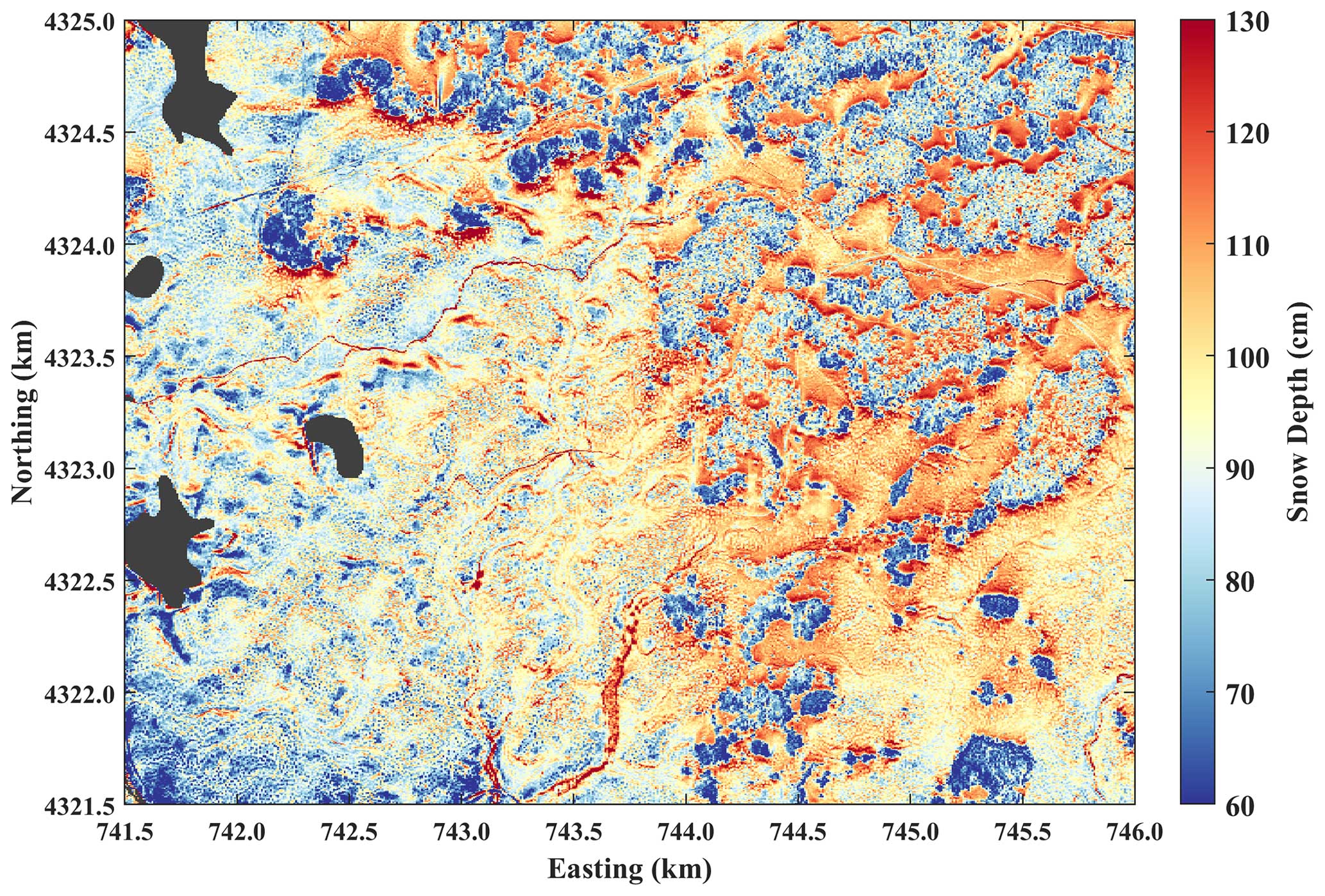
Figure 2Snow depths (1 m resolution) from the 1 February 2020 lidar flight. The western half of the domain is relatively unforested shrub steppe (lakes are masked in black), while the eastern half has stands of dense forest (see Fig. 1). The color map is centered on the mean value.
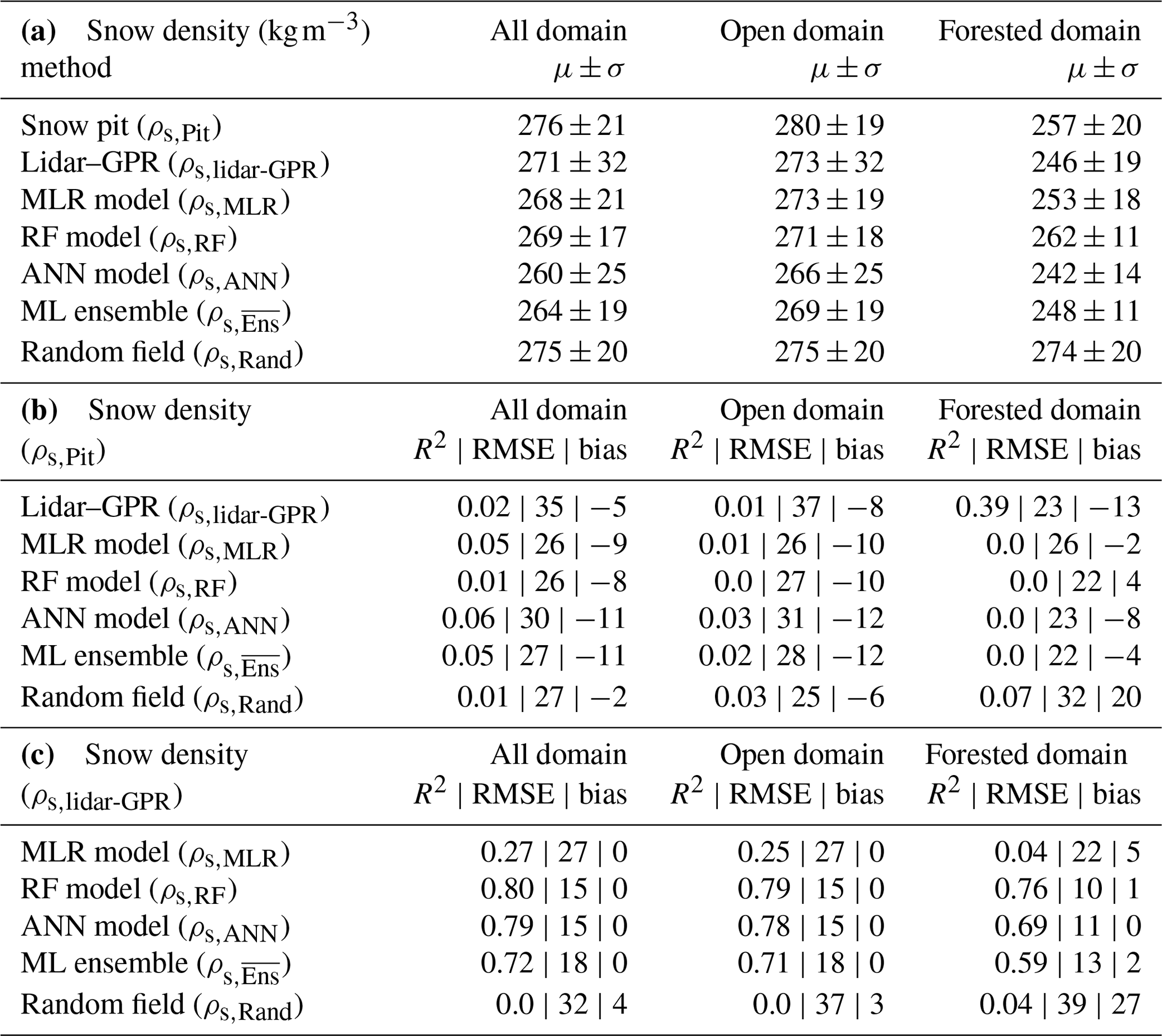
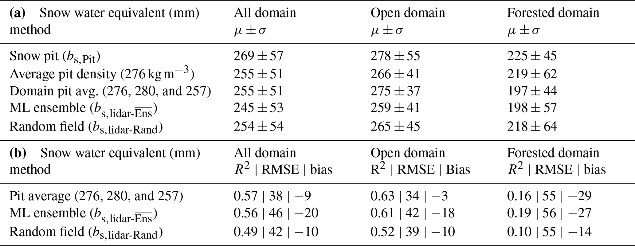
Table 1(a) Mean and standard deviation values of the snow-pit and probe-measured snow depths. (b) Estimates co-located by the lidar and GPR techniques and gathered from within a 1 m radius of the in situ observations are compared to the in situ observations.
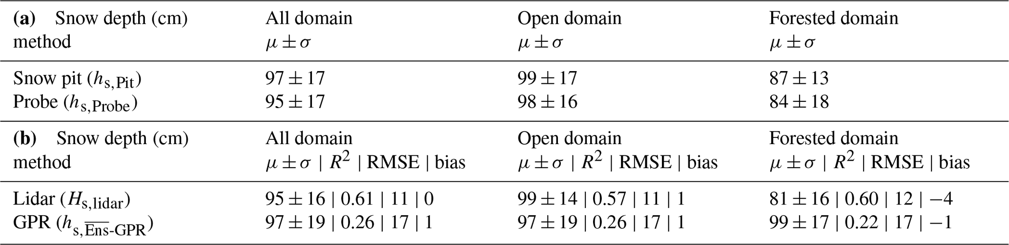
3.1 Snow depth
The lidar-derived snow depths show an overall increasing trend from west to east in addition to smaller-scale patterns near vegetation, with deeper snow around the perimeter of treed areas and shallow snow on the ground beneath tree canopies (Fig. 2). This pattern is consistent with previous snow depth distribution studies of Grand Mesa (e.g., McGrath et al., 2019). The mean lidar snow depth for the entire domain is 92 cm with a standard deviation of 18 cm. In open areas (Hveg < 0.5 m), the mean lidar snow depth is 96 ± 15 cm, while in the forest (Hveg ≥ 0.5 m), the mean lidar snow depth is 79 ± 23 cm. In validation snow depth observations (hs,Pit and hs,Probe), the average snow depth over the lidar domain is 95 ± 16 cm (R2 = 0.61, RMSE = 11 cm, ME = 0 cm). Lidar- and GPR-estimated snow depths within the open domain and those within the forested domain are also compared to in situ snow depths (Table 1). In snow depth comparisons between Hs,lidar, Hs,ASO, and Hs,Probe, the two lidar processing methods showed similar correlations (R2 ≈ 0.6) and root-mean-square errors (RMSE ≈ 12 cm). However, Hs,ASO (86 ± 16 cm) underestimates snow depth by 7 cm, while Hs,lidar (93 ± 16 cm) is unbiased on average (Fig. S1 and Table S1 in the Supplement).
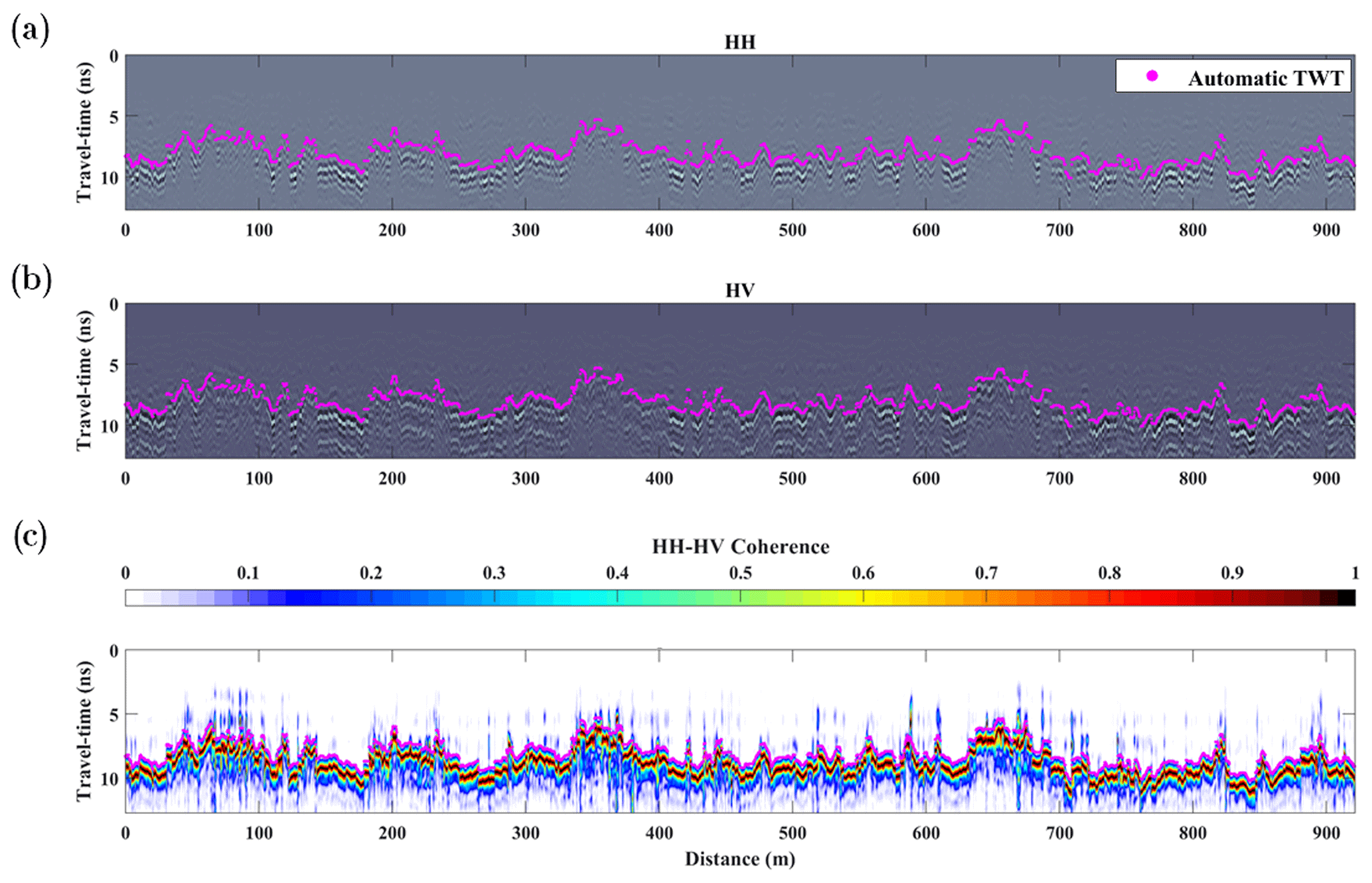
Figure 3A 900 m GPR transect with autopicks in magenta for (a) HH and (b) HV profiles of travel time and (c) the coherence of these radargrams (Eqs. 1 and 2).
3.2 GPR travel time
Ground-penetrating radar travel-time data analyzed at crossover locations exhibited a root-mean-square deviation of 1 ns with a bias of 0 ns, and no systematic bias between the two GPR instruments was found. Approximately 90 % of the travel-time data applied in this work were automatically determined using the coherence method, where less than 1 % of the automatic picks required manual correction. To illustrate this, automated picks are overlaid on the radargrams of a 900 m long transect in Fig. 3. The resulting TWT data produced from this method and used in this study are available through the National Snow and Ice Data Center (Meehan, 2021).
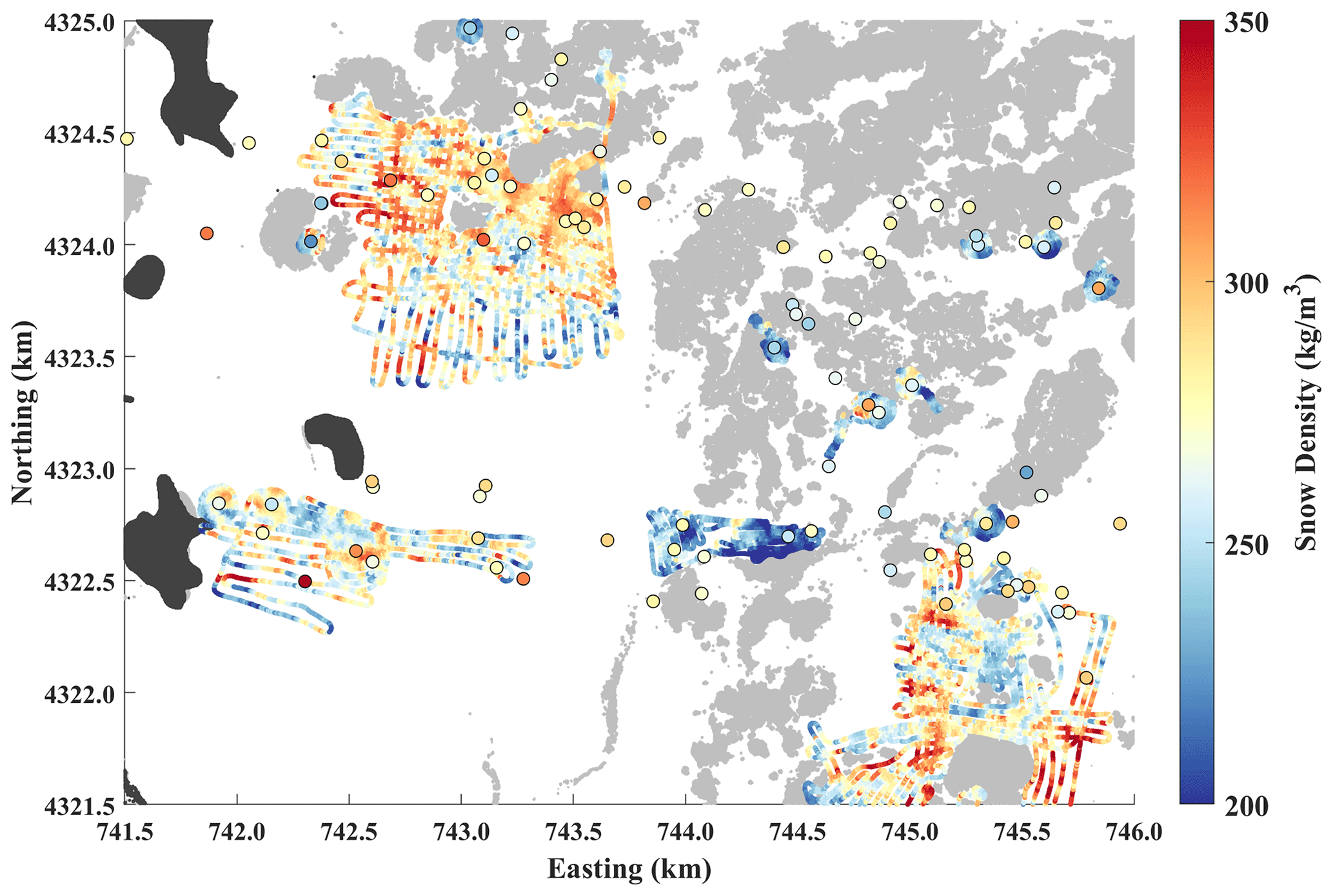
Figure 4Bulk snow density along radar profiles, estimated by combining lidar snow depths with GPR TWTs. Average densities measured in the 96 snow pits within the lidar boundary are overlaid as larger makers. Forested areas (grey) and lakes (black) are shown. The color map is centered on the mean value.
Table 2(a) Mean and standard deviation for snow pit, lidar–GPR (Sects. 2.4.1 and 2.4.3), and modeled densities. Snow pit means and standard deviations are estimated from all available data (N = 96 snow pits for the entire domain, N = 79 for the open domain, and N = 17 for the forested domain). (b) Comparison between snow pit densities and estimated densities. Statistics (R2, RMSE, and bias) are measured from a subset of snow pits within 12.5 m of the GPR transects (N = 42 for all the domain, N = 36 for the open domain, and N = 6 for the forested domain). (c) ρs,lidar-GPR-estimated densities are evaluated against modeled results.
3.3 Lidar–GPR-estimated density
The lidar–GPR-retrieved average snow density shows repeatable structure at the many crossover locations and greater variability in the open terrain than areas sheltered by forest canopies (Fig. 4). The integrated lidar and GPR data resolve lower spatial frequency patterns than the snow pit observations, which are sparse and have limited spatial support. When compared to snow pit observations, the relative RMSE among the 37 snow pits that are within 12.5 m of the GPR transects is 35 kg m−3 or 13 % (Table 2). The ρs,Pit and ρs,lidar-GPR data are both normally distributed, as evidenced by a Z test (Appendix B3) with overlapping standard deviations. The maximum upwind slope and wind factor evaluated on GPR transects show the strongest correlation (R = −0.45 and R = 0.48, respectively) in the 225 and 220° directions (Fig. S2 and Table S2).
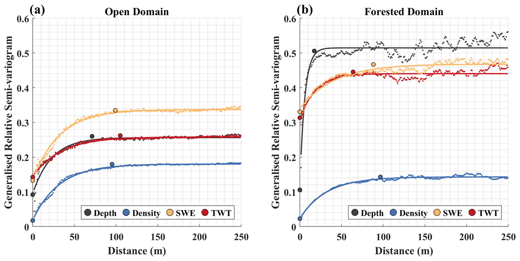
Figure 5Generalized relative semi-variograms in (a) open and (b) forested areas for lidar snow depth, GPR TWT, average density retrieved along the GPR transects, and the resulting SWE. Experimental variograms were fitted with an exponential model to determine the variogram parameters. The larger markers represent the average nugget, sill, and correlation length estimated by Monte Carlo subsampling.
3.4 Spatial variability of the lidar snow depth, GPR travel time, density, and SWE
The generalized relative semi-variogram allows us to examine the differences in the length scales of variability among depth, density, SWE, and TWT within the forested and open areas of Grand Mesa (Fig. 5). Table S3 overviews the generalized relative semi-variogram parameter estimates (nugget, sill, and correlation length). TWT and SWE consistently exhibited similar correlation lengths (∼ 100 m) and nugget variability within the forested (∼ 35 %) and open (∼ 15 %) areas. Snow depth and TWT reached comparable maximum variabilities in open areas (∼ 25 %). Depth variability in the forested areas (∼ 50 %) was greater than that of TWT and SWE (∼ 45 %). The median distance between snow pits is ∼ 150 m, which indicates that average snow pit observations are independent of each other and unable to resolve spatial patterns at a finer scale.
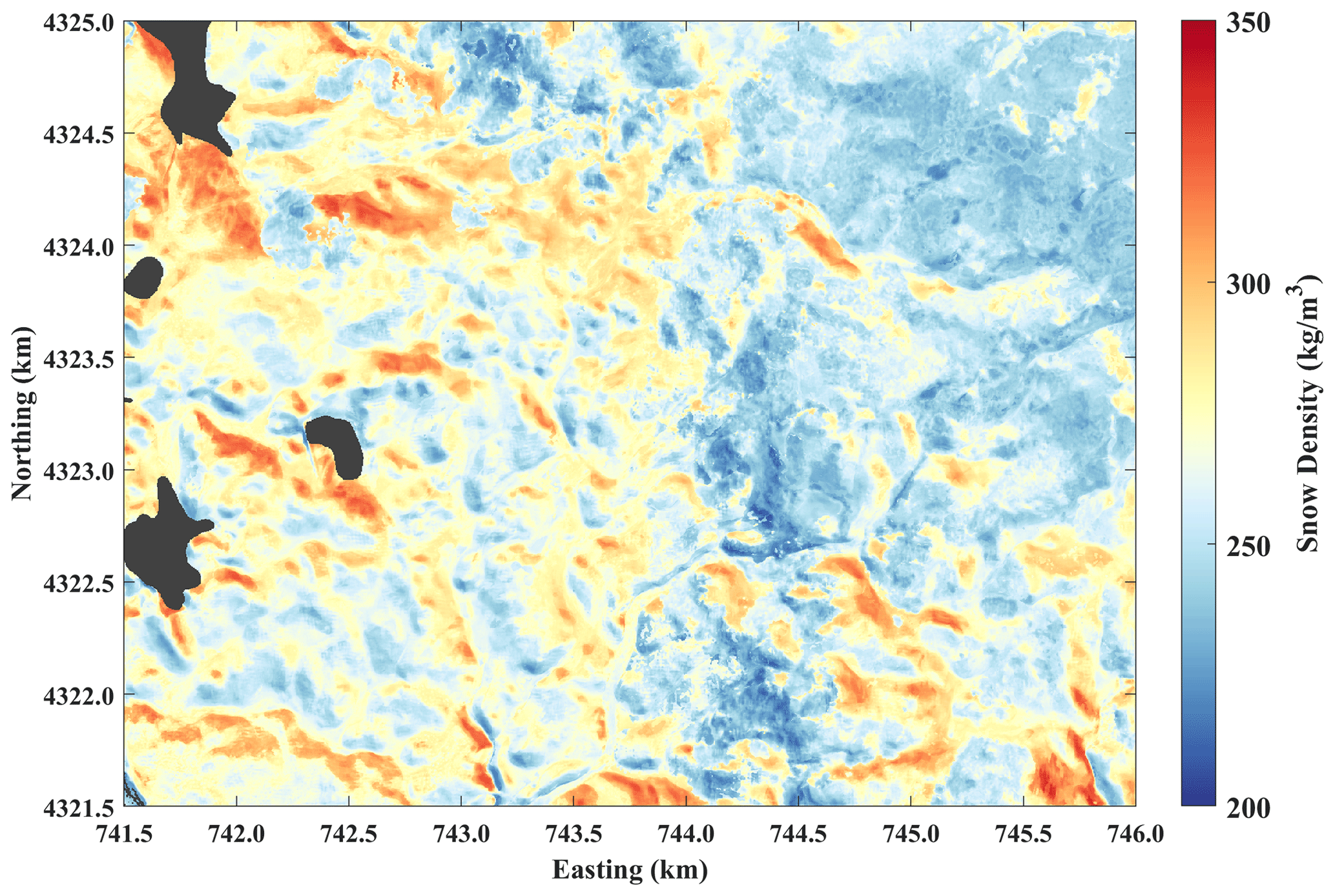
Figure 6Snow density distributed spatially using the ML regression ensemble average (). The color map is centered on the mean value.
3.5 Density modeled using machine-learning regression and a Gaussian random field
Using supervised ML regression, three models were generated from lidar information (Fig. S3a–c). Using prior information from the in situ snow pit observations a randomly distributed density was synthesized (Fig. S3d). The mean of the regression-based ensemble was taken to generate (Fig. 6). Generally, the regression models predict higher snow density in the open and exposed areas than in areas that are protected from the wind by trees. Each of these five models are evaluated against ρs,lidar-GPR and ρs,Pit (Table 2). The ML regression snow densities are generally uncorrelated (R2 ≈ 0.05) and have an RMSE of ∼ 10 % with snow pit observations. The spatial similarity of these models is presented in Appendix A3.
3.6 Model representation of wind, terrain, and vegetation effects
Maximized correlations between the terrain exposure parameters for all wind directions and the ML regression modeled snow density agree with the median wind direction that is able to transport snow (6.4 m s−1 at 200°; Fig. S2). The wind speed and direction data from the Mesa West meteorological station (Houser et al., 2022) are presented for all of the time period from 1 October to 12 February (Fig. S4a) and the time period where the wind was strong enough to transport snow (Fig. S4b). Upwind-slope and wind-factor parameters calculated for a 200° wind direction are provided for reference (Fig. S5). No correlation was evident between these wind exposure parameters and the Gaussian-random-field-distributed snow densities (Table S2).
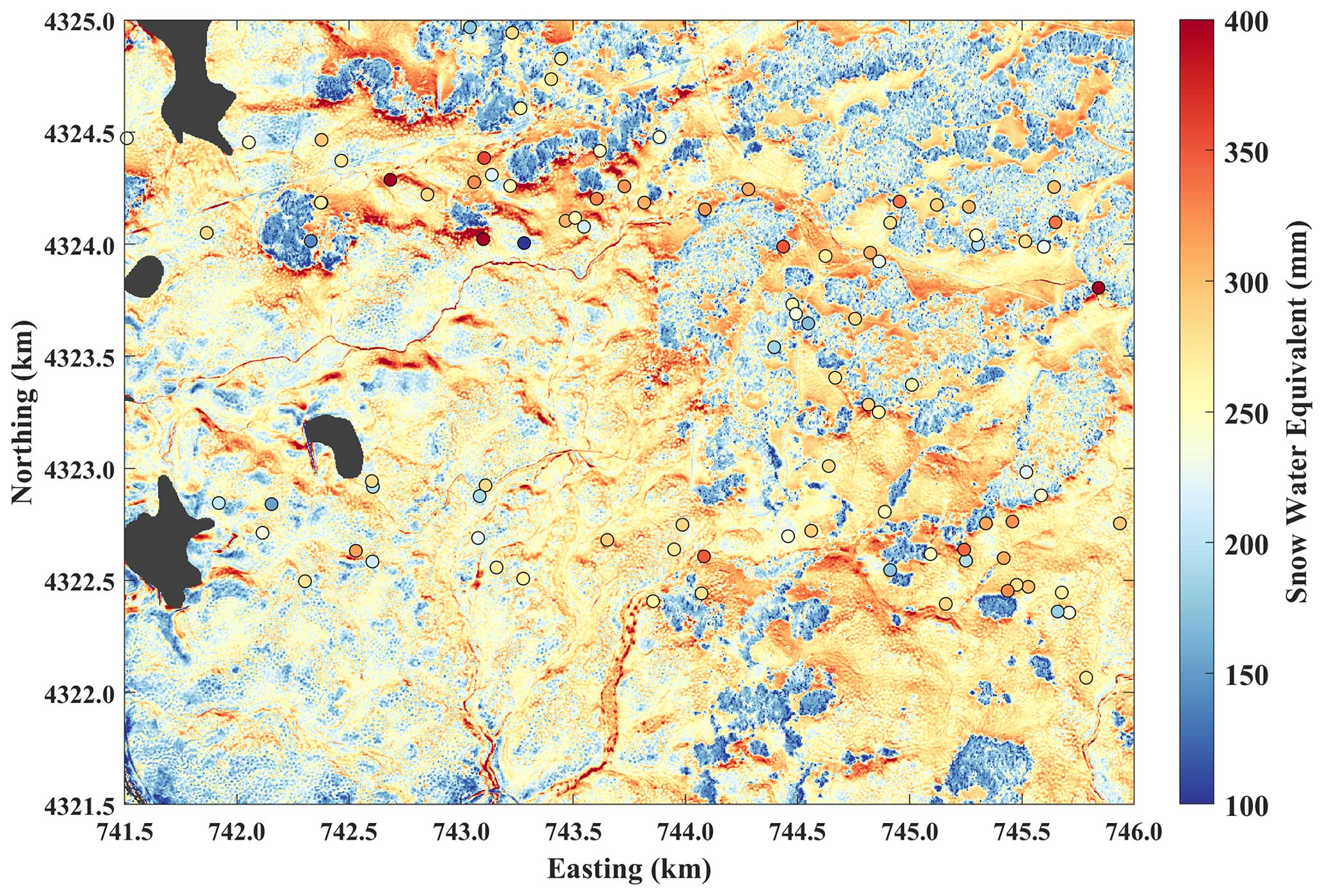
Figure 7Spatially distributed snow water equivalent estimated using the regression ensemble mean density () and lidar snow depths (Hs,lidar). Forests and wind-scoured areas tend to have lower SWEs, and forest perimeters have higher SWEs. The meter-scale stippled texture is the result of low-stature vegetation (Hveg < 0.5) and boulders, which both reduce the snow depth and decrease the snow density. Large markers are SWE values measured at snow pits. Lakes are masked in black. The color map is centered on the mean value.
Table 3(a) Mean and standard deviation values of the snow water equivalent measured in snow pits and distributed by lidar snow depths using an average snow pit density value (276 kg m−3), the average snow pit density in each respective domain (276, 280, 257 kg m−3), the regression ensemble densities, and the random-field densities. In situ means and standard deviations are estimated from all available data (N = 96 snow pits for the entire domain, N = 79 for the open domain, and N = 17 for the forested domain). (b) Comparison of SWE between snow pit observations and distributed estimates obtained by multiplying lidar snow depths by the average density measured from snow pits in the respective domain, the ML-ensemble-modeled densities, and the random-field-synthesized densities.
3.7 Spatially distributed snow water equivalent
SWE distributed within the ∼ 16 km2 domain (Fig. 7) underestimated the snow pit average SWE by 20 mm (R2 = 0.57; RMSE = 46 mm; Table 3; Fig. S6a–c). Upscaling to 50 m resolution resulted in decorrelation (R2 = 0.03) and increased error (RMSE = 60 mm), and the bias remained nearly the same (−18 mm; Fig. S6d–f). ASO SWE (bs,ASO; 50 m resolution) had similar errors (RMSE = 57 mm) and bias (−21 mm) and a low correlation (R2 = 0.1) to measurements (Fig. S6g–i). The 50 m had a mean SWE and standard deviation of 245 ± 33 mm, while bs,ASO was 236 ± 45. The average snow density of bs,ASO was 274 kg m−3 (versus a value of 264 kg m−3 for ). Distributing SWE using the average measured value led to a lower bias (−9 mm) and root-mean-square error (38 mm) than . Using a constant density causes the SWE spatial patterns and data correlation to be driven solely by snow depth. Tested against the Gaussian-random-distributed density (R2 = 0.49), the ML-regression-modeled densities explained more variation in the distributed SWE estimates (R2 = 0.56) – about as much as snow depth alone. For comparison, is presented alongside Hs,lidar and in Fig. S7.
3.8 Contributions of uncertainty
3.8.1 Lidar snow depth
Hs,lidar snow depths were computed from point cloud differencing rather than raster differencing. The relative accuracy of the snow depth measurement was estimated at 7 cm (based on the maximum standard deviation of the point cloud differencing method), which agrees well with previous lidar error assessments using this approach (Hojatimalekshah et al., 2021). The absolute accuracy of the snow depths (11 cm) was determined by comparison to validation snow depth measurements, which shows 0 cm of bias on average over all measurements (Table 1). On plowed roads, we observed snow depths ranging between 0 and 5 cm (Fig. S8).
3.8.2 Lidar–GPR co-registration
We estimated the horizontal accuracy of the multi-polarization GPR positions, which had a clear-sky view and a GNSS receiver, at ± 1 m. The GPR system operated within the forest stands had lower GPS fidelity, which we conservatively estimate at ± 3 m. Ground validation showed less than 1 cm horizontal position uncertainty within the lidar point cloud. We found that errors in the co-registration of the lidar and GPR data are the leading source of error in the estimated densities. The overall accuracy of the spatial registration between the lidar and GPR varies on the order of a few meters.
Sensitivity analysis showed how measurement errors propagate into the lidar–GPR-measured snow density (Appendix B2). At the 1σ confidence interval, we found that measurement errors are on the order of 10 cm for lidar and 1 ns for GPR, which may translate into errors in the density estimate of 150 kg m−3 or greater. Variogram analyses show that beyond 10 m, these errors are spatially uncorrelated and can be treated with random noise filtering. After median filtering and interpolating through outliers, error estimates reduced to 30 kg m−3 (Appendix B2).
3.8.3 Spatial and temporal support of density measurements
Measurements accumulated over 12.5 m distance introduce inherent variability on the order of 10 % (Sect. 3.4). We found that the expected variability among co-located ρs,lidar-GPR is approximately 2 %, which is consistent with replicated in situ density observations (ρs,Pit). The average density sampled from each of the snow pit columns (within 1 m) shows high repeatability, with a root-mean-square deviation of 2.5 %. We observed linear temporal trends in snow densification of 0.07 in forested areas and 0.13 in open areas. These trends were removed and were not considered within uncertainty analyses.
3.8.4 SWE uncertainty
The errors between Hs,lidar and hs,Probe are uncorrelated when compared to Hs,lidar (R2 = 0.04). However, the errors between and ρs,Pit are negatively correlated against (R2 = 0.35, RMSE = 27 kg m−3). The errors in snow depth and density are uncorrelated (R2 = 0.03), with negligible covariance (Fig. S9). The distributed relative SWE uncertainty is presented in Fig. S10 and is negatively correlated with the distributed SWE (R2 = 0.57). The distributed absolute SWE uncertainty (Fig. S11) is weakly positively correlated with (R2 = 0.22). The median SWE uncertainty is 13 % (30 mm), which breaks down into 15 % (29 mm) median uncertainty in the forest and 13 % (31 mm) median SWE uncertainty in the open areas. The relative uncertainty is greater within forests due to the decreased total SWE within stands. Median snow density relative uncertainty is 4 % (10 kg m−3). Median snow depth relative uncertainty is 12 % (11 cm). Median lidar snow depth relative uncertainty is 12 % (11 cm) in open areas, while in the forested areas median depth uncertainty is 14 % (13 cm). Median snow density uncertainty is 4 % in both open and forested areas, with more extreme density values having greater uncertainty due to linear error modeling. Had snow density been modeled as a random variable, the density would contribute an error of 10 % (27 kg m−3), equating to 16 % uncertainty in SWE on average.
4.1 Multi-polarization GPR
This work advances the utility of GPR for seasonal snow applications by resolving the spatial snow density and SWE through the integration of remotely sensed lidar and GPR observations. Grand Mesa is a good site for testing our approach of combining lidar and GPR for density and SWE retrieval, yet it presents many challenges for GPR analysis because of the abrupt discontinuities along reflection horizons due to vegetation and boulders on the ground surface. By exploring the effects of depolarization on L-band GPR signals, we developed a new, automated GPR processing workflow that reliably identifies the ground surface beneath the snow cover. This advance encourages the collection of large multi-polarization GPR datasets for operational use by removing the subjectivity involved in the GPR post-processing and interpretation and alleviating the labor of manually interpreting radargrams through an objective function.
4.2 SWE uncertainty
Our work characterized the measurement uncertainties and the resulting SWE uncertainty in pursuit of the goal of 10 % uncertainty in global SWE estimation (National Academies of Sciences, Engineering, and Medicine, 2018). We found that GPR TWT and lidar snow depth contribute approximately equal uncertainties to the retrieved snow density. The uncertainty in lidar snow depth tends to vary spatially and is dependent on landscape characteristics such as slope and vegetation (Deems et al., 2013). However, our evaluation of snow depth in forested and open areas did not suggest that lidar snow depth errors were greater beneath the tree canopy (Table 1). The relative SWE uncertainty resembles the snow depth distribution, with shallow snow within forest stands yielding greater relative uncertainty. The absolute SWE uncertainty resembles the snow density patterns, especially in areas of anomalous snow density, where the modeled errors are greatest. Our uncertainty analysis (Fig. S10) suggests that, even when using innovatory measurements from airborne and ground-based sensors, 10 % uncertainty is difficult to achieve. However, the joint lidar–GPR technique shows promise for SWE remote-sensing calibration and validation and demonstrates advantages over contemporary SWE retrievals at plot to forest-stand scales.
4.3 Geolocation errors in sensor fusion
Though the signals from lidar and GPR instruments are repeatable and coherent, the leading source of error in our density measurement is spatial misalignments (potentially sourced from geolocation inaccuracies, point cloud to raster processing, and coordinate transformations) that are on the scale of the 1 m resolution data products. In some locations, the co-registration between the two instruments may be nearly exact, and the resulting error will be low. We found by cross-correlating the GPR and co-located lidar snow depth transects that misalignments of approximately 1–5 m are possible. Utilizing 3 m resolution lidar snow depths paired with GPR TWTs for snow density retrieval did not reduce the errors. To evaluate how spatial misalignments impact the training data, the predictor data, and the regression model output, and to estimate the uncertainties introduced upon integrating the cross-platform sensor data, we created multiple sets of training data by effectively perturbing where lidar–GPR transects are aligned via cross-correlation lagging and introducing common practice mistakes in the sensor integration, such as mixing the geographic coordinate system of the data between NAD83 and WGS84. We found that perturbing the sensor integration introduces less than 1 kg m−3 error into the modeled density on average (up to 5 kg m−3 in forest stands), that outlier filtering is robust to sensor integration errors, and that this error is small relative to the overall SWE uncertainty.
4.4 Spatial variability in snow hydrological properties
Measurements retrieved from GPR profiles permitted us to quantify the spatial length scales of variability in TWT, snow depth, snow density, and SWE. We determined that density measurements up to ∼ 100 m apart are correlated. These findings differ from a previous variogram analysis that found correlation lengths for snow density of less than 10 m at a smaller study site which limited the maximum lag separation to approximately 50 m (Yildiz et al., 2021). Variability is study-site dependent (Bonnell et al., 2023), and it may be that we have identified an additional longer, lower spatial frequency scaling of snow density. As it is a corollary to SWE, the two-way travel time in dry snow depends on both snow depth and density. We found that TWT and SWE consistently exhibited similar correlation lengths (∼ 100 m) and nugget variabilities in the forested (∼ 35 %) and open (∼ 15 %) areas. This finding supports TWT as an informer of spatial SWE variability. We found that snow depth and TWT reached comparable maximum variabilities in open areas (∼ 25 %), while depth variability in the forested areas (∼ 50 %) was greater than that of TWT and SWE (∼ 45 %).
In situ snow density observations have limited spatial support and tend to examine shorter length scales of variability than are expressed in distributed models or retrievable by remote sensing. As a random-sampling strategy was targeted for the IOP, the median distance between snow pit observations in our study is beyond the length scale of variability for snow density. The observations are therefore spatially uncorrelated. Snow density exhibited 4 % greater variability in the open areas than in the forests, indicating that wind exposure increased the variability and, conversely, shelter provided by terrain and vegetation tended to reduce the spatial density variability. The larger (roughly 10 m) spatial support of the lidar–GPR-estimated densities cannot directly sense subpixel correlation lengths and potentially missed a 0–5 m scale break that is more comparable to the spatial support of in situ density observations. Differences between representative observation scales may explain the weak correlation between the estimated density and the in situ measurements (R2 = 0.01 in open areas and R2 = 0.39 in forest stands; Table 2b). Our analysis of the correlation length of lidar snow depths generally agrees with the scale breaks identified in previous studies within forested and open areas (Deems et al., 2006; Marshall et al., 2006; Trujillo et al., 2009). We observed decreased correlation and increased error when upscaling the rasterized SWE to 50 m resolution, which suggests that evaluating the 50 m SWE with sparse point measurements may not be the most representative approach, and a greater than 20 % error can be expected due to spatial variability.
4.5 Density modeling using ML regression
The ML regression models developed from the lidar and GPR acquisitions during the SnowEx 2020 Grand Mesa IOP will likely have only weak predictive capabilities at other field sites, as they require model recalibration. The SWE predictions reported here represent a single snapshot in time of snow depth and density. The patterns in depth, density, and SWE may be characteristic for mid-winter dry-snow conditions, but other times of the year may exhibit different spatial patterns in all three (e.g., due to variable melt or liquid water during ripening). For each regression model, we identified the most important lidar features that are used to distribute density, and we found dependencies of predictor importance on model choice and architecture (Appendix A2). Vegetation height and proximity to vegetation greater than 0.5 m in height appeared prominent in the three regression models, whereas the dependence of snow density at Grand Mesa on elevation, slope, and aspect was weakened. We used a “kitchen-sink” approach to our regression modeling but found comparable accuracy in models using fewer parameters. Evaluations against snow pit density did not indicate an obvious best model choice, as so we averaged the regression models.
To capture the range of terrain features (i.e., elevation, slope, aspect, and forest attributes) that influence snow densification, one field campaign in the western US collected density measurements from 300 snow cores at 10–20 m intervals and 17 snow pits (Broxton et al., 2019). Based on these observations, bulk snow density was distributed at 1 m resolution using an ANN combined with the airborne-lidar-derived snow depth to estimate the SWE. Broxton et al. (2019) highlighted the importance of representing the broader landscape with distributed densities for estimating SWE by finding ∼ 30 % differences between the distributed estimates and observations from a nearby SNOTEL station. Elder et al. (1998) used a simpler, three-feature (net radiation, slope, and elevation, with an intercept) MLR model that was trained on density observations of five snow pits and averages of five snow core transects to predict the basin-wide average density and SWE. More recently, a similar study used a sampling strategy to represent unique classes of basin-wide physiography, acquiring ∼ 1000 snow core observations and using MLR and binary-classification tree models to distribute the density based on elevation and incoming radiation (Wetlaufer et al., 2016). The dependence of density on net solar radiation may explain the good performance of these models, whereas terrain parameters, such as slope and aspect, relate indirectly to radiation.
We tested model sensitivity to training and learned how many data are required for ML density estimation. Using approximately 30 000 lidar–GPR-derived densities (10 % of the total) from random subsets, we obtained density models that are statistically identical to those generated from the larger dataset. Though random sampling is not a practical method for GPR data acquisition and analysis, this exercise showed that the amount of GPR information required to train the model parameters is not as important as collecting data for a variety of landscape and snow-cover characteristics.
4.6 Model representation of snow, terrain, vegetation, and wind interactions
The lidar predictors were inspired by a theory that wind–terrain–vegetation interactions govern the snow distribution (Winstral et al., 2002). However, to keep the model design innate to lidar information, we did not include wind data or predictors such as the maximum upwind slope and wind factor. Instead, these wind parameters were utilized as a corroboratory metric for explaining spatial patterns retrieved by the lidar–GPR density and predicted in ML regression modeling. We support the idea that spatial patterns are representative of snow exposure or shelter provided by the topography and vegetation from the wind. We found that the prevailing wind direction capable of transporting snow at Mesa West generated the upwind-slope and wind-factor parameters that agree most strongly with the retrieved and ML-modeled snow densities. A larger correlation is observed for the wind factor than the maximum upwind slope, which suggests that wind shelter by vegetation, not only terrain, has an important quantifiable effect on snow density. The role of forest vegetation in snow density is evinced in this topographically simple environment because a large-scale topographic trend, such as one driven by elevation or aspect, does not saturate the signal of retrieved density. In validating wind effects on density, our approach is an explanatory simplification of the controls on snow density, which may be further impacted by forest stands. Effects such as the blocking of shortwave and emitted longwave radiation from forest canopies, the delivery of canopy-intercepted snow to the snowpack, or the loss of snow mass (and thereby the altered compaction) due to the sublimation of canopy-intercepted snow were unaccounted for (Bonner et al., 2022).
4.7 Value of pit observations for distributed SWE
The Grand Mesa IOP was one of the largest campaigns to examine the spatiotemporal patterns of SWE, and it provided a rich data source for snow density analysis. In most circumstances, only a few snow pits are dug, and uncertainties arise from the spatial sampling of the underlying density distribution. The distribution of density on Grand Mesa during the early February SnowEx 2020 campaign appears to be a random normal variable with a mean and standard deviation of 276 ± 21 kg m−3, despite differences of roughly 25 kg m−3 between the average densities of forested and open areas. The large sample size of snow pits allowed us to accurately quantify the mean snow density for distributed SWE estimates. While the uncertainty in any measurement of density was found to be 2.5 % on average, we sought to quantify the degree of uncertainty in the SWE distributed based on the sampled population of snow density as a function of sample size. Our analysis suggests that 10 spatially random snow pit observations within the study domain are sufficient to reduce the median uncertainty in distributed SWE to within 10 ± 2 % (Appendix B4). Although the differences are marginal, we have shown that, on average, this simpler approach for distributing density represents the in situ observations more accurately than the SWE distributed using our modeled estimates of density (Sect. 3.7), but it does not resolve any information about spatial patterns of snow density and is therefore not useful for understanding density patterns across the landscape. In situ snow campaigns targeting the average SWE require far fewer pits than are needed to resolve the spatial patterns.
Snow pits are an invaluable source of calibration and validation observations, but they do not adequately scale spatially, they incur human errors and biases, and they are time intensive to sample. For example, a team of two can fully sample a 1 m deep SnowEx pit in 2 h, which, for the approximately 100 snow pits in the study area, amounts to ∼ 400 h of labor (excluding the time taken to quality control (QC), curate the snow pit logs, and travel to and from the field site). The 160 km of GPR data used in this work required approximately 20 h to collect and an additional 20 h to QC the TWTs, which amount to ∼ 40 h or roughly a 90 % reduction in field labor, excluding the labor for the acquisition and processing of the airborne lidar. We must note the greater financial cost of obtaining GPR equipment and outsourcing airborne-lidar data collection.
However, densities estimated from GPR TWTs and lidar snow depths are objective, repeatable, and offer the spatial continuity and areal coverage needed to provide insights into the spatial patterns of density. The expense of acquiring airborne remote-sensing data is a crux of the technique, and it may not be feasible to fly entire catchments across the breadth of snow climates. Less-expensive techniques for estimating the SWE distribution, such as drone-based radar retrievals of dielectric permittivity (e.g., Valence et al., 2022), and in situ measurement campaigns combined with ML models (e.g., Wetlaufer et al., 2016; Broxton et al., 2019) should be utilized where appropriate and examined for physical representativeness.
We developed an innovative approach to estimate SWE across a ∼ 16 km2 domain by evaluating GPR travel times for bulk snow density given a snow depth constraint and then extrapolating across the domain using machine learning. Our automatic and objective technique for interpreting radargrams reduces post-processing labor, which is a primary hindrance to the widespread use of GPR in snow science. We leveraged the lidar-estimated snow depth to solve for snow density along ∼ 160 km of GPR transects. From these along-track estimates, we calculated the length scales of variability for depth, density, and SWE and found that snow pit observations that follow the SnowEx 2020 Grand Mesa IOP sampling strategy are independent and unable to resolve spatial patterns < 150 m in scale. Radar travel time informed the dry-snow SWE variability better than either depth or density independently. Snow density distributed by machine learning revealed anomalies associated with localized terrain features and forest stands that shelter the snowpack from wind densification. Density spatial patterns show the best agreement in the direction of prevailing winds strong enough to transport snow, where roughly 60 % of the density variability in our single midwinter survey can be accounted for using a wind factor analysis. On average, distributed relative SWE uncertainty was less than 15 %. While our analysis suggests that measurements from 1 snow pit per km2 may reduce the SWE uncertainty to within 10 ± 2 %, using such a sampling strategy would not resolve the spatial patterns and variability in snow properties. This pilot study provides a useful method for resolving explanatory spatial patterns in snow depth, density, and water equivalent with comparable uncertainty to in situ methods but with spatial continuity at resolutions that make the calibration or validation of airborne or spaceborne radar remote-sensing retrievals of SWE practical. The spatial data generated and the validation data acquired during the NASA SnowEx 2020 IOP at Grand Mesa, Colorado, USA, provide a core set of observables that continue to inform essential snow research.
A1 Regression parameter optimization
A1.1 Multiple linear regression
The MLR model has the form
where y is the observed density along the GPR transects, X is a matrix with columns containing the normalized lidar predictors at the coordinates along the GPR transects, β is the vector of the regression coefficients which we seek to estimate, and ϵ represents the model residual. From the method of least squares, the multiple linear regression coefficients are estimated as
Using cross-validation to assess the model accuracy and sensitivity, we estimated the MLR model parameters. We trained the model with 1000 Monte Carlo simulations by randomly sampling 90 % of the density observations and testing on the remaining 10 %. Additionally, we repeated this process, but we randomly sampled only 10 % of the data and tested on the remaining 90 %. In doing so, we created two sets of parameters that robustly span the parameter space. Using these regression coefficients, Eq. (A1) was computed to distribute the predicted densities. The modeled densities are insensitive to the training chosen for parameter estimation, as the root-mean-square deviation between the two models is less than 1 kg m−3.
A1.2 Random-forest and artificial-neural-network regression
Whereas MLR models are relatively inflexible and model overtraining is not a concern, techniques such as random-forest and artificial-neural-network regression are highly tuneable and may overfit the data. Hyperparameters determine the model architecture, which is often designed subjectively or through an optimization process. The number of trees and the minimum leaf size of a tree were the hyperparameters adjusted for the random-forest method. Neural networks offer a greater hyperparameter space, allowing for the design of the number of and size of hidden layers, the neuron activation function, and model regularization. The machine-learning models were implemented using the MATLAB Regression Learner application, where it was determined that model hyperparameters which minimize the cross-validation mean-squared error overfit the data. Model overfitting was remedied by training ensembles of models with various hyperparameters. We calculated the averaged standard deviations of density data for each ensemble predicted along the GPR transects () and elsewhere in the lidar domain () and the coefficient of determination (R2) of the training data and prediction. The optimal hyperparameters which do not overfit the data were then determined by minimizing the objective function
The ratio of the standard deviations asserts that an appropriate model will have similar variance throughout the modeled domain, as it penalizes overfitted data in the training locations and rewards the model which explains the data accurately. We found that the best model parameterizations that are not overfitted had R2≅0.8 with RMSE≅ 15 kg m−3. The corresponding hyperparameters for the random-forest regression were 10 trees with a minimum leaf size of 200. The ANN architecture had two hidden layers, each with 50 neurons and hyperbolic tangent activations, and the regularization of λ=0.015.
A2 Predictor importance
A2.1 Multiple linear regression
We applied the “kitchen-sink” approach because the MLR model that was trained using the lidar–GPR densities, which utilized every lidar predictor, exhibited the largest correlation (R2 = 0.27) to the observations. However, various model parameterizations which utilized few parameters yielded equivalent accuracies. To assess the importance of the individual predictors, we assembled all combinations of 1 to 17 predictor models, solved the regression for each combination, and cross-validated against a test set of the lidar–GPR-estimated densities. We considered the optimal models to be the top 1 % of outputs, and we tracked which predictors composed each of these models. We identified the relative importance of each predictor (Fig. A1) by summing the number of appearances for a given predictor and dividing by the number of optimal models. Vegetation parameters and the east–west gradient of the ground surface elevation were featured in all the most accurate modeled predictions. Notably, snow density on Grand Mesa exhibits a weak dependence on elevation, aspect, and slope.
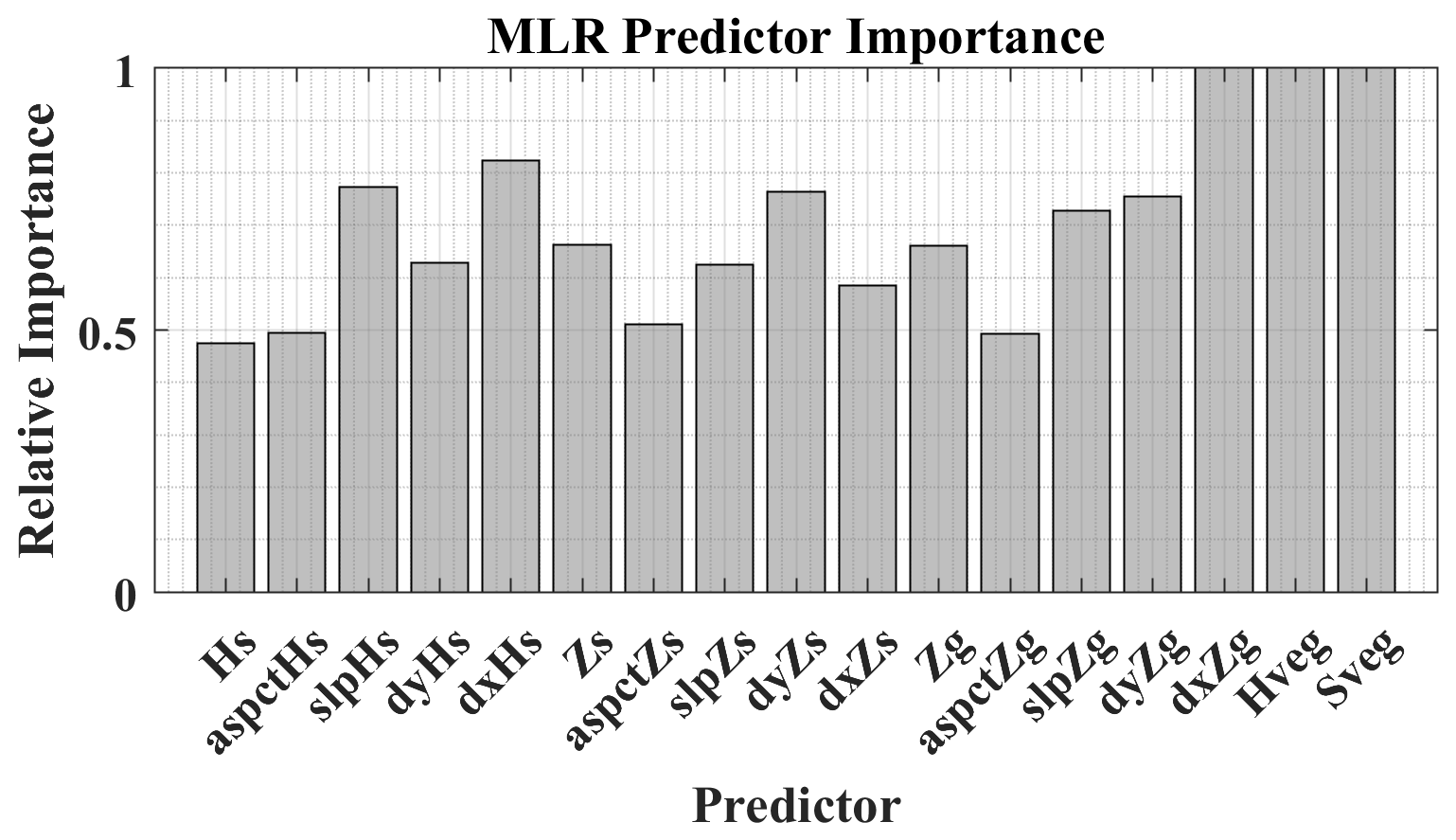
Figure A1The relative importance of the following lidar-derived predictors: Hs (snow depth), aspctHs (aspect of the snow depth), slpHs (slope of the snow depth), dyHs (north component of the snow depth gradient), dxHs (east component of the snow depth gradient), Zs (snow surface elevation) and its derivatives, Zg (ground elevation) and its derivatives, Hveg (vegetation height), and Sveg (distance to vegetation with a height greater than 0.5 m). The predictor importance was determined from the top 1 % of the models.
A2.2 Random-forest regression
The permutation accuracy importance was calculated to determine which of the lidar-derived predictor variables are most valuable in predicting the response. The permutation importance was assessed by comparing the accuracy of the prediction for a given learner (tree) and then randomly permuting the predictor variable of interest and recalculating the prediction accuracy (Hapfelmeier et al., 2014). An important predictor will lose its predictive capability after a random permutation, while an unimportant predictor will be unaffected by the randomization. The prediction accuracy was calculated using “out-of-bag” observations that were excluded from the population used to build the decision tree (Breiman, 2001). The relative out-of-bag predictor importance for the ensemble of random forests generated using 10 trees with a minimum leaf size of 200 suggests that the slope of the snow depth, snow surface elevation, ground surface elevation, proximity to vegetation, and vegetation height are the five leading predictors of snow density (Fig. A2).
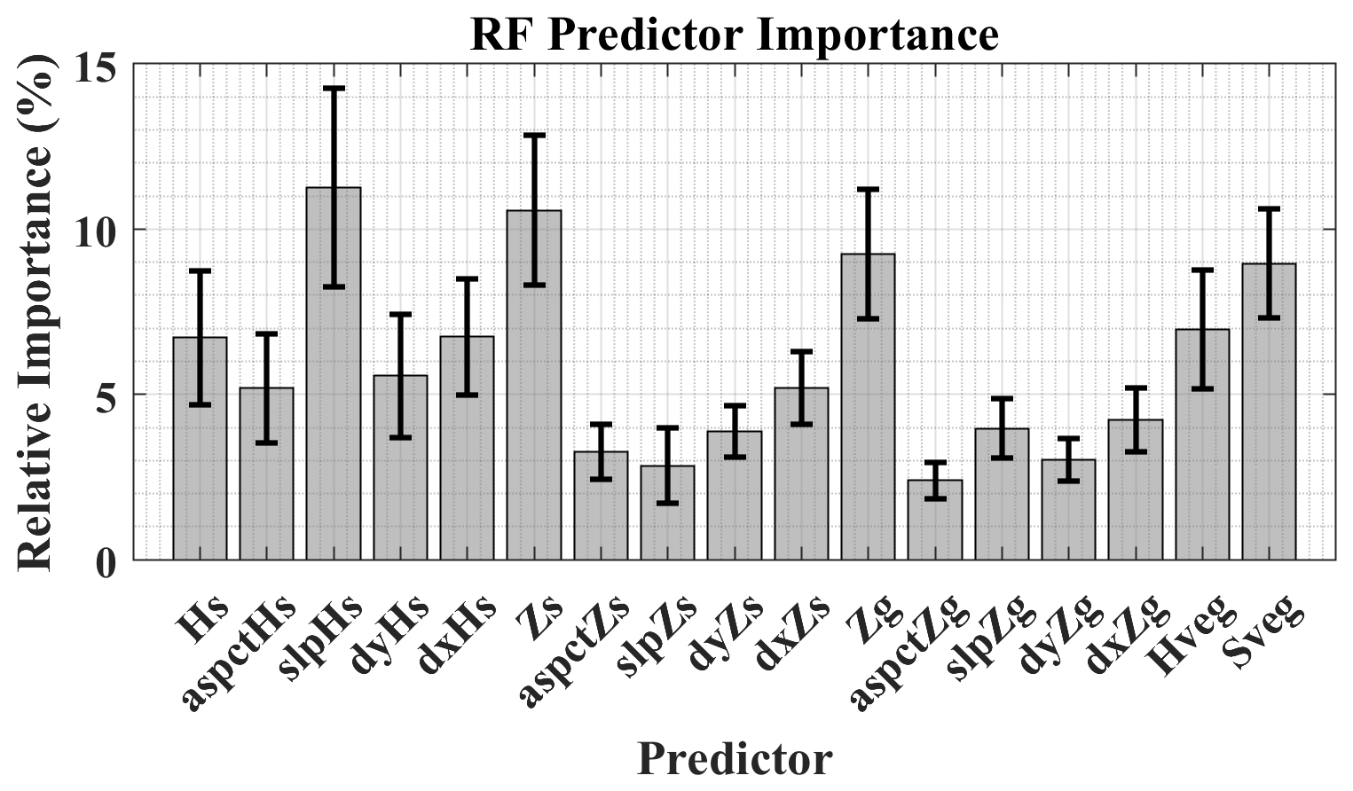
Figure A2Relative importance of lidar predictors calculated using the out-of-bag technique for random-forest regression. Uncertainties were developed using random subsets of training data in a Monte Carlo simulation.
A2.3 Artificial-neural-network regression
Approaches which partition the weights between neural connections to determine the relative importance of the predictors within an ANN have a classically simple architecture, with the network presenting one hidden layer (Goh, 1995). This technique becomes obfuscated when applying an ANN with multiple hidden layers. To determine the relative importance of predictors within an ensemble of networks with two hidden layers, we simply multiplied the matrices of the weights connecting the input to the first hidden layer, the first to the second hidden layer, and the second hidden layer to the output. The greater the overall weighting that is assigned to a predictor, the greater the importance of the feature. This method suggests that vegetation height, proximity to vegetation, the north derivative of the ground surface elevations, the slope of the ground elevations, and the east derivative of the snow surface elevations are the five leading predictors of snow density (Fig. A3).
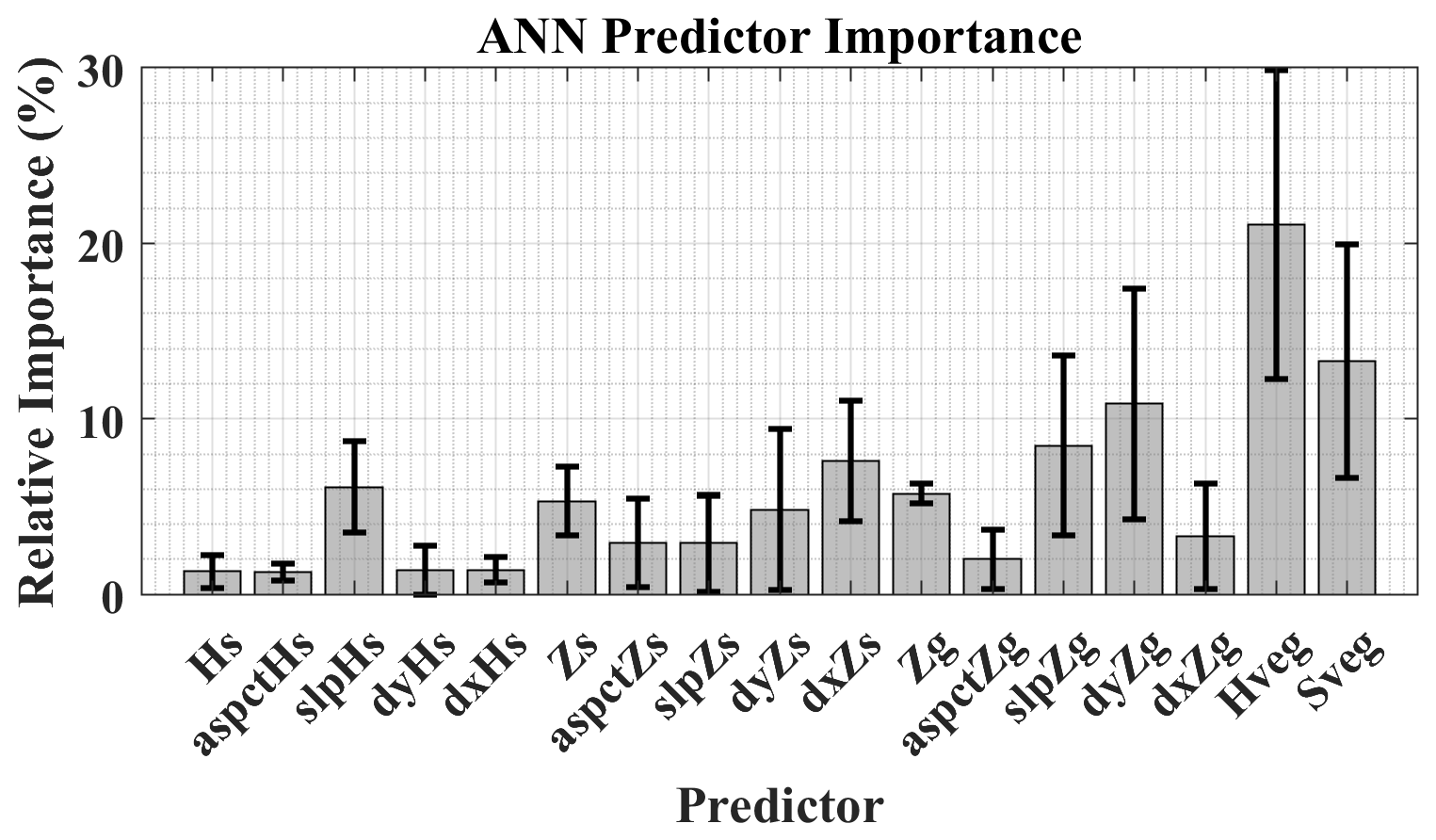
Figure A3Relative importance of lidar predictors within the ANN comprising two hidden layers.
A3 Model similarity intercomparison
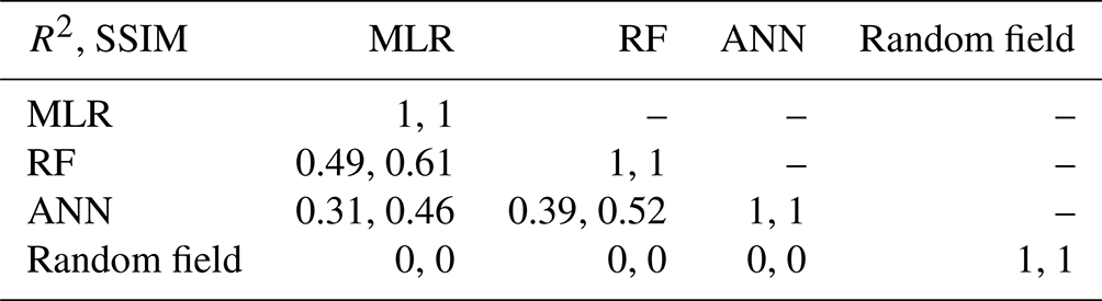
Visual inspection reveals apparent structural similarity among the three regression-based models. As a quantified model intercomparison, we applied the coefficient of determination measured by Pearson correlation calculated on a pixel-by-pixel basis. The structural similarity index (SSIM; Wang et al., 2004) is a normalized value between 0 and 1 that is defined by the image luminance, contrast, and standard deviation. We calculated the SSIM in 100 m radius kernels (comparable to the estimated correlation length of the density) as a second means of determining the similarity among the model ensembles. Capturing various structural length scales allows an examination of the model similarity across the correlation length. Table A1 overviews the R2 similarity matrix. Nearly 50 % of the features observed in the MLR model are explained within the RF model and vice versa. The SSIM similarity matrix suggests that there is greater structural similarity with a larger spatial support (Table A1). The random-field-synthesized model exhibits no repeatable structure and is uncorrelated with the various regression models – as expected, since it was randomly generated from the overall snow density statistics only.
Table A1Similarity matrix of R2 values for a pixel-by-pixel intercomparison, and SSIM values for a model intercomparison estimated over a 100 m radius (the approximate correlation length of snow density).
B1 Lidar point cloud processing
Point cloud processing was performed using the Multiscale Model to Model Cloud Compare method (Lague et al., 2013). The point cloud differencing method operates directly on point cloud data by selecting core points from the point clouds and distinguishing between the reference point cloud (representing the ground) and the compared point cloud (depicting snow-covered surfaces). Utilizing a user-defined radius denoted as D, the algorithm fits a plane within a radius of around each core point and determines the normal vector of the plane. Subsequently, based on the core point and the associated normal vector, the algorithm fits a cylinder with a radius of , oriented along the normal vector, with the cylinder axis passing through the core point. This cylinder intersects both the reference (ground) and compared (snow) point clouds, resulting in two sets of points. The algorithm then projects the points within each set onto the normal vector and calculates the average and standard deviation for each set. These values represent the average position and roughness, respectively. In the presence of outliers, the algorithm substitutes the mean and standard deviation with the median and interquartile range, respectively. Ultimately, the local distance between the average positions of the two sets provides the snow depth. However, in cases where surfaces are rough and the surface orientation does not align consistently with the normal direction, the measured distance (snow depth) uncertainty increases. This point cloud differencing method could prove beneficial for flat areas, given the effectiveness of the method on both rough and smooth surfaces.
The Cloud Compare Caractérisation de Nuages de Points (CANUPO) method was employed to distinguish vegetation from ground and snow returns following methods in Štroner et al., (2021). This process involves a combination of training and classification which defines the dimensionality of point clouds (1D for a line, 2D for a plane, or 3D for a volume) around specific points within a sphere at various scales (radii). The expectation is that branches exhibit a more linear (1D) structure, leaves display 2D surfaces at small scales (e.g., centimeter scales), and trees manifest in 3D at larger scales (e.g., meter scales). Both snow and ground surfaces tend to exhibit more of a 2D nature at both small and large scales. The determination of dimensionality is based on principal component analysis within the algorithm. The combination of point dimensionality at different scales is used to define object categories and, in this instance, remove vegetation.
B2 Error analysis of lidar–GPR-estimated density
We conducted a sensitivity analysis to evaluate how the errors in radar travel time and lidar snow depth affect the estimated snow density. This involved establishing a level curve through the average snow values of the study area (mean density 276 kg m−3, mean TWT 8 ns, and mean snow depth 96 cm) and applying perturbations to evaluate the density error (Fig. B1). Perturbations of up to ± 1 ns were added to the TWT and those of ± 15 cm were added to the depth. After the TWT and depth perturbations were applied, the densities were evaluated, and the mean (276 kg m−3) was subtracted from this result to measure the density perturbations. The error bars in Fig. B1 represent the lidar root-mean-square deviation evaluated by co-located depth probing (11 cm) and the RMSD of the GPR TWT crossovers (0.9 ns). At the 1σ level, errors of approximately ± 150 kg m−3 can be expected from this sensor integration method.
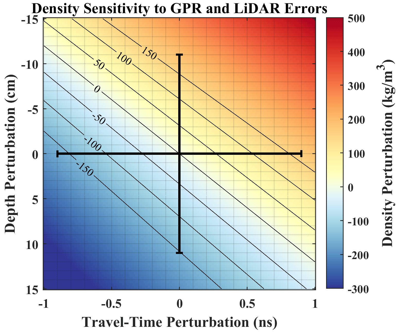
Figure B1Perturbations were added to the mean values of 8 ns for TWT and 96 cm for depth, and then the density was evaluated to estimate potential errors resulting from sensor integration (colored area and contours). The error bars represent the RMSE of the lidar (11 cm), evaluated by probing, and the RMSD of the GPR TWT crossovers (0.9 ns). At 1 standard deviation, combined snow density errors of ± 150 kg m−3 can be expected from sensor integration, which are reduced to within ± 30 kg m−3 by outlier filtering.
The combined measurement and geolocation errors in lidar-derived snow depths and GPR TWTs may translate into errors in the retrieved density that are larger than the range of densities observed in the snow pits. Upon filtering out outliers, the random error reduced to ± 30 kg m−3 and a meaningful density signal was retrieved. We chose the interquartile range of the lidar–GPR-retrieved densities as the threshold for determining outliers because the 25th and 75th percentiles envelop the range of snow densities observed in the snow pits. We then applied a 2D median window with a 12.5 m radius (chosen to extend beyond the correlation length of the errors) to smooth the densities and interpolate those at the outlying locations.
Although we only included GPR observations within 100 h of the 1 February lidar flight, seeking a potential bias related to the effects of densification and redistribution, we regressed ρs,lidar-GPR against hours elapsed prior to and after 1 February. Separate linear trends were identified in the forested and open regions traversed with the GPR. As conducted for the snow pit density observations, the trends were centered on 1 February and removed from the retrieved density observations.
B3 Statistics of the in situ, lidar–GPR-retrieved, and modeled snow densities
To show that the retrieved and modeled densities are within the range of measurements observed in the snow pits, we provide the distributions of these three datasets for the entire study area domain in Fig. B2. The means of the distributions overlap within the standard deviations of the datasets. The lidar–GPR-retrieved densities suggest a broader distribution of densities than those observed in the pits or modeled. Sampling biases may explain the small disagreement between mean values. The sample size and spatial representation of each dataset vary by many orders of magnitude. The distributions are unequally represented by vegetation class, as 18 % of the snow pits (17 of 96), 23 % of the modeled domain (3 665 343 of 15 753 500), and 7 % of the GPR transects (19 978 of 278 627) were located within the forest stands. However, other than a bias of - 10 kg m−3, the distribution of the modeled estimates closely resembles that of the snow pit measurements. Z tests confirm that the snow density data are normally distributed about the mean and the standard deviations are listed with high confidence.
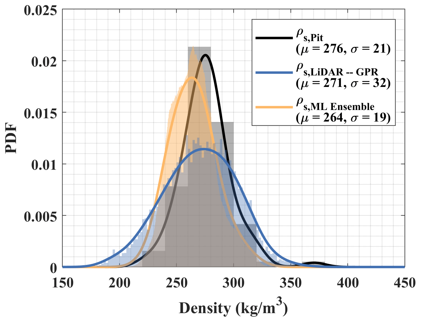
Figure B2Histograms of the snow-pit-measured, lidar–GPR-retrieved, and regression-model ensemble densities.
B4 Sample uncertainty of density and SWE
To estimate the uncertainty in average density due to the sample size and to propagate this uncertainty in terms of the SWE, we conducted Monte Carlo simulations by randomly subsampling density observations. Utilizing 1000 Monte Carlo realizations as a function of sample size, we incrementally increased the number of randomly sampled snow pits to estimate the mean and the standard deviation of the distributed average snow density (Fig. B3). We set the sampled standard deviation as the spatial uncertainty in density and summed in quadrature the distributed errors in lidar snow depth (as described in Sect. 2.7) to propagate the SWE uncertainty (Fig. B2). Our analysis suggests that 10 snow pit observations are sufficient to reduce the median uncertainty in SWE to within 10 ± 2 %.
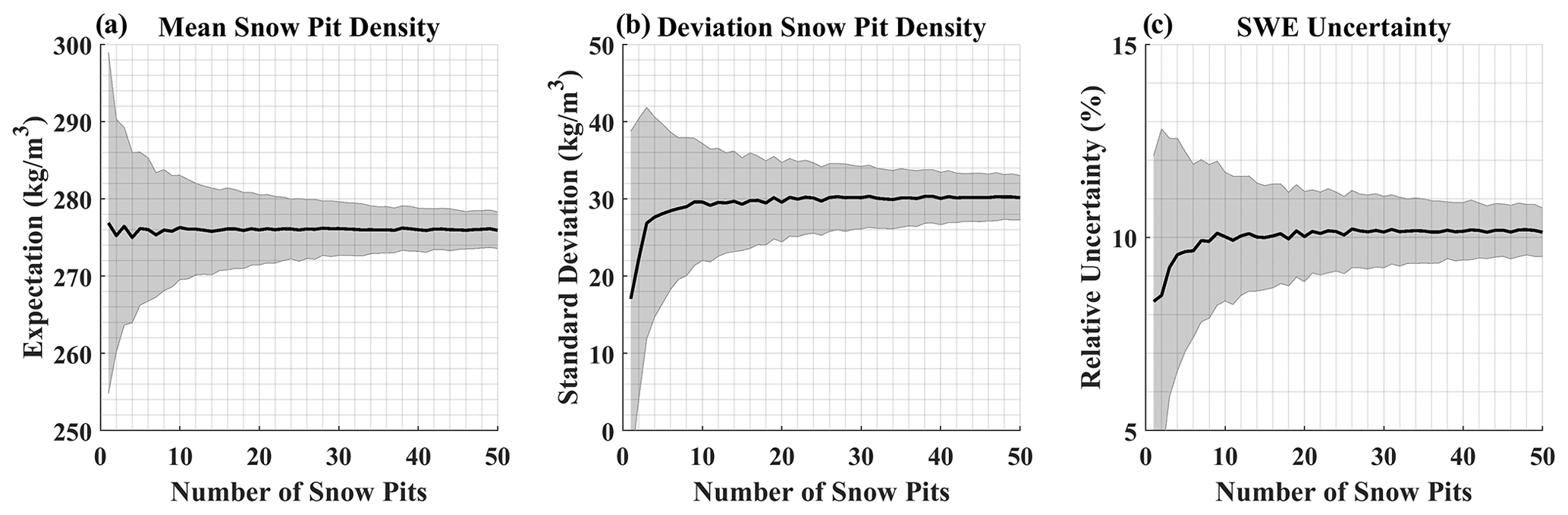
Figure B3Monte Carlo uncertainty analysis for (a) mean snow density, (b) the standard deviation of the snow density, and (c) the propagated SWE uncertainty as functions of sample size.
C1 Maximum upwind slope and wind factor
To infer the physical bases underlying the snow density patterns of , we computed two parameters (the maximum upwind slope and wind factor; Winstral et al., 2002) from the 1–2 February lidar-derived snow surface elevations. The maximum upwind slope characterizes the degree of wind exposure for a given pixel. A wind-sheltered pixel has a positive slope, indicating that higher terrain exists upwind of the pixel. Conversely, wind-exposed terrain has a negative slope value, with lower-elevation terrain in the upwind direction. The maximum upwind slope parameter (Sx) was calculated for each azimuth from 0 to 355° in 5° increments averaged over ± 15-degree overlapping bins (Winstral et al., 2002). A search distance of 25 m was applied in the calculation of the local Sx, while a 250 m distance was used to calculate the outlier length scale Sx between 25 and 250 m from the pixel. The local and outlying Sx parameters were differenced to calculate the slope break parameter, Sb (Winstral et al., 2002). Because pixels with high wind exposure have negative Sx values, and we hypothesize that wind-exposed terrain will have greater snow density (e.g., due to the formation of wind slabs), the wind direction expressing the largest negative correlation was recognized as the best explanation of the density patterns determined by Sx.
The wind-factor parameter determines the degree of wind exposure or shelter for a given pixel, based on Sx, Sb, vegetation proximity, and the average scalar multiple by which wintertime winds at the MW station exceeded those at the MM station (Winstral et al., 2002). The value of 2.18 determined from the wind speed data at MW and MM is in close agreement with the value of 2.3 determined by Winstral et al. (2002) and was applied to compute the wind factor by inversely rescaling Sx to the range between 1 and 2.18, where larger values indicate more wind exposure. Vegetated wind-sheltered zones were identified as pixels within a 3 m buffer of lidar vegetation greater than 0.5 m in height. The wind factors of sheltered vegetated areas and regions of Sb which exceeded the 97.5th percentile were arbitrarily reduced by 10 % to enhance the effective wind shelter provided by vegetation. Because the wind factor was inversely rescaled, the wind direction expressing the largest positive correlation with the snow density was recognized as being the best explanation of the density patterns determined by the wind factor parameter.
The processing software developed for the multi-polarization GPR analysis is available at https://doi.org/10.5281/zenodo.11521496 (Meehan, 2024).
Snow pit observations (https://doi.org/10.5067/DUD2VZEVBJ7S, Vuyovich et al., 2021), snow depth observations (https://doi.org/10.5067/9IA978JIACAR, Hiemstra et al., 2020), and GPR travel-time observations (https://doi.org/10.5067/Q2LFK0QSVGS2, Meehan, 2021; https://doi.org/10.5067/WE9GI1GVMQF6, Webb, 2021) acquired during the SnowEx 2020 Grand Mesa IOP are publicly available through the National Snow and Ice Data Center (NSIDC). Data products resulting from this work – the lidar–GPR-estimated density observations, the lidar-estimated model predictors, the modeled snow density, the modeled SWE (https://doi.org/10.5067/LANQ53RTJ2DR, Meehan and Hojatimalekshah, 2024a), and the lidar snow depth rasters (https://doi.org/10.5067/M9TPF6NWL53K, Meehan and Hojatimalekshah, 2024b) – and ASO snow depth (https://doi.org/10.5067/KIE9QNVG7HP0, Painter, 2018a) and SWE (https://doi.org/10.5067/M4TUH28NHL4Z, Painter, 2018b) data utilized comparatively in this work are also archived within the NSIDC.
The supplement related to this article is available online at: https://doi.org/10.5194/tc-18-3253-2024-supplement.
HPM, CH, and KE organized and led the SnowEx 2020 Grand Mesa IOP; TGM, AH, HPM, DM, RWW, RB, CH, and KE collected field measurements and curated various datasets utilized in this work; HPM, EJD, CH, and KE acquired funding for the field effort and labored to prepare this manuscript; TGM, AH, HPM, RB, MSR, and KE conceptualized the goals of this research; TGM developed the methodology, conducted the formal analysis, and prepared the manuscript; and all co-authors provided feedback on the manuscript through reviewing and editing.
The contact author has declared that none of the authors has any competing interests.
The findings of this document are not to be construed as an official Department of the Army position unless so designated by other authorized documents. The use of trade, product, or firm names in this document is for descriptive purposes only and does not imply endorsement by the U.S. Government.
Publisher's note: Copernicus Publications remains neutral with regard to jurisdictional claims made in the text, published maps, institutional affiliations, or any other geographical representation in this paper. While Copernicus Publications makes every effort to include appropriate place names, the final responsibility lies with the authors.
We wish to thank all the scientific participants and logistical support staff of the SnowEx 2020 campaign who helped make this research possible.
This research has been supported by the Engineer Research and Development Center (grant no. 601102/Project AB2/Task 1) and the Earth Sciences Division (grant nos. NNX17AL61G and 80NSSC18K0877).
This paper was edited by Florent Dominé and reviewed by Kat J. Bormann, César Deschamps-Berger, and one anonymous referee.
Andrews, D. F.: A robust method for multiple linear regression, Technometrics, 16, 523–531, https://doi.org/10.1080/00401706.1974.10489233, 1974.
Bentley, J. L.: Multidimensional Binary Search Trees Used for Associative Searching, Commun. ACM, 18, 509–517, https://doi.org/10.1145/361002.361007, 1975.
Besso, H., Shean, D., and Lundquist, J. D.: Mountain snow depth retrievals from customized processing of ICESat-2 satellite laser altimetry, Remote Sens. Environ., 300, 113 843, https://doi.org/10.1016/j.rse.2023.113843, 2024.
Bonnell, R., McGrath, D., Hedrick, A. R., Trujillo, E., Meehan, T. G., Williams, K., Marshall, H. P., Sexstone, G., Fulton, J., Ronayne, M. J., Fassnacht, S. R., Webb, R. W., and Hale, K. E.: Snowpack relative permittivity and density derived from near-coincident lidar and ground-penetrating radar, Hydrol. Process., 37, e14996, https://doi.org/10.1002/hyp.14996, 2023.
Bonner, H. M., Raleigh, M. S., and Small, E. E.: Isolating forest process effects on modelled snowpack density and snow water equivalent, Hydrol. Process., 36, e14475, https://doi.org/10.1002/hyp.14475, 2022.
Booth, A. D., Clark, R., and Murray, T.: Semblance response to a ground-penetrating radar wavelet and resulting errors in velocity analysis, Near Surf. Geophys., 8, 235–246. https://doi.org/10.3997/1873-0604.2010008, 2010.
Boyd, D. R., Alam, A. M., Kurum, M., Gurbuz, A. C., and Osmanoglu, B.: Preliminary Snow Water Equivalent Retrieval of SnowEX20 Swesarr Data, in: Proceedings of the 42nd IEEE International Symposium on Geoscience and Remote Sensing IGARSS, 17–22 July 2022, Kuala Lumpur, Malaysia, vol. 2022-July, ISBN 9781665427920, https://doi.org/10.1109/IGARSS46834.2022.9883412, pp. 3927–3930, 2022.
Breiman, L.: Random Forests, Mach. Learn., 45, 5–32, https://doi.org/10.1023/A:1010933404324, 2001.
Broxton, P. D., Leeuwen, W. J. D., and Biederman, J. A.: Improving Snow Water Equivalent Maps With Machine Learning of Snow Survey and Lidar Measurements, Water Resour. Res., 55, 3739–3757, https://doi.org/10.1029/2018WR024146, 2019.
Cressie, N.: Fitting variogram models by weighted least squares, J. Int. Ass. Math. Geol., 17, 563–586, https://doi.org/10.1007/BF01032109, 1985.
Deems, J. S., Fassnacht, S. R., and Elder, K. J.: Fractal Distribution of Snow Depth from Lidar Data, J. Hydrometeorol., 7, 285–297, https://doi.org/10.1175/JHM487.1, 2006.
Deems, J. S., Painter, T. H., and Finnegan, D. C.: Lidar measurement of snow depth: A review, J. Glaciol., 59, 467–479, https://doi.org/10.3189/2013JoG12J154, 2013.
Deschamps-Berger, C., Gascoin, S., Shean, D., Besso, H., Guiot, A., and López-Moreno, J. I.: Evaluation of snow depth retrievals from ICESat-2 using airborne laser-scanning data, The Cryosphere, 17, 2779–2792, https://doi.org/10.5194/tc-17-2779-2023, 2023.
Dewitz, J.: National Land Cover Database (NLCD) 2016 Products (ver. 3.0, November 2023), U.S. Geological Survey [data set], https://doi.org/10.5066/P96HHBIE, 2019.
Efron, B. and Tibshirani, R.: Bootstrap Methods for Standard Errors, Confidence Intervals, and Other Measures of Statistical Accuracy, Stat. Sci., 1, 77–77, https://doi.org/10.1214/ss/1177013817, 1986.
Elder, K., Dozier, J., and Michaelsen, J.: Snow accumulation and distribution in an Alpine Watershed, Water Resour. Res., 27, 1541–1552, https://doi.org/10.1029/91WR00506, 1991.
Elder, K., Rosenthal, W., and Davis, R. E.: Estimating the spatial distribution of snow water equivalence in a montane watershed, Hydrol. Process., 12, 1793–1808, https://doi.org/10.1002/(SICI)1099-1085(199808/09)12:10/11<1793::AID-HYP695>3.0.CO;2-K, 1998.
Essery, R., Morin, S., Lejeune, Y., and Ménard, C. B.: A comparison of 1701 snow models using observations from an alpine site, Adv. Water Resour., 55, 131–148, https://doi.org/10.1016/j.advwatres.2012.07.013, 2013.
Fassnacht, S. R., Heun, C. M., López-Moreno, J., and Latron, J.: Snow Density Variability in the Rio Esera Valley, Pyrenees Mountains, 2. Study Site, Cuadernos de Ivestigación Geográfica, 36, 59–72, 2010.
Goh, A.: Back-propagation neural networks for modeling complex systems, Artif. Intell. Eng., 9, 143–151, https://doi.org/10.1016/0954-1810(94)00011-S, 1995.
Griessinger, N., Mohr, F., and Jonas, T.: Measuring snow ablation rates in alpine terrain with a mobile multioffset ground-penetrating radar system, Hydrol. Process., 32, 3272–3282, https://doi.org/10.1002/hyp.13259, 2018.
Hapfelmeier, A., Hothorn, T., Ulm, K., and Strobl, C.: A new variable importance measure for random forests with missing data, Stat. Comput., 24, 21–34, https://doi.org/10.1007/s11222-012-9349-1, 2014.
Hedrick, A. R., Marks, D., Havens, S., Robertson, M., Johnson, M., Sandusky, M., Marshall, H., Kormos, P. R., Bormann, K. J., and Painter, T. H.: Direct Insertion of NASA Airborne Snow Observatory-Derived Snow Depth Time Series Into the iSnobal Energy Balance Snow Model, Water Resour. Res., 54, 8045–8063, https://doi.org/10.1029/2018WR023190, 2018.
Hiemstra, C., Marshall, H., Vuyovich, C., Elder, K., Mason, M., and Durand, M.: SnowEx20 Community Snow Depth Probe Measurements, Version 1, NASA National Snow and Ice Data Center Distributed Active Archive Center [data set], https://doi.org/10.5067/9IA978JIACAR, 2020.
Hiemstra, C. A., Vuyovich, C. M., and Marshall, H.-P.: SnowEx20 Grand Mesa Reference GIS Data Sets, Version 1, NASA National Snow and Ice Data Center Distributed Active Archive Center [data set], https://doi.org/10.5067/YDZXY4Q79VIJ, 2021.
Hill, D. F., Burakowski, E. A., Crumley, R. L., Keon, J., Hu, J. M., Arendt, A. A., Wikstrom Jones, K., and Wolken, G. J.: Converting snow depth to snow water equivalent using climatological variables, The Cryosphere, 13, 1767–1784, https://doi.org/10.5194/tc-13-1767-2019, 2019.
Hojatimalekshah, A., Uhlmann, Z., Glenn, N. F., Hiemstra, C. A., Tennant, C. J., Graham, J. D., Spaete, L., Gelvin, A., Marshall, H.-P., McNamara, J. P., and Enterkine, J.: Tree canopy and snow depth relationships at fine scales with terrestrial laser scanning, The Cryosphere, 15, 2187–2209, https://doi.org/10.5194/tc-15-2187-2021, 2021.
Houser, P., Rudisill, W., Johnston, J., Elder, K., Marshall, H., Vuyovich, C. M., Kim, E. J., and Mason, M.: SnowEx Meteorological Station Measurements from Grand Mesa, CO, Version 1, Boulder, Colorado USA, NASA National Snow and Ice Data Center Distributed Active Archive Center [data set], https://doi.org/10.5067/497NQVJ0CBEX, 2022.
Hu, X., Hao, X., Wang, J., Huang, G., Li, H., and Yang, Q.: Can the Depth of Seasonal Snow be Estimated From ICESat-2 Products: A Case Investigation in Altay, Northwest China, IEEE Geosci Remote S., 19, 1–5, https://doi.org/10.1109/LGRS.2021.3078805, 2021.
Isaaks, E. H. and Srivastava, R. M.: Applied Geostatistics, Oxford University Press, New York, NY, ISBN 9780195050134, 1989.
Jain, A., Mao, J., and Mohiuddin, K.: Artificial neural networks: a tutorial, Computer, 29, 31–44, https://doi.org/10.1109/2.485891, 1996.
Jonas, T., Marty, C., and Magnusson, J.: Estimating the snow water equivalent from snow depth measurements in the Swiss Alps, J. Hydrol., 378, 161–167, https://doi.org/10.1016/j.jhydrol.2009.09.021, 2009.
Kahaner, D., Moler, C., and Nash, S.: Numerical methods and software, Prentice Hall, Englewood Cliffs, ISBN 0-13-627258-4, 1989.
Kim, J. H., Cho, S. J., and Yi, M. J.: Removal of ringing noise in GPR data by signal processing, Geosci. J., 11, 75–81, https://doi.org/10.1007/BF02910382, 2007.
Kuwahara, M., Hachimura, K., Eiho, S., and Kinoshita, M.: Processing of RI-Angiocardiographic Images, Springer US, Boston, MA, https://doi.org/10.1007/978-1-4684-0769-3_13, 187–202, 1976.
Lague, D., Brodu, N., and Leroux, J.: Accurate 3D comparison of complex topography with terrestrial laser scanner: Application to the Rangitikei canyon (NZ), ISPRS J. Photogramm., 82, 10–26, https://doi.org/10.1016/j.isprsjprs.2013.04.009, 2013.
Lettenmaier, D. P., Alsdorf, D., Dozier, J., Huffman, G. J., Pan, M., and Wood, E. F.: Inroads of remote sensing into hydrologic science during the WRR era, Water Resour. Res., 51, 7309–7342, https://doi.org/10.1002/2015WR017616, 2015.
Li, L. and Pomeroy, J. W.: Estimates of Threshold Wind Speeds for Snow Transport Using Meteorological Data, J. Appl. Meteorol., 36, 205–213, https://doi.org/10.1175/1520-0450(1997)036<0205:EOTWSF>2.0.CO;2, 1997.
Lievens, H., Demuzere, M., Marshall, H.-P., Reichle, R. H., Brucker, L., Brangers, I., de Rosnay, P., Dumont, M., Girotto, M., Immerzeel, W. W., Jonas, T., Kim, E. J., Koch, I., Marty, C., Saloranta, T., Schöber, J., and Lannoy, G. J. M. D.: Snow depth variability in the Northern Hemisphere mountains observed from space, Nat. Commun., 10, 4629, https://doi.org/10.1038/s41467-019-12566-y, 2019.
Lievens, H., Brangers, I., Marshall, H.-P., Jonas, T., Olefs, M., and De Lannoy, G.: Sentinel-1 snow depth retrieval at sub-kilometer resolution over the European Alps, The Cryosphere, 16, 159–177, https://doi.org/10.5194/tc-16-159-2022, 2022.
López-Moreno, J. I., Fassnacht, S. R., Heath, J. T., Musselman, K. N., Revuelto, J., Latron, J., Morán-Tejeda, E., and Jonas, T.: Small scale spatial variability of snow density and depth over complex alpine terrain: Implications for estimating snow water equivalent, Adv. Water Resour., 55, 40–52, https://doi.org/10.1016/j.advwatres.2012.08.010, 2013.
Lukas, V. and Baez, V.: 3D Elevation Program—Federal best practices, U. S. Geological Survey Fact Sheet 2020–3062, U.S. Geological Survey, https://doi.org/10.3133/fs20203062, 2021.
Lv, Z. and Pomeroy, J. W.: Assimilating snow observations to snow interception process simulations, Hydrol. Process., 34, 2229–2246, https://doi.org/10.1002/hyp.13720, 2020.
Marks, D., Dozier, J., and Davis, R. E.: Climate and energy exchange at the snow surface in the Alpine Region of the Sierra Nevada: 1. Meteorological measurements and monitoring, Water Resour. Res., 28, 3029–3042, https://doi.org/10.1029/92WR01482, 1992.
Marshall, H., Vuyovich, C., Hiemstra, C., Brucker, L., Elder, K., Deems, J., Newlin, J., Bales, R., Nolin, A., and Trujillo, E.: NASA SnowEx 2020 Experiment Plan, NASA, https://snow.nasa.gov/campaigns/snowex/experimental-plan-2020 (last access: 7 June 2024), pp. 1–100, 2019.
Marshall, H. P., Koh, G., Sturm, M., Johnson, J. B., Demuth, M., Landry, C., Deems, J. S., and Gleason, J. A.: Spatial variability of the snowpack: Experiences with measurements at a wide range of length scales with several different high precision instruments, in: Proceedings ISSW 2006, International Snow Science Workshop, Telluride CO, USA, 1–6 October 2006, http://arc.lib.montana.edu/snow-science/item/947 (last access: 7 June 2024), pp. 359–364, 2006.
Marti, R., Gascoin, S., Berthier, E., de Pinel, M., Houet, T., and Laffly, D.: Mapping snow depth in open alpine terrain from stereo satellite imagery, The Cryosphere, 10, 1361–1380, https://doi.org/10.5194/tc-10-1361-2016, 2016.
McCreight, J. L. and Small, E. E.: Modeling bulk density and snow water equivalent using daily snow depth observations, The Cryosphere, 8, 521–536, https://doi.org/10.5194/tc-8-521-2014, 2014.
McGrath, D., Webb, R., Shean, D., Bonnell, R., Marshall, H. P., Painter, T. H., Molotch, N. P., Elder, K., Hiemstra, C., and Brucker, L.: Spatially Extensive Ground-Penetrating Radar Snow Depth Observations During NASA's 2017 SnowEx Campaign: Comparison With In Situ, Airborne, and Satellite Observations, Water Resour. Res., 55, 10026–10036, https://doi.org/10.1029/2019WR024907, 2019.
McGrath, D., Bonnell, R., Zeller, L., Olsen-Mikitowicz, A., Bump, E., Webb, R., and Marshall, H.-P.: A Time Series of Snow Density and Snow Water Equivalent Observations Derived From the Integration of GPR and UAV SfM Observations, Frontiers in Remote Sensing, 3, 1–15, https://doi.org/10.3389/frsen.2022.886747, 2022.
Meehan, T. G.: SnowEx20 Grand Mesa IOP BSU 1 GHz Multi-polarization GPR, Version 1, NASA National Snow and Ice Data Center Distributed Active Archive Center [data set], https://doi.org/10.5067/Q2LFK0QSVGS2, 2021.
Meehan, T.: tatemeehan/SnowEx2020_BSU_pE_GPR: Multipolarization Radargram Processing SnowEx 2020 Grand Mesa IOP (v1.0.0), Zenodo [code], https://doi.org/10.5281/zenodo.11521496, 2024.
Meehan, T. G. and Hojatimalekshah, A.: SnowEx20 Grand Mesa IOP Lidar and GPR-Derived Snow Water Equivalent and Snow Density, Version 1, NASA National Snow and Ice Data Center Distributed Active Archive Center [data set], https://doi.org/10.5067/LANQ53RTJ2DR, 2024a.
Meehan, T. G. and Hojatimalekshah, A.: SnowEx20 Grand Mesa IOP QSI Lidar Snow Depth Data, Version 1, NASA National Snow and Ice Data Center Distributed Active Archive Center [data set], https://doi.org/10.5067/M9TPF6NWL53K, 2024b.
Meehan, T. G., Marshall, H. P., Bradford, J. H., Hawley, R. L., Overly, T. B., Lewis, G., Graeter, K., Osterberg, E., and McCarthy, F.: Reconstruction of historical surface mass balance, 1984–2017 from GreenTrACS multi-offset ground-penetrating radar, J. Glaciol., 67, 219–228, https://doi.org/10.1017/jog.2020.91, 2021.
Meløysund, V., Leira, B., Høiseth, K. V., and Lisø, K. R.: Predicting snow density using meteorological data, Meteorol. Appl., 14, 413–423, https://doi.org/10.1002/met.40, 2007.
Mote, P. W., Li, S., Lettenmaier, D. P., Xiao, M., and Engel, R.: Dramatic declines in snowpack in the western US, NPJ Clim. Atmos. Sci., 1, 2, https://doi.org/10.1038/s41612-018-0012-1, 2018.
National Academies of Sciences Engineering and Medicine: Thriving on Our Changing Planet: A Decadal Strategy for Earth Observation from Space, National Academies Press, Washington, D.C., ISBN 978-0-309-46757-5, https://doi.org/10.17226/24938, 2018.
Neidell, N. S. and Taner, M. T.: Semblance and Other Coherency Measrues for Multichannel Data, Geophysics, 36, 482–497, https://doi.org/10.1190/1.1440186, 1971.
NOAA: VDatum 4.3 Vertical Datum Transformation, National Ocean Service NOAA Department of Commerce [software], https://vdatum.noaa.gov/ (last access: 7 June 2024), 2021.
Painter, T.: ASO L4 Lidar Snow Depth 3m UTM Grid, Version 1, NASA National Snow and Ice Data Center Distributed Active Archive Center [data set], https://doi.org/10.5067/KIE9QNVG7HP0, 2018a.
Painter, T.: ASO L4 Lidar Snow Water Equivalent 50m UTM Grid, Version 1, NASA National Snow and Ice Data Center Distributed Active Archive Center [data set], https://doi.org/10.5067/M4TUH28NHL4Z, 2018b.
Painter, T. H. and Bormann, K. J.: ASO L4 Lidar Point Cloud Digital Terrain Model 3 m UTM Grid, Version 1, NASA National Snow and Ice Data Center Distributed Active Archive Center [data set], https://doi.org/10.5067/2EHMWG4IT76O, 2020.
Painter, T. H., Berisford, D. F., Boardman, J. W., Bormann, K. J., Deems, J. S., Gehrke, F., Hedrick, A., Joyce, M., Laidlaw, R., Marks,D., Mattmann, C., McGurk, B., Ramirez, P., Richardson, M., Skiles, S. M. K., Seidel, F. C., and Winstral, A.: The Airborne Snow Observatory: Fusion of scanning lidar, imaging spectrometer, and physically-based modeling for mapping snow water equivalent and snow albedo, Remote Sens. Environ., 184, 139–152, https://doi.org/10.1016/j.rse.2016.06.018, 2016.
Pierce, D. W., Barnett, T. P., Hidalgo, H. G., Das, T., Bonfils, C., Santer, B. D., Bala, G., Dettinger, M. D., Cayan, D. R., Mirin, A., Wood, A. W., and Nozawa, T.: Attribution of declining Western U. S. Snowpack to human effects, J. Climate, 21, 6425–6444, https://doi.org/10.1175/2008JCLI2405.1, 2008.
Raleigh, M. S. and Small, E. E.: Snowpack density modeling is the primary source of uncertainty when mapping basin-wide SWE with lidar, Geophys. Res. Lett., 44, 3700–3709, https://doi.org/10.1002/2016GL071999, 2017.
Rovansek, R. J., Kane, D. L., and Hinzman, L. D.: Improving estimates of snowpack water equivalent using double sampling, in: Proceedings 61st Western Snow Conference, 9–11 June 1993, Quebec City, Quebec, pp. 157–163, 1993.
Siirila-Woodburn, E. R., Rhoades, A. M., Hatchett, B. J., Huning, L. S., Szinai, J., Tague, C., Nico, P. S., Feldman, D. R., Jones, A. D., Collins, W. D., and Kaatz, L.: A low-to-no snow future and its impacts on water resources in the western United States, Nat. Rev. Earth Environ., 2, 800–819, https://doi.org/10.1038/s43017-021-00219-y, 2021.
Singh, S., Durand, M., Kim, E., Pan, J., Kang, D. H., and Barros, A. P.: A Physical-Statistical Retrieval Framework to Estimate SWE from X and Ku-Band SAR Observations, vol. 2023-July, 16–21 July 2023, Pasadena, CA, USA, IEEE, ISBN 9798350320107, https://doi.org/10.1109/IGARSS52108.2023.10281838, pp. 17–20, 2023.
Sturm, M. and Holmgren, J.: Differences in compaction behavior of three climate classes of snow, Ann. Glaciol., 26, 125 130, https://doi.org/10.3189/1998AoG26-1-125-130, 1998.
Sturm, M., Taras, B., Liston, G. E., Derksen, C., Jonas, T., and Lea, J.: Estimating snow water equivalent using snow depth data and climate classes, J. Hydrometeorol., 11, 1380–1394, https://doi.org/10.1175/2010JHM1202.1, 2010.
Štroner, M., Urban, R., Lidmila, M., Kolář, V., and Křemen, T.: Vegetation Filtering of a Steep Rugged Terrain: The Performance of Standard Algorithms and a Newly Proposed Workflow on an Example of a Railway Ledge, Remote Sens.-Basel, 13, 3050, https://doi.org/10.3390/rs13153050, 2021.
Tedesco, M., Reichle, R., Low, A., Markus, T., and Foster, J. L.: Dynamic Approaches for Snow Depth Retrieval From Spaceborne Microwave Brightness Temperature, IEEE T. Geosci. Remote, 48, 1955–1967, https://doi.org/10.1109/TGRS.2009.2036910, 2010.
Tiuri, M. E., Sihvola, A. H., Nyfors, E. G., and Hallikaiken, M. T.: The Complex Dielectric Constant of Snow at Microwave Frequencies, IEEE J. Oceanic Eng., 9, 377–382, https://doi.org/10.1109/JOE.1984.1145645, 1984.
Treichler, D. and Kääb, A.: Snow depth from ICESat laser altimetry — A test study in southern Norway, Remote Sens. Environ., 191, 389–401, https://doi.org/10.1016/j.rse.2017.01.022, 2017.
Trujillo, E., Ramírez, J. A., and Elder, K. J.: Scaling properties and spatial organization of snow depth fields in sub-alpine forest and alpine tundra, Hydrol. Process., 23, 1575–1590, https://doi.org/10.1002/hyp.7270, 2009.
Tsang, L., Durand, M., Derksen, C., Barros, A. P., Kang, D.-H., Lievens, H., Marshall, H.-P., Zhu, J., Johnson, J., King, J., Lemmetyinen, J., Sandells, M., Rutter, N., Siqueira, P., Nolin, A., Osmanoglu, B., Vuyovich, C., Kim, E., Taylor, D., Merkouriadi, I., Brucker, L., Navari, M., Dumont, M., Kelly, R., Kim, R. S., Liao, T.-H., Borah, F., and Xu, X.: Review article: Global monitoring of snow water equivalent using high-frequency radar remote sensing, The Cryosphere, 16, 3531–3573, https://doi.org/10.5194/tc-16-3531-2022, 2022.
US Census Bureau: Cartographic Boundary Files, US Census Bureau [data set], https://www.census.gov/geographies/mapping-files/time-series/geo/cartographic-boundary.html (last access: 7 June 2024), 2020.
Valence, E., Baraer, M., Rosa, E., Barbecot, F., and Monty, C.: Drone-based ground-penetrating radar (GPR) application to snow hydrology, The Cryosphere, 16, 3843–3860, https://doi.org/10.5194/tc-16-3843-2022, 2022.
Vecherin, S., Meyer, A., Quinn, B., Letcher, T., and Parker, M.: Simulation of Snow Texture for Autonomous Vehicle Numerical Modeling, National Defense Industrial Association, http://gvsets.ndia-mich.org/publication.php?documentID=928 (last access: 7 June 2024), 2022.
Vuyovich, C. M., Marshall, H., Elder, K., Hiemstra, C., Brucker, L., and McCormick, M.: SnowEx20 Grand Mesa Intensive Observation Period Snow Pit Measurements, Version 1, NASA National Snow and Ice Data Center Distributed Active Archive Center [data set], https://doi.org/10.5067/DUD2VZEVBJ7S, 2021.
Wang, Z., Bovik, A. C., Sheikh, H. R., and Simoncelli, E. P.: Image quality assessment: From error visibility to structural similarity, IEEE T. Image Process., 13, 600–612, https://doi.org/10.1109/TIP.2003.819861, 2004.
Webb, R. W.: SnowEx20 Grand Mesa IOP UNM 800 and 1600 MHz MALA GPR, Version 1, NASA National Snow and Ice Data Center Distributed Active Archive Center [data set], https://doi.org/10.5067/WE9GI1GVMQF6, 2021.
Webb, R. W., Marziliano, A., McGrath, D., Bonnell, R., Meehan, T. G., Vuyovich, C., and Marshall, H.-P.: In Situ Determination of Dry and Wet Snow Permittivity: Improving Equations for Low Frequency Radar Applications, Remote Sens.-Basel, 13, 4617, https://doi.org/10.3390/rs13224617, 2021.
Wetlaufer, K., Hendrikx, J., and Marshall, L.: Spatial heterogeneity of snow density and its influence on snow water equivalence estimates in a large mountainous basin, Hydrology, 3, 3, https://doi.org/10.3390/hydrology3010003, 2016.
Wharton, R. P., Hazen, G. A., Rau, R. N., and Best, D. L.: Advancements In Electromagnetic Propagation Logging, in: Proceedings Society of Petroleum Engineers Rocky Mountain Regional Meeting, 14–16 May 1980, Casper, Wyoming, Society of Petroleum Engineers, https://doi.org/10.2118/9041-MS, 1980.
Winstral, A., Elder, K., and Davis, R. E.: Spatial Snow Modeling of Wind-Redistributed Snow Using Terrain-Based Parameters, J. Hydrometeorol., 3, 524–538, https://doi.org/10.1175/1525-7541(2002)003<0524:SSMOWR>2.0.CO;2, 2002.
Wong, J., Han, L., Bancroft, J. C., and Stewart, R. R.: Automatic time-picking of first arrivals on noisy microseismic data, in: Proceedings Canadian Society of Exploration Geophysics Meeting, 13–15 October 2009, Olympic Park, Calgary, Canada, pp. 1–6, 2009.
Yildiz, S., Akyurek, Z., and Binley, A.: Quantifying snow water equivalent using terrestrial ground penetrating radar and unmanned aerial vehicle photogrammetry, Hydrol. Process., 35, 1–15, https://doi.org/10.1002/hyp.14190, 2021.
Yilmaz, Ö.: Seismic Data Analysis, Society of Exploration Geophysicists, Tulsa, OK, ISBN 978-1-56080-094-1, https://doi.org/10.1190/1.9781560801580, 2001.