the Creative Commons Attribution 4.0 License.
the Creative Commons Attribution 4.0 License.
 | 05 Jul 2024
Two-dimensional numerical simulations of mixing under ice keels
Sam De Abreu
Rosalie M. Cormier
Mikhail G. Schee
Varvara E. Zemskova
Erica Rosenblum
Nicolas Grisouard
Changes in sea ice conditions directly impact the way the wind transfers energy to the Arctic Ocean. The thinning and increasing mobility of sea ice is expected to change the size and speed of ridges on the underside of ice floes, called ice keels, which cause turbulence and impact upper-ocean stratification. However, the effects of changing ice keel characteristics on below-ice mixing are difficult to determine from sparse observations and have not been directly investigated in numerical or laboratory experiments. Here, for the first time, we examine how the size and speed of an ice keel affect the mixing of various upper-ocean stratifications using 16 two-dimensional numerical simulations of a keel moving through a two-layer flow. We find that the irreversible ocean mixing and the characteristic depth over which mixing occurs each vary significantly across a realistic parameter space of keel sizes, keel speeds, and ocean stratifications. Furthermore, we find that mixing does not increase monotonically with ice keel depth and speed but instead depends on the emergence and propagation of vortices and turbulence. These results suggest that changes to ice keel speed and depth may have a significant impact on below-ice mixing across the Arctic Ocean and highlight the need for more realistic numerical simulations and observational estimates of ice keel characteristics.
- Article
(3465 KB) - Full-text XML
- BibTeX
- EndNote


Wind-driven mixing in the Arctic Ocean directly affects the stratification of the upper ocean and, therefore, the vertical transfer of heat and the evolution of sea ice (Carmack et al., 2015; Rainville et al., 2011; MacKinnon et al., 2021; Timmermans and Marshall, 2020). Processes that drive mixing typically occur at spatiotemporal scales smaller than a climate model can resolve; hence, ocean mixing has to be parameterized. Despite its importance, the representation of ocean mixing in ice-covered waters is poorly constrained in climate models, potentially contributing to an unrealistic representation of the Arctic halocline in the past several generations of global ice–ocean models and coupled climate models (Holloway et al., 2007; Ilicak et al., 2016; Rosenblum et al., 2021; Barthélemy et al., 2015; Jin et al., 2012; Nguyen et al., 2009; Sidorenko et al., 2018). This may have direct implications for biases in simulated circulations of Pacific Water and Atlantic Water and ice–ocean heat fluxes (Zhang and Steele, 2007; Lavoie et al., 2021; Liang and Losch, 2018) and possibly sea ice retreat (Niederdrenk and Notz, 2018; Rosenblum and Eisenman, 2016, 2017; Notz and SIMIP Community, 2020; Stroeve et al., 2007, 2012; Winton, 2011).
Historically, multi-year sea ice shielded the majority of the underlying Arctic Ocean from the wind, leading to a relatively quiescent Arctic Ocean. However, during the period 1979–2018, the September ice cover receded by 45.2 % relative to 1979–1989 (Stroeve and Notz, 2018). The shrinkage of this “sea ice lid” has allowed the wind to interact directly with the ocean, increasing wind-driven momentum transfer into the ocean but yielding uncertain effects for vertical mixing (Rainville and Woodgate, 2009; Rainville et al., 2011; Rippeth et al., 2015; Lincoln et al., 2016; Brown et al., 2020; Guthrie and Morison, 2021; Dosser et al., 2021; Fine and Cole, 2022).
But what happens below a thick, multi-year sea ice cover that is transitioning to thinner, first-year ice? Like a spoon in a glass of water, sea ice stirs and mixes the ocean differently, depending on its shape and speed. Observations indicate that the shapes and speeds of sea ice have undergone significant changes over the past few decades. The proportion of multi-year to first-year sea ice has declined from 59 % in 1984 to 28 % in 2018 (Stroeve and Notz, 2018), resulting in a sea ice pack that is on average thinning (Kwok and Rothrock, 2009; Rampal et al., 2011; Kwok, 2018; Meier and Stroeve, 2022; Sumata et al., 2023), becoming more mobile with faster drift speeds (Rampal et al., 2009; F. Zhang et al., 2022) and shallower ridges (Wadhams, 2012; Hutchings and Faber, 2018; Kwok, 2018), consisting of smaller ice floes (Hutchings and Faber, 2018), and undergoing large regional and temporal variations in roughness (Tsamados et al., 2014).
Using global ice–ocean model simulations, Martin et al. (2016) demonstrated that the shape of sea ice matters as much as its speed to explain the decadal basin-wide changes in wind-driven momentum transfer into the ocean. Specifically, they found that the inclusion of changes in the roughness of sea ice, modeled as sea ice keels (deep pressure ridges underneath ice floes) and sails (the keels' above-ice counterparts), caused ocean surface stress to decrease by 3.1 % per decade. In contrast, simulations that ignore changes in sea ice roughness, such as most climate models, simulate an ocean surface stress that increases by 4.6 % per decade. This sensitivity to sea ice roughness is qualitatively consistent with observational, numerical, and laboratory studies that indicate that sea ice bottom roughness is important for kinetic energy dissipation, vertical mixing (Fer and Sundfjord, 2007; Fer et al., 2022; McPhee, 1983), internal wave generation (Cole et al., 2018; McPhee and Kantha, 1989), and ice–ocean drag (Cole et al., 2017; Brenner et al., 2021; Pite et al., 1995; Zu et al., 2021; McPhee, 2012), and it has direct implications for ice–ocean turbulent heat fluxes (Randelhoff et al., 2014; Skyllingstad et al., 2003).
Oceanographic studies suggest that ice keels cause significant turbulence that should have a large impact on the summer pycnocline. In situ observations by Fer and Sundfjord (2007) and Fer et al. (2022) report that the presence of keels yields deeper mixing and greater kinetic energy dissipation than would be expected if the ice were flat. Carr et al. (2019) and P. Zhang et al. (2022) ran numerical experiments of internal solitary waves (nonlinear, non-hydrostatic oscillations of the pycnocline) impinging on floe edges and ice keels, respectively, reporting that this interaction can result in the creation of secondary waves and turbulence. Using three-dimensional large-eddy simulations inspired by Arctic observations, Skyllingstad et al. (2003) estimated that ice keels could enhance vertical heat fluxes by factors of 3 to 10 but did not distinguish between reversible fluxes (i.e., adiabatic stirring of water parcels) and irreversible fluxes (i.e., diabatic mixing of waters of different densities). This distinction matters for climate models because the latter has long-term impacts on the stratification of the upper ocean, while the former does not. Here, for the first time, we directly investigate the relative impacts of ice keel size and speed on diabatic turbulent ocean mixing.
Accurate representations of the impact of sea ice roughness on ocean mixing in climate model parameterizations will require a fundamental understanding of how the variability in ice keels' sizes and shapes affects mixing in the upper ocean. How ice-keel-like objects interact with Arctic-like summer mixed layers has, to our knowledge, been the topic of relatively few process studies. In this article, we explore keel-driven mixing considering a range of ice keel depths, ice keel speeds, and summer upper-ocean stratifications that are representative of previous observations in the Arctic using a suite of two-dimensional numerical experiments.
In Sect. 2, we describe how we adapt several previous approaches to characterize our numerical simulation setup in the context of ice keel stirring and mixing, as well as the governing equations, and our approach to quantifying mixing. In Sect. 3, we categorize different stirring regimes upstream and downstream of the keel for each simulation.
Intuitively, we could expect faster, deeper keels to generate more diapycnal mixing over a larger depth range (hereafter referred to as the null hypothesis). However, relatively deep keels can also act to inhibit mixing by blocking flow ahead (upstream) of the keel. Similarly, relatively fast keels can act to inhibit mixing by generating a localized boundary layer, allowing laminar flow above to move past the keel with little interaction between layers of different density or with the keel. We use our stirring regime categorization to interpret variations away from the null hypothesis and present the magnitude and vertical extent of mixing in Sect. 4. We further discuss and summarize, putting our results in the context of the Arctic Ocean, in Sects. 5 and 6.
2.1 Governing equations
We use an idealized two-layer model to simulate the cross-sectional motion of fluid around an ice keel. Figure 1 shows each element of our setup, which we expand on in the rest of this section. Our equations and code are adapted from Hester et al. (2021), who simulated a single-layer fluid flow across an iceberg at the surface to examine the influence of its aspect ratio on melt. Our specific adaptations are the use of a two-layer rather than one-layer stratification, an adjustment of the shape of the obstacle to simulate an ice keel rather than an iceberg, the inclusion of a gradual acceleration of the obstacle, the removal of all possible phase changes of water, and the removal of temperature dependence from the governing equations. We ignore Coriolis terms because our timescale and length scale are small (tens of minutes and tens of meters, respectively). Note that one does not need to go far from the ice boundary (a couple meters for typical surface stresses) before rotation can influence the mixing length (McPhee, 2012); however, our timescales are sufficiently short (shorter than an inertial period) to neglect rotational effects.

Figure 1A schematic of our setup, which consists of a mixed layer (dark blue) initialized over z≤z0 with density ρ1; a deeper-ocean layer (yellow) with density ρ2; and an ice keel (white) of draft h, characteristic width σ, and phase field ϕ=1 located at x=ℓ. Dashed lines indicate the upstream region () and downstream region (), both of which extend down the entire water column while excluding the keel. Sponge layers ( and ), denoted by ψ, and their associated governing equations are also indicated.
The resulting governing equations form a set of non-hydrostatic salinity advection–diffusion equations with fluid velocity, pressure, and density fluctuations that satisfy the Boussinesq equations, namely
along with the EOS-80 equation of state (Fofonoff and Millard, 1983) that relates the density ρ to the salinity S, assuming a constant temperature of −2 °C. Here, x is the horizontal distance from the left boundary; z is the vertical distance from the surface (i.e., it increases positively downward); u and w are the horizontal and vertical velocity components, respectively; p is the scaled pressure fluctuation field; Si is the initial salinity field (see Eq. 5); is the spanwise vorticity; U is the keel velocity relative to the fluid; and . The equations are written in a computationally advantageous form by decomposing the advection term into the sum of the Lamb vector and a gradient term incorporated into the pressure gradient. Kinematic viscosity ν and the salt-mass diffusivity μ are both of value m2 s−1. We choose such large values for ν and μ to dissipate eddies smaller than the resolution of the grid, similar to the choice of P. Zhang et al. (2022), which keeps our numerical cost tractable. These values may have quantitative consequences on mixing but should preserve our qualitative conclusions, as we discuss in Sect. 5.2. The fields ϕ and ψ are masks for the keel and sponge layers (see below), ξ=7.1 ms is the damping and restoring timescale associated with ϕ and ψ, and regulates the salinity equation within the keel.
The two-layer fluid has an initial salinity profile Si(x,z), which consists of an upper layer of salinity S1 and density ρ1=ρ(S1), which we call the “mixed layer”, overlying a deeper layer of salinity S2 and density , which we call the “deeper ocean”. The mixed layer extends to a depth of z0 with a narrow halocline transition to the deeper-ocean layer. The initial salinity profile is
where H(x) is the location of the keel boundary, which we define below; ; and b=0.1 m.
Inside the keel, the salinity is maintained at S1, the initial salinity of the mixed layer. The smooth phase field ϕ(x,z) marks the location of the keel. That is to say that it satisfies ϕ=1 inside the keel and ϕ=0 outside, with a sigmoidal transition over a distance ε across the boundary. Note that the keel does not melt and simulations occur in a reference frame that moves with the keel, i.e., . The geometries of ice keels in the Arctic Ocean are rather complicated and can vary greatly due to the nature of their formation. Computational models typically employ cosine, Gaussian, triangular, and Versoria functions to define the shapes of keels (P. Zhang et al., 2022). To maintain consistency with previous ice keel simulations (Skyllingstad et al., 2003; Mortikov, 2016; Pite et al., 1995), we use a Versoria shape of the form
where h is the maximum ice keel draft, σ is the characteristic width of the keel, and ℓ=75z0 is the center of the keel.
At the left and right ends of the domain, sponge layers (identified by their prefactors ψ in Eqs. 1–3) restore the horizontal velocity of the fluid u to a constant U, restore the salinity S to Si, and damp the vertical velocity w. We set ψ=1 for x<2.5z0 and for x>117.5z0 and ψ=0 between them, with sigmoidal transitions over distances ε, similar to ϕ. The sponge layers are linearly accelerated from rest to a horizontal speed U in the first 15 min of simulation time and then maintained at U for the rest of the simulation (≈35–85 min; see below for details). At approximately 30 min in each simulation, the upstream sponge layers emit a small disturbance as a result of our implementation of the acceleration, akin to adding noise to simulations or the real ocean. Due to the nature of the two-layered flow, the disturbance amounts to a perturbation in the fluid interface, which travels downstream and, in some cases, triggers fluid instabilities along the way. Due to this ability to “ignite” unstable flows, we refer to this disturbance as the “pilot light”, which we will use in Sect. 3.1.
We solve Eqs. (1)–(4) with two-dimensional numerical simulations created in Dedalus, a spectral partial differential equation solver (Burns et al., 2020). We use a Fourier basis in the horizontal, making the domain horizontally periodic. In the vertical, the quantities u, p, S, and ϕ are decomposed on a cosine basis, producing homogeneous Neumann boundary conditions for these quantities (e.g., ), while w is decomposed on a sine basis, resulting in homogeneous Dirichlet boundary conditions (). Note that because the velocity is zero inside the keel, our setup imposes an effective no-slip boundary condition along the ice–water interface, the implications of which are discussed in Sect. 5.2. The terms on the left-hand side (right-hand side) of Eqs. (1)–(3) are treated implicitly (explicitly) with a third-order semi-implicit backward differentiation formula time-stepping scheme (Wang and Ruuth, 2008).
2.2 Parameter space and experimental strategy
From a fluid dynamics point of view, density mixing by ice keels falls into the rather well-studied area of two-layer flow over bottom topography (e.g., Baines, 1984; Holland et al., 2002). Similarly to our setup, these previous studies consider an obstacle that moves through two-layer fluid, causing stirring and, when miscible, irreversible mixing of the two initial densities. These previous studies indicated that one of the most important parameters characterizing the flow of this system is the Froude number, Fr, which is the ratio between the obstacle speed relative to the upper layer and the interfacial wave speed.
When the Froude number is low (typically less than unity) – i.e., when the keel is relatively slow or the density stratification is relatively strong – waves can propagate upstream and the resultant flow is called subcritical. Conversely, large Froude numbers (typically larger than unity) correspond to supercritical flows, and any flow feature such as a wave or vortex can only be swept downstream.
Based on a “bulk” Froude number, Baines (1984) further defined regimes based on the presence of flow characteristics. This included determining whether the flow was supercritical or subcritical, whether transitions between the two occurred, and whether disturbances such as bores or waves were able to propagate upstream. We will find some of these characteristics and regimes in Sect. 3.
Here, we examine five variables that govern the dynamics of the system: keel draft h, keel width σ, mixed-layer depth z0, buoyancy difference between the mixed layer and the deeper ocean , and horizontal keel speed relative to water U. Three independent non-dimensional parameters are sufficient to completely describe the dynamics controlled by these variables. Similarly to previous studies (e.g., Baines, 1984; Cummins, 1995; Houghton and Kasahara, 1968), we choose
namely the bulk Froude number, the non-dimensional keel draft, and the keel's aspect ratio, respectively. In our experiments, we will only vary two of these non-dimensional parameters, namely Fr and η. For each experiment, we set the aspect ratio α=3.9, based on observations showing that this value is consistent among first-year ice floes (no such consistency is apparent in multi-year ice) (Timco and Burden, 1997).
To obtain the permissible ranges of values for Fr and η, we establish bounds from observations of the Arctic Ocean. Ice keel drafts are, on average, 7.45 m but can reach depths of up to 45 m (Wadhams, 2012; Kvadsheim, 2014). For the depth of the mixed layer, we take , which is consistent with the observed range of summer mixed-layer depths across the Arctic Ocean (hereafter referred to as PFW; Peralta-Ferriz and Woodgate, 2015). In the marginal ice zone, Cole et al. (2017) estimate U≤0.4 m s−1. Lastly, we calculate the bounds of ΔB using the bounds of ΔS between the mixed summer and winter layers reported by PFW and use EOS-80 to calculate the respective densities. Note that this will yield larger ΔB values than those resulting from using the 0.1 kg m−3 density step from PFW, from which we obtained our mixed-layer depth. The discrepancy in ΔB results from our choice to define the densities ρ1 and ρ2 using summer and winter values, where – by contrast – PFW's criterion defines ρ2 using a value representing the transition between the summer and winter layers. We believe that the former better encapsulates summer conditions reminiscent of PFW's two-layer model (see their Fig. 9c).
With the upper and lower bounds on ρ1 and ρ2 thus calculated, we obtain . Thus, we find that
Simulations with Fr=2.5 could not run throughout the entire η range, nor could simulations with η>2 run throughout the entire Fr range, without encountering numerical instabilities. We therefore consider four values of η, namely 0.50, 0.95, 1.2, and 2.0, and four values of Fr, namely 0.5, 1.0, 1.5, and 2.0. We name our simulations based on their Fr and η values, following the convention F⌊10Fr⌋H⌊10η⌋, where ⌊⋅⌋ is the floor operator. For example, we refer to the Fr=0.5 and η=0.95 simulation as F05H09.
To vary Fr and η, we set z0=8 m, ΔB=0.015 m s−2, S1=28 psu, and S2=30 psu and, therefore, vary U and h through the respective ranges and , according to Eq. (7). These parameter choices yield Reynolds numbers ranging from O(102) to O(103). Note that we increase the phase field steepness parameter ε for η=2.0 simulations to prevent salinity leakage from the keel. See Table 1 for a summary of the parameter values for all simulations.
Table 1The values of all parameters for all 16 simulations. ε is the phase field steepness parameter, Re is the Reynolds number, and trt is the total run time of the simulation.

The simulation domain has height 10z0 and length 120z0. We focus our analysis on regions upstream and downstream of the keel, which we choose to be and , respectively, and that occupy the entire water column (see Fig. 1). For simulations with Fr<2.0, a stagnant layer forms upstream of the keel, and its spatial extent grows over time in the wake of an interfacial wave. This wave eventually reflects against the edge of the upstream sponge layer and propagates downstream. We consider processes that occur after this wave reach the upstream region at x=20z0 to be an artifact of our setup, marking the time when we stop processing data. We found that this time window varied more directly with Fr than with η. Consequently, measuring simulation time in units of (≈23 s), we stopped simulations with Fr=1.5 and Fr=2.0 at t=270t0, simulations with Fr=1.0 at t=156t0, and simulations with Fr=0.5 at t=132t0. Each simulation uses a time step of and a domain discretized with 1280 horizontal and 640 vertical grid points.
In some experiments, we observe vertical aliasing in the mixed and deep layers in the form of horizontal alternating bands in the spanwise vorticity q and vertical density gradients ∂zρ. This aliasing has no effect on the stability of the numerical integration. It does create artificially enhanced density mixing values in weakly stratified regions that we can easily remove from our diagnostic calculations (see below).
2.3 Quantifying mixing
To analyze the vertical mixing induced by the motion of ice keels, it is necessary to distinguish mixing from stirring. Mixing is the irreversible smoothing out of density gradients that may exist across isopycnals by molecular diffusion of density. Stirring, on the other hand, is the rearrangement of fluid parcels induced by fluid motion, which can sharpen diapycnal density gradients and increase the surface area that density can diffuse across. Stirring can therefore lead to mixing but is, in principle, reversible.
Both mixing and stirring alter the average total potential energy per unit mass of a system, which we define at any given time t as
where Ω is the integration domain, representing the upstream or downstream region sketched in Fig. 1, and is its surface area.
To separate irreversible mixing from reversible stirring, we partition 𝒫 into available (𝒫a) and background (𝒫b) average potential energies per unit mass such that (Lorenz, 1955). 𝒫b is defined as the lowest potential energy state available to the system, which is given at any time t as
where ρ* is the sorted density field at time t. Note that ρ* at each time step is only a function of depth z and can be thought of as the reference density at a given depth if the water parcels in Ω were sorted by density (with the densest parcels at the bottom) to achieve a state of minimum potential energy. An inverse quantity is , which is the reference depth at which a water parcel with density ρ would reside after sorting. At each time t, z* is uniquely a function of density ρ. The reference depth and density, respectively z* and ρ*, are related by .
Fick's law for salt diffusion implies that molecular diapycnal density fluxes make denser waters irreversibly lighter, and vice versa. These molecular processes result in denser waters that end up at depths higher than their original depth because they become less salty, and vice versa, thus changing the sorted density profile ρ* over time. This scenario irreversibly raises the center of gravity of the sorted density profile, increasing 𝒫b. We can measure this rise following the convention of Winters et al. (1995) and Salehipour and Peltier (2015) by defining
where Sdiff and Sadv are the rates of change in 𝒫b due to diffusive and advective transfers of potential energy across the boundary of Ω, respectively, and
is the average irreversible mixing rate within Ω, i.e., the average background potential energy flux due to irreversible diapycnal processes alone.
Following Salehipour and Peltier (2015), we can treat ΦΩ as an average buoyancy flux within Ω, i.e., the product of the vertical buoyancy gradient associated with the sorted density profile and the diffusivity, which is the coefficient that measures the medium's ability to “smooth out” said gradient. Because diffusivity is arguably more intuitive and is often parameterized in climate models (e.g., Large et al., 1994), we also compute the spatially averaged diapycnal diffusivity, namely
Note that, because of the division by the diffusivity μ, KΩ is non-dimensional.
Finally, we introduce ZΩ, the typical depth (in units of z0) above which 95 % of the time-averaged mixing occurs. Specifically, we define ZΩ such that
where LΩ(z) is the x interval within Ω at depth z.
We compute ΦΩ in the upstream (ΦU) and downstream (ΦD) regions separately and temporally average them from t=81t0 to t=trt (recall Table 1), denoting the resulting quantities with an overline. The acceleration period ends at t=42t0, allowing sufficient time for any transient behavior to disappear before averaging. This yields the quantities and , and we define , , , and following the same procedure.
Small amounts of artificially large salinity values (ρ>ρ2), perhaps due to aliasing, are created near the keel and travel deeper into the domain. To ensure that this does not interfere with our computation of ΦΩ, we need to remove the resulting artificial density gradients. We set values of less than to 0 (recall b from Eq. 5). This does not alter our estimates of ΦΩ near the pycnocline, where most of the physical mixing occurs with .
The concepts described in this section apply only when the equation of state is linear, i.e., when ρ(S)∝S (Winters et al., 1995; Tailleux, 2009). We verified that, in our simulations, this linearity condition is satisfied to a very good approximation.
In order to understand the mechanisms driving vertical mixing by ice keels, we begin by classifying the upstream and downstream flow behavior of each simulation into different stirring regimes. We qualitatively determine each category based on recurring density structures and characteristic flow patterns in the (Fr,η) space. Our categorization merely aims to provide a narrative framework for the mixing measurements of Sect. 4. Consequently, the number of categories and the delineations between each are somewhat subjective. We summarize our classification in Fig. 2 and provide more detailed descriptions in the remainder of this section. Note that we provide videos for every simulation in the “Video supplement”.
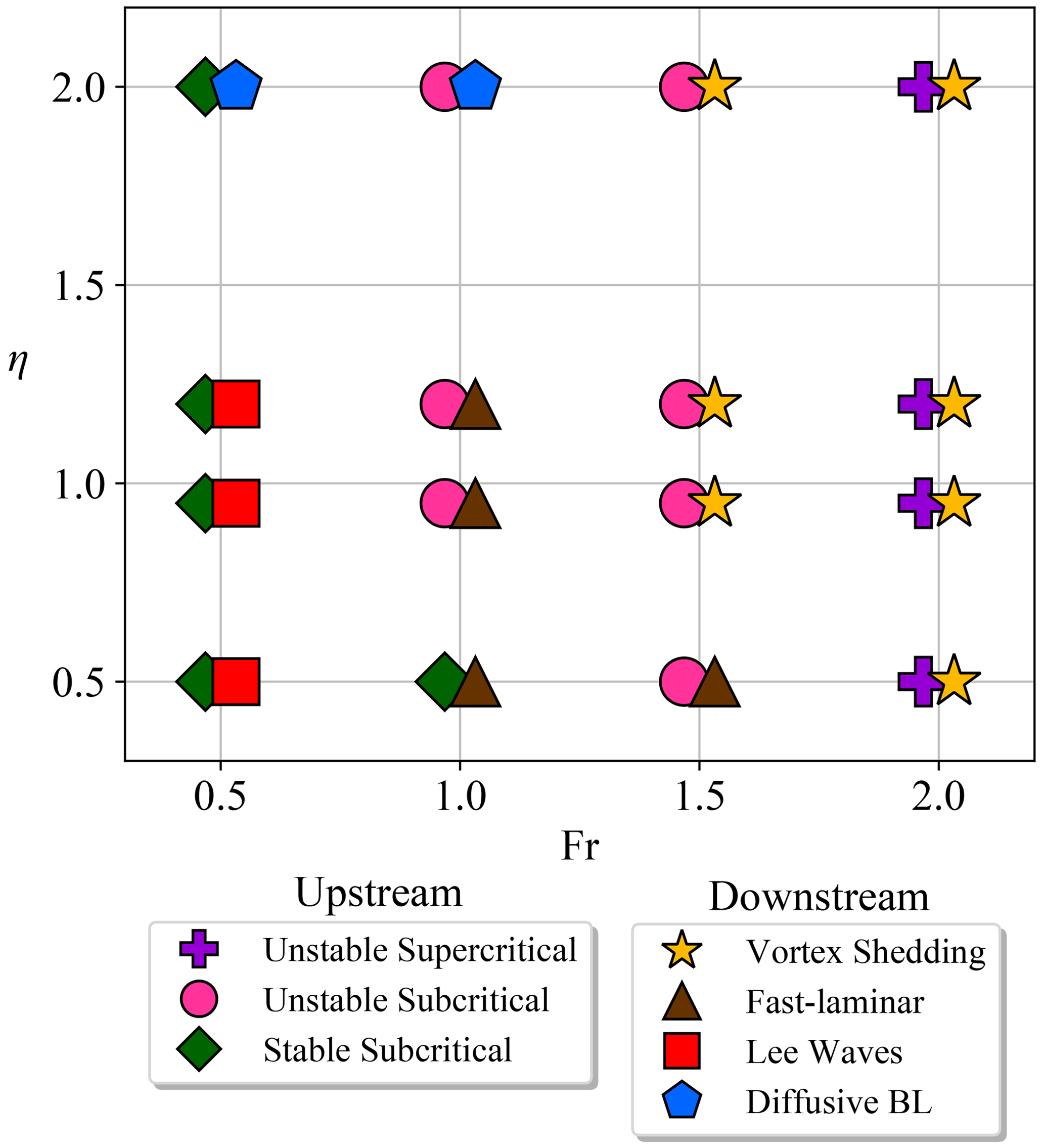
Figure 2Upstream and downstream regime classification for each simulation in dimensionless parameter space (Fr,η). The upstream and downstream markers are offset to the left and right, respectively, on the Fr axis for legibility.
3.1 Upstream regimes
In the upstream region, we identify three flow regimes: “unstable supercritical”, “unstable subcritical”, and “stable subcritical”. Figure 3 shows one representative snapshot of a set of streamlines, superposed on the density field upstream, for each regime.
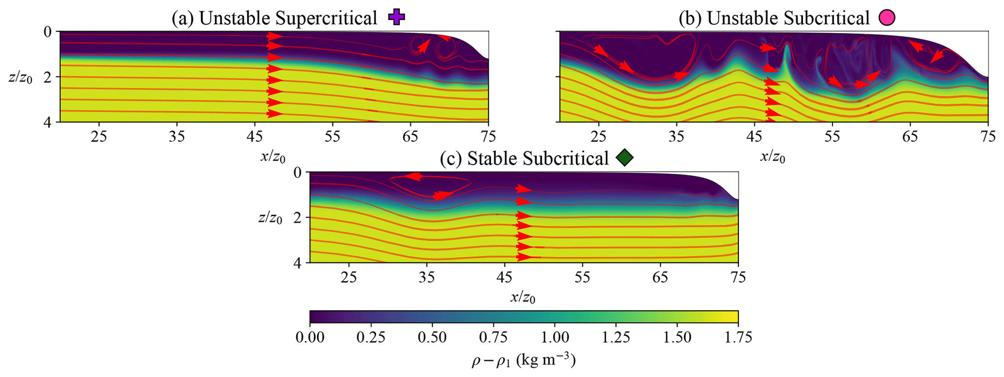
Figure 3Representative snapshots of the three upstream flow regimes' density field ρ overlaid with velocity streamlines. Each regime is assigned a marker in the title of the panel that will be used in the figures for the remainder of the paper. (a) unstable supercritical snapshot with F20H12 at t=246t0, (b) unstable subcritical with F10H20 at t=107t0, and (c) stable subcritical with F05H12 at t=90t0.
Although the subcritical and supercritical qualifiers usually relate to the local Froude number (recall Sect. 2.2), we do not measure it. Instead, we visually identify simulations where we observe upstream propagation of disturbances away from the keel and call them “subcritical” and call the others “supercritical”. This may lead to marginal disagreements with a stricter local Froude-based categorization. Indeed, the upstream disturbances we observe are sometimes nonlinear, solitary-looking waves that might propagate slightly faster than the linear propagation speed (Helfrich and Melville, 2006), the latter being part of the Froude number's definition. It is therefore possible, in principle, to see nonlinear disturbances propagate upstream in a supercritical flow. We choose to ignore these subtle theoretical considerations and base our classification on whether we can visually identify upstream wave propagation.
The qualifiers “stable” and “unstable” indicate whether small perturbations upstream of the keel eventually develop into a vigorous vorticity field, which can then cause significant stirring. We will not try to characterize or identify the instability at play, nor do we even claim that there is a single instability. When instabilities arise, they often grow from the boundary layer in contact with the keel, and their onset often coincides with the passage of the pilot light mentioned in Sect. 2.1. We find the pilot light useful in probing the stability of the flow to perturbations. Note that in some low-Fr cases, we stop the simulation before the pilot light has had time to reach the keel. In those cases, however, it dissipates very early without triggering any instability. Regardless of their origin, disturbances often amplify when they coincide with large-scale pycnocline oscillations, as seen in the relevant “Video supplement” videos. For the purposes of this work, we simply notice when vorticity grows enough to vigorously stir the flow, and we name our regimes accordingly.
The unstable supercritical regime (Figs. 3a and 4) only occurs in simulations with Fr=2.0, our largest value for this parameter. Away from the keel, we do not observe noticeable stirring of the interface. Upstream of the keel, the viscous boundary layer generates vorticity that eventually travels under the keel and downstream, as the vortices in Fig. 4b are about to do. We note that a vigorous vorticity field does not always equate to mix-inducing stirring, since the vortices in this figure mostly stir mixed-layer fluid and leave the pycnocline smooth.

Figure 4Spanwise upstream vorticity q at (a) t=187t0 and (b) t=246t0 for the F20H12 simulation in the unstable supercritical regime. The solid black line is the contour, which marks the center of the pycnocline.
The unstable subcritical regime (Figs. 3b and 5) occurs for Fr=1.5 and for all but one of the simulations with Fr=1.0. Recall that Fr is merely a bulk estimate of the local Froude numbers and does not indicate supercritical flow. In this regime, we see large-scale pycnocline oscillations that sometimes resemble solitary waves and sometimes are more turbulent, with Fig. 3b showing a hybrid example. These disturbances correlate with significant vorticity generation upstream of the keel, as evidenced by the streamlines in Fig. 3b and by the spanwise vorticity field in Fig. 5b, in the region . In the wake of these pycnocline oscillations, significant small-scale flows stir the fluid and sometimes entrain water from the deeper ocean into the mixed layer, which induces mixing (Fig. 5b at ). The mean flow then sweeps these vortices downstream towards the keel, some lasting long enough to pass under it.
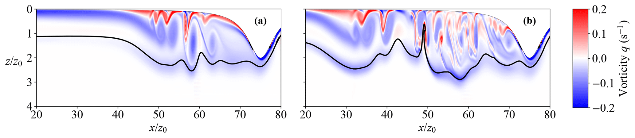
Figure 5Spanwise upstream vorticity q at (a) t=71t0 and (b) t=107t0 for the F10H20 simulation in the unstable subcritical regime. The solid black line is the contour, which marks the center of the pycnocline.
The stable subcritical regime (Fig. 3c) occurs in all simulations with Fr=0.5 and in F10H05. In this regime, we observe upstream-propagating large-scale perturbations that resemble solitary waves in F05H09 and F05H12 and appear more linear in nature in F05H05 and F10H05. In any case, the flow remains stable to perturbations, and this regime does not see much stirring.
3.2 Downstream regimes
In the downstream portion of the domain, we identify four flow regimes: “vortex shedding”, “diffusive boundary layer” “fast-laminar”, and “lee waves”. Figure 6 shows one representative snapshot per regime.
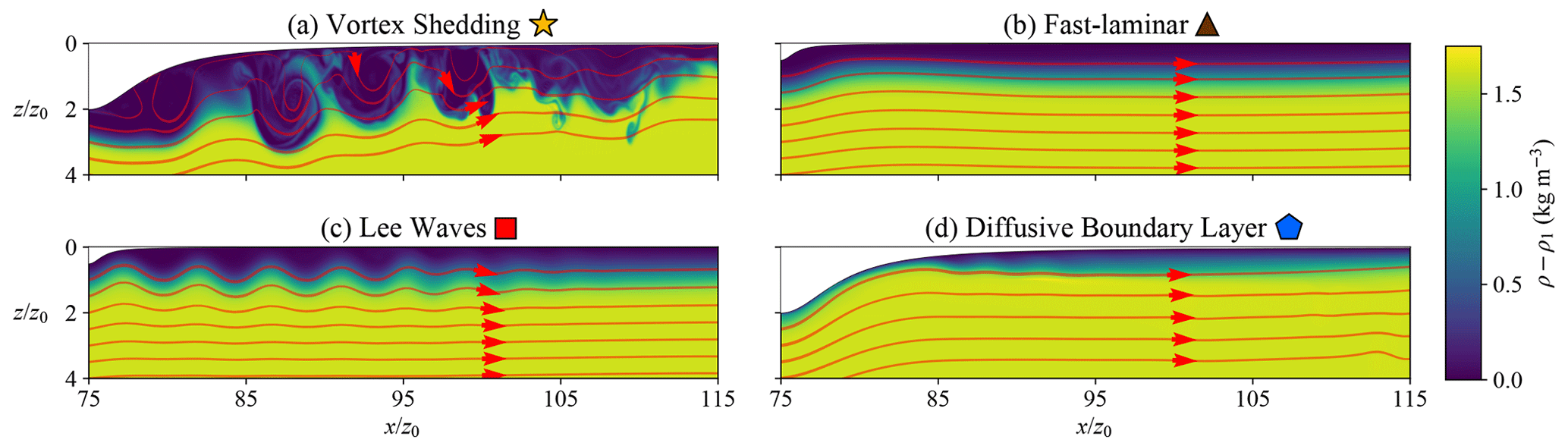
Figure 6Representative snapshots of the four downstream flow regimes' density field ρ overlaid with velocity streamlines. Each regime is assigned a marker in the title of the panel, which will be referenced in the remainder of the paper. (a) Vortex shedding corresponds to F20H20 at t=192t0, (b) fast-laminar to F10H05 at t=144t0, (c) lee waves to F05H05 at t=108t0, and (d) diffusive boundary layer to F05H20 at t=96t0.
The vortex shedding regime (Fig. 6a) is only associated with unstable upstream stirring regimes. Specifically, this regime occurs in all Fr=2.0 simulations, which we identified as unstable supercritical in the upstream region, and in simulations with Fr=1.5 and η≥0.95, which we identified as unstable subcritical simulations with the largest Froude numbers. Here, vortices downstream of the keel, the largest of which have length scales similar to the draft of the keel h, stir deeper-ocean water into the mixed layer while maintaining large local density gradients. Some vortices grow on the lee side of the keel and some originate from the upstream region (see Sect. 3.1, Figs. 4b and 5b). This regime shows phenomena that are the most closely related to turbulent hydraulic jumps.
We note that Baines (1984) did not observe what we call vortex shedding for Fr∼2. Instead, their flow remained supercritical downstream, with no noticeable vortices. However, Hester et al. (2021) did observe vortex shedding in their numerical simulations along the bottom crest of their rectangular obstacle due to flow separation at the windward edge of the obstacle (see their Fig. 7). As mentioned in Sect. 2.1, our code is based on that of Hester et al. (2021), so it is not surprising that we see similar flow behavior.
The fast-laminar regime (e.g., Fig. 6b) occurs in F15H05 and for all values of Fr=1.0 except F10H20. Most of the stirring in this regime occurs when episodic vortices generated upstream are advected under the keel (see, e.g., video for F15H05 at t≈190t0).
The lee wave regime occurs for small to moderate keel drafts, which do not completely block the mixed layer, and for the smallest Froude number (Fr=0.5). For example, in Fig. 6c, we observe a train of lee waves that extends ∼30z0 in the horizontal direction. Because the flow is slow, the creation of boundary layer vorticity is weak, and perturbations of upstream disturbances, if they pass the keel at all, do not get amplified. Therefore, stirring remains very weak.
Lastly, the defining feature of the diffusive boundary layer regime is a stream of mixed-layer water creeping along the lee side of the keel, visible for in Fig. 6d. We observe this regime when the keel draft is maximum and the Froude number is low, namely in F05H20 and F10H20. Here, we depart slightly from the purely kinematic criteria that we have applied so far to define all other regimes. Indeed, while this regime may not look visually very different from the weak stirring seen in the fast-laminar and lee-wave regimes, we will see in Sect. 4 that the mixing induced by the flow warrants its own category.
We now examine the distribution of diapycnal mixing (, , , and ) and their typical mixing depths ( and ) in all simulations, as summarized in Table 2. In the following, we use our stirring regime categorization to (1) interpret variations across simulations and (2) interpret differences between simulations that are not consistent with the null hypothesis that simulations with faster (larger Fr) and deeper (larger η) keels facilitate more diapycnal mixing (larger K, Φ) that extends over a larger depth range (larger Z).
Table 2Upstream and downstream normalized irreversible mixing rates, diapycnal diffusivities, and mixing-depth values for each simulation. is our reference value (indicated as “REF” in the table).
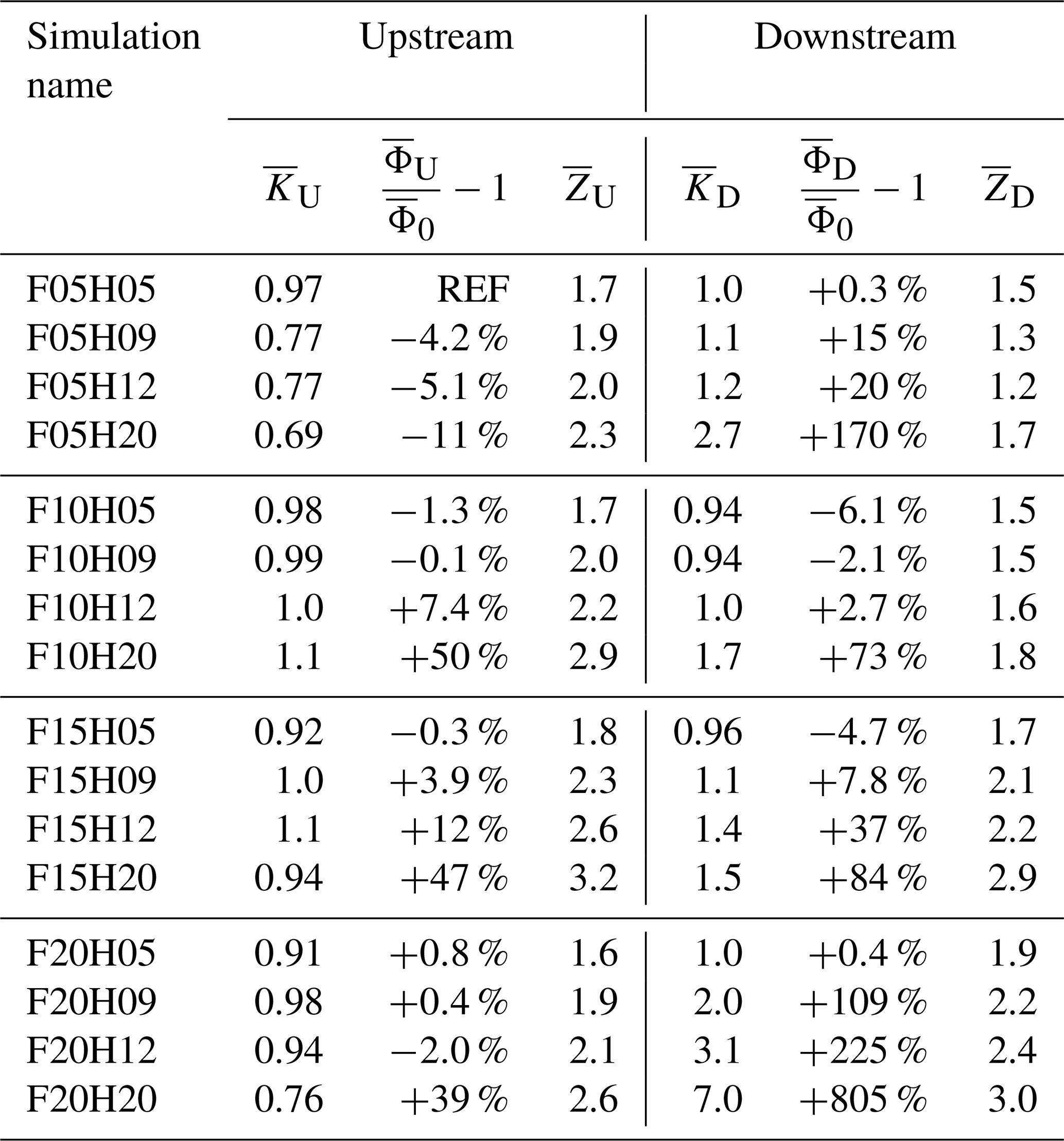
Figure 7 shows the irreversible mixing rates and for each simulation. Note that () follows trends similar to those of (), as can be pieced together from Table 2. To keep the presentation simple, we therefore focus our figures on and . We compare all of these values with , the value of in F05H05, whose flow is least disturbed by the keel of all experiments. This does not imply that is the smallest value of all the mixing rates we measure, as we are about to see.

Figure 7Time-averaged non-dimensional diapycnal mixing rate (a) upstream and (b) downstream for each simulation. For F20H20, .
Overall, upstream of the keel, we find fairly similar mixing rates across the simulations; 11 of the 16 simulations have values of that differ from by less than 10 %. We obtain comparably small mixing values possibly because the density gradient at the pycnocline is too large to allow the growth of instabilities within the pycnocline that would be required to mix it, and such instabilities are indeed not observed upstream of the keel in most simulations. This point will be discussed in further detail in Sect. 5. The remaining five simulations have the deepest keels (η=2.0), except F15H12, and differ by up to 50 % relative to . We note that the largest upstream mixing rate does not coincide with the deepest and fastest keel.
For a given Fr, simulations tend to belong to the same stirring regime that we identified in Sect. 3. Mixing rates increase with η as per our null hypothesis for Fr=1.0 and 1.5 (unstable subcritical regime) but not for Fr=0.5 (stable subcritical regime) or Fr=2.0 (unstable supercritical regime). At a given η across Fr, we find that trends in largely do not satisfy our null hypothesis, except for the unstable subcritical regime. These findings are described in greater detail below.
First, we find two instances where simulations with faster keels have less mixing than simulations with slower keels. Specifically, Fr=2.0 simulations with deeper keels (F20H12 and F20H20) have values 6 %–12 % smaller than their Fr=1.5 and Fr=1.0 counterparts (F10H12, F10H20, F15H12, and F15H20). This occurs because vortices tend to remain trapped against the keel in the thicker mixed layer that develops in simulations with deeper keels. Figure 4 shows a typical configuration for one unstable supercritical simulation (Fr=2.0), where the vortices remain close to the keel, primarily stirring the already-mixed fluid, and get swept under the keel before causing much mixing in the upstream region. Sometimes deeper vortices that extend into the deeper-ocean layer do develop and cause turbulent mixing but occur rather infrequently, leading to an insignificant contribution to the average mixing rates.
In contrast, the deeper keel simulations with smaller Fr=1.0 and 1.5 have larger vortices that occur more frequently, are able to sometimes pull deep water into the upper layer (see, e.g., Figs. 3b and 5b around taken from F10H20), and remain in the upstream region longer (consistent with the subcritical flow categorization), which induces more mixing upstream. In particular, Fig. 3b shows an example of the stronger density gradients that are induced by perturbations in the interface in these simulations in the unstable subcritical regime. These density perturbations get larger with both η and Fr, resulting in trends in that are consistent with our null hypothesis.
Second, considering only simulations with Fr=0.5 (stable subcritical regime), we find that simulations with deeper keels have less mixing than those with shallower keels. For example, the simulation with the shallowest keel (F05H05) has a value 11 % larger than the simulation with the deepest keel (F05H20). Although we did not investigate this result in detail, visual inspection of the videos suggests that this is caused by the tendency for deep keels to block more flow. The blocked flow causes the distance between two isopycnals in the upstream stagnant layer to increase, implying smaller density gradients and less mixing.
Overall, downstream of the keel, we find more variation between simulations than upstream of the keel, with only 7 out of 16 simulations yielding mixing rates that differ by less than 10 % from . Of the remaining nine simulations, six have rates that are at least 73 % larger than , and three simulations have . We note that these three simulations are in the downstream vortex shedding and upstream unstable supercritical regimes, implying that all vortices formed upstream are pushed downstream. Notably, the vortex shedding events are episodic. As such, for F20H05, in which only one vortex shedding event occurs over our averaging time interval, . During the event, mixing is enhanced with rates up to .
For a given Fr, we find that deeper keels do indeed mix more and therefore satisfy the null hypothesis. Furthermore, when Fr≥1.0, faster keels (increasing Fr) mix more for a given keel height η, also in line with the null hypothesis. On the other hand, there are several instances where simulations with faster keels have less mixing than those with slower keels. Specifically, for a given η, decreases when Fr increases from 0.5 to 1.0. Based on our stirring regime categorization, this appears to occur for either of two reasons: first, for η≤1.2, in the lee wave regime of the Fr=0.5 simulations (F05H05, F05H10, and F05H12), the isopycnals are spatially perturbed, resulting in larger density gradients and greater mixing than in the fast-laminar regime (Fr=1.0), where isopycnals are predominantly flat (cf. Fig. 6b and c). In the fast-laminar regime, mixing is episodically enhanced by passing vortices that are generated and advected from the upstream, but these isopycnal perturbations and thus induced mixing are small at Fr=1.0. Second, the F05H20 to F10H20 transition at η=2.0, which occurs in the diffusive boundary layer regime, also sees a drop in . In this regime, most of the mixing happens in the diffusive boundary layer against the lee side of the keel. This boundary layer is much thinner in F05H20 than in the faster flowing F10H20, whereas the buoyancy difference ΔB across both boundary layers is always the same. The net result, after spatial integration, is more mixing in F05H20 than in F10H20. We leave a more quantitative analysis of these deviations to future studies.
In addition to the variability in mixing rates, we are also interested in the mixing depth, i.e., how deep mixing penetrates relative to the pycnocline depth depending on keel height and speed. Figure 8 displays and for each experiment. Recall from Sect. 2.3 that ZΩ, with Ω=U or D, is the depth that captures 95 % of the integrand of ΦΩ in Eq. (12) and therefore provides an estimate of how deep we see active mixing. On average, we find that vertical mixing extends approximately twice as deep as the initial depth of the mixed layer, both upstream and downstream. Specifically, we find that upstream , with an average ± 0.5, and downstream , with an average ± 0.5 (where ± indicates 1 standard deviation).
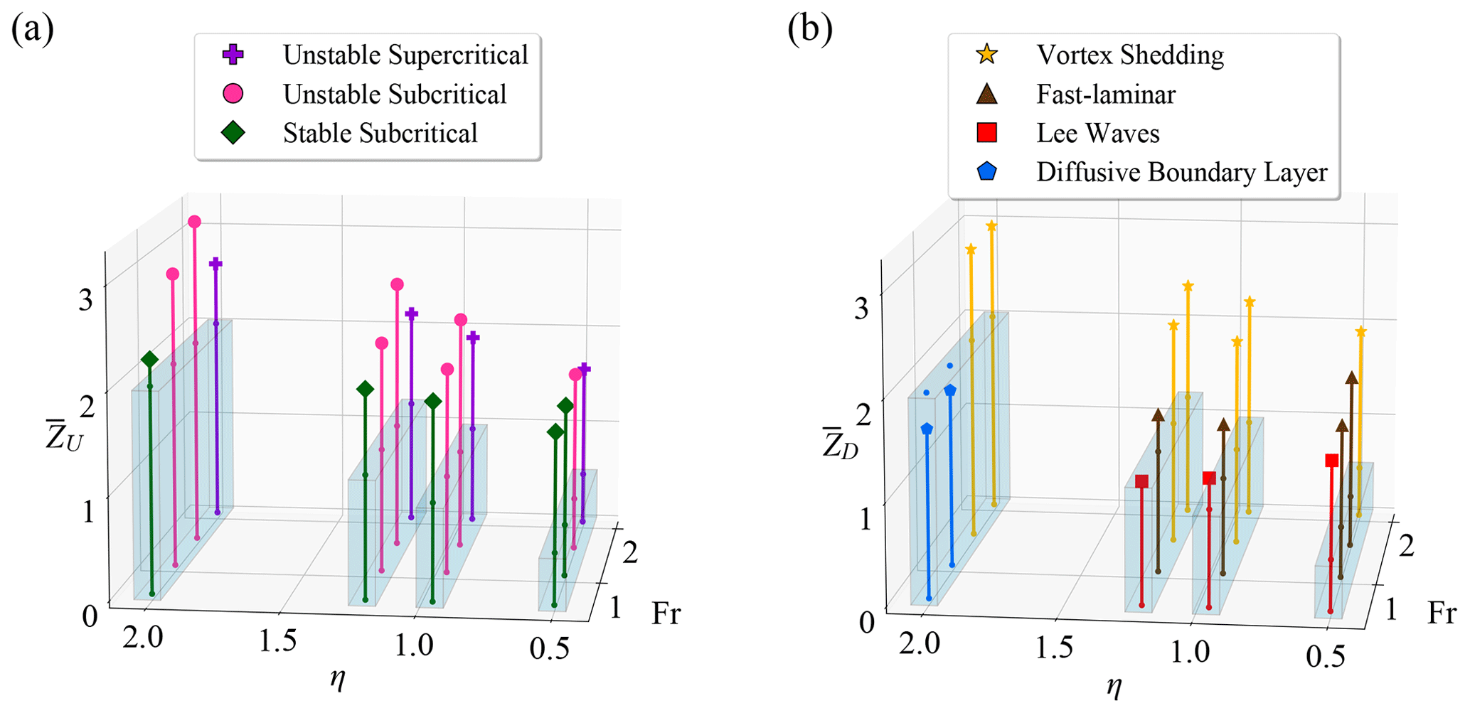
Figure 8(a) and (b) for each simulation. The translucent rectangular boxes mark the non-dimensional keel drafts η, and the small round markers mark the depths z=0 and . As a reminder, implies a mixing depth equal to the mixed-layer depth.
For most simulations, in the upstream and downstream, we find that the mixing depth increases both with keel speed (larger Fr) and keel height (larger η). However, the comparison of the upstream mixing depth values in the simulations with Fr=2.0 to Fr=1.5 indicates that flows induced by faster keels of the same height can result in mixing that occurs over a shallower depth range. This possibly occurs because Fr=1.5 simulations have a subcritical flow and, therefore, can trap vortices upstream, which can ultimately deepen the range of mixing. In contrast, Fr=2.0 simulations have a supercritical flow, and vortices, which could otherwise increase , are swept downstream. Indeed, downstream of the keel, where such vortices enhance mixing, mixing depth is larger in simulations with Fr=2.0 than in those with Fr=1.5.
We find that, in almost all the simulations, mixing extends below the keel both upstream and downstream (i.e., , ), with the exceptions of the downstream mixing in F05H20 and F10H20. These two simulations are described downstream by the diffusive boundary layer regime, in which mixing predominantly occurs along the lee-side boundary of the keel. This result, along with the trend in mixing rate that is contrary to our null hypothesis for these two simulations (Fig. 7b), supports our classification of these simulations in their own distinct regime, even though their streamlines resemble those of the fast-laminar regime (see Fig. 6).
We caution against overinterpreting these numbers. Indeed, the differences between them are often smaller than the standard deviation of the mixing depth for a given simulation over the time average. In addition, our pycnocline is on the thinner side (∼0.5z0 after settling) in comparison to other seasonal pycnocline measurements (thickness values beyond z0 are possible, as seen in PFW). Simulations with large mixing rates due to entrainment of the deeper ocean ( or , as in the vortex shedding regime) would likely see reduced rates for a thicker pycnocline.
5.1 Implications for a changing Arctic Ocean
We have presented results examining how the size and speed of an ice keel impacts ocean mixing using idealized simulations with different ice keel characteristics (different values of η and Fr). To put our findings in context, we used observations reported by previous studies to roughly estimate climatological averages and decadal trends of η and Fr in the Arctic Ocean. Specifically, we select climatological averages and decadal trends of U, h, ΔB, and z0 to estimate climatological values and decadal trends of η and Fr. The majority of our parameter estimates are derived from 30-year surface wind and mixed-layer properties documented by PFW. These values are estimated using data collected between 1979–2012 for five separate Arctic regions: Chukchi Sea, southern Beaufort Sea, Canada Basin, Eurasian Basin, and Barents Sea. We therefore provide climatological and trend estimates of η and Fr for each of these regions. Details on our choice for each parameter are given below.
We estimate the summer mixed-layer depth (z0) and the buoyancy difference between the mixed layer and deeper ocean (ΔB) using mixed-layer properties reported by PFW, where we set deeper-ocean-layer properties equal to observed winter mixed-layer properties. This is similar to PFW, who also considered a two-layer ocean associated with summer and winter mixed-layer properties to examine variations in the seasonal pycnocline. Specifically, we use their reported below-ice mixed-layer depth and salinity climatological averages in April and July (see their Figs. 6 and 8) for the winter and summer mixed layers, respectively, to estimate averages in z0 and ΔB. For our trends in z0 and ΔB, we use their below-ice summer mixed-layer depth and salinity trends that ranged from −3.9 to +3.3 m per decade and −1.9 to +2.9 psu per decade, respectively, depending on the region (see their Fig. 14). Trends in regions that are reported to be insignificant by PFW were taken to have no trend.
We use a climatological pan-Arctic ice speed U=0.2 m s−1, consistent with measurements of ice speeds collected in both the 1970s (McPhee and Smith, 1976) and the 2000s (Cole et al., 2017). This is a vast simplification, as in reality U varies largely across the Arctic due to spatial and temporal variability in wind forcing and semidiurnal tides. For each Arctic region, we estimate the decadal trend in ice velocity using 30-year regional near-surface wind trends reported by PFW and applying the “rule of thumb” introduced by Thorndike and Colony (1982), which approximates the ice speed by 2 % of the surface wind speed. With this approach, we estimate ice-speed trends as large as +3.2 cm s−1 per decade, depending on the region (with some regions indicating no trend).
Lastly, lacking data for climatological or decadal trends of ice keel drafts (h), we instead repeat our analysis using two different keel sizes. That is to say that for each region, we compute η twice: first setting h=7.45 m, the average keel draft reported by Wadhams (2012) and Kvadsheim (2014), and second using h=18.6 m, which is chosen to examine the same range of η that we were able to examine in our simulations.
Figure 9 shows the resulting climatological averages (numbered boxes) and 5- or 15-year estimates (solid or dashed arrows, respectively) of η and Fr for 10 scenarios: one for each of the five Arctic regions using one of two keel sizes: 7.45 m (orange) and 18.6 m (cyan). The 5-year estimates were chosen for some regions (Chukchi Sea and southern Beaufort Sea) because their two-layer stratifications become unstable (summer mixed layer becomes saltier than winter mixed layer) after some number of years (e.g., southern Beaufort Sea after 7.5 years) due to their salinity decadal trends.

Figure 9Upstream and downstream regime classifications for each regime in dimensionless parameter space (Fr,η) (Fig. 2) overlaid with range estimates of five Arctic regions: Chukchi Sea (1), southern Beaufort Sea (2), Canada Basin (3), Eurasian Basin (4), and Barents Sea (5). The simulation regime markers are scaled by their respective mixing rates. The orange and cyan square markers indicate climatological average (Fr,η) values for the 7.45 and 18.6 m keels, respectively. The transparent boxes indicate 1 standard deviation range in Fr and η. The arrow for each marker points to where the average will be in 5 years (solid) or 15 years (dashed) based on observed 30-year trends. Note that for the 18.6 m keel (cyan), the Canada Basin (3) is predicted to reach (0.87,4.72). Markers with (*) indicate that a mixed-layer or wind speed trend was reportedly insignificant.
On average, we find that each scenario has , where differences in ice keel size explain most of the variation in η (as expected by our choice of keel sizes; see above). These ranges roughly double after considering approximately 68 % of the variability (indicated by cyan and orange shadings). Our trend estimates indicate that Fr is increasing for each scenario, with the largest positive trend in the southern Beaufort Sea (+0.62 per decade) and the smallest increase in the Barents Sea (+0.039 per decade). In contrast, we find both positive and negative trends for η, depending on the region. We estimate for the 7.45 m (18.6 m) keel that η is decreasing at a rate of 0.29 (0.71) per decade in the southern Beaufort Sea, increasing at a rate of 0.70 (1.8) and 0.032 (0.08) per decade in the Canada and Eurasian basins, respectively, and does not change in the Chukchi and Barents seas due to insignificant trends in the mixed-layer depth.
Next, we consider the climatological averages together with the results from our simulations (based on where cyan and orange shadings overlap with colored shapes; Fig. 9). For scenarios with large ice keels (h=18.6 m; cyan shadings), we find that all stirring regimes are expected to occur except the unstable supercritical upstream regime. These simulations were associated with mixing that could vary by up to 50 % upstream and 170 % downstream of the background mixing rate (Table 2). By contrast, scenarios with smaller ice keels (h=7.45 m; orange shadings) span a smaller range of Fr–η space and are only expected to be associated with the subcritical upstream stirring regimes and the lee wave and fast-laminar downstream stirring regimes. These simulations were associated with mixing that only varied up to 10 % upstream and 20 % downstream of the background mixing rate. Again, we caution against over-interpreting these numbers (see below for more on this point). Finally, the estimated trends in Fr- and η-associated observed decadal changes to ice speeds and upper-ocean properties (arrows) suggest that all stirring regimes and associated variations in mixing across our entire suite of simulations could be relevant below a changing Arctic ice cover. This suggests that more robust observational estimates, particularly of ice keel sizes and speeds, will be necessary to properly estimate current and future below-ice mixing.
5.2 Limitations
To our knowledge, we have presented the first set of idealized experiments specifically aimed at examining how ice keel size and speed impacts ocean mixing. While our findings are novel, we emphasize that this work is an initial step in examining this problem and that more realistic simulations will be necessary to properly parameterize ice-keel-driven mixing in coupled models. We expand on the limitations of our current setup in the following.
First, we choose large values of viscosity and diffusivity to ensure numerical stability, but these choices have further consequences in addition to a strong stratification from our two-layer model. Mainly, they reduce the buoyancy Reynolds number Reb, which can be thought of as the ratio of the strength of turbulent instabilities that can induce vertical mixing to the combined strength of stratification and viscosity that impedes vertical motions and mixing. The buoyancy Reynolds number has been shown to control diffusivity and diapycnal mixing rates (Shih et al., 2005; Mashayek et al., 2017). In particular, for small Reb (i.e., weak turbulent flows and/or large stratification and viscosity) as in our simulations, mixing rates and diffusivity tend to be small because turbulence-induced instabilities are not strong enough to overcome stabilizing effects (Bouffard and Boegman, 2013; Salehipour and Peltier, 2015). In other words, our mixing instead tends to happen through laminar diffusion of buoyancy across smooth density gradients, whereas in a more realistic fluid with larger Reb, such mixing would happen through episodes of small-scale turbulence in the pycnocline or more widely observed turbulent hydraulic jumps downstream (see, e.g., Winters and Armi, 2012; Lawrence and Armi, 2022). Our upstream unstable subcritical and downstream vortex shedding regimes feature such mixing events, which we may have observed more generally had we been able to use a finer resolution and smaller values of μ. We leave it to future studies to investigate how smaller viscosity and enhanced turbulence translate into quantitative differences for , , , and .
Second, our simulations use a two-dimensional domain to model what is a three-dimensional process in the ocean. Since keels can extend 100 m in the transverse direction (Topham et al., 1988), we can consider that our simulations are qualitatively representative of the flow in wide keels' cross-sections far away from their lateral ends. Note that, by assuming that there are no ridges or irregularities on the keel, we ignore additional generators of small-scale turbulence, and thus of stirring. This may result in underestimating mixing. However, our enhanced viscosity yields a thick viscous boundary layer, which may compensate (in full or in part) for the absence of ice roughness. In addition, ice keels are conglomerates of ice rubble with varying degrees of porosity. As such, our no-slip condition at the keel boundary is not necessarily realistic, particularly for young keels. Accounting for porous flow would require a more intricate model, which is left for future work.
Third, because our simulations are two-dimensional, the turbulence we see sometimes follows an inverse cascade of energy, especially for vortices entirely contained in either the mixed or the deeper-ocean layer. That is to say that instead of twisting and stretching into smaller and smaller structures, vortices of the same sign merge and become larger and larger in diameter (Vallis, 2017). This process could contribute to artificially expanding the diameters of the vortices we see in the upstream unstable sub- and supercritical regimes and the downstream vortex shedding regime, which cause the largest values of and as well as the deepest mixing depths and . As a first consequence, we might be overestimating some values for our mixing depth. As for and , the inverse cascade may have two separate effects. First, the large size of the vortices in the mixed layer might lead to more entrainment of deep fluid into the mixed layer, enhancing local density gradients and therefore turbulent mixing. On the other hand, mixing in stratified flows occurs through a host of secondary instabilities that are three-dimensional in nature (e.g., Mashayek and Peltier, 2012a, b). Such instabilities are absent from our two-dimensional simulations, which is likely to have qualitative and quantitative consequences on the values of effective diffusivities.
Fourth, in the Arctic Ocean, there are roughly 2.0 to 4.5 keels per kilometer (Wadhams, 1981), which roughly translates to a keel every 28z0 to 63z0. Although we do not account for additional keels in our domain, any fluid phenomena such as vortices, solitary waves, and lee waves develop within 25z0 of the keel. This means that our flow regimes in theory have enough space to realistically form in the Arctic Ocean and could be representative of the dynamics underneath an entire floe with one keel (ignoring the floe's edges). However, the establishment of these flow regimes assumes an upstream and downstream flow similar to the initial conditions that are not affected by surrounding keels. An additional keel present upstream would mix (to varying degrees) the established pycnocline, smoothing the two-layer stratification of the incident current, thus changing the dynamics of the situation. Furthermore, an additional keel downstream from the keel of interest in the subcritical unstable regime could generate upstream-propagating internal waves and would further complicate the problem.
Fifth, fixing the temperature of our domain at the freezing point of seawater necessarily suppresses melting of the keel. Aside from structurally changing the keel, melting would produce a stabilizing buoyancy flux of freshwater immediately below the ice that could hinder turbulence and, consequently, mixing. The rate of melting responds to the keel's ability to draw up heat fluxes from below and to mix or stir away the fresh meltwater immediately below the ice (Skyllingstad et al., 2003). For instance, regimes like vortex shedding would likely see high melting rates because of their large mixing rates and mixing depths; however, the effects of the stabilizing buoyancy flux from the subsequent meltwater on the regime's mixing rates are uncertain and require further work. If our ice keel speed were physically variable (i.e., influenced by drag), then melting could hydrodynamically “decouple” the ice floe and its keel(s) from the upper ocean boundary layer, reducing drag and allowing the floe to travel faster; however, this is beyond the scope of this paper. The reader is referred to McPhee (2012) for more information.
With these considerations in mind, we caution the reader against directly comparing our numbers and simulated processes with measurements made in the Arctic Ocean. However, by comparing the same metrics across the simulations, the regimes and parameters we defined should provide useful qualitative guidance as to which real-world situation might lead to more or less mixing than another.
We performed 16 numerical simulations of two-layer fluid flow over the cross-section of an ice keel (Fig. 1), targeted at understanding how mixing varies for the bulk Froude number Fr and relative keel draft η. We estimated that the Arctic Ocean should exhibit a range of non-dimensional ice keel speeds of and non-dimensional ice keel depths of . We were able to explore approximately half of this parameter space ( and ) and found within this domain a fairly broad range of dynamics. Specifically, we characterized the variety of flows that were generated from flow across the ice keel using three upstream and four downstream stirring regimes (Figs. 2, 3, and 6). Further, we found that these dynamics were essential for explaining differences in mixing across simulations (Figs. 7 and 8).
What do these results mean for accurately representing ice keel mixing below a rapidly changing sea ice cover in coupled models? The range of mixing levels across simulations further supports previous studies that found that ice–ocean momentum exchange is sensitive to factors aside from wind speed. The majority of these studies suggested that changing ice keel sizes should be considered because larger ice keels can increase ice–ocean drag. Our results have added another level of complexity to this paradigm by demonstrating that, in contrast to ice–ocean drag, ocean mixing does not increase monotonically with larger keel depth and speed. Instead, our simulations demonstrate that larger, faster ice keels can substantially inhibit or enhance ocean mixing and that this depends on the generation and propagation of vortices and turbulence. Finally, our results highlight that improved estimates of current and future below-ice mixing will require two key pieces of information: (1) better observational estimates of ice keel characteristics and (2) more realistic numerical simulations aimed at examining how the size and speed of ice keels impact ocean mixing.
The simulation and processing code as well as the calculations used to create Fig. 9 can be found at https://doi.org/10.5281/zenodo.8170312 (De Abreu et al., 2023a).
Simulation output can be found at https://doi.org/10.5281/zenodo.12627827 (De Abreu et al., 2024).
Videos of all 16 simulations can be found at https://doi.org/10.5281/zenodo.8169338 (De Abreu et al., 2023b).
RMC developed the simulation code with guidance from MGS. SDA made significant modifications to the simulation code. VEZ and SDA created the simulation post-processing code for the mixing analysis. SDA ran the simulations with the post-analysis performed by everyone. The paper was primarily written by SDA, ER and, NG with the figures created by SDA and RMC. Everyone edited and revised the paper for submission.
The contact author has declared that none of the authors has any competing interests.
Publisher's note: Copernicus Publications remains neutral with regard to jurisdictional claims made in the text, published maps, institutional affiliations, or any other geographical representation in this paper. While Copernicus Publications makes every effort to include appropriate place names, the final responsibility lies with the authors.
Sam De Abreu, Rosalie M. Cormier, Mikhail G. Schee, and Nicolas Grisouard acknowledge the support of Natural Sciences and Engineering Research Council of Canada (NSERC). Sam De Abreu was supported by ArcticNet from the Networks of Centres of Excellence Canada (project 52551). Varvara E. Zemskova acknowledges the support of the National Science Foundation. Erica Rosenblum was supported by the NSERC PDF award, the NSERC Canada-150 Chair, and the NSERC Discovery Grant. Erica Rosenblum is grateful to the researchers, staff, and students of the Centre for Earth Observation Science for support received during preparation of this paper. Computations were performed on the Niagara supercomputer at the SciNet HPC Consortium (Loken et al., 2010; Ponce et al., 2019). SciNet is funded by the Canada Foundation for Innovation; the Government of Ontario; Ontario Research Fund – Research Excellence; and the University of Toronto. We thank Ilker Fer and another anonymous referee for their constructive comments.
This research has been supported by the Natural Sciences and Engineering Research Council of Canada (grant nos. RGPIN-2015-03684, RGPIN-2022-04560, G00321321, and RGPIN-2024-05545) and National Science Foundation (grant nos. OCE1756752, OCE2220439).
This paper was edited by Jari Haapala and reviewed by Ilker Fer and one anonymous referee.
Baines, P. G.: A unified description of two-layer flow over topography, J. Fluid Mech., 146, 127–167, https://doi.org/10.1017/S0022112084001798, 1984. a, b, c, d
Barthélemy, A., Fichefet, T., Goosse, H., and Madec, G.: Modeling the interplay between sea ice formation and the oceanic mixed layer: Limitations of simple brine rejection parameterizations, Ocean Model., 86, 141–152, https://doi.org/10.1016/j.ocemod.2014.12.009, 2015. a
Bouffard, D. and Boegman, L.: A diapycnal diffusivity model for stratified environmental flows, Dynam. Atmos. Oceans, 61–62, 14–34, https://doi.org/10.1016/j.dynatmoce.2013.02.002, 2013. a
Brenner, S., Rainville, L., Thomson, J., Cole, S., and Lee, C.: Comparing Observations and Parameterizations of Ice-Ocean Drag Through an Annual Cycle Across the Beaufort Sea, J. Geophys. Res.-Oceans, 126, e2020JC016977, https://doi.org/10.1029/2020JC016977, 2021. a
Brown, K. A., Holding, J. M., and Carmack, E. C.: Understanding Regional and Seasonal Variability Is Key to Gaining a Pan-Arctic Perspective on Arctic Ocean Freshening, Frontiers in Marine Science, 7, 1–25, https://doi.org/10.3389/fmars.2020.00606, 2020. a
Burns, K. J., Vasil, G. M., Oishi, J. S., Lecoanet, D., and Brown, B. P.: Dedalus: A flexible framework for numerical simulations with spectral methods, Physical Review Research, 2, 023068, https://doi.org/10.1103/PhysRevResearch.2.023068, 2020. a
Carmack, E., Polyakov, I., Padman, L., Fer, I., Hunke, E., Hutchings, J., Jackson, J., Kelley, D., Kwok, R., Layton, C., Melling, H., Perovich, D., Persson, O., Ruddick, B., Timmermans, M.-L., Toole, J., Ross, T., Vavrus, S., and Winsor, P.: Toward Quantifying the Increasing Role of Oceanic Heat in Sea Ice Loss in the New Arctic, B. Am. Meteorol. Soc., 96, 2079–2105, https://doi.org/10.1175/BAMS-D-13-00177.1, 2015. a
Carr, M., Sutherland, P., Haase, A., Evers, K., Fer, I., Jensen, A., Kalisch, H., Berntsen, J., Părău, E., Thiem, Ø., and Davies, P. A.: Laboratory Experiments on Internal Solitary Waves in Ice-Covered Waters, Geophys. Res. Lett., 46, 12230–12238, https://doi.org/10.1029/2019GL084710, 2019. a
Cole, S. T., Toole, J. M., Lele, R., Timmermans, M.-L., Gallaher, S. G., Stanton, T. P., Shaw, W. J., Hwang, B., Maksym, T., Wilkinson, J. P., Ortiz, M., Graber, H., Rainville, L., Petty, A. A., Farrel, S. L., Richter-Menge, J. A., and Haas, C.: Ice and ocean velocity in the Arctic marginal ice zone: Ice roughness and momentum transfer, Elementa, 5, 55, https://doi.org/10.1525/elementa.241, 2017. a, b, c
Cole, S. T., Toole, J. M., Rainville, L., and Lee, C. M.: Internal Waves in the Arctic: Influence of Ice Concentration, Ice Roughness, and Surface Layer Stratification, J. Geophys. Res.-Oceans, 123, 5571–5586, https://doi.org/10.1029/2018JC014096, 2018. a
Cummins, P. F.: Numerical Simulations of Upstream Bores and Solitons in a Two-Layer Flow past an Obstacle, J. Phys. Oceanogr., 25, 1504–1515, https://doi.org/10.1175/1520-0485(1995)025<1504:NSOUBA>2.0.CO;2, 1995. a
De Abreu, S., Cormier, R. M., Schee, M. G., Zemskova, V. E., Rosenblum, E., and Grisouard, N.: Two-dimensional Numerical Simulations of Mixing under Ice Keels Python Code (1.0.1), Zenodo [code], https://doi.org/10.5281/zenodo.8170312, 2023a. a
De Abreu, S., Cormier, R. M., Schee, M. G., Zemskova, V. E., Rosenblum, E., and Grisouard, N.: Two-dimensional Numerical Simulations of Mixing under Ice Keels Videos, Zenodo [video], https://doi.org/10.5281/zenodo.8169338, 2023b. a
De Abreu, S., Cormier, R. M., Schee, M. M., Zemskova, V. E., Rosenblum, E., and Grisouard, N.: Two-dimensional Numerical Simulations of Mixing under Ice Keels Data, Zenodo [data set], https://doi.org/10.5281/zenodo.12627827, 2024. a
Dosser, H. V., Chanona, M., Waterman, S., Shibley, N. C., and Timmermans, M.: Changes in Internal Wave-Driven Mixing Across the Arctic Ocean: Finescale Estimates From an 18-Year Pan-Arctic Record, Geophys. Res. Lett., 48, e2020GL091747, https://doi.org/10.1029/2020GL091747, 2021. a
Fer, I. and Sundfjord, A.: Observations of upper ocean boundary layer dynamics in the marginal ice zone, J. Geophys. Res., 112, C04012, https://doi.org/10.1029/2005JC003428, 2007. a, b
Fer, I., Baumann, T. M., Koenig, Z., Muilwijk, M., and Tippenhauer, S.: Upper-Ocean Turbulence Structure and Ocean-Ice Drag Coefficient Estimates Using an Ascending Microstructure Profiler During the MOSAiC Drift, J. Geophys. Res.-Oceans, 127, e2022JC018751, https://doi.org/10.1029/2022JC018751, 2022. a, b
Fine, E. C. and Cole, S. T.: Decadal Observations of Internal Wave Energy, Shear, and Mixing in the Western Arctic Ocean, J. Geophys. Res.-Oceans, 127, e2021JC018056, https://doi.org/10.1029/2021jc018056, 2022. a
Fofonoff, N. and Millard, R.: Algorithms for Computation of Fundamental Properties of Seawater, UNESCO Tech. Pap. Mar. Sci., 44, https://doi.org/10.25607/OBP-1450, 1983. a
Guthrie, J. D. and Morison, J. H.: Not Just Sea Ice: Other Factors Important to Near-inertial Wave Generation in the Arctic Ocean, Geophys. Res. Lett., 48, e2020GL090508, https://doi.org/10.1029/2020GL090508, 2021. a
Helfrich, K. R. and Melville, W. K.: Long Nonlinear Internal Waves, Annu. Rev. Fluid Mech., 38, 395–425, https://doi.org/10.1146/annurev.fluid.38.050304.092129, 2006. a
Hester, E. W., McConnochie, C. D., Cenedese, C., Couston, L.-A., and Vasil, G.: Aspect ratio affects iceberg melting, Physical Review Fluids, 6, 023802, https://doi.org/10.1103/PhysRevFluids.6.023802, 2021. a, b, c
Holland, D. M., Rosales, R. R., Stefanica, D., and Tabak, E. G.: Internal hydraulic jumps and mixing in two-layer flows, J. Fluid Mech., 470, 63–83, https://doi.org/10.1017/S002211200200188X, 2002. a
Holloway, G., Dupont, F., Golubeva, E., Häkkinen, S., Hunke, E., Jin, M., Karcher, M., Kauker, F., Maltrud, M., Morales Maqueda, M. A., Maslowski, W., Platov, G., Stark, D., Steele, M., Suzuki, T., Wang, J., and Zhang, J.: Water properties and circulation in Arctic Ocean models, J. Geophys. Res.-Oceans, 112, 1–18, https://doi.org/10.1029/2006JC003642, 2007. a
Houghton, D. D. and Kasahara, A.: Nonlinear shallow fluid flow over an isolated ridge, Commun. Pure Appl. Math., 21, 1–23, https://doi.org/10.1002/cpa.3160210103, 1968. a
Hutchings, J. K. and Faber, M. K.: Sea-Ice Morphology Change in the Canada Basin Summer: 2006–2015 Ship Observations Compared to Observations From the 1960s to the Early 1990s, Front. Earth Sci., 6, 2006–2015, https://doi.org/10.3389/feart.2018.00123, 2018. a, b
Ilicak, M., Drange, H., Wang, Q., Gerdes, R., Aksenov, Y., Bailey, D., Bentsen, M., Biastoch, A., Bozec, A., Böning, C., Cassou, C., Chassignet, E., Coward, A. C., Curry, B., Danabasoglu, G., Danilov, S., Fernandez, E., Fogli, P. G., Fujii, Y., Griffies, S. M., Iovino, D., Jahn, A., Jung, T., Large, W. G., Lee, C., Lique, C., Lu, J., Masina, S., George Nurser, A. J., Roth, C., Salas y Mélia, D., Samuels, B. L., Spence, P., Tsujino, H., Valcke, S., Voldoire, A., Wang, X., and Yeager, S. G.: An assessment of the Arctic Ocean in a suite of interannual CORE-II simulations. Part III: Hydrography and fluxes, Ocean Model., 100, 141–161, https://doi.org/10.1016/j.ocemod.2016.02.004, 2016. a
Jin, M., Hutchings, J., Kawaguchi, Y., and Kikuchi, T.: Ocean mixing with lead-dependent subgrid scale brine rejection parameterization in a climate model, J. Ocean U. China, 11, 473–480, https://doi.org/10.1007/s11802-012-2094-4, 2012. a
Kvadsheim, S.: Ice ridge keel size distributions, Ph.D. thesis, Norwegian University of Science and Technology, Trondheim, http://hdl.handle.net/11250/247276 (last access: 2023), 2014. a, b
Kwok, R.: Arctic sea ice thickness, volume, and multiyear ice coverage: Losses and coupled variability (1958–2018), Environ. Res. Lett., 13, 105005, https://doi.org/10.1088/1748-9326/aae3ec, 2018. a, b
Kwok, R. and Rothrock, D. A.: Decline in Arctic sea ice thickness from submarine and ICESat records: 1958–2008, Geophys. Res. Lett., 36, 1–5, https://doi.org/10.1029/2009GL039035, 2009. a
Large, W. G., McWilliams, J. C., and Doney, S. C.: Oceanic vertical mixing: A review and a model with a nonlocal boundary layer parameterization, Rev. Geophys., 32, 363, https://doi.org/10.1029/94RG01872, 1994. a
Lavoie, J., Tremblay, B., and Rosenblum, E.: Canada Basin hydrography in the CESM-LE and observations: implications for vertical ocean heat transport in a transitioning sea ice cover, ESS Open Archive, 1–34, https://doi.org/10.1002/essoar.10507467.1, 2021. a
Lawrence, G. A. and Armi, L.: Stationary internal hydraulic jumps, J. Fluid Mech., 936, A25, https://doi.org/10.1017/jfm.2022.74, 2022. a
Liang, X. and Losch, M.: On the Effects of Increased Vertical Mixing on the Arctic Ocean and Sea Ice, J. Geophys. Res.-Oceans, 123, 9266–9282, https://doi.org/10.1029/2018JC014303, 2018. a
Lincoln, B. J., Rippeth, T. P., Lenn, Y., Timmermans, M. L., Williams, W. J., and Bacon, S.: Wind-driven mixing at intermediate depths in an ice-free Arctic Ocean, Geophys. Res. Lett., 43, 9749–9756, https://doi.org/10.1002/2016GL070454, 2016. a
Loken, C., Gruner, D., Groer, L., Peltier, R., Bunn, N., Craig, M., Henriques, T., Dempsey, J., Yu, C.-H., Chen, J., Dursi, L. J., Chong, J., Northrup, S., Pinto, J., Knecht, N., and Zon, R. V.: SciNet: Lessons Learned from Building a Power-efficient Top-20 System and Data Centre, J. Phys. Conf. Ser., 256, 012026, https://doi.org/10.1088/1742-6596/256/1/012026, 2010. a
Lorenz, E. N.: Available Potential Energy and the Maintenance of the General Circulation, Tellus, 7, 157–167, https://doi.org/10.1111/j.2153-3490.1955.tb01148.x, 1955. a
MacKinnon, J. A., Simmons, H. L., Hargrove, J., Thomson, J., Peacock, T., Alford, M. H., Barton, B. I., Boury, S., Brenner, S. D., Couto, N., Danielson, S. L., Fine, E. C., Graber, H. C., Guthrie, J., Hopkins, J. E., Jayne, S. R., Jeon, C., Klenz, T., Lee, C. M., Lenn, Y.-d., Lucas, A. J., Lund, B., Mahaffey, C., Norman, L., Rainville, L., Smith, M. M., Thomas, L. N., Torres-Valdés, S., and Wood, K. R.: A warm jet in a cold ocean, Nat. Commun., 12, 2418, https://doi.org/10.1038/s41467-021-22505-5, 2021. a
Martin, T., Tsamados, M., Schroeder, D., and Feltham, D. L.: The impact of variable sea ice roughness on changes in Arctic Ocean surface stress: A model study, J. Geophys. Res.-Oceans, 121, 1931–1952, https://doi.org/10.1002/2015JC011186, 2016. a
Mashayek, A. and Peltier, W. R.: The `zoo' of secondary instabilities precursory to stratified shear flow transition. Part 1 Shear aligned convection, pairing, and braid instabilities, J. Fluid Mech., 708, 5–44, https://doi.org/10.1017/jfm.2012.304, 2012a. a
Mashayek, A. and Peltier, W. R.: The `zoo' of secondary instabilities precursory to stratified shear flow transition. Part 2 The influence of stratification, J. Fluid Mech., 708, 45–70, https://doi.org/10.1017/jfm.2012.294, 2012b. a
Mashayek, A., Salehipour, H., Bouffard, D., Caulfield, C. P., Ferrari, R., Nikurashin, M., Peltier, W. R., and Smyth, W. D.: Efficiency of turbulent mixing in the abyssal ocean circulation, Geophys. Res. Lett., 44, 6296–6306, https://doi.org/10.1002/2016GL072452, 2017. a
McPhee, M. G.: Turbulent heat and momentum transfer in the oceanic boundary layer under melting pack ice, J. Geophys. Res.-Oceans, 88, 2827–2835, https://doi.org/10.1029/JC088iC05p02827, 1983. a
McPhee, M. G.: Advances in understanding ice – ocean stress during and since AIDJEX, Cold Reg. Sci. Technol., 76–77, 24–36, https://doi.org/10.1016/j.coldregions.2011.05.001, 2012. a, b, c
McPhee, M. G. and Kantha, L. H.: Generation of internal waves by sea ice, J. Geophys. Res.-Oceans, 94, 3287–3302, https://doi.org/10.1029/JC094iC03p03287, 1989. a
McPhee, M. G. and Smith, J. D.: Measurements of the turbulent boundary layer under pack ice, J. Phys. Oceanogr., 6, 696–711, https://doi.org/10.1175/1520-0485(1976)006<0696:MOTTBL>2.0.CO;2, 1976. a
Meier, W. and Stroeve, J.: An Updated Assessment of the Changing Arctic Sea Ice Cover, Oceanography, 35, 10–19, 2022. a
Mortikov, E. V.: Numerical simulation of the motion of an ice keel in a stratified flow, Izv. Atmos. Ocean Phy.+, 52, 108–115, https://doi.org/10.1134/S0001433816010072, 2016. a
Nguyen, A. T., Menemenlis, D., and Kwok, R.: Improved modeling of the arctic halocline with a subgrid-scale brine rejection parameterization, J. Geophys. Res.-Oceans, 114, 1–12, https://doi.org/10.1029/2008JC005121, 2009. a
Niederdrenk, A. L. and Notz, D.: Arctic Sea Ice in a 1.5 °C Warmer World, Geophys. Res. Lett., 45, 1963–1971, https://doi.org/10.1002/2017GL076159, 2018. a
Notz, D. and SIMIP Community: Arctic Sea Ice in CMIP6, Geophys. Res. Lett., 47, e2019GL086749, https://doi.org/10.1029/2019GL086749, 2020. a
Peralta-Ferriz, C. and Woodgate, R. A.: Seasonal and interannual variability of pan-Arctic surface mixed layer properties from 1979 to 2012 from hydrographic data, and the dominance of stratification for multiyear mixed layer depth shoaling, Prog. Oceanogr., 134, 19–53, https://doi.org/10.1016/j.pocean.2014.12.005, 2015. a
Pite, H. D., Topham, D. R., and van Hardenberg, B. J.: Laboratory Measurements of the Drag Force on a Family of Two-Dimensional Ice Keel Models in a Two-Layer Flow, J. Phys. Oceanogr., 25, 3008–3031, https://doi.org/10.1175/1520-0485(1995)025<3008:LMOTDF>2.0.CO;2, 1995. a, b
Ponce, M., van Zon, R., Northrup, S., Gruner, D., Chen, J., Ertinaz, F., Fedoseev, A., Groer, L., Mao, F., Mundim, B. C., Nolta, M., Pinto, J., Saldarriaga, M., Slavnic, V., Spence, E., Yu, C.-H., and Peltier, W. R.: Deploying a Top-100 Supercomputer for Large Parallel Workloads, in: Proceedings of the Practice and Experience in Advanced Research Computing on Rise of the Machines (learning), ACM, New York, NY, USA, Chicago IL USA, 28 July 20190-1 August 2019, 1–8, https://doi.org/10.1145/3332186.3332195, 2019. a
Rainville, L. and Woodgate, R. A.: Observations of internal wave generation in the seasonally ice-free Arctic, Geophys. Res. Lett., 36, 1–5, https://doi.org/10.1029/2009GL041291, 2009. a
Rainville, L., Lee, C., and Woodgate, R.: Impact of Wind-Driven Mixing in the Arctic Ocean, Oceanography, 24, 136–145, https://doi.org/10.5670/oceanog.2011.65, 2011. a, b
Rampal, P., Weiss, J., and Marsan, D.: Positive trend in the mean speed and deformation rate of Arctic sea ice, 1979–2007, J. Geophys. Res.-Oceans, 114, 1–14, https://doi.org/10.1029/2008JC005066, 2009. a
Rampal, P., Weiss, J., Dubois, C., and Campin, J.-M.: IPCC climate models do not capture Arctic sea ice drift acceleration: Consequences in terms of projected sea ice thinning and decline, J. Geophys. Res., 116, C00D07, https://doi.org/10.1029/2011JC007110, 2011. a
Randelhoff, A., Sundfjord, A., and Renner, A. H. H.: Effects of a Shallow Pycnocline and Surface Meltwater on Sea Ice–Ocean Drag and Turbulent Heat Flux, J. Phys. Oceanogr., 44, 2176–2190, https://doi.org/10.1175/jpo-d-13-0231.1, 2014. a
Rippeth, T. P., Lincoln, B. J., Lenn, Y.-D., Green, J. A. M., Sundfjord, A., and Bacon, S.: Tide-mediated warming of Arctic halocline by Atlantic heat fluxes over rough topography, Nat. Geosci., 8, 191–194, https://doi.org/10.1038/ngeo2350, 2015. a
Rosenblum, E. and Eisenman, I.: Faster Arctic Sea Ice Retreat in CMIP5 than in CMIP3 due to Volcanoes, J. Climate, 29, 9179–9188, https://doi.org/10.1175/JCLI-D-16-0391.1, 2016. a
Rosenblum, E. and Eisenman, I.: Sea Ice Trends in Climate Models Only Accurate in Runs with Biased Global Warming, J. Climate, 30, 6265–6278, https://doi.org/10.1175/JCLI-D-16-0455.1, 2017. a
Rosenblum, E., Fajber, R., Stroeve, J. C., Gille, S. T., Tremblay, L. B., and Carmack, E. C.: Surface salinity under transitioning ice cover in the Canada Basin: Climate model biases linked to vertical distribution of fresh water, Geophys. Res. Lett., 48, e2021GL094739, https://doi.org/10.1029/2021GL094739, 2021. a
Salehipour, H. and Peltier, W. R.: Diapycnal diffusivity, turbulent Prandtl number and mixing efficiency in Boussinesq stratified turbulence, J. Fluid Mech., 775, 464–500, https://doi.org/10.1017/jfm.2015.305, 2015. a, b, c
Shih, L. H., Koseff, J. R., Ivey, G. N., and Ferzinger, J. H.: Parameterization of turbulent fluxes and scales using homogeneous sheared stably stratified turbulence simulations, J. Fluid Mech., 525, 193–214, https://doi.org/10.1017/S0022112004002587, 2005. a
Sidorenko, D., Koldunov, N. V., Wang, Q., Danilov, S., Goessling, H. F., Gurses, O., Scholz, P., Sein, D. V., Volodin, E., Wekerle, C., and Jung, T.: Influence of a Salt Plume Parameterization in a Coupled Climate Model, J. Adv. Model. Earth Sy., 10, 2357–2373, https://doi.org/10.1029/2018MS001291, 2018. a
Skyllingstad, E. D., Paulson, C. A., Pegau, W. S., McPhee, M. G., and Stanton, T.: Effects of keels on ice bottom turbulence exchange, J. Geophys. Res.-Oceans, 108, 1–16, https://doi.org/10.1029/2002jc001488, 2003. a, b, c, d
Stroeve, J. and Notz, D.: Changing state of Arctic sea ice across all seasons, Environ. Res. Lett., 13, 103001, https://doi.org/10.1088/1748-9326/aade56, 2018. a, b
Stroeve, J., Holland, M. M., Meier, W., Scambos, T., and Serreze, M.: Arctic sea ice decline: Faster than forecast, Geophys. Res. Lett., 34, L09501, https://doi.org/10.1029/2007GL029703, 2007. a
Stroeve, J. C., Kattsov, V., Barrett, A., Serreze, M., Pavlova, T., Holland, M., and Meier, W. N.: Trends in Arctic sea ice extent from CMIP5, CMIP3 and observations, Geophys. Res. Lett., 39, L16502, https://doi.org/10.1029/2012GL052676, 2012. a
Sumata, H., de Steur, L., Divine, D. V., Granskog, M. A., and Gerland, S.: Regime shift in Arctic Ocean sea ice thickness, Nature, 615, 443–449, https://doi.org/10.1038/s41586-022-05686-x, 2023. a
Tailleux, R.: Understanding mixing efficiency in the oceans: do the nonlinearities of the equation of state for seawater matter?, Ocean Sci., 5, 271–283, https://doi.org/10.5194/os-5-271-2009, 2009. a
Thorndike, A. S. and Colony, R.: Sea ice motion in response to geostrophic winds, J. Geophys. Res., 87, 5845, https://doi.org/10.1029/JC087iC08p05845, 1982. a
Timco, G. and Burden, R.: An analysis of the shapes of sea ice ridges, Cold Reg. Sci. Technol., 25, 65–77, https://doi.org/10.1016/S0165-232X(96)00017-1, 1997. a
Timmermans, M.-L. and Marshall, J.: Understanding Arctic Ocean Circulation: A Review of Ocean Dynamics in a Changing Climate, J. Geophys. Res.-Oceans, 125, 1–35, https://doi.org/10.1029/2018JC014378, 2020. a
Topham, D., Pite, H., Johnston, P., Richards, D., and Birch, J.: Field observations of flow patterns generated by an ice keel in stratified flow, Tech. rep., Canada, Department of Fisheries and Oceans, Ottawa, ISSN 0711-6764, 1988. a
Tsamados, M., Feltham, D. L., Schroeder, D., Flocco, D., Farrell, S. L., Kurtz, N., Laxon, S. W., and Bacon, S.: Impact of variable atmospheric and oceanic form drag on simulations of arctic sea ice, J. Phys. Oceanogr., 44, 1329–1353, https://doi.org/10.1175/JPO-D-13-0215.1, 2014. a
Vallis, G. K.: Basics of Incompressible Turbulence, in: Atmospheric and Oceanic Fluid Dynamics, Chap. 11, Cambridge University Press, Cambridge, 413–444, https://doi.org/10.1017/9781107588417.012, 2017. a
Wadhams, P.: Sea-ice topography of the Arctic Ocean in the region 70° W to 25° E, Philos. T. R. Soc. S.-A, 302, 45–85, https://doi.org/10.1098/rsta.1981.0157, 1981. a
Wadhams, P.: New predictions of extreme keel depths and scour frequencies for the Beaufort Sea using ice thickness statistics, Cold Reg. Sci. Technol., 76–77, 77–82, https://doi.org/10.1016/j.coldregions.2011.12.002, 2012. a, b, c
Wang, D. and Ruuth, S.: Variable Step-Size Implicit-Explicit Linear Multistep Methods for Time-Dependent Partial Differential Equations, J. Comput. Math., 26, 838–855, 2008. a
Winters, K. B. and Armi, L.: Hydraulic control of continuously stratified flow over an obstacle, J. Fluid Mech., 700, 502–513, https://doi.org/10.1017/jfm.2012.157, 2012. a
Winters, K. B., Lombard, P. N., Riley, J. J., and D'Asaro, E. A.: Available potential energy and mixing in density-stratified fluids, J. Fluid Mech., 289, 115, https://doi.org/10.1017/S002211209500125X, 1995. a, b
Winton, M.: Do Climate Models Underestimate the Sensitivity of Northern Hemisphere Sea Ice Cover?, J. Climate, 24, 3924–3934, https://doi.org/10.1175/2011JCLI4146.1, 2011. a
Zhang, F., Pang, X., Lei, R., Zhai, M., Zhao, X., and Cai, Q.: Arctic sea ice motion change and response to atmospheric forcing between 1979 and 2019, Int. J. Climatol., 42, 1854–1876, https://doi.org/10.1002/joc.7340, 2022. a
Zhang, J. and Steele, M.: Effect of vertical mixing on the Atlantic Water layer circulation in the Arctic Ocean, J. Geophys. Res.-Oceans, 112, 1–9, https://doi.org/10.1029/2006JC003732, 2007. a
Zhang, P., Xu, Z., Li, Q., You, J., Yin, B., Robertson, R., and Zheng, Q.: Numerical simulations of internal solitary wave evolution beneath an ice keel, J. Geophys. Res.-Oceans, 127, e2020JC017068, https://doi.org/10.1029/2020JC017068, 2022. a, b, c
Zu, Y., Lu, P., Leppäranta, M., Cheng, B., and Li, Z.: On the Form Drag Coefficient Under Ridged Ice: Laboratory Experiments and Numerical Simulations From Ideal Scaling to Deep Water, J. Geophys. Res.-Oceans, 126, e2020JC016976, https://doi.org/10.1029/2020JC016976, 2021. a