Brief communication: A technique for making in situ measurements at the ice–water boundary of small pieces of floating glacier ice

This paper presents an apparatus and associated methods for making direct in situ measurements of the ice–water boundary of small pieces of floating glacier ice. The method involves approaching ice pieces in a small boat and attaching a frame with instruments on it to them using ice screws. These types of measurements provide an opportunity to study small-scale processes at the ice–water interface which control heat flux across the boundary. Recent studies have suggested that current parameterizations of these processes may be performing poorly. Improving understanding of these processes may allow for more accurate theoretical and model descriptions of submarine melting.

1 Introduction

This paper presents an apparatus and associated methods for making in situ measurements at the near ice–ocean boundary layer of small pieces of floating glacier ice (termed growlers). Here, the near ice–ocean boundary, or proximal boundary, refers to the region within 1 m of the ice surface. On these short scales, the behaviour of the proximal boundary of growlers may be representative of other glacier ice–ocean boundaries subjected to similar forcing, such as the near-surface terminus of a glacier not subjected to plume forcing. The attention of this paper is restricted to vertical ice surfaces and is motivated by the role of the proximal boundary in melting glacier ice.

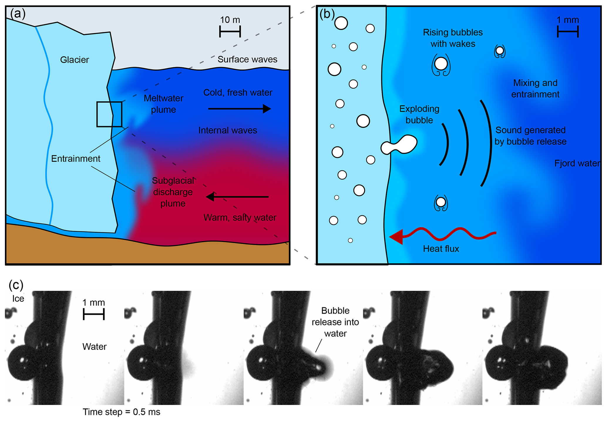
Figure 1 (a) A schematic of ice–ocean interactions at tidewater glaciers, including many processes that occur on scales of 10–100 m. These include subglacial discharge, water circulation in the fjord, and thermohaline structure. (b) An inset showing processes that occur within the proximal ice–water boundary, at scales ranging from roughly 0.1–100 mm. These include the release of air bubbles into the water, the rise of air bubbles through the water, and mixing within the proximal boundary. These smaller-scale processes have the potential to control heat flux across the boundary and into the ice. (c) Still frames from high-speed video footage of a bubble being released from glacier ice in a laboratory experiment.

The proximal boundary consists of a solid–liquid interface, and the class of problems describing the diffusion of heat in a medium accompanied by a change of phase state is referred to as Stefan problems (Rubinštein, 1971). This particular Stefan problem is complicated by the presence of salt in the water, gas which moves from the ice into the water, and processes that play out across a wide range of scales, as shown in Fig. 1. Theoretical frameworks to describe the proximal boundary are an active area of research. Current theoretical descriptions are based on conservation of heat and salt at the ice–water interface (Hellmer and Olbers, 1989; Holland and Jenkins, 1999). This description is combined with buoyant plume theory to describe the effects of rising meltwater and, in the case of glacier termini, subglacial discharge water on the fluxes across the proximal boundary (Jenkins, 2011; Cowton et al., 2015; Slater et al., 2016). This framework is largely untested by direct observations (Straneo and Cenedese, 2015; Cenedese and Straneo, 2023), and does not include gas effects. A large number of laboratory experiments have been conducted to study processes occurring at the ice–water interface (McCutchan and Johnson, 2022). Many of these incorporate the effects of both heat and salt, but realistic effects of the pressurized bubbles present in glacier ice are difficult to reproduce in the laboratory. Wengrove et al. (2023) have suggested that processes related to the release of pressurized bubbles from the ice could impact the boundary layer and affect heat transport through the proximal boundary. Results from numerical modelling studies on the scale of the proximal boundary have shown general agreement with some laboratory studies in terms of the observed melt rates and the structure of the thermal and velocity boundary layers (Wells and Worster, 2011; Gayen et al., 2016), but neither the laboratory studies nor the numerical simulations include the effects of pressurized bubbles.

There are indications that the description of fluxes across the ice–water boundary currently in use needs to be improved in order to allow for accurate estimates of submarine melt rates. Recent observational studies comparing plume-theory-derived estimates of subglacial melting with direct observations of terminus ablation from acoustic surveys (Sutherland et al., 2019) and estimates of melting based on hydrographic data (Jackson et al., 2020) have suggested that the current theoretical framework underestimates submarine melting outside of subglacial discharge plumes. Laboratory studies have also indicated that the existing framework may perform poorly when water velocities are slower. Specifically, the existing framework implicitly assumes that the boundary layer thickness is governed by a shear instability, but at low flow speeds it may instead be controlled by a convective instability (McConnochie and Kerr, 2017).

Improving the description of fluxes across the ice–water boundary will require a combination of theoretical studies, laboratory experiments, and field observations. Several recent papers have suggested adjustments to the existing parameterizations in order to better match field observations (Jackson et al., 2022; Schulz et al., 2022). This is an excellent step and should be supported by theoretical and laboratory studies. Direct observations of the proximal boundary at glacier termini are likely to remain elusive, due to the difficult and dangerous nature of conducting measurements near calving fronts of glaciers (Herrero, 2018). Recently, robotic vehicles have been used to make observations of water properties close to the termini of tidewater glaciers (Slater et al., 2018; Poulsen et al., 2022) or beneath floating ice shelves (Washam et al., 2023), but making measurements in the proximal boundary layer of vertical ice faces remains a challenge. Observations of the proximal boundary at small growlers can provide a natural laboratory and a bridge to better understanding of the physical processes that may occur there. This paper describes an apparatus to make such observations, which we have termed “the ice frame”, and the associated methods for its use. It also briefly presents some example data that were collected using the ice frame.

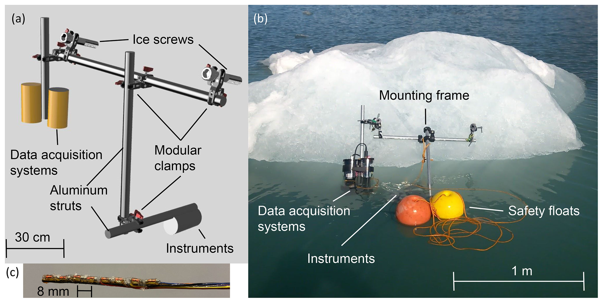
Figure 2 (a) Schematic of the ice frame. The main structure consisted of aluminium struts fastened together with a series of adjustable clamps. Two ice screws were screwed into a floating growler and the frame was attached to the screws using clamps. Instruments, which consisted of either a thermistor array or a camera and hydrophone, were fastened to the frame, allowing them to be held within the proximal boundary of floating growlers. (b) An image of the ice frame deployed on a floating growler in Hornsund Fjord, Svalbard. (c) The thermistor array used to measure temperature gradients in the water. Each orange cylinder is an individual glass-coated thermistor, separated with 8 mm spacing.

2 Methods

2.1 Description of the ice frame

The ice frame consisted of a collection of aluminium tubes which could be fastened together using adjustable clamps. Ice screws were used to fasten the frame to a growler, and instruments could be attached to the frame using clamps and held within the proximal boundary. Figure 2a shows a schematic of the most successful configuration of the frame, and Fig. 2b is a picture of the frame deployed on a floating growler. Details of the specific hardware elements of the ice frame are given in Appendix A. A camera, hydrophone, and microthermistor array were deployed on the frame. A detailed description of those sensors is given in Appendix B.

2.2 Design principles

There were four key principles that guided the design of the ice frame and the instruments deployed on it. First and foremost, the frame had to be simple to deploy. Attaching equipment to a piece of floating ice from a small boat is a difficult feat even in ideal conditions. Using only two ice screws, and placing them above the waterline, was key to keeping the frame deployment simple. Earlier iterations of the frame that included three or four points of contact with the ice, above and below the waterline, worked well during laboratory testing but proved to be too difficult to work with in the field. Second, the frame had to be adjustable in order to accommodate the natural variability in the surface of growlers. However, it also had to be easy to lock all of the moving parts into place once the frame was positioned correctly, in order to hold the instruments fixed relative to the ice face. Third, the frame, and instruments deployed on it, had to be sufficiently robust to hold up to inevitable bumping and banging during deployment and recovery. Finally, the components of the frame, and the instruments, had to be inexpensive and replaceable because there was a non-trivial chance that the frame and any instruments on it could be damaged or lost during the deployment.

2.3 Deployment

The field campaign described here was conducted in Hornsund Fjord, Svalbard. The Polish Polar Station, which is located on the north side of the fjord near the mouth, was used as a base of operations for the duration of the campaign. The frame was deployed from a zodiac crewed by two to three people, on growlers that were floating in the water. Some of the growlers were in the bay of Hansbreen glacier, which is about 2 km northeast of the station, and others were near the northern shore of the main arm of the fjord, between the station and Hansbreen.

There were several criteria involved in the selection of growlers on which to deploy the frame, the most important being location. The chosen growler had to be a safe distance (at least a few hundred metres) from the glacier terminus and from any large icebergs, so that calving events or iceberg rolling or disintegrating would not pose a danger to the boat crew. It also had to be sufficiently far from shore that the boat would not be at risk of running aground. Attention had to be paid to the surface currents and wind, to predict whether a growler that was in a safe spot at the time of selection might move to an unsafe location over the expected duration of the deployment. Aside from safety concerns, it was also important to choose a growler that was fairly isolated and not surrounded by thick melange or other growlers that would make navigating the boat difficult and could potentially damage the frame while it was deployed.

The other selection criteria were related to the size and shape of the growler itself. Deployment and recovery of the frame required the boat to be parked up against the growler for several minutes, with crew members leaning over the side of the boat holding it in position, fastening ice screws, and adjusting various elements of the frame. This involves an element of risk, which is exacerbated by the potential for floating ice to behave unpredictably, either rolling over or breaking apart. One way in which this risk was mitigated was by selecting growlers of appropriate size. The growler had to be large enough for the ice frame to fit onto it and present an approximately vertical face extending at least a half a metre below the waterline and about 30 cm above it but not so large as to pose a danger to the boat and crew in the event that it might suddenly break apart or roll over. The growlers that were selected were typically about 3–5 m in length and width, with a surface expression of about half a metre.

In addition to size, the geometry of the growlers played a role in the selection process. Growlers that were compact and looked sturdy were preferred over those that had protrusions or weak points that might have broken and caused sudden movement. Among growlers that seemed unlikely to break apart, it was also a priority to select those which seemed to be stable in the water and not likely to roll over. This was assessed by observing the response of the growler to the ambient wave field or to initial attempts to fasten ice screws to the growler.

Often it was useful to screw an extra ice screw into the growler initially to serve as hold to keep the boat in position while deploying the frame. The two ice screws to which the frame would be attached were then screwed into the ice. The instruments were attached to the frame and adjusted, based on visual estimation, to try to accommodate the geometry of the ice face to which the frame would be attached. The safety floats were fastened to the frame using a line. The frame was then lowered over the side of the boat, between the boat and the growler, and the crossbeam was attached to each of the two ice screws using pairs of SmallRig clamps. See Fig. 2 for a schematic and image of the frame.

Once the frame was successfully deployed, the boat would be moved some distance away (about 50–100 m) in order to minimize any unnecessary impacts on the environment that might influence the measurements but would be kept close enough to monitor the growler and frame. The frame would be recovered in a similar manner to that in which it was deployed.

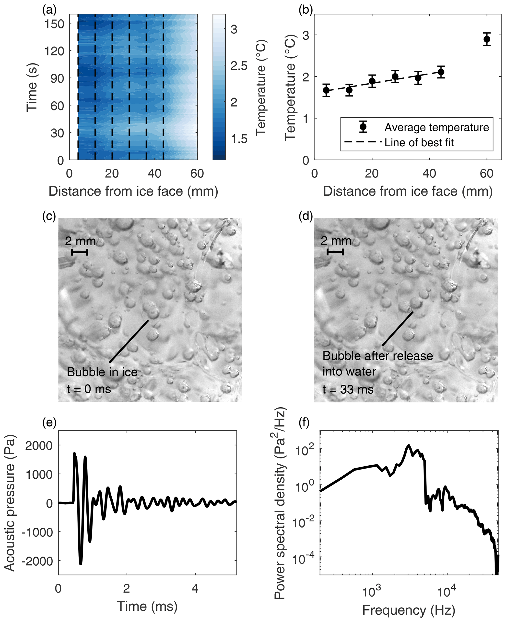
Figure 3 Example data collected using the ice frame. (a) Contour plot of the temperature observed in the proximal boundary of a floating growler, about 30 cm below the surface of the water. The x axis is distance from the ice face, and the position of individual thermistor elements is shown by the vertical dotted lines (Johnson et al., 2022). (b) Average (circles) and standard deviation (bars) of the temperature measured at each thermistor for the data displayed in panel (a). The linear least-squares fit to the first six elements (dashed line) has a slope of 0.01 mm ^∘C⁻¹. (c) Still frame from the underwater camera in which bubbles trapped in the ice are visible. (d) Another still frame from 33 ms later, just after the annotated bubble has been released from the ice. (e) Recording made by the hydrophone of the acoustic pulse released by the bubble shown in panels (c) and (d). (f) Power spectrum of the acoustic signal shown in panel (e), which has a broad peak centred around 4 kHz.

3 Results

3.1 Performance

As a mounting system, the ice frame has length, time, payload, and placement performance specifications. The frame is deployable on growlers ranging in size from 3–5 m across and provides access to the top 0.5–1 m of the ice–water interface. Instruments can be placed from the ice face up to about 0.5 m away. Under the conditions experienced during this field campaign, with air temperatures in the range of about 5–8 ^∘C and water temperatures in the range of about 2–4 ^∘C, and with ice screws of length 19 cm, the deployment time was limited to about 1–2 h before melting around the ice screws would make the frame-to-growler connection unstable. This might be extended with longer screws or in colder temperatures. Practical experience with the frame and a boat suggests that payloads up to about 5 kg can be managed. Three different types of data were successfully collected using the frame: images of the ice face, acoustic recordings, and temperature array measurements. These are described in greater detail below. In principle, other types of data could also be collected using a similar apparatus, such as the salinity of the water, flow speed in the water, or ablation of the ice face itself. The modular nature of the frame means that multiple instruments can be deployed at once, with the trade-off being increased weight and complexity.

3.2 Imaging of the ice face

The ice frame is well-suited to collecting direct-view images of the ice at close range. Using a camera mounted on the frame and positioned about 12 cm from the ice face, images of the ice face were successfully collected during this deployment. The camera resolution of about 25 µm per pixel at the ice face (see Appendix B1 for camera specifications) was sufficient to resolve individual bubbles in the ice and in the water. It should be noted that, since the index of refraction for ice is much closer to that of water than to that of air, it is easy to view bubbles within the ice but difficult to discern the ice–water boundary itself in direct-view images. A wider field of view could be obtained by mounting the camera further from the ice, but this would create some difficulties: first, water clarity potentially becomes an issue, and second, the logistics of attaching a sensor to the frame increases in difficulty the further from the ice the sensor is.

Two still frames from the camera video data are presented in Fig. 3c and d. In panel c, the bubble annotated near the centre of the frame is still fixed within the ice. In panel d, several frames later, it has been released into the water and has started to rise and move slightly to the right. The camera depth of field was very shallow, enabling an estimate of the size of objects which are in focus. The radius of this bubble was estimated to be 0.8 mm.

3.3 Acoustic recordings

The ice frame allowed the collection of acoustic data at close proximity to the ice face of a melting growler. (See Appendix B1 for instrumentation details.) Placing a hydrophone in such close proximity to the ice face allows for the clear identification of the pulses of sound released by individual bubbles of air as they are released from the melting ice. One difficulty that should be noted is that placing a hydrophone in such close proximity to the ice face results in absolute sound pressure levels that are too high for many off-the-shelf hydrophones to measure, resulting in clipped signals. Care needs to be taken to ensure that the sensitivity of the hydrophone and recording system is not too high. The hydrophone used in this study had a sensitivity of −208 dB referenced to 1 V µPa⁻¹, and it was used with no pre-amplifier.

The video and acoustic data were collected at the same time, and the data streams were synchronized, allowing for the identification of bubbles visible in the video data in the acoustic record. The acoustic pulse emitted by the bubble seen in Fig. 3c and d is shown in Fig. 3e. The power spectrum of this pulse is presented in Fig. 3f and displays a broad peak centred around 4 kHz. This is roughly consistent with the expected natural frequency of 3.9 kHz of a bubble of radius 0.8 mm, based on the formula derived by Minnaert (1933).

3.4 Temperature measurements

The ice frame allowed for the successful collection of in situ measurements of water properties in the proximal boundary. Using an array of calibrated thermistors (see Appendix B2 for details), the profile of the water temperature orthogonal to the ice face of a floating growler about 30 cm below the surface was measured over a span of about 20 min. A contour plot of a subset of this temperature data is shown in Fig. 3a. There is some temporal variability that may be related to wave action or changes in water flow past the ice face, but in the absence of any additional measurements, it is difficult to determine the cause or nature of these variations. It is also possible that these fluctuations could be caused by small motions of the frame and the sensors relative to the growler. Nevertheless, the overall thermal structure observed is quite consistent, as shown by Fig. 3b. The gradient across the six sensors nearest to the ice face is 0.01 ^∘C mm⁻1, with a steepening outside of this region. The temperature at the sensor 4 mm from the ice face is in excess of 1.5 ^∘C, implying that the temperature gradient must be substantially greater within the first few millimetres of the ice face, since the temperature of the interface itself should be almost 0 ^∘C.

4 Discussion and conclusions

The ice frame allows for direct in situ measurements at the ice surface, and in the water up to about 0.5 m from the ice, at floating growlers. There are obvious differences between the ice–ocean boundary at floating growlers and at a glacier terminus, such as the vertical scale of the ice wall and the potential presence of subglacial discharge plumes. However, some of the physical processes and dynamics on sub-metre scales may be common between the two environments. These may include the release of air bubbles into the ice or other processes that modulate heat flux within the proximal boundary. Floating growlers may therefore be an effective natural laboratory that can be used to study ice–ocean interactions at these scales, with relevance to glacial termini. This boundary is more realistic than one that can be recreated in the lab with artificial ice and also more easily accessible than the terminus itself.

The study of floating ice in glacial bays is also consequential in its own right. This ice can play an important role in controlling conditions in glacial fjords (Davison et al., 2020). Understanding small-scale processes that modulate the interaction of floating ice with water in the fjord can aid understanding of the fjord-scale influence of floating ice.

Extension of the ice frame, or similar apparatuses, to allow for deployment at the terminus itself, and at greater depths below the surface, is a natural future direction of research. The risk of calving icebergs means that any such deployment will need to be carried out with uncrewed robotic vehicles. Uncrewed vehicles have been used recently to conduct surveys near glacial termini (Slater et al., 2018) but not to make measurements within the proximal boundary itself. Making these types of measurements is challenging but may be necessary for the effort to accurately describe fluxes and melting at the termini of tidewater glaciers.

Appendix A: Frame design

The ice frame consisted of several components, each of which is identified in Fig. 2a. The main structure was made up of hollow cylindrical aluminium tubes. The tubes were 75 cm long with a 1 in. outer diameter and 0.065 in. wall thickness. The tubes were held together with two different types of clamps. Off-road light bar mounting brackets, manufactured by Mosleyz, were used for joints that did not need to be adjusted in the field. Pairs of SmallRig Super Clamps, fastened to either end of a $\mathrm{3}/\mathrm{8}$ in. stainless steel threaded rod, were used for connections that needed to be made or adjusted during the deployment process. Two Petzl 19 cm ice screws were used to fasten the frame to the ice. Finally, a pair of flotation spheres was used to prevent the frame from sinking. Marine grease was used to lubricate and protect any corrosion-sensitive elements, such as nuts, bolts, and threaded rods. When disassembled, the entire frame fit into a single Zarges box of dimensions $\mathrm{0.8}\times \mathrm{0.4}\times \mathrm{0.4}$ m. The total weight of the frame and instruments together was about 5 kg, which was sufficiently light as to be manageable for deployment by hand over the side of a small boat. The total cost of the frame hardware was about USD 300, with the single most expensive component being the ice screws.

To deploy the frame, the ice screws were first screwed into the growler face about 20 cm above the waterline, with a horizontal separation of about 60 cm. A horizontal crossbeam was then attached to both screws with pairs of adjustable SmallRig clamps. A vertical beam with a length of 75 cm was fastened to this crossbeam at a right angle using the Mosleyz bar mounting brackets and extended down below the surface of the water. The instruments were attached to the bottom of this vertical beam using pairs of adjustable SmallRig clamps. Since the top of the vertical beam was fastened to the cross beam within 5–10 cm of the ice, as long as the ice face was roughly vertical, the force of gravity would act to pull the instruments down and in towards the ice. In some cases, the instruments themselves formed the third point of contact with the ice face. In other cases, an additional aluminium tube was connected to the bottom of the vertical beam and formed the third point of contact with the ice face, and the instruments were either attached to this tube or to the vertical beam. The flotation spheres were tied to one end of a 5–10 m long rope, with the other end tied to the main structure of the frame.

Appendix B: Instruments

B1 Hydrophone and camera

An underwater camera and a hydrophone were used to make coincident optical and acoustic observations of air bubbles being released from the ice. The camera was a GoPro Hero 5, modified using a Back-Bone lens adapter and a Schneider 17 mm lens. A resolution of 1080p and frame rate of 120 frames per second were used. A Voltaic V25 USB battery pack was used to extend the battery life of the GoPro. The camera and the battery pack were contained in a 4 in. diameter watertight enclosure from Blue Robotics. The total cost of the camera assembly and enclosure was about USD 1000. The enclosure was attached to the bottom of the vertical beam of the frame using a SmallRig clamp on one end of a threaded rod, with the other end screwed into a plate which was mounted to the back end of the enclosure using Blue Robotics enclosure clamps. A pair of wooden rods was fastened to the sides of the enclosure, extending out past the front face to the focal plane of the camera, which was about 12 cm beyond the front face of the enclosure. When the frame was deployed on a growler, the rods would rest against the submerged ice face and hold the camera an appropriate distance from the ice face such as to place it within the focal plane of the camera. A GoPro Smart Remote was used to turn the camera on and start recording before putting the frame in the water, allowing the watertight enclosure to remain sealed.

An AS-1 hydrophone, from Aquarian Scientific, was used to make acoustic recordings at close proximity to the ice face. The sensitivity of the AS-1 hydrophone was −208 dB re 1 V µPa⁻¹. The hydrophone was mounted on one of the wooden standoff rods, about 7 cm from the ice face. The hydrophone cable was cut to a length of about 2 m and spliced to an Impulse underwater connector. The recording system for the hydrophone consisted of a Tascam DR40-X handheld recorder, with a unity-gain, high-impedance buffer between the hydrophone output and the Tascam input. The recording system was housed in a 3 in. diameter Blue Robotics watertight enclosure. An external switch was connected to an Adafruit Feather microcontroller, which emulated a Tascam RC-10 remote control (see GitHub repository at https://github.com/abbrev/tascam-rc-10-remote, last access: 23 April 2022), allowing the Tascam to be turned on and start recording without opening the enclosure. The total cost of the hydrophone, recording system, and enclosure was about USD 1000. The video and audio data from the camera and hydrophone were synchronized by starting recording of both instruments and then placing the hydrophone in the field of view of the camera and tapping it.

B2 Thermistors

Another instrument configuration that was successfully deployed during this campaign was a thermistor array. The array consisted of eight individual MF58 3950B 10 kΩ glass-encapsulated thermistors. The thermistors were glued to a 2 mm diameter carbon fibre rod. A silicone spacer about 2 mm thick was placed between the rod and each thermistor in order to help isolate the elements from the thermal mass and conductivity of the rod. Wires of gauge 30 AWG were soldered to the ends of the thermistors. A common ground wire, and eight signal wires, ran from the array to a Blue Robotics watertight enclosure containing the acquisition electronics. The exposed solder joints of the array were coated with polyurethane and then silicone in order to make the array waterproof. The data were recorded by an Adafruit Feather microcontroller, using two ADS1115 16-bit four-channel analogue-to-digital converters. For each channel, the output of a voltage regulator was connected by a 27.2 kΩ resistor to the appropriate analogue-to-digital input, which was then connected to one of the resistor signal wires. The total cost of the thermistor array and housing was about USD 500.

During deployment, the thermistor array was fastened to the bottom of the vertical beam of the frame using a pair of SmallRig clamps. The array was positioned to extend out from the frame towards the growler, perpendicular to the ice face. An aluminium rod was also connected to the bottom of the vertical beam, extending out towards the ice face but at an angle of about 20^∘ below horizontal. The rod and array were adjusted such that the rod would support the weight of the frame against the ice, while the array would just barely touch the ice face.

The Steinhart–Hart equation was used to compute the estimated temperature of each thermistor given the measured resistance. The optimal parameters for each individual element were determined by calibrating the array against an RBR Solo temperature logger. The array and the RBR Solo were both placed in a well-mixed bucket of seawater. This was done repeatedly, with water temperatures ranging from about −1 to 10 ^∘C in increments of about 0.5 ^∘C. The computed temperature of each array element using the Steinhart–Hart equation was then fit to the “true” temperature measured by the RBR Solo using linear regression.