Sources of low-frequency variability in observed Antarctic sea ice

Antarctic sea ice has exhibited significant variability over the satellite record, including a period of prolonged and gradual expansion, as well as a period of sudden decline. A number of mechanisms have been proposed to explain this variability, but how each mechanism manifests spatially and temporally remains poorly understood. Here, we use a statistical method called low-frequency component analysis to analyze the spatiotemporal structure of observed Antarctic sea ice concentration variability. The identified patterns reveal distinct modes of low-frequency sea ice variability. The leading mode, which accounts for the large-scale, gradual expansion of sea ice, is associated with the Interdecadal Pacific Oscillation and resembles the observed sea surface temperature trend pattern that climate models have trouble reproducing. The second mode is associated with the central Pacific El Niño–Southern Oscillation (ENSO) and the Southern Annular Mode and accounts for most of the sea ice variability in the Ross Sea. The third mode is associated with the eastern Pacific ENSO and Amundsen Sea Low and accounts for most of the pan-Antarctic sea ice variability and almost all of the sea ice variability in the Weddell Sea. The third mode is also related to periods of abrupt Antarctic sea ice decline that are associated with a weakening of the circumpolar westerlies, which favors surface warming through a shoaling of the ocean mixed layer and decreased northward Ekman heat transport. Broadly, these results suggest that climate model biases in long-term Antarctic sea ice and large-scale sea surface temperature trends are related to each other and that eastern Pacific ENSO variability is a key ingredient for abrupt Antarctic sea ice changes.

1 Introduction

Antarctic sea ice plays a crucial role in Earth's climate system. The seasonal cycle of Antarctic sea ice cover, which expands and contracts by approximately 16 million km² each year, impacts the ocean's global overturning circulation through brine rejection and freshwater input (e.g., Abernathey et al., 2016; Pellichero et al., 2018). Antarctic sea ice cover also exerts a strong control on Southern Ocean primary productivity (e.g., Arrigo et al., 1997; Lizotte, 2001; Arrigo and van Dijken, 2004; Smith and Comiso, 2008), carbon exchange (e.g., Fogwill et al., 2020), and low-level clouds (e.g., DuVivier et al., 2021) by modulating air–sea heat, freshwater, and biogeochemical fluxes. Studies have also invoked Antarctic sea ice as a major player in glacial–interglacial cycles of the late Pleistocene through reorganization of the ocean's global overturning circulation (e.g., Keeling and Stephens, 2001; Ferrari et al., 2014; Marzocchi and Jansen, 2017). Understanding processes that contribute to trends and variability in observed Antarctic sea ice remains a central goal of climate science.

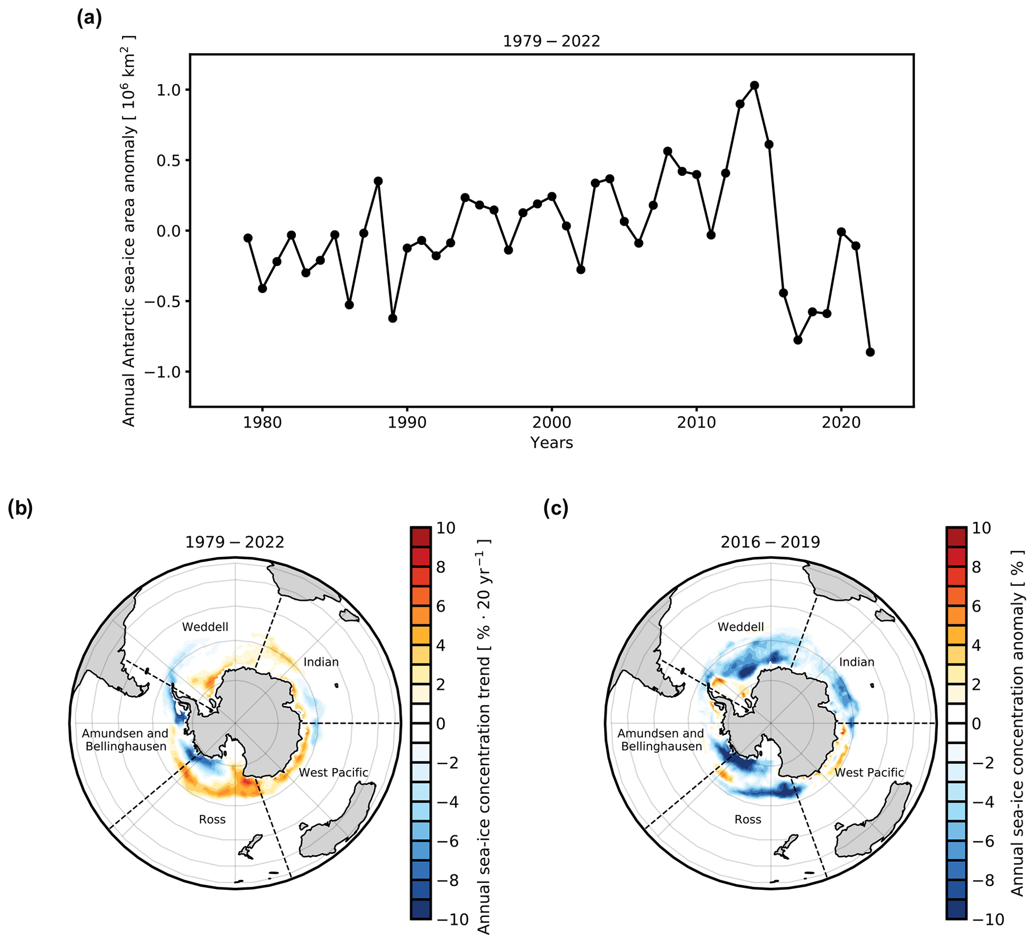
Figure 1 Observed changes in Antarctic sea ice from 1979 to 2022. (a) Anomalies in annual-mean Antarctic sea ice area from 1979 to 2022 relative to the 1981–2010 average. (b) Linear trend in annual-mean Antarctic sea ice concentration from 1979 to 2022. (c) Anomalies in annual-mean Antarctic sea ice concentration averaged from 2016 to 2019 relative to the 1981–2010 average. Annual-mean Antarctic sea ice area exhibits a slight positive trend of 0.15 × 10⁶ km²⋅40 years⁻¹ from 1979 to 2022, and the SIA anomaly averaged from 2016 to 2019 is approximately −0.60 × 10⁶ km². The regions have longitude boundaries of 60° W–20° E (Weddell), 20–90° E (Indian), 90–160° E (West Pacific), 160° E–130° W (Ross), and 130–60° W (Amundsen and Bellingshausen).

Antarctic sea ice has experienced notable changes over the satellite record. Since the late 1970s, Antarctic sea ice area (SIA) has slowly increased, despite significant global warming (Fig. 1a; Parkinson and Cavalieri, 2012; Turner et al., 2015; Gagné et al., 2015; Parkinson, 2019). The increase in Antarctic SIA occurred largely between 2000 and 2014 (Fig. 1a; Gagné et al., 2015; Meehl et al., 2016; Simmonds and Li, 2021) and was driven by an increase in sea ice concentration in all sectors of the Antarctic, except for the Amundsen and Bellingshausen seas (Fig. 1b). However, in 2016, Antarctic SIA experienced an abrupt decline that persisted until 2019 and occurred again in 2022 (Fig. 1a; Turner et al., 2017; Stuecker et al., 2017; Raphael and Handcock, 2022; Fogt et al., 2022). The abrupt decrease in Antarctic sea ice concentration between 2016 and 2019 occurred mainly in the Weddell Sea, Indian sector, and Ross Sea (Fig. 1c; Turner et al., 2017).

A number of mechanisms have been proposed for both the gradual expansion of and abrupt decline in Antarctic sea ice. Meehl et al. (2016) argued that the gradual increase in Antarctic sea ice was caused by decadal climate variability emanating from the tropical Pacific that deepened the Amundsen Sea Low, strengthened the circumpolar westerlies, and caused surface cooling through enhanced northward Ekman heat transport. Other studies argued that increased freshwater input, either from ice shelf melt (Bintanja et al., 2013; Pauling et al., 2016; Sadai et al., 2020), changes in precipitation and evaporation (Fyfe et al., 2012; Purich et al., 2018), or sea ice melt itself (Haumann et al., 2020), can cause sea ice expansion by increasing subsurface stratification and preventing warmer, deeper waters from interacting with the surface. Antarctic sea ice expansion has also been attributed to internal climate variability and variations in open-ocean convection (Turner et al., 2016; Singh et al., 2019; Zhang et al., 2019). The abrupt decline in Antarctic sea ice, on the other hand, has been attributed to weakened circumpolar westerlies associated with intrinsic variability of the Southern Annular Mode (SAM), El Niño–Southern Oscillation (ENSO), and Indian Ocean Dipole (IOD; Stuecker et al., 2017; Schlosser et al., 2018; Wang et al., 2019; Purich and England, 2019). The abrupt decline in sea ice has also been attributed to a gradual build-up of subsurface heat through ocean preconditioning (Meehl et al., 2019; Campbell et al., 2019; Zhang et al., 2022).

Beyond the gradual expansion and abrupt decline in Antarctic sea ice, Antarctic sea ice also exhibits substantial interannual-to-decadal variability, which has been linked to the phasing of the SAM and ENSO (Thompson and Solomon, 2002; Fogt and Bromwich, 2006; Stammerjohn et al., 2008; Simpkins et al., 2012; Matear et al., 2015; Doddridge and Marshall, 2017; Holland et al., 2017; Crosta et al., 2021), zonal atmospheric wave structures (Raphael, 2007), surface wind variability (Holland and Kwok, 2012), Pacific decadal variability (Chung et al., 2022), and Atlantic multidecadal variability (Li et al., 2014; Eayrs et al., 2021). Indeed, a number of mechanisms can contribute to short- and long-term Antarctic sea ice variability, but a unified understanding of how each process manifests spatially and temporally in the observational record is lacking.

This lack of understanding is, in part, because most coupled climate models – which oftentimes aid in a mechanistic understanding of the climate system – have trouble reproducing the observed magnitude, sign, and spatial pattern of Antarctic sea ice trends, including periods of abrupt sea ice loss (Turner et al., 2013; Purich et al., 2016; Rosenblum and Eisenman, 2017; Roach et al., 2020). Some studies have shown that internal climate variability may explain the disagreement in Antarctic sea ice trends between climate models and observations (Polvani and Smith, 2013; Zunz et al., 2013; Mahlstein et al., 2013; Gagné et al., 2015; Singh et al., 2019). Other studies have shown that climate models can reproduce the sign and magnitude of observed Antarctic sea ice trends if winds or sea ice motion are nudged to observed values (e.g., Blanchard-Wrigglesworth et al., 2021; Sun and Eisenman, 2021), which suggests an important role for the strengthening of near-surface winds in Antarctic sea ice expansion and possibly ozone depletion, which has caused increased winds (Thompson and Solomon, 2002). However, ozone depletion has been shown to cause little sea ice expansion in climate models (Sigmond and Fyfe, 2010, 2014; Polvani et al., 2021), which complicates the mechanistic understanding of the observed sea ice changes. Reconciling climate models and observations requires a better understanding of the sources of sea ice trends and variability in the observational record.

In this study, we use low-frequency component analysis (LFCA; Wills et al., 2018; Schneider and Held, 2001), which identifies slowly evolving modes of variability, to examine low-frequency variability in observed Antarctic sea ice concentration. While LFCA is a statistical method, it makes no a priori assumptions about the processes or regions that contribute to low-frequency sea ice variability. Additionally, while LFCA isolates low-frequency variability, it still retains high-frequency variability, enabling a robust characterization of sea ice variability across timescales. In what follows, we first describe LFCA and the observational datasets (Sect. 2). We then use LFCA to explore how different modes of variability have contributed to observed Antarctic sea ice changes (Sect. 3). Finally, we examine mechanisms for low-frequency Antarctic sea ice variability (Sect. 4).

2 Data and methods

2.1 Observations

Estimates of monthly Antarctic sea ice concentration were obtained from version 4 of the NOAA/NSIDC Climate Data Record of passive microwave sea ice concentration (Meier et al., 2021a). Similar results are found when using sea ice concentration obtained from the Ocean and Sea Ice Satellite Application Facility (OSI SAF; Lavergne et al., 2019). Reanalysis data of sea surface temperatures (SSTs), 500 hPa geopotential height (GPH), 10 m (near-surface) zonal and meridional winds (u_s and v_s), and the net surface heat flux were obtained from the ERA5 global reanalysis (Hersbach et al., 2020). Sparse data coverage of the Southern Ocean toward the beginning of the satellite era motivates the use of reanalysis data. We further use an estimate of the surface ocean mixed-layer depth from the companion ORAS5 global ocean reanalysis (Zuo et al., 2019). While the choice of ocean reanalysis introduces errors into physical interpretations, we prefer reanalysis over direct observations for the spatial and temporal coverage. All sea ice and reanalysis data products contain monthly data from 1979 to 2022 and are used to compute annual means. We discuss the effect of seasonality in Sect. 5 but limit ourselves to the annual timescales for this study. The sea ice and reanalysis data products are regridded to a 1° × 1° grid using second-order conservative remapping.

2.2 Low-frequency component analysis

LFCA is a statistical method that finds the linear combination of empirical orthogonal functions (EOFs) that results in the highest ratio of low-frequency variance to total variance (Wills et al., 2018; Schneider and Held, 2001). We define low-frequency variance as the variance remaining after applying a 10-year cutoff low-pass filter, similarly to previous studies that have applied LFCA to other climate variables (e.g., Wills et al., 2018; Årthun et al., 2021; Oldenburg et al., 2021; Dörr et al., 2023). LFCA has been used to characterize and understand modes of low-frequency variability in Atlantic and Pacific sea surface temperature (Wills et al., 2019a, b; Årthun et al., 2021), the Atlantic overturning circulation (Jiang et al., 2021), meridional ocean heat transport (Oldenburg et al., 2021), Southern Ocean surface winds (Dong et al., 2023), and Arctic sea ice concentration (Dörr et al., 2023), the latter of which is a companion study of this one.

In LFCA, the resulting anomaly patterns and time series are called low-frequency patterns (LFPs) and low-frequency components (LFCs), respectively (see Wills et al., 2018, for more details). In this study, the patterns and time series represent Antarctic sea ice concentration anomalies relative to a 1981–2010 average. The LFCs are normalized to have unit variance such that the LFPs show the anomaly pattern associated with a 1-standard-deviation anomaly in the corresponding LFC. The LFCs are required to be orthogonal (uncorrelated), but the LFPs are not. LFCA finds the pattern of variability within the included EOFs that has the maximum possible ratio of low-frequency variance to total variance and persistence, motivating its use over other statistical methods like dynamical adjustment (e.g., Smoliak et al., 2015) and principal component analysis (PCA). PCA, for example, takes advantage of the spatial structure of covariation in climate data to find a basis of EOFs that are ordered by the fraction of total variance they capture. Because of this, PCA maximizes the variance captured by the first EOF, and it can sometimes group together multiple processes and give spurious connections that are not rooted in shared physical mechanisms (e.g., Deser, 2000). LFCA instead identifies modes of variability based on their dominant timescale, providing a more physically consistent representation of variability in climate data.

The resulting LFPs are sorted by their ratio of low-frequency variance to total variance, which we refer to as the variance ratio (r). Here we retain the five leading EOFs, which account for approximately 70 % of the total Antarctic sea ice concentration variability. The choice of the number of EOFs to retain is subjective. We find that increasing the number of EOFs causes over-fitting issues that affect the physical interpretability, while decreasing the number EOFs to three accounts for less of the total sea ice concentration variability and mixes modes of ENSO variability that appear to be physically distinct.

To better quantify the role of each LFC in observed Antarctic sea ice, the LFCs and LFPs are used to construct temporally evolving maps of sea ice concentration anomalies. This is done by multiplying each LFP by the corresponding LFC. The reconstructed maps are further used to calculate regional and pan-Antarctic SIA anomalies by multiplying by the grid cell area and summing up over the target region. This produces a time series of Antarctic SIA anomalies unique to each LFC.

An improved understanding of the mechanisms related to sea ice variability can be achieved by performing a combined analysis of sea ice concentration with other fields like sea surface temperature or sea level pressure. This was introduced by Wills et al. (2020) using a signal-to-noise pattern recognition method (see also Bretherton et al., 1992). We performed a three-field analysis using SST and 500 hPa GPH and have determined that sea ice concentration alone is sufficient to isolate modes of low-frequency Antarctic sea ice variability. For the multi-field analysis, SST and GPH anomaly matrices are concatenated with the sea ice concentration anomaly matrix in the spatial dimension. Each field variable is normalized by the trace of its covariance matrix such that all variables are unitless and weighted equally. The rest of the multi-field analysis proceeds exactly as in the individual LFCA on sea ice concentration. Note, a companion study (i.e., Dörr et al., 2023) found that the combined analysis improved estimates of the forced (or anthropogenic) component of Arctic sea ice trends. We hypothesize that the multi-field approach works better for the Arctic because Arctic sea ice exhibits a stronger forced response associated with global warming than Antarctic sea ice does (e.g., Rosenblum and Eisenman, 2017).

3 Patterns of low-frequency Antarctic sea ice variability

We begin by examining the LFCs and LFPs obtained by applying LFCA to the annual-mean Antarctic sea ice concentration from 1979 to 2022 with a 10-year cutoff low-pass filter and retaining the five leading EOFs (see Sect. 2.2). Each LFP and LFC is spatially and temporally distinct, containing large regional structures in terms of Antarctic sea ice concentration and different characteristic timescales (Fig. 2). LFP1 exhibits a nearly pan-Antarctic-wide signal of positive sea ice concentration anomalies, with negative sea ice concentration anomalies in the Amundsen and Bellingshausen seas, and it accounts for approximately 30 % of the low-frequency variance (Fig. 2a). LFP1 is similar to the observed trend in Antarctic sea ice concentration (compare Figs. 1a and 2a) and has a relatively high variance ratio (r=0.70). The associated LFC exhibits a strong positive trend and a canonical red-noise spectra with increasing power at low-frequency (>10 years) timescales. LFC1 also captures the increased positive trend in sea ice concentration between 2000–2014 (Fig. 2a). LFP2 features a spatial pattern reminiscent of the SAM imprint on sea ice concentration (Lefebvre et al., 2004), with positive sea ice concentration anomalies in the Ross Sea and negative sea ice concentration anomalies in the Weddell Sea (Fig. 2b). LFP2 accounts for approximately 21 % of the low-frequency variance and has a smaller variance ratio (r=0.52) than LFP1. The associated LFC exhibits strong positive values in the late 1990s and strong power at approximately 3- and 7-year timescales. LFP3 shows a large-scale pattern of positive sea ice concentration anomalies mainly in and around the Weddell Sea (Fig. 2c). LFP3 accounts for approximately 12 % of the low-frequency variance and has a variance ratio of r=0.38. Notably, LFC3 captures the abrupt decline in sea ice concentration that occurred around 2016. Note that other LFCs also exhibit declines around 2016. However, LFC3 also captures abrupt decline events in 1988 and 2010 and the persistent negative sea ice concentration anomalies seen since 2016. LFC3 exhibits strong power around 4- and 5-year timescales, suggesting an association with ENSO (e.g., Trenberth, 1997). LFP4 has strong negative sea ice concentration anomalies in the Amundsen and Bellingshausen seas, with positive sea ice concentration anomalies in the Weddell Sea and Indian sector (Fig. 2d). LFP4 accounts for approximately 5 % of the low-frequency variance and has a small variance ratio (r=0.17). The associated LFC (LFC4) exhibits power on 3- and 4-year timescales. Figure A1 in the Appendix shows the last LFC and LFP, which essentially represent the residual from all higher-frequency sea ice variability (see power spectra). LFP5 weakly resembles the spatial pattern of sea ice concentration anomalies associated with atmospheric zonal wave three, as identified by Raphael (2007). LFC5 also shares some common features with the zonal wave three index (compare LFC5 with Fig. 7 of Raphael, 2007).

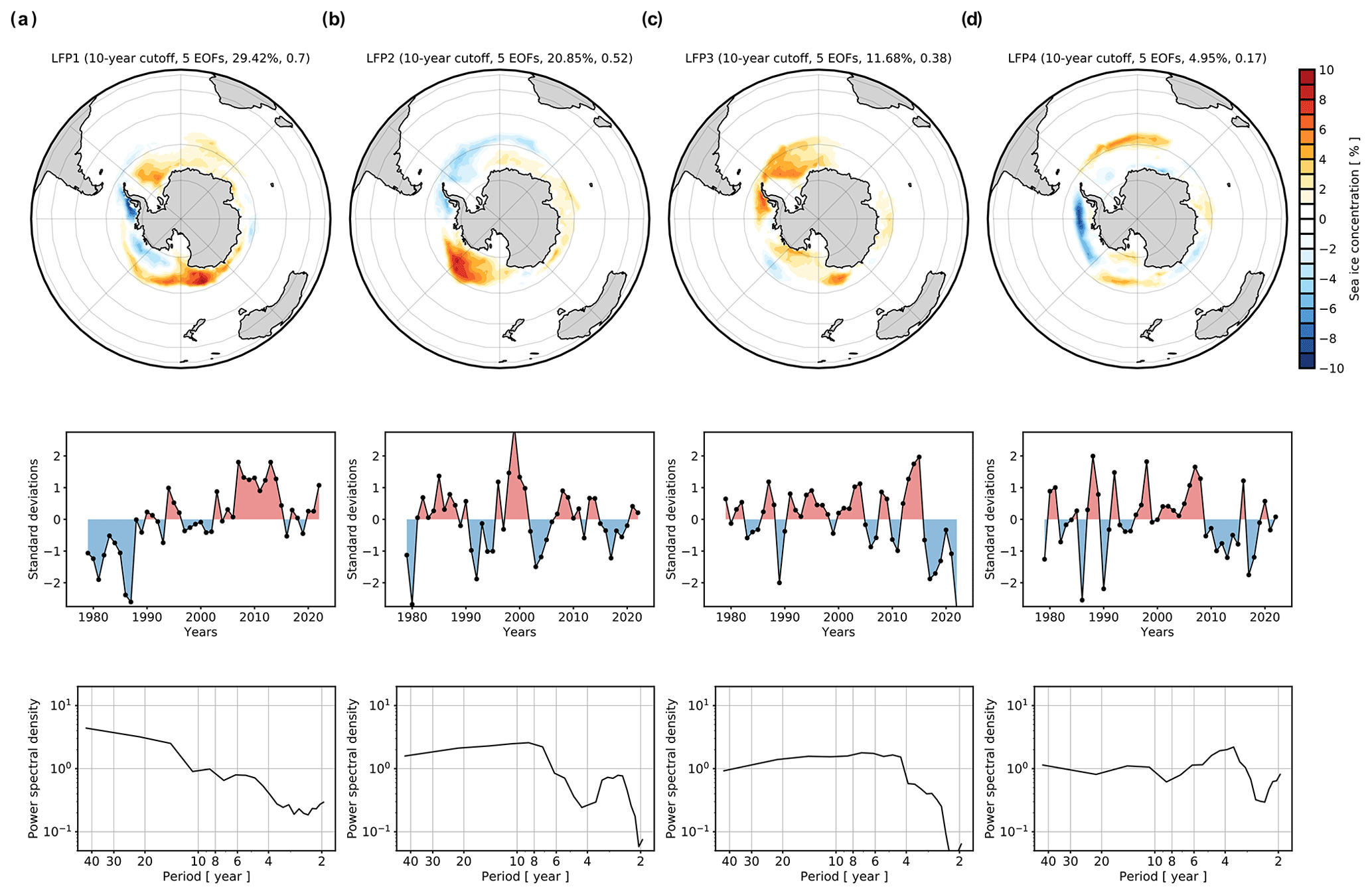
Figure 2 Low-frequency variations in Antarctic sea ice concentration. (a) First, (b) second, (c) third, and (d) fourth (top) low-frequency patterns (LFPs), (middle) low-frequency components (LFCs), and (bottom) power spectra density of each LFC using a 10-year cutoff and retaining the five leading EOFs of annual-mean Antarctic sea ice concentration anomalies from 1979 to 2022. Power spectra are computed with multitaper spectral analysis (Percival and Walden, 1993). The fraction of explained low-frequency variance (in %) and the ratio r of low-frequency variance to total variance is given for each pattern in the titles of the top panels.

3.1 Contribution to sea ice concentration trends and variability

We next consider how each LFC contributes to the trends and variability of observed Antarctic sea ice concentration from 1979 to 2022 by projecting each LFC onto the corresponding LFP at each grid point (see Sect. 2.2). This produces a time series of sea ice concentration at each grid point that is unique to each LFC.

The dominant mode contributing to the gradual increase in Antarctic sea ice concentration since the late 1970s is LFC1. A linear trend of the sea ice concentration associated with LFC1 shows large positive values throughout much of the Antarctic and weak negative values in the Amundsen and Bellingshausen Seas (Fig. 3a), which is consistent with the observed trend in sea ice concentration (Fig. 1a). The other three LFCs (Fig. 3b–d) contribute little to the long-term trend in Antarctic sea ice concentration. However, LFC3 does contribute to a slight negative trend in sea ice concentration in and around the Weddell Sea (Fig. 3c), though these values are smaller than the large positive values seen in LFC1 (Fig. 3a).

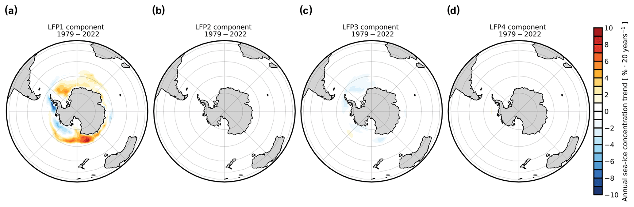
Figure 3 Trends in low-frequency components of Antarctic sea ice concentration. Linear trend in annual-mean Antarctic sea ice concentration anomalies from 1979–2022 associated with (a) LFC1, (b) LFC2, (c) LFC3, and (d) LFC4.

While LFC1 dominates the long-term trend in sea ice concentration, it contributes little to the abrupt decline in 2016 and in the years that followed (Fig. 4a). Antarctic sea ice concentration anomalies from 2016 to 2019 are primarily related to LFC2–4 (Fig. 4b–d). LFC2 contributed to a decline in sea ice concentration in the Ross Sea, while LFC3 contributed to a decline in sea ice concentration mostly in the Weddell Sea but also in other regions like the West Pacific sector and parts of the Ross Sea. LFC4 contributed some to the abrupt decline in sea ice concentration from 2016 to 2019, with small changes in the peripheral edge of the sea ice cover in the Weddell Sea and Indian sector (Fig. 4d).

3.2 Contribution to regional sea ice area changes

To better understand how each LFC contributes to the temporal evolution of Antarctic sea ice, we next examine the Antarctic SIA anomalies associated with each LFC and LFP (see Sect. 2.2). The regional domains broadly capture regions of distinct Antarctic sea ice variability, as noted by Raphael and Hobbs (2014). These regions include the Weddell Sea, Indian sector, West Pacific sector, Ross Sea, and Amundsen and Bellingshausen seas (see Fig. 1).

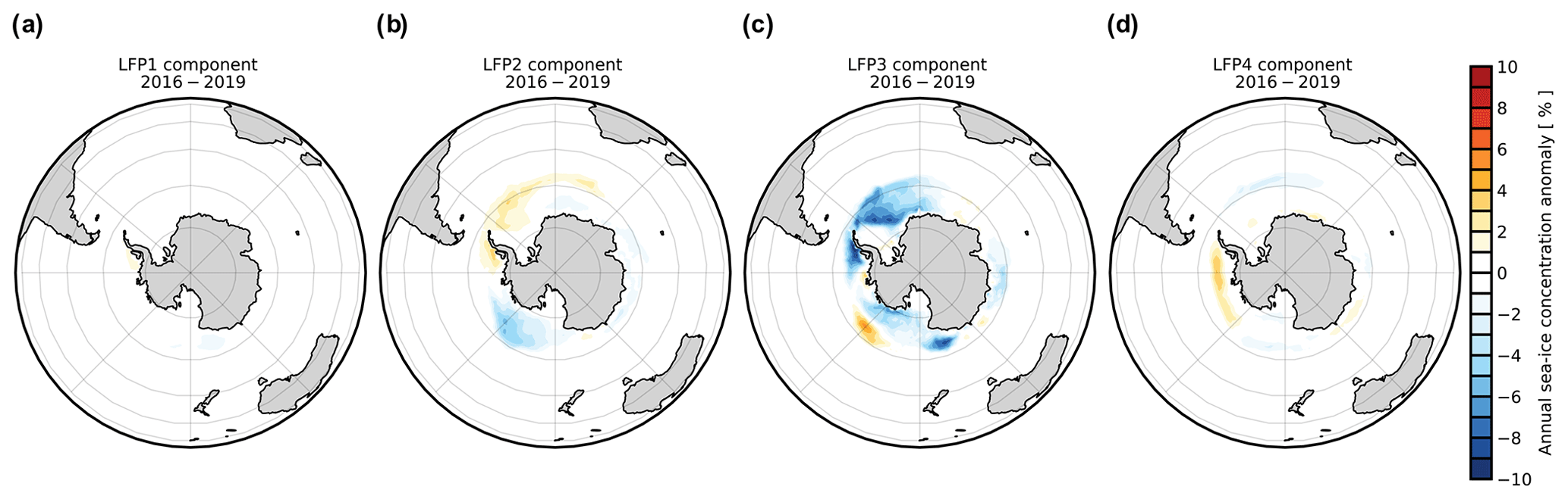
Figure 4 Anomalies in low-frequency components of Antarctic sea ice concentration. Anomalies in annual-mean Antarctic sea ice concentration during 2016–2019 associated with (a) LFC1, (b) LFC2, (c) LFC3, and (d) LFC4.

For pan-Antarctic SIA, LFC1 captures the long-term positive trend in Antarctic SIA (Fig. 5a) and accounts for approximately 20 % of the total SIA variability (Fig. 5b). The dominant contributor to pan-Antarctic SIA variability, however, is LFC3, which captures the abrupt decline in SIA around 2016 (Fig. 5a) and accounts for approximately 60 % of the total SIA variability (Fig. 5b). LFC3 also captures other periods of abrupt Antarctic SIA decline, such as the period around 1988, and closely follows the interannual variability in observed pan-Antarctic SIA. LFC2 contributes some to pan-Antarctic SIA variability (Fig. 5a), accounting for approximately 5 % of the total SIA variability (Fig. 5b). LFC4 contributes little to the pan-Antarctic SIA variability (Fig. 5a and b). Note both here and in the following paragraphs that the contributions from each LFC to SIA separately sum to be slightly greater than the contributions of all four LFCs combined due to the non-orthogonality of the associated LFPs.

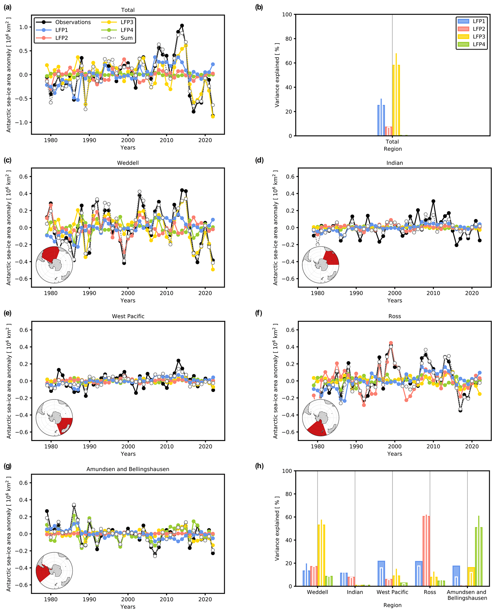
Figure 5 Low-frequency components of Antarctic sea ice area. (a) Annual-mean Antarctic sea ice area anomalies computed from the first (blue), second (red), third (yellow), and fourth (green) LFPs and LFCs. The sum of the three components is also shown (dashed gray line). (b) The proportion of variance explained in annual-mean Antarctic sea ice area anomalies for the LFP1 (blue), LFP2 (red), LFP3 (yellow), and LFP4 (green) components. Regional Antarctic sea ice area anomalies for five Antarctic regions: (c) Weddell, (d) Indian, (e) West Pacific, (f) Ross, and (g) Amundsen and Bellingshausen. The red subset denotes the geographical boundaries. (h) The proportion of variance explained in regional annual-mean Antarctic sea ice area anomalies for the LFP1 (blue), LFP2 (red), LFP3 (yellow), and LFP4 (green) components. The thin bars in (b) and (h) denote the variance explained after removing a linear trend, while the thick bars denote the variance explained for the full time series.

At regional scales, the influence of each LFC on Antarctic SIA variability is more distinct. In the Weddell Sea, for instance, all four LFCs contribute to the SIA variability (Fig. 5c and h). LFC1 accounts for the gradual increase in SIA in the Weddell Sea (Fig. 5c), while LFC2 accounts for higher-frequency variability, including the decline in the late 1990s. Both LFC1 and LFC2 account for approximately 20 % of the SIA variability in the Weddell Sea. LFC3 again captures SIA anomalies associated with the abrupt decline in 2016 and accounts for approximately 50 % of the observed Weddell SIA variability. In the Indian and West Pacific sectors, each LFC accounts for much less of the SIA variability (Fig. 5d and e). The LFCA method also has trouble reconstructing the observed SIA variability (see dotted gray lines in Fig. 5d and e), suggesting that variability in these regions is contained in higher-order EOFs. However, LFC1 does account for approximately 20 % of the SIA variability in these regions, which is likely related to the gradual positive trend in both time series (Fig. 5h). In the Ross Sea, the regional SIA is reconstructed well (Fig. 5f). Here, LFC1 and LFC2 dominate the SIA variability, capturing both the gradual positive trend and interannual variability in SIA. In fact, LFC1 and LFC2 account for approximately 20 % and 60 % of the SIA variability, respectively (Fig. 5h). Finally, in the Amundsen and Bellingshausen seas, LFC1, LFC3, and LFC4 account for most of the SIA variability (Fig. 5g and h). LFC1 captures the long-term decline in SIA and accounts for approximately 20 % of the SIA variability, while LFC4 captures the higher-frequency variability and accounts for approximately 60 % of the SIA variability.

In summary, LFC1 accounts for the large-scale, gradual expansion of Antarctic sea ice and approximately all of the observed long-term trends in Antarctic sea ice concentration. The following three modes represent sea ice variability at progressively shorter timescales. LFC2 accounts for most of the sea ice variability in the Ross Sea and contributes some to sea ice variability in the Weddell Sea. LFC3 accounts for the abrupt decline in sea ice concentration around 2016 and captures most of the SIA variability in the Weddell Sea and for pan-Antarctic SIA in general. Finally, LFC4 primarily captures sea ice variability in the Amundsen and Bellingshausen seas.

4 Mechanisms for low-frequency Antarctic sea ice variability

4.1 Large-scale modes of climate variability

The distinct modes of Antarctic sea ice concentration variability (Fig. 2) suggest distinct physical mechanisms. To understand the processes related to each LFC, we regress annual-mean SST, annual-mean 500 hPa GPH, and annual-mean near-surface winds onto each LFC at zero lag (Fig. 6). We focus on the SST, 500 hPa GPH, and near-surface wind fields first to understand the large-scale patterns of climate variability associated with each LFC. In Sect. 4.2, we examine more specific mechanisms related to changes in surface heat fluxes, ocean heat transport, and ocean mixed-layer depth.

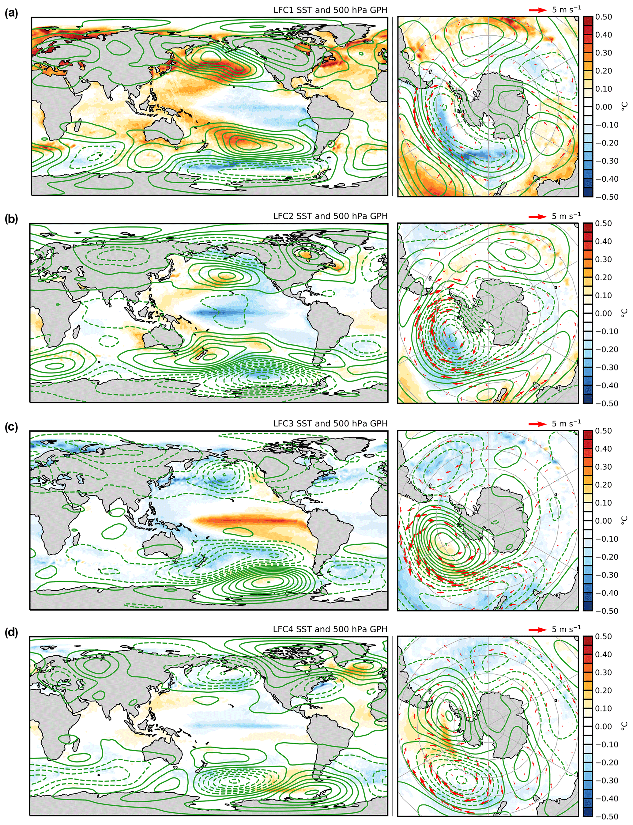
Figure 6 Mechanisms for low-frequency variability in Antarctic sea ice concentration. Regression of annual-mean sea surface temperature (color shading) and 500 hPa geopotential height field (green lines) onto the (a) first, (b) second, (c) third, and (d) fourth LFCs (10-year cutoff, five EOFs retained) in annual-mean Southern Hemisphere sea ice concentration from 1979 to 2022. The spacing for the 500 hPa geopotential height anomaly field is from −200 to 200 m at 20 m intervals. The left column shows the global domain, and the right column shows the Southern Ocean domain. The red vectors on the panels in the right column denote the regression of annual-mean near-surface wind anomalies onto each LFC.

Each LFC exhibits a distinct spatial pattern of SST and 500 hPa GPH that is largely associated with Pacific and Southern Ocean climate variability (Fig. 6). The SST pattern associated with LFC1 is reminiscent of the Interdecadal Pacific Oscillation (IPO), with a tripole-like SST pattern throughout the entire Pacific basin (Fig. 6a, left). This result supports Meehl et al. (2016), who argued that the phase of the IPO is a key source of the long-term positive trend in Antarctic sea ice concentration from 2000 to 2014. However, the LFC1 SST pattern also resembles the observed SST trend over this time period, which climate models struggle to reproduce (Wills et al., 2022), raising the possibility that LFC1 could represent a transient response to anthropogenic forcing. The pattern of 500 hPa GPH associated with LFC1 exhibits strong positive values in the extratropics and negative values over the Southern Ocean (Fig. 6a, right), reminiscent of a Rossby wave train emanating from the tropical Pacific. In the Southern Ocean, LFC1 is associated with large-scale surface cooling and negative 500 hPa GPH values in the Pacific sector, indicating a strengthening of the westerlies from the late 1970s (Fig. 6a, right). This is consistent with previous studies which have argued that surface cooling is linked to strengthening westerlies as a result of enhanced northward Ekman heat transport (e.g., Hall and Visbeck, 2002).

The other LFCs exhibit various patterns of tropical Pacific variability, with little influence from the Atlantic basin (Fig. 6b–d, left). LFC2, for instance, has an SST pattern reminiscent of the central Pacific ENSO, with negative SST anomalies centered in the equatorial Pacific basin (Fig. 6b, left). The SST pattern associated with LFC2 also has structure throughout the Pacific basin and somewhat resembles the North Pacific Gyre Oscillation (NPGO), which is known to influence and be influenced by the central Pacific ENSO (Di Lorenzo et al., 2010). However, it is important to note that LFC2 is not purely the central Pacific ENSO and contains higher-frequency variability associated with atmospheric circulation in the Southern Ocean. For instance, LFC2 has strong negative 500 hPa GPH anomalies and negative surface temperature anomalies in the Ross Sea (Fig. 6b, right). This pattern of atmospheric circulation closely resembles the pattern of atmospheric circulation associated with the SAM (Fogt and Marshall, 2020), with negative 500 hPa GPH anomalies throughout the polar cap. This is also evident in LFC2, which exhibits strong positive values in the late 1990s, consistent with well-documented strong SAM and central Pacific ENSO events (e.g., Marshall, 2003; Fogt and Marshall, 2020). The SST and 500 hPa GPH pattern of LFC2 is consistent with well-known short-term Southern Ocean Ekman dynamics and the SAM, whereby wind anomalies lead to surface temperature anomalies through anomalies in northward Ekman heat transport (e.g., Kostov et al., 2017) and Ekman pumping or suction.

The SST pattern associated with LFC3 is similar to the eastern Pacific ENSO, with an elongated SST structure centered on the Equator that extends across the Pacific basin (Fig. 6c, left). A pattern of positive SST anomalies in the Pacific (i.e., El Niño) favors strong cooling throughout much of the Southern Ocean (Fig. 6c, right). Here, a positive phase of LFC3 is associated with weaker winds in the Ross Sea and stronger winds in the Weddell and Scotia seas, as well as stronger meridional flow in the Amundsen and Bellingshausen seas. The structure of the surface winds favors strong meridional heat and moisture transport in the Ross Sea and in the eastern edge of the Bellingshausen Sea. However, these surface wind patterns would also cause strong patterns of Ekman pumping and suction that affect the vertical transfer of heat. Note that negative SST anomalies in the Pacific (i.e., La Niña) indicate strong surface warming in the Weddell and Scotia seas and weak surface warming in the Indian and West Pacific sectors (Fig. 6c).

Finally, the SST pattern associated with LFC4 also exhibits a weak signature in the tropical Pacific, with a narrow band of negative SST anomalies on the Equator in the central part of the Pacific basin (Fig. 6d, left). Interestingly, this SST pattern coincides with the ENSO region but does not exhibit the same degree of elongated SST structure as seen with LFC3 (compare Fig. 6c with d, left). LFC4 exhibits positive SST anomalies in the Amundsen and Bellingshausen seas, promoting sea ice melt (Fig. 6d, right), with weaker SST changes in other regions of the Antarctic. The SST and GPH height anomalies associated with LFC5 (the last LFC) are shown in Fig. A2. LFC5 exhibits a similar atmospheric circulation structure to the zonal wave three index, with strong meridional flow in the Ross and Weddell seas. LFC5 also exhibits little connection to SSTs elsewhere across the globe, except for small cooling in the central Pacific. This suggests that LFC5 represents higher-frequency atmospheric variability in the Southern Ocean, which is unique compared to LFC1–4.

In the next subsection, we re-examine how these modes of sea ice variability and the associated patterns of climate variability relate to periods of abrupt sea ice decline.

4.2 Context for periods of abrupt decline

In 2016, Antarctic sea ice concentration experienced an abrupt decline (Fig. 1a and c). While the 2016 decline in Antarctic SIA clearly stands out in the satellite record, there have been other periods of abrupt sea ice loss, as suggested by LFC3, such as in the late 1980s and throughout the middle to late 2000s. We now re-examine sea ice concentration anomalies associated with each LFC but focus on changes over periods of abrupt decline. These periods were identified as 4-year time periods where LFC3 transitioned from above 1 standard deviation to below 1 standard deviation. This resulted in two low-to-high (L–H) composites: 1989–1990 minus 1987–1988 and 2017–2018 minus 2015–2016. In the subsection below, we refer to each as event 1 and event 2, respectively.

Figure 7 shows the Antarctic sea ice concentration change for these two time periods in observations (Fig. 7a) and in each LFC (Fig. 7b–e). During event 1, negative sea ice concentration anomalies occurred throughout much of the Antarctic (Fig. 7a, left). However, positive sea ice concentration anomalies also occurred in the Weddell Sea, Indian sector, and parts of the Amundsen and Bellingshausen seas (Fig. 7a, left). During event 2, on the other hand, there was a similar negative sea ice concentration anomaly pattern but no corresponding positive sea ice concentration anomalies in the Weddell Sea and parts of the Amundsen and Bellingshausen seas (Fig. 7a, right). The same L–H composites for each LFC show that these slightly different sea ice concentration anomaly patterns, and therefore the different SIA declines, arise from LFC1. During event 1, LFC1 contributes large positive sea ice concentration anomalies throughout much of the Antarctic, while during event 2, LFC1 did not contribute to changes in sea ice concentration. Both LFC2 and LFC3 exhibit similar magnitudes of sea ice concentration change for event 1 and event 2, showing negative sea ice concentration anomalies in the Ross Sea from LFC2 (Fig. 7c) and throughout much of the Antarctic from LFC3 (Fig. 7d). This suggests that one reason event 1 was not as anomalous as event 2 was because of counteracting modes of tropical variability (LFC1 and LFC3), which prevented large negative sea ice concentration anomalies from emerging in the Weddell Sea and Amundsen and Bellingshausen seas.

To better understand the processes responsible for the different sea ice concentration anomalies for these two time periods, we examine components of a Southern Ocean mixed-layer temperature T_m budget (assumed to be equal to the SST). We assume SST anomalies are related to sea ice concentration anomalies. Following Pellichero et al. (2017), the rate of change of T_m can be expressed in terms of air–sea fluxes, horizontal advective fluxes (geostrophic, ageostrophic, and Ekman), vertical entrainment at the base of the mixed-layer h_m, and diffusive processes:

$$\begin{array}{}\text{(1)}& {\displaystyle \frac{\partial T_{\mathrm{m}}}{\partial t}}\approx {\displaystyle \frac{Q_{\mathrm{s}}}{{\mathit{\rho }}_{\mathrm{0}}{c}_p{h}_{\mathrm{m}}}}-{\mathit{u}}_{\mathrm{m}}\cdot \mathrm{\nabla }{T}_{\mathrm{m}}-w_{\mathrm{e}}{\displaystyle \frac{\mathrm{\Delta }T}{h_{\mathrm{m}}}}+\mathit{\kappa }{\displaystyle \frac{{\partial }^{\mathrm{2}}{T}_{\mathrm{m}}}{\partial z^{\mathrm{2}}}},\end{array}$$

where Q_s is the net surface heat flux (positive downwards) into the mixed layer, ρ₀ is a reference density of seawater, c_p is the specific heat of seawater, u_m is the mixed-layer averaged horizontal velocity (including geostrophic and Ekman components), w_e is the entrainment velocity associated with a variable mixed-layer depth, ΔT corresponds to the temperature differences across the base of the mixed layer, and κ is the vertical turbulent diffusion coefficient at the base of the mixed layer. The entrainment velocity w_e can be calculated from the rate of change in h_m following Ren and Riser (2009):

$$\begin{array}{}\text{(2)}& w_{\mathrm{e}}={\displaystyle \frac{\partial h_{\mathrm{m}}}{\partial t}}.\end{array}$$

It is possible to explicitly calculate each term in Eq. (1) and to assess their contribution to temperature changes in events 1 and 2. However, this is difficult with existing data products, particularly for early parts of the satellite record, and it is not the primary focus of this study. As noted by Tamsitt et al. (2016) and Pellichero et al. (2017), large uncertainties arise for a number of terms in Eq. (1) when using reanalysis products, making it difficult to close the temperature budget without taking a zonal average. Furthermore, estimates of geostrophic velocities and mesoscale eddies in the sea ice zone are weakly constrained and difficult to determine in observations. Instead, we plot the L–H composites of T_m, as well as various physical properties, such as the net surface heat flux, zonal-wind stress, and ocean mixed-layer depth, which contribute to components of Eq. (1). We assume that Ekman transport is the dominant contributor to the advection term in Eq. (1), particularly at scales much larger than the ocean mesoscale. The key changes in these composite properties are discussed below. However, we acknowledge that there may be significant contributions to mixed-layer temperature changes that arise from other terms, such as the vertical temperature difference across the base of the mixed layer, the turbulent diffusivity, and geostrophic velocities. We also acknowledge that the mixed-layer depth is poorly constrained in the Southern Ocean and may result in biased interpretations when compared to mixed-layer depth calculations from the ARGO-based gridded product.

Both abrupt decline events are associated with positive SST anomalies in the Scotia Sea (north of the Weddell Sea), but event 2 exhibits more circumpolar warming when compared to event 1, which exhibits negative SST anomalies in the Ross Sea and West Pacific and Indian sectors (Fig. 8a). Differences in Southern Ocean circumpolar westerlies likely explain the different characteristics of these two abrupt sea ice decline periods (Fig. 8). In the Southern Ocean, for event 1, the SST anomalies are somewhat correlated with surface heat flux anomalies (Fig. 8b, left), while for event 2, the SST anomalies are less correlated with surface heat flux anomalies (Fig. 8b, right). In fact, event 2 is mostly related to weakened circumpolar westerlies in the Southern Ocean (Fig. 8c, right), which would cause an anomalous convergence of heat along the margins of the sea ice edge due to weaker northward Ekman transport. Furthermore, the ocean mixed-layer depth shoaled more broadly and to a greater extent in event 2 as compared to the mixed-layer depth change that occurred during event 1 (Fig. 8d). This larger shoaling would amplify the warming associated with surface heat flux and Ekman changes, and it would cause mixed-layer warming through reduced entertainment of cold waters, as noted in Eq. (1). The anomalous shoaling of the ocean mixed layer is consistent with a reduction in westerly wind strength (Wilson et al., 2023).

Indeed, the different changes between event 1 and event 2 can be inferred from Figs. 2 and 6. When LFC1 is in a positive phase, meaning there are strong positive sea ice concentration anomalies throughout much of the Antarctic (Fig. 2a), near-surface winds strengthen, and there is surface cooling (Fig. 6a, right). This cooling counteracts warming due the weakening of the near-surface zonal winds that is associated with LFC3 and allows for larger meridional flow that can lead to substantial regional sea ice concentration variations (Fig. 6c, right). Figure 8 shows that event 1 – which is a combination of LFC1 and LFC3 – exhibits little-to-no weakening of the circumpolar westerlies, while event 2 – which is mostly LFC3 – exhibits strong weakening of the circumpolar westerlies. The counteracting of LFC1 and LFC3 in event 1 prevents both reduced northward Ekman heat transport and a shoaling of the ocean mixed layer, which supports near-circumpolar warming throughout the Southern Ocean and likely circumpolar sea ice loss. However, additional work is required to link SST anomalies to sea ice concentration anomalies as it is clear some of the strongest negative sea ice concentration anomalies do not coincide with the strongest positive SST anomalies.

Figure 7 Periods of abrupt Antarctic sea ice decline. Changes in annual-mean Antarctic sea ice concentration from (a) observations and from (b–e) each LFP component for (left) 1987–1990 and (right) 2015–2018. Changes are calculated as differences between the first 2 years and last 2 years of each period. Event 1 is 1989–1990 minus 1987–1988, and event 2 is 2017–2018 minus 2015–2016. These periods were identified as 4-year time periods where LFC3 transitioned from above 1 standard deviation to below 1 standard deviation.

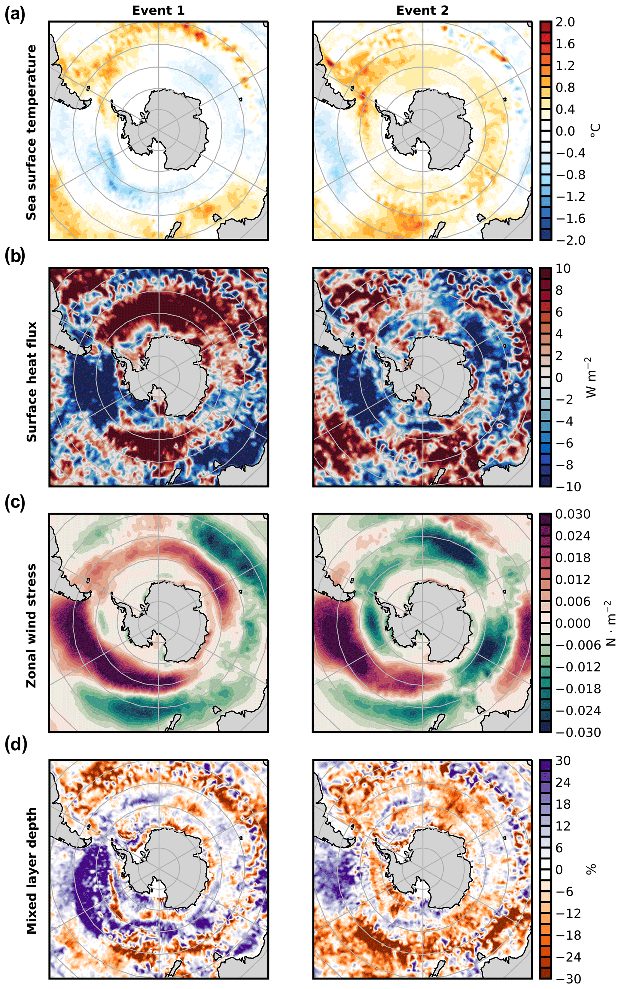
Figure 8 Processes associated with periods of abrupt Antarctic sea ice decline. Changes in annual-mean (a) sea surface temperature, (b) net surface heat flux, (c) zonal wind stress, and (d) ocean mixed-layer depth for (left) 1987–1990 and (right) 2015–2018. The ocean mixed-layer depth anomalies are normalized by the climatology. Changes are calculated as differences between the last 2 years and first 2 years of each period. Event 1 is 1989–1990 minus 1987–1988, and event 2 is 2017–2018 minus 2015–2016.

5 Discussion and conclusions

The recent decline in Antarctic sea ice, which occurred after a gradual, long-term increase, demonstrates that, under certain conditions, Antarctic sea ice can be susceptible to rapid changes. It is well understood that Antarctic sea ice exhibits substantial interannual-to-decadal variability, but the precise mechanisms responsible for this variability and how these mechanisms manifest spatially and temporally in the observational record have remained unclear. In this paper, we used a statistical method (i.e., LFCA; Wills et al., 2018; Schneider and Held, 2001) to identify patterns and distinct modes of low-frequency variability in observed Antarctic sea ice concentration. The leading mode represents the large-scale, gradual expansion of Antarctic sea ice. This mode accounts for approximately all of the observed trends in Antarctic sea ice concentration and long-term trends in regional and total Antarctic SIA. The next three modes represent higher-frequency sea ice variability. The second mode (LFC2) accounts for most of the sea ice variability in the Ross Sea and contributes to some sea ice variability in the Weddell Sea. The third mode (LFC3) accounts for the abrupt decline in sea ice concentration around 2016 and captures most of the SIA variability in the Weddell Sea and for pan-Antarctic SIA. The fourth mode (LFC4) accounts for sea ice variability mainly in the Amundsen and Bellingshausen seas.

We identified large-scale atmospheric and oceanic mechanisms associated with each mode, including processes that are related to the gradual expansion of and abrupt decline in Antarctic sea ice concentration. All LFCs are influenced to some degree by tropical Pacific variability, with little influence from the Atlantic basin. The SST pattern associated with LFC1 is reminiscent of the IPO, featuring a tripole-like SST pattern across the Pacific basin. This is consistent with Meehl et al. (2016), who argued that observed Antarctic sea ice expansion is related to the IPO phase. The spatial pattern of SST associated with LFC1 also resembles the observed trend in SST that climate models struggle to reproduce (e.g., Wills et al., 2022), meaning biases in Antarctic sea ice and large-scale SST trends are likely related. However, it is still unclear to what extent large-scale SST trends are the cause of or result of Southern Ocean trends. Dong et al. (2022a) showed that Southern Ocean cooling can cause a two-way teleconnection that results in a similar SST pattern to observed trends. This means that other sources of Southern Ocean cooling, such as increased surface freshening (Pauling et al., 2016; Sadai et al., 2020; Haumann et al., 2020; Dong et al., 2022b), might also impact large-scale SST trends. Still, the anomalous circulation associated with LFC1 indicates a strengthening of the circumpolar westerlies and some surface cooling throughout the Southern Ocean. This is also consistent with recent work that has argued that near-surface wind trends are a key ingredient of observed Antarctic sea ice expansion and Southern Ocean cooling (e.g., Blanchard-Wrigglesworth et al., 2021; Sun and Eisenman, 2021).

The other LFCs are related to higher-frequency Pacific variability. LFC2 is related to the central Pacific ENSO and SAM, with a strong atmospheric circulation pattern centered in the Ross Sea and Weddell Sea. LFC3 – the mode that accounts for the abrupt decline in sea ice around 2016 – has an SST pattern reminiscent of the eastern Pacific ENSO. This mode favors strong surface warming in and around the Weddell Sea when the eastern Pacific ENSO is in a negative phase and strong surface cooling when the eastern Pacific ENSO is in a positive phase. This mode also contains a signature of Amundsen Sea low variability, with a strong pattern of atmospheric circulation near the Amundsen and Ross seas (Raphael et al., 2016). We showed that LFC3 accounts for the 2016 decline event through a weakening of circumpolar westerlies, which favors weaker northward Ekman heat transport and shoaling of the ocean mixed-layer depth, both of which would cause warming and sea ice melt. We also showed that the abrupt sea ice decline event in 2016 was unique from other periods of abrupt sea ice decline identified by LFC3 (e.g., 1989–1990) because of compensating effects from LFC1. Finally, LFC4, which is more localized to the Amundsen and Bellingshausen seas, is weakly related to other tropical variability in the central equatorial Pacific. Interestingly, this mode of Pacific SST variability occurs in a similar region that other studies have argued strongly impacts the Amundsen and Bellingshausen seas (e.g., Steig et al., 2012; Dutrieux et al., 2014; Holland et al., 2019). These studies have argued that increased ice shelf melt in the Amundsen and Bellingshausen seas arises from increased poleward ocean heat transport driven by central equatorial Pacific climate variability. Our work suggests that this mode also impacts Antarctic sea ice and is distinct from the central Pacific ENSO.

While these results demonstrate the utility of LFCA for interpreting interannual-to-decadal sea ice variability, here we focused only on annual-mean Antarctic sea ice. Antarctic sea ice exhibits strong seasonality, with larger positive sea ice trends in the austral autumn and enhanced sea ice variability in the austral winter (Holland, 2014). Recent work has also shown that the seasonality of near-surface winds and mixed-layer depth in conjunction with surface heating can produce large and abrupt circumpolar surface warming in the Southern Ocean (Wilson et al., 2023), which could also cause abrupt sea ice changes. However, this study focused on the region of the Southern Ocean that is free of sea ice, making it difficult to compare these two studies. Other studies have indeed shown that seasonal changes in ENSO and other modes of climate variability can also exert strong control over sea ice changes (e.g., Stuecker et al., 2017; Schlosser et al., 2018). In particular, Stuecker et al. (2017) argued that the persistence of positive SST anomalies in the Ross, Amundsen, and Bellingshausen seas from a positive ENSO phase in December–February contributed to the abrupt decline in Antarctic sea ice in 2016. Examining sources of low-frequency Antarctic sea ice variability on seasonal timescales might improve the mechanistic interpretation of the observational record. Such work might also explain why other periods with large ENSO events, such as 1997–1998, did not result in large Antarctic sea ice changes. Our work suggests that the flavor of ENSO can result in different Antarctic sea ice concentration changes, and further examination on seasonal timescales might also reveal unique sea ice changes for different ENSO events.

Although these results do not provide a full mechanistic pathway to explain abrupt Antarctic sea ice changes, the results do provide context for periods of abrupt decline that might inform climate model experiments that provide a more mechanistic understanding. Our results suggest that SST variability in different regions of the Pacific can result in regionally distinct Antarctic sea ice concentration anomalies that sometimes counteract each other. These results could inform so-called “pacemaker” experiments (e.g., Kosaka and Xie, 2013), where SSTs are relaxed to observed values to isolate key regions of influence over climate variables. Performing these experiments over various regional domains of the Pacific might demonstrate the importance of phasing in Pacific climate variability in contributing to abrupt sea ice changes. Such experiments might also better elucidate the mechanisms underpinning Antarctic sea ice variability and help to clarify why certain periods, such as the late 1980s or 1990s, did not result in widespread and abrupt sea ice loss. This work might also help to clarify whether or not observed Antarctic sea ice has experienced a regime change (e.g., Raphael and Handcock, 2022; Fogt et al., 2022) as multiple simulations can be performed, providing context for internal variability.

In summary, LFCA can identify modes of sea ice variability associated with both the gradual long-term increase and the sudden decrease in observed Antarctic sea ice. While LFCA has been used in other studies to isolate the forced response (Wills et al., 2020; Dörr et al., 2023), the large interannual-to-decadal variability in Antarctic sea ice makes this analysis inconclusive about the sign or pattern of Antarctic sea ice response to anthropogenic forcing over the historical period. Still, this method and framework thus open up other avenues of sea ice research. For example, applying this method to climate models might help identify mechanisms responsible for the large discrepancies in Antarctic sea ice trends between climate models and observations over the satellite record (e.g., Purich et al., 2016; Rosenblum and Eisenman, 2017; Roach et al., 2020). Our results show that the SST pattern associated with LFC1 – which captures the long-term expansion of Antarctic sea ice – resembles the SST trend bias in state-of-the-art climate models (see Fig. 1 in Wills et al., 2022), which suggests that biases in the SST and Antarctic sea ice trends of climate models are related to the same physical processes. Our results also highlight mechanisms impacting short-term sea ice changes. The large influence of ENSO on abrupt sea ice changes suggests that, as ENSO transitions from its negative phase (2020–2022) to its positive phase, Antarctic sea ice cover might increase, potentially offsetting the anomalous decline seen since 2016. However, our analysis indicates that the impact of ENSO on Antarctic sea ice depends on whether ENSO manifests more in the central or eastern Pacific, suggesting it will be crucial to monitor regional Pacific SST variability for short-term predictions of Antarctic sea ice changes.

Appendix A

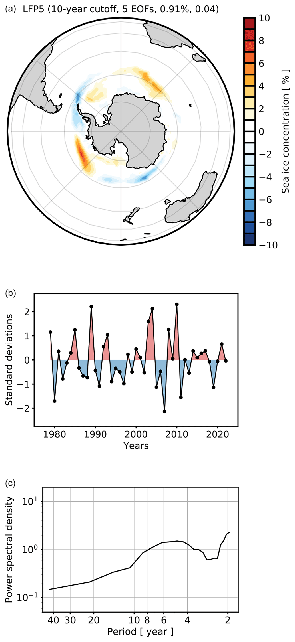
Figure A1 The additional low-frequency component and pattern. Fifth (a) low-frequency pattern (LFP), (b) low-frequency component (LFC), and (c) power spectra density of the LFC using a 10-year cutoff and retaining the five leading EOFs with annual-mean Antarctic sea ice concentration anomalies from 1979 to 2022. Power spectra are computed with multitaper spectral analysis (Percival and Walden, 1993). The fraction of explained low-frequency variance (in %) and the ratio r of low-frequency variance to total variance is given for each pattern in the titles of the top panels.

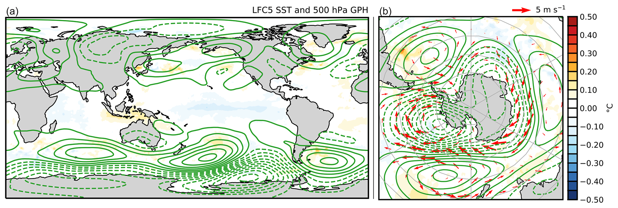
Figure A2 Mechanisms for additional low-frequency variability in Antarctic sea ice concentration. Regression of annual-mean sea surface temperature (color shading) and 500 hPa geopotential height field (green lines) onto the fifth LFC (10-year cutoff, five EOFs retained) in annual-mean Southern Hemisphere sea ice concentration from 1979 to 2022. The spacing for the 500 hPa geopotential height anomaly field is from −200 to 200 m at 20 m intervals. The left column shows the global domain, and the right column shows the Southern Ocean domain. The red vectors on the panels in the right column denote the regression of annual-mean near-surface wind anomalies onto each LFC.