the Creative Commons Attribution 4.0 License.
the Creative Commons Attribution 4.0 License.
 | 26 Apr 2024
Snow depth in high-resolution regional climate model simulations over southern Germany – suitable for extremes and impact-related research?
Benjamin Poschlod
Anne Sophie Daloz
Snow dynamics play a critical role in the climate system, as they affect the water cycle, ecosystems, and society. In climate modelling, the representation of the amount and extent of snow on the land surface is crucial for simulating the mass and energy balance of the climate system. Here, we evaluate simulations of daily snow depths against 83 station observations in southern Germany in an elevation range of 150 to 1000 m over the time period 1987–2018. Two simulations stem from high-resolution regional climate models – the Weather Research & Forecasting (WRF) model at 1.5 km resolution and the COnsortium for Small scale MOdelling model in CLimate Mode (COSMO-CLM; abbreviated to CCLM hereafter) at 3 km resolution. Additionally, the hydrometeorological snow model Alpine MUltiscale Numerical Distributed Simulation ENgine (AMUNDSEN) is run at point scale at the locations of the climate stations, based on the atmospheric output of CCLM. To complement the comparison, the ERA5-Land dataset (9 km), a state-of-the-art reanalysis land-surface product, is also compared. All four simulations are driven by the atmospheric boundary conditions of ERA5.
Due to an overestimation of the snow albedo, the WRF simulation features a cold bias of 1.2 °C, leading to the slight overestimation of the snow depth in low-lying areas, whereas the snow depth is underestimated at snow-rich stations. The number of snow days (days with a snow depth above 1 cm) is reproduced well. The WRF simulation can recreate extreme snow depths, i.e. annual maxima of the snow depth, their timings, and inter-station differences, and thereby shows the best performance of all models.
The CCLM reproduces the climatic conditions with very low bias and error metrics. However, all snow-related assessments show a strong systematic underestimation, which we relate to deficiencies in the snow module of the land-surface model. When driving AMUNDSEN with the atmospheric output of the CCLM, the results show a slight tendency to overestimate snow depth and number of snow days, especially in the northern parts of the study area. Snow depth extremes are reproduced well.
For ERA5-Land (ERA5L), the coarser spatial resolution leads to larger differences between the model elevation and the station elevation, which contributes to a significant correlation of climatic biases with the elevation bias. In addition, the mean snow depth and number of snow days are strongly overestimated, with conditions that are too snowy in the late winter. Extreme snow depth conditions are reproduced well in the low-lying areas, whereas strong deviations occur with more complex topography.
In sum, due to the high spatial resolution of convection-permitting climate models, they show the potential to reproduce the winter climate (temperature and precipitation) in southern Germany. However, different sources of uncertainties, i.e. the spatial resolution, the snow albedo parametrisation, and other parametrisations within the snow model, prevent their further use in a straightforward manner for impact research. Hence, careful evaluation is needed before any impact-related interpretation of the simulations, such as in the context of climate change research.
- Article
(12648 KB) - Full-text XML
-
Supplement
(1593 KB) - BibTeX
- EndNote


The presence and absence of snow, as well as the snow depth, affect nature and humans on many different levels. The albedo of snow influences the radiation and energy balance of the surface (Warren, 2019). Its insulating effect protects plants and animals (Blume-Werry et al., 2016; Slatyer et al., 2022). In addition, snow cover affects the microbial structure of the soil (Gavazov et al., 2017). The seasonal cycle of snow cover duration and snow depth governs soil moisture dynamics (Qi et al., 2020) and the runoff regimes of rivers and streams (Girons Lopez et al., 2020; Poschlod et al., 2020a). Hence, the snow dynamics also affect the freshwater availability in large regions of the world (Barnett et al., 2005). Snow melt may also induce riverine floods (Berghuijs et al., 2019), often in combination with heavy rainfall (Poschlod et al., 2020b). Sufficient snow depths are needed for ski tourism (Steiger et al., 2017; Witting and Schmude, 2019) but are also expected by non-ski tourists during their winter holidays in the mountains (Bausch and Unseld, 2018). This also reflects the traditional and cultural meaning of snow cover, which manifests annually in discussions and expectations about a “white Christmas” in the Northern Hemisphere (Durre and Squires, 2015; Harley, 2003). Moreover, the presence of snow influences everyday life in terms of mobility. The usage of bikes or scooters is reported to significantly depend on snow depths (Mathew et al., 2019; Yang et al., 2018). Also, the alternatives (trains, cars, or planes) may be affected by high snow depths (Doll et al., 2014; Taszarek et al., 2020; Trinks et al., 2012). During extreme snow events, power shortages (Bednorz, 2013; Gerhold et al., 2019) or even collapses of roofs (Strasser, 2008b) occur, which is why building codes have to rely on the regional snow climate (Croce et al., 2018).
Due to these manifold effects, there is great interest in modelling snow dynamics and snow depths in order to be able to predict near-term snow conditions (Hammer, 2018) and to project future snow conditions (Frei et al., 2018). In general, snow models are used to simulate snow dynamics at different temporal and spatial scales. In global or regional earth-system model setups, snow dynamics are simulated coupled with atmospheric processes and other land-surface processes (Krinner et al., 2018). However, the spatial resolution of global and regional models is often not sufficient to represent complex terrain and the spatial variability of the land-surface (Mooney et al., 2022). Further, the simulated climate and snow dynamics show biases (Daloz et al., 2022). Often, for local to regional impact studies, the climatic biases are adjusted, in which case it is necessary to apply a method tailored to snow climates (e.g. Chen et al., 2018; Frei et al., 2018; Meyer et al., 2019). In the case of a simple univariate bias adjustment, the dependence between temperature and precipitation is not considered, which neglects the threshold effect of air temperature on the fractionation of precipitation into rain and snowfall (Meyer et al., 2019). Therefore, multivariate bias adjustment is recommended for hydrological impact modelling in regions with snow and rain dynamics (Chen et al., 2018; Meyer et al., 2019). In a next step, snow models are set up at higher resolution, driven by bias-adjusted climatic time series (Hanzer et al., 2018). Then, however, the simulated snow dynamics cannot feed back into the climate, which is why these simulations are called “offline”. Another possibility would be to directly adjust the biases of the snow parameter simulated by the climate model (Matiu and Hanzer, 2022).
Due to the advances in computational power, the spatial resolution of regional climate models (RCMs) has increased (Coppola et al., 2020). Kilometre-scale simulations are available for decade-long time spans. The high spatial resolution allows for a finer-scale representation of complex topography (Poschlod et al., 2018). Therefore, the effects of altitude on air temperature can be mapped in more detail, which better represents the fractionation into rain and snowfall as well as melting and accumulation processes. In addition, the higher resolution of land cover allows for more detailed simulation of the albedo, which in turn governs the energy balance (Winter et al., 2017). The high resolution also allows more processes to be included in the model chain. Snow drift due to wind and turbulence has been implemented in an offline setup (Vionnet et al., 2021), and it was also implemented online by coupling the RCM Weather Research and Forecasting (WRF) with the detailed snow model SNOWPACK (Sharma et al., 2023). Future work will aim at seamlessly implementing snow drift in WRF (Saigger et al., 2023).
Here, two high-resolution convection-permitting regional climate models are evaluated with station observations of daily snow depth in southern Germany for a 31-year period from 1987–2018. We analyse simulations of the WRF model (Skamarock et al., 2019) at 1.5 km resolution and the COnsortium for Small scale MOdelling (COSMO; Sørland et al., 2021) model in CLimate Mode (CLM) at 3 km resolution (hereafter abbreviated to CCLM). Both models are driven by atmospheric boundary conditions of ERA5 (Hersbach et al., 2020) at 31 km resolution. Moreover, the hydrometeorological snow model Alpine MUltiscale Numerical Distributed Simulation ENgine (AMUNDSEN) is run at the point scale of the climate stations driven by the atmospheric output of CCLM. In addition, the state-of-the-art land-surface reanalysis product ERA5-Land (9 km resolution; Muñoz-Sabater et al., 2021) is compared.
Such evaluation is important, as future projections of snow dynamics are often based on regional climate models (e.g. Frei et al., 2018; Räisänen, 2021). Even though mean snow depth and mean snow cover duration are expected to decrease due to higher temperatures, risks associated with snow dynamics might not (Musselman et al., 2018). While there are studies on climate model simulations and extreme snowfall (Quante et al., 2021; Sasai et al., 2019), we find no literature about extremes of snow depth dynamics within climate model simulations. Furthermore, there are studies evaluating regional climate models based on multi-decadal simulations, but these are at coarser spatial resolution (Daloz et al., 2022: 0.11°; Matiu and Hanzer, 2022: 0.11°; Steger et al., 2013: 0.22°). Recently, Monteiro and Morin (2023) compared the performance of multiple model systems with spatial resolutions ranging from 2.5 to 30 km over the European Alps. They found that main features of the snow cover, snow depth, and driving climatic conditions could be reproduced by the models but with increasing deviations at higher altitude. Lüthi et al. (2019) compared a 10-year simulation by COSMO at 2.2 km over Switzerland to interpolated observations. The mean seasonal cycle averaged over the country was reproduced well, but the model overestimated the mean snow water equivalent (SWE) at high altitudes.
In contrast to these existing high-resolution studies in Alpine terrain, we aim to assess snow conditions in southern Germany, mainly north of the Alpine crest, at a lower elevation range of between 150 to 1000 m. Even though the topography is less complex, snow dynamics still play a major role in this area, affecting natural systems (Poschlod et al., 2020a) and human systems (Strasser, 2008b; Doll et al., 2014; Frese and Blaß, 2011). Snow plays an important role in the tourism industry, where the sufficient presence of snow is important not only for ski tourists at higher altitudes but for all winter tourists (Bausch and Unseld, 2018; Witting et al., 2021). Due to the population density, there is high exposure to potential snow extremes. Within Germany, the study area covers a variety of snow load zones, which are used as the basis for the structural dimensioning of roofs (German Industry Norm DIN 1055-5; DIN, 2005). In the winter season of 2005/06, continuous snow cover conditions induced several roof collapses in the study area (Strasser, 2008b). During the recent winter (December 2023), snow depths above 40 cm in the study area (HND, 2024) led to a collapse in local and long-distance transport, power shortages, and damage to buildings and cars (Hagen and Mese, 2023; ARD, 2023).
Climate change already affects and will further alter snow dynamics and conditions (Dong and Menzel, 2020; Monteiro and Morin, 2023), which is why observation-based analyses are limited. Climate impact research and data users benefit from information at the local scale (Orr et al., 2021). In order to provide local information, coarse-resolution RCMs or even global circulation models have often been used to drive snow models at the local scale; however, these require bias adjustment, statistical downscaling and the de-coupling of the interactions of snow dynamics and climate, which induces additional uncertainties and limitations.
The “new generation” of high-resolution RCMs can potentially directly provide snow depth information based on their internal land-surface and snow modules. Hence, we see the need for a critical examination of what new-generation high-resolution RCMs are capable of in terms of snow dynamics and extremes. So, in addition to the evaluation of winter temperature and precipitation as well as mean winter snow depth and duration, which is also present in the above-mentioned studies, the study further aims to explore the capabilities of the high-resolution models to reproduce short-period snow conditions and extreme daily snow depths. The sample size required for this motivates a research setup where we select available multi-decadal high-resolution simulations (WRF, CCLM, and AMUNDSEN driven by CCLM) and compare them to the coarser-resolved product ERA5L. So, in sum, the study aims to evaluate (1) winter climate, (2) mean seasonal snow conditions, (3) short-duration snow conditions of relevance to the tourism sector, and (4) extreme snow depths in order to (5) explore the suitability of high-resolution climate models for impact-relevant snow research.
A comparative overview of the investigated simulation data is given in Table 1. The following sections describe the different model features and setups in detail. As a preliminary remark, we would like to point out that the historical genesis of the different model setups still governs the degree of complexity of the snow schemes. Single-layer snow schemes are common in the atmospheric community for numerical weather prediction (NWP) models and reanalyses (Arduini et al., 2019). Lee et al. (2023) give an overview of various snow parametrisations within nine land-surface models.
Table 1Overview of the different investigated model setups.
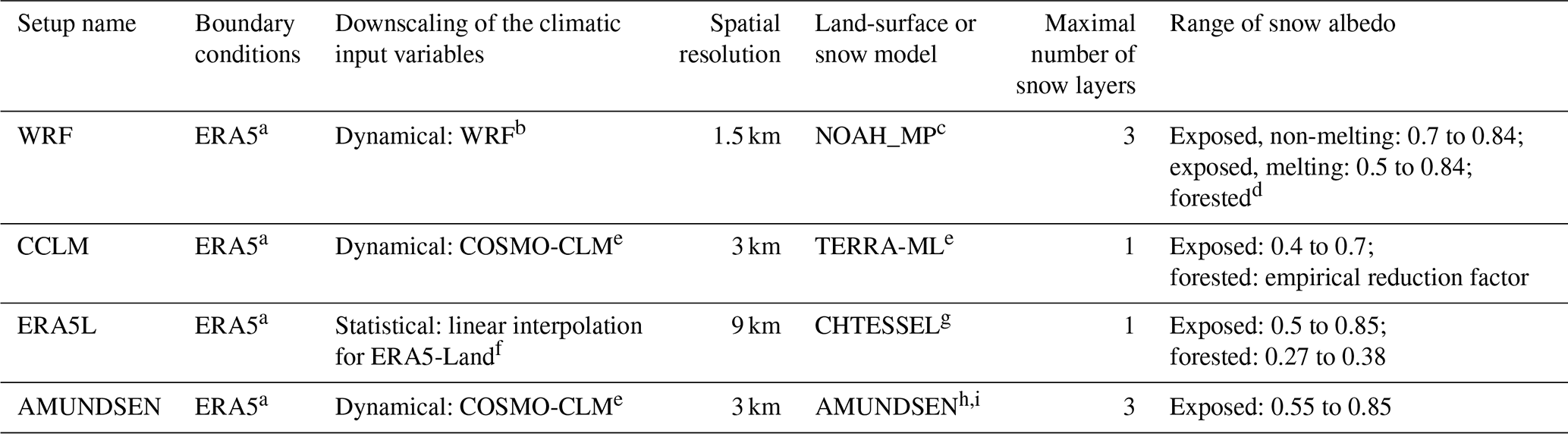
a Hersbach et al. (2020). b Skamarock et al. (2019). c Niu et al. (2011). d Niu and Yang (2004). e Doms et al. (2021). f Muñoz-Sabater et al. (2021). g ECMWF (2018), h Strasser (2008a). i Hanzer et al. (2018).
2.1 Regional climate models
Both RCMs are driven by the atmospheric-boundary conditions of the ERA5 reanalysis at 31 km resolution. The WRF simulations were carried out by Collier and Mölg (2020), where the setup is described in detail. Version 4.1 of WRF is run (Skamarock et al., 2019). The boundary conditions for ERA5 drive WRF at 7.5 km×7.5 km (one-way nesting), where spectral nudging is applied. The forcing at the lateral boundaries is updated at 3-hourly intervals. Increasing the spatial resolution by a factor of 5 within a second nesting step results in simulations at 1.5 km×1.5 km resolution, where convective processes are explicitly resolved. Collier and Mölg (2020) provide a general climatic evaluation with observational data. In order to simulate surface processes, WRF is run coupled with the land-surface scheme NOAH_MP (Niu et al., 2011). The physically based snow model in NOAH_MP features up to three snow layers, which are divided based on the simulated snow depth. In addition, four soil levels and a vegetation canopy layer are considered. Interception and burial of vegetation by snow is modelled following Niu and Yang (2004). The modelling of the density of newly fallen snow is dependent on the atmospheric temperature (Niu et al., 2011). The temperatures of the layers are calculated based on the energy balance for the snow and soil layers. Melting and freezing are assumed to occur above and below 0 °C, respectively. Mass transfer and energy transfer between layers are accounted for (Niu et al., 2011). In order to derive the snow depth, the density is assessed by representing snow metamorphism and compaction following Anderson (1976) and Sun et al. (1999). The snow surface albedo is calculated via the CLASS scheme (Verseghy, 1991), where the albedo of fresh snow is assumed to amount to 0.84. During melting conditions, the albedo exponentially decreases, with 0.5 used as the lower limit. Without melting conditions, 0.7 is assumed to be the lower limit. The snow albedo of forested areas is modelled as being dependent on the leaf and stem area index, accounting for snow interception, the loading and unloading of snow, and melting and refreezing (Niu and Yang, 2004). The ground surface albedo is calculated as an area-weighted average of the snow albedo and bare soil albedo (Niu et al., 2011). The WRF data are openly available (Collier, 2020).
COSMO was operationally applied as a weather forecasting model in Germany for over 20 years before being replaced by ICON (Rybka et al., 2022). For regional climate simulations, ICON-CLM was developed (Pham et al., 2021). Here, CCLM version 5-0-16 at 3 km resolution (Brienen et al., 2022) is still directly driven by the atmospheric conditions from ERA5, where the forcing is updated every hour (Rybka et al., 2022). The simulation domain covers Germany, the surrounding catchments, and parts of the Alps. Hence, the analysis domain is well within the simulation domain. The resolution of 3 km allows for the explicit simulation of deep convection, whereby shallow convection is parametrised. The land-surface model TERRA_ML is implemented in COSMO-CLM and represents soil, vegetation, and snow dynamics (Doms et al., 2021; Schulz and Vogel, 2020). It features multiple soil layers and either one interception reservoir or one snow reservoir on top of the soil, depending on the predicted temperature of the stored water. However, no canopy layer is implemented, which is common in NWP models but represents a major simplification for climate models (Schulz et al., 2016). Mass and energy fluxes between the atmosphere, the interception/snow reservoir, and the soil layers govern the temperature of the water in the reservoir. In the case of snow cover, the mean snow temperature is calculated based on the heat capacity of the snow, the atmospheric forcing at the snow surface, the heat flux to the soil, and melting processes (Doms et al., 2021). The density of fresh snow is assumed to range from 50 to 150 kg m−3 and is dependent on the temperature conditions. The empirical estimation of the mean snow density within the single snow layer includes two processes. Ageing, which is dependent on the snow temperature and time, increases the mean snow density of the reservoir, whereas newly fallen snow decreases the mean density. The range of densities is fixed between 50 and 400 kg m−3. Doms et al. (2021) claim that extreme snow depths cannot be properly accounted for by the model's concept. The range of possible snow depths is restricted to between 0.01 and 1.5 m. A time-dependent snow surface albedo is calculated, where the albedo covers the range between 0.4 for old snow and 0.7 for fresh snow (Doms et al., 2021). As the model features no canopy layer, no shading effects of vegetation are simulated. Instead, an empirical reduction factor for the snow albedo under vegetation is applied (Daloz et al., 2022). The CCLM data are available publicly (see https://esgf.dwd.de/projects/dwd-cps/, last access: 15 February 2024). However, albedo data were provided separately without quality checks (Susanne Brienen, German Weather Service, personal communication, 2023).
2.2 Land-surface model in ERA5-Land
ERA5-Land (ERA5L) directly derives its atmospheric forcing from the 10 m level of ERA5 at hourly resolution (Muñoz-Sabater et al., 2021). The 31 km resolution of ERA5 is linearly interpolated on the 9 km grid of ERA5-Land. The land-surface model Carbon Hydrology-Tiled ECMWF Scheme for Surface Exchanges over Land (CHTESSEL) then simulates energy and water cycles globally over land at hourly resolution. The snow scheme features one layer with a single temperature and density on top of the four-layered soil (ECMWF, 2018). The snow temperature is calculated based on the energy fluxes between the atmosphere and the snow skin, melting processes, and the basal heat flux. Snow temperature, mass, and density are used to derive the liquid water content within the snow pack. Interception of liquid water by the snow pack is accounted for. The snow density of fresh snow is modelled as being dependent on the atmospheric temperature and near-surface wind speed (Dutra et al., 2010). The snow density is assumed to change due to the overburden, thermal metamorphisms (Anderson, 1976), and compaction (Lynch-Stieglitz, 1994). The range of snow densities is restricted to between 50 and 450 kg m−3. The calculation of the snow surface albedo for exposed areas follows Verseghy (1991), with values ranging between 0.5 and 0.85. For forested areas, lower albedo values between 0.27 and 0.38 are applied following Moody et al. (2007), who based their calculations on remote-sensing products from MODIS. Further details of the land-surface scheme are provided by ECMWF (2018) and, especially for the snow scheme, by Dutra et al. (2010). The ERA5L data are openly available (https://cds.climate.copernicus.eu/cdsapp#!/dataset/reanalysis-era5-land?tab=overview, last access: 22 February 2024). Boussetta et al. (2021) present the new ECLand next-generation land-surface model, which introduces a multi-layer snow scheme following Arduini et al. (2019).
2.3 The hydroclimatological model AMUNDSEN
The hydroclimatological model AMUNDSEN has been developed to dynamically resolve the mass and energy balance of snow and ice in high-mountain regions (Strasser, 2008a; Hanzer et al., 2018). The model can be set up to be spatially distributed at high resolution (e.g. 10 to 100 m) and includes snow redistribution processes and a radiation scheme accounting for terrain slope and hill shading, for example (Hanzer et al., 2016). Here, we apply the model at point scale at the locations of the 83 climate stations. We use the CCLM output of hourly temperature, precipitation, wind speed, relative humidity, and short-wave radiation to drive openAMUNDSEN, the open model version implemented in Python (Warscher et al., 2021). No model-internal correction for precipitation undercatch is applied, as the climatological input stems from simulated precipitation by the CCLM. AMUNDSEN uses the wet-bulb temperature to differentiate between solid and liquid precipitation (Hanzer et al., 2018). The model features three snow layer categories, which are named “new snow”, “old snow”, and “firn”, depending on the snow density and age. The fresh snow density is calculated following Anderson (1976) and Jordan (1991) as being dependent on the air temperature. Compaction and metamorphism also follow empirical formulations by Anderson (1976) and Jordan (1991). Snow with a density above 200 kg m−3 is transferred to the old snow layer. The firn layer does not apply for the 83 locations, as no multi-year snow cover is simulated. Melting water in the snowpack may be retained by applying a parametrisation by Braun (1984). Snow albedo is parametrised as depending on the age of the snow and ranges between 0.55 and 0.85 for exposed surfaces following Hanzer et al. (2016). Snow-free albedo is set to 0.23, representing grassland, according to the climate conditions at the stations.
2.4 Study area and observational data
The study area covers large parts of southern Germany, with the boundaries given by the smallest simulation domain of the WRF model and the national borders. It includes a wide range of elevations of between roughly 100 and 3000 m above sea level (see Fig. 1a), which, therefore, have different snow dynamics. For the comparison to snow depth observations, we select 83 climate stations in the elevation range between 150 and 1000 m with less than 30 % missing data, which are operated by the German Weather Service (DWD, 2023). In order to assess the climatology, temperature and precipitation are analysed as well, where the precipitation is not corrected for undercatch. The mean annual temperatures of the locations range from 5.4 to 10.9 °C, and the mean annual precipitation covers the range between 580 and 1700 mm. The analysis period spans from November 1987 to April 2018, yielding 31 extended winter seasons. In this study, the extended winter season is defined as 6-month period from November to April. All analysis is carried out at daily resolution.
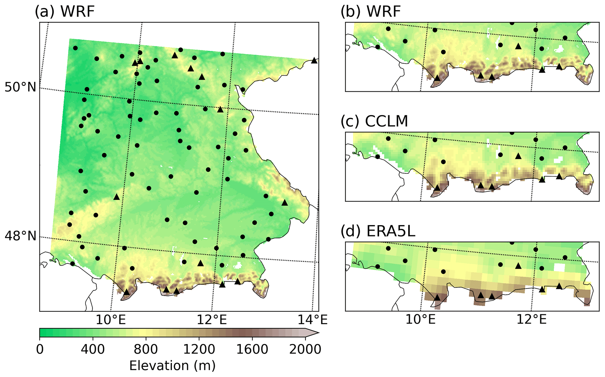
Figure 1Representation of elevation in the WRF (a). Lakes are masked out. The black markers show the 83 climate stations where the snow depth is observed. Dots (triangles) refer to stations with less (more) than 5 cm mean snow depth during the extended winter season. Zoomed displays of the complex terrain in the southern study area in WRF (b), CCLM (c), and ERA5-Land (d).
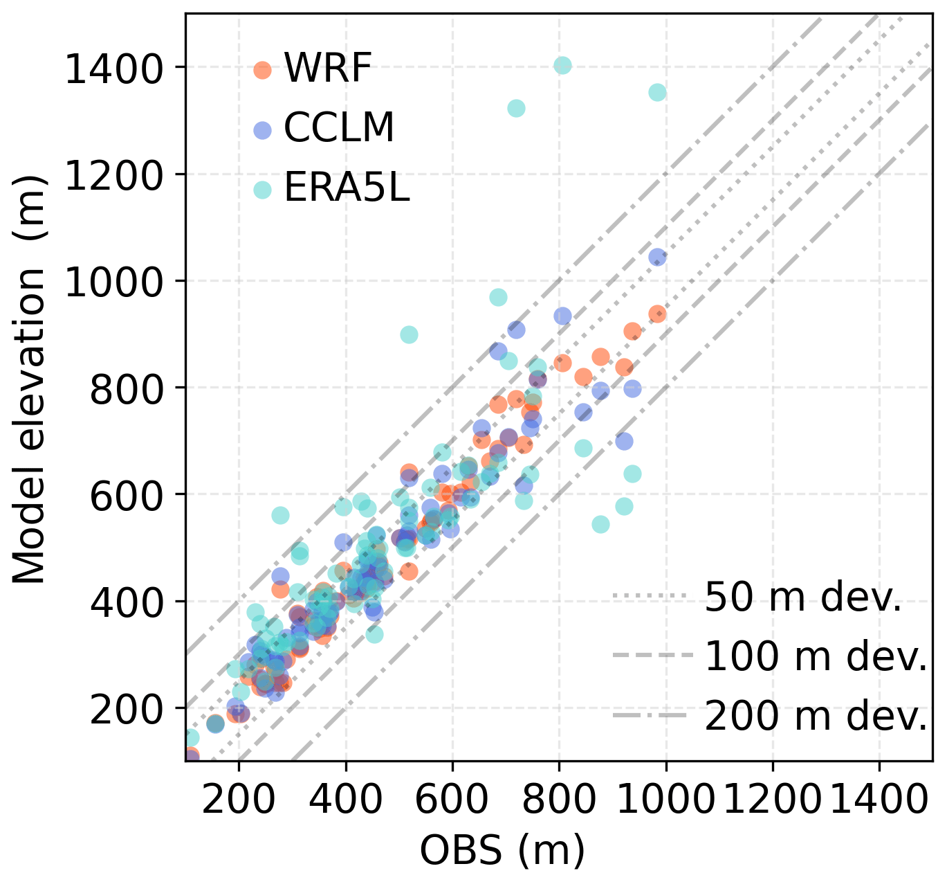
The comparison between the measured snow depth at a climate station and the simulated gridded snow depth is carried out via the nearest-neighbour approach. As the elevation within the gridded model varies according to the spatial resolution (Fig. 1b–d; see also Fig. S1 in the Supplement), the elevations of the climate station and the nearest model grid cell may differ. Figure 2 shows the degree to which a finer spatial resolution improves the representation of the altitude. The mean absolute deviation amounts to 24 m for WRF, 42 m for CCLM, and 93 m for ERA5L.
Due to the limited station density, we also include remote-sensing data for the model evaluation. Snow depth cannot be derived directly via optical remote sensing, but the snow cover fraction and the surface albedo can be derived. Therefore, we employ the daily snow cover and albedo from MODIS Terra at 0.05° resolution (Hall and Riggs, 2021; Schaaf and Wang, 2021), which is available for the period 2000–2018, although we only consider data qualified as “mixed”, “okay”, or better. Snow depth and SWE can be derived from microwave remote sensing by applying various retrieval algorithms (Tanniru and Ramsankaran, 2023; Tsang et al., 2022), but these result in considerable deviations for widely available products (Mortimer et al., 2020). New sensors and more-complex data-driven algorithms have shown the potential to improve these estimations (Daudt et al., 2023; Tsang et al., 2022), but are out of scope for this evaluation study.
2.5 Evaluation criteria
We evaluate the RCMs at the 83 climate stations and calculate the deviations for each winter season. The performance is assessed with four measures: the mean absolute error (MAE), the root-mean-square error (RMSE), the bias (BIAS) or percentage bias (PBIAS), and the Pearson rank correlation (r). For n observed values xobs and simulated values xsim, the measures are defined as follows:
In addition, we evaluate the simulations regarding the intensity and time-related measures of snow dynamics. Here, the mean winter snow depth refers to the mean snow depth over November to April. We define the number of “snow days” as the number of days with more than 1 cm snow depth across the whole year.
A “white Christmas” is defined as more than 1 cm snow depth on the 24, 25, and 26 December according to the German Weather Service (DWD, 2020). As this single 3 d period is rather selective, we also extend the same analysis to a 3 d moving window between November and April. In addition, we also assess the simulation of 5 d moving windows between December and February where snow depth is above 10 cm on each of the 5 d. This metric reflects the ability to do cross-country skiing (Vassiljev et al., 2010), as 5 d stays are typical for such vacations in the German mountain ranges (Hodeck and Hovemann, 2015). As these criteria lead to a binary classification for each moving window, the Matthews correlation coefficient (Matthews, 1975) is used as the evaluation metric. This considers true and false positives (TP and FP, respectively) as well as true and false negatives (TN and FN, respectively), which is why Luque et al. (2019) recommend it if classification success and errors are to be assessed. The MCC is defined as ranging between −1 and 1, where 0 indicates that the classification is as good as a random classifier.
In order to assess extreme conditions, we sample the annual maxima of snow depth. Based on this sampling, we fit the generalised extreme value (GEV) distribution, which can be applied to derive return levels of snow depth.
Here, μ is the location, σ is the scale, and ξ is the shape. The location parameter governs the centre of the distribution, the scale parameter corresponds to its spread, and the shape parameter governs the tail behaviour (Coles, 2001). We estimate these GEV parameters using a Markov chain Monte Carlo algorithm (Bocharov, 2022; Foreman-Mackey et al., 2013), generating confidence intervals at the 95 % level.
3.1 Biases in winter air temperature and precipitation
Precipitation and air temperature govern the snow dynamics to a large degree. A comparison of simulated and observed values of the winter temperature and precipitation is shown in Fig. 3. WRF systematically simulates winter temperatures that are too low, which has already been noted by Collier and Mölg (2020). Winter temperature is closely reproduced by CCLM with no bias (Fig. 3b). ERA5L has a slight cold bias, mostly due to single stations where the underestimation amounts to 4 °C (see Fig. 3c); this is a result of the elevation bias (Fig. 2). The WRF model slightly underestimates winter precipitation. However, as we do not correct the observed precipitation for undercatch, we would expect a slight overestimation from the RCMs. CCLM can reproduce winter precipitation with smaller errors, with the positive percentage bias of 9.5 % falling within the range of possible undercatch-induced deviations in southern Germany (Richter, 1995). The coarser-resolved ERA5L shows the biggest deviations, with a stronger positive deviation and the lowest rank correlation.
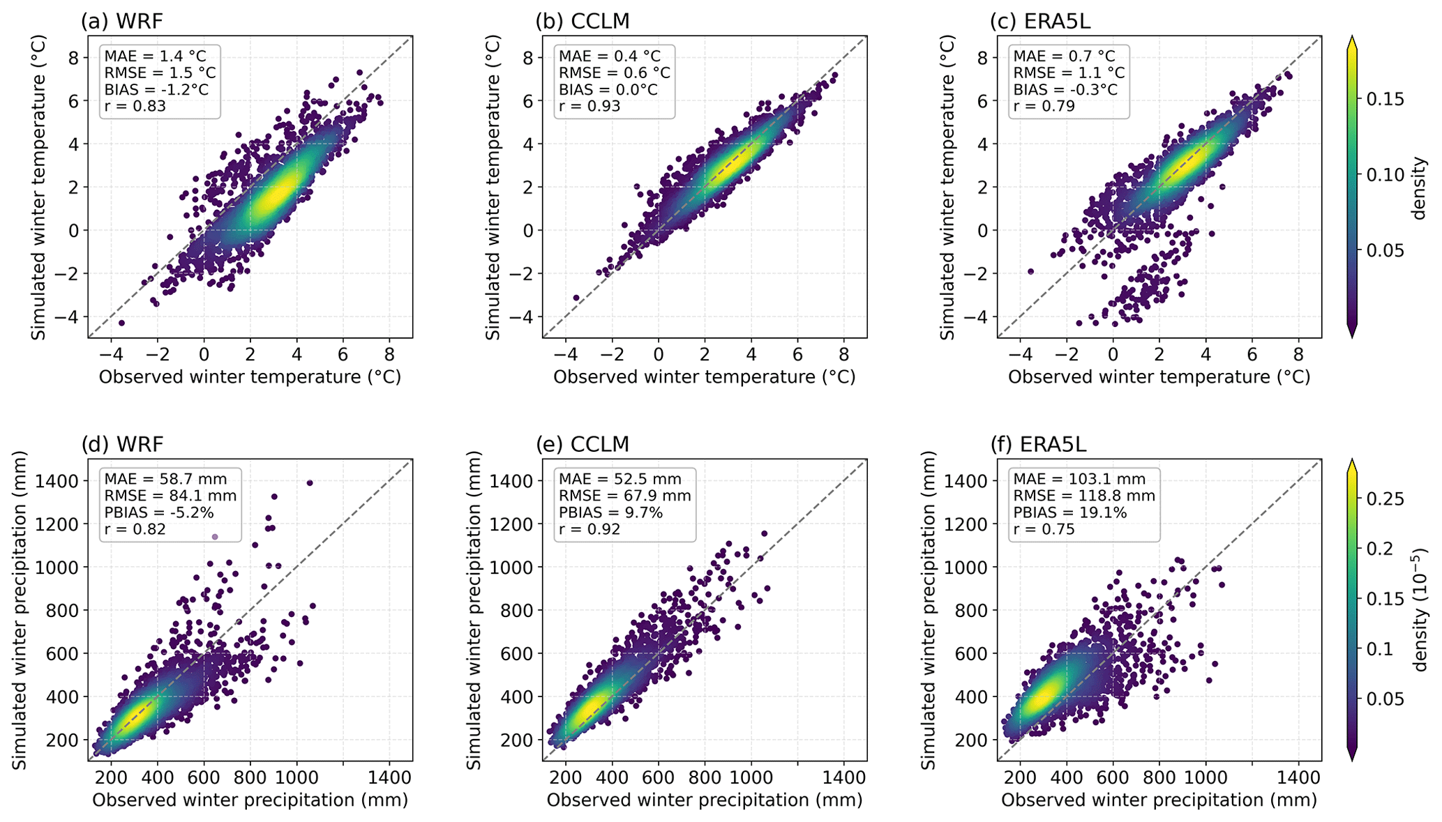
Figure 3Mean winter temperature (a–c) and precipitation (d–f) for each extended winter season and location in 1987–2018. Simulations by the WRF model (a, d), CCLM (b, e), and ERA5L (c, f) are compared to observations.
The differences between station elevation and mean grid-cell altitude also contribute to these biases. Elevation governs the temperature and also orographic precipitation effects (Warscher et al., 2019). Hence, Fig. 4a–f provide a comparison of the 31-year mean bias per location and the elevation difference. The Pearson rank correlations of elevation bias with temperature and precipitation bias are given in Table 2. For the biases in ERA5L, there is a clearly visible relationship (Fig. 4c and f) in which higher (lower) elevation bias leads to the overestimation (underestimation) of precipitation (r=0.49) and the underestimation (overestimation) of temperature (). For WRF and CCLM, no strong correlation is found; only a weak correlation of r=0.22 for the temperature bias in WRF is seen.
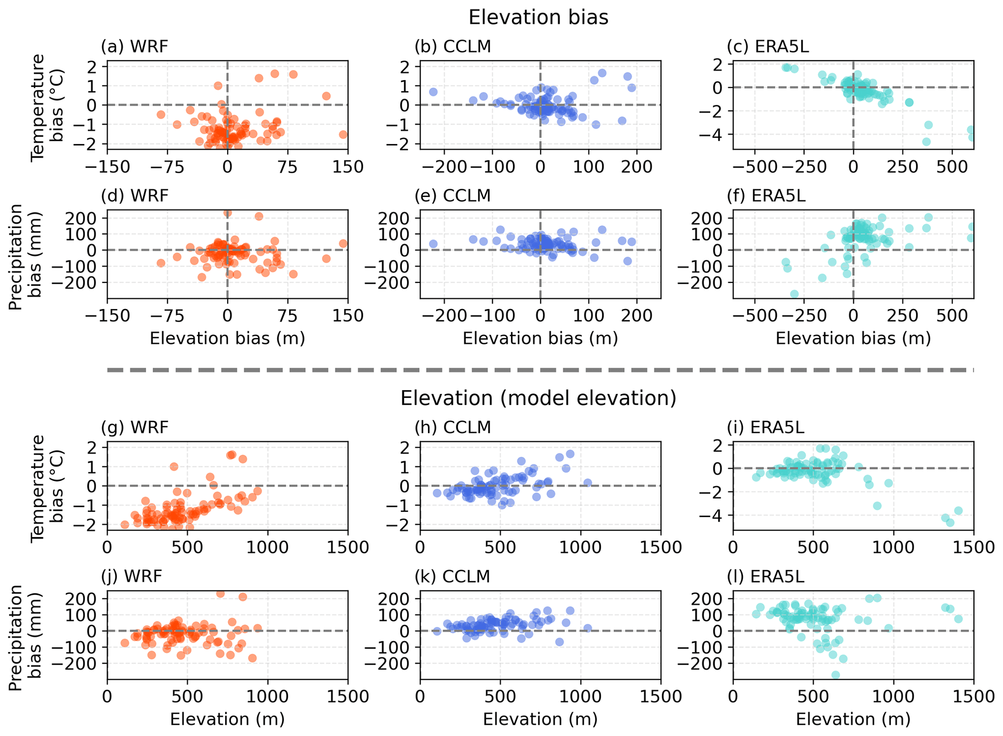
Figure 4Relationships of mean winter temperature and precipitation bias to the elevation bias (a–f) and the model elevation (g–l). Each location is averaged over 1987–2018. Elevation bias is calculated as model elevation minus station elevation.
Table 2Pearson rank correlations for elevation and climatological biases. Significant correlations at the 95 % (99 %) level are marked with one asterisk (two asterisks).
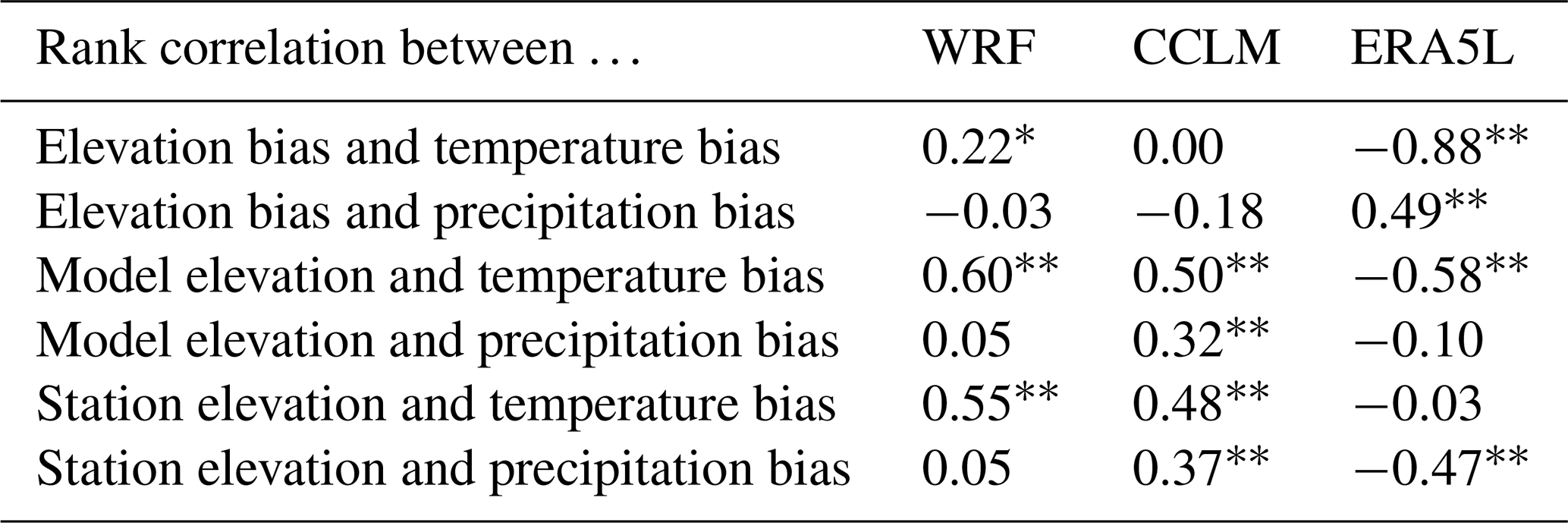
However, when compared with the absolute model elevation of each location, CCLM shows systematic deviations (Fig. 4h and k). Locations at higher (lower) model elevations tend to have temperatures that are too high (low) (r=0.50) and to be too wet (dry) (r=0.32). WRF shows higher temperature biases for higher elevations (Fig. 4g), yielding an overall rank correlation of r=0.60. The negative correlation between ERA5L model elevation and temperature bias () is governed by the locations at high and medium-high elevation (see the lower-right corner of Fig. 4i), as their temperature bias results from the high elevation bias (see Figs. 2 and 4c).
3.2 Snow depth evaluation
The evaluation of snow depth time series is challenging due to the long memory of the system and the error propagation over time. Furthermore, a proper evaluation depends on the intended use of the model data. If, for example, snow depth is simulated differently from an observation on the first day and it is correctly calculated that there is no change in snow depth for weeks, the error for the first day propagates for weeks, even though the model only simulated the accumulation differently on the first day.
To visualise this behaviour, we present the temporal evolution of snow depth during the winter season of 2005/06 at five selected locations (Fig. 5). In this season, continuous snow cover with several freezing and thawing cycles caused roof collapses and building evacuations in Bavaria (Strasser, 2008b). The time series show the temporal variability, the propagation of deviations, and the variability between models.
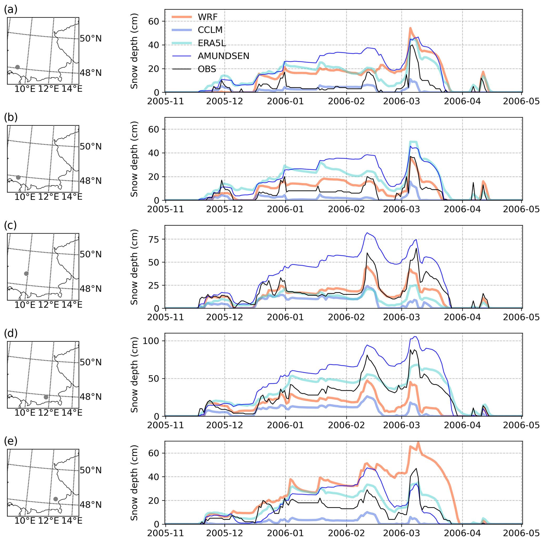
Figure 5Observed and simulated daily snow depth over the winter season 2005/06 at five locations.
In a further evaluation, 31 of these time series for 83 locations are condensed into different evaluation measures. We try to evaluate the simulations based on different impact-relevant measures.
The mean snow depth over the 31 winter half-years in 1987–2018 varies widely between the models (Fig. 6). The deviations are minor for the climate stations in flat areas with generally lower snow depths. WRF, ERA5L, and AMUNDSEN slightly overestimate snow depth in the flat areas, while CCLM slightly underestimates it. In the topographically complex northern regions of the low mountain range known as the Ore Mountains (in the far north-east), Thuringian Forest (north-central), and Rhön (to the north at 10° E), WRF, CCLM, and ERA5L underestimate snow depth (red dots in the north in Fig. 6a–c), whereas AMUNDSEN overestimates it. In the Alps, ERA5L largely overpredicts the snow depths, whereas CCLM heavily underestimates them. WRF underestimates them to a moderate degree and AMUNDSEN shows almost no bias. A general overview of simulated and observed snow depths against the elevation is provided in Fig. 7.
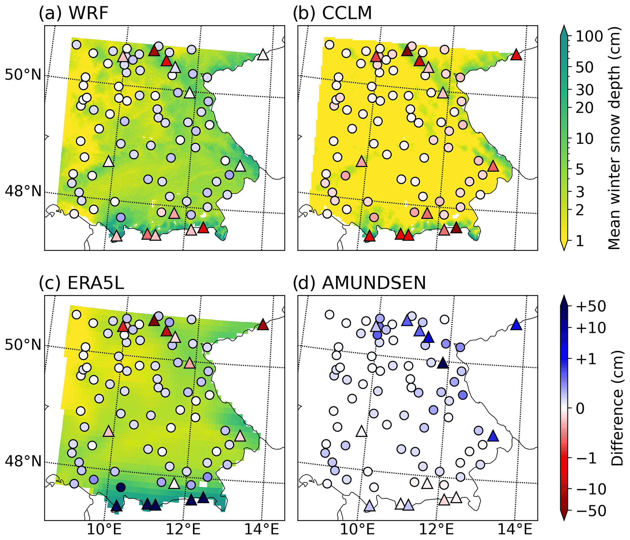
Figure 6Mean winter snow depth for 1987–2018 simulated by the WRF model (a), CCLM (b), ERA5L (c), and AMUNDSEN (d). The differences at the stations (coloured dots) are calculated as model minus observation. A red (blue) colour refers to underestimation (overestimation) by the model. Note the logarithmic colour scaling.
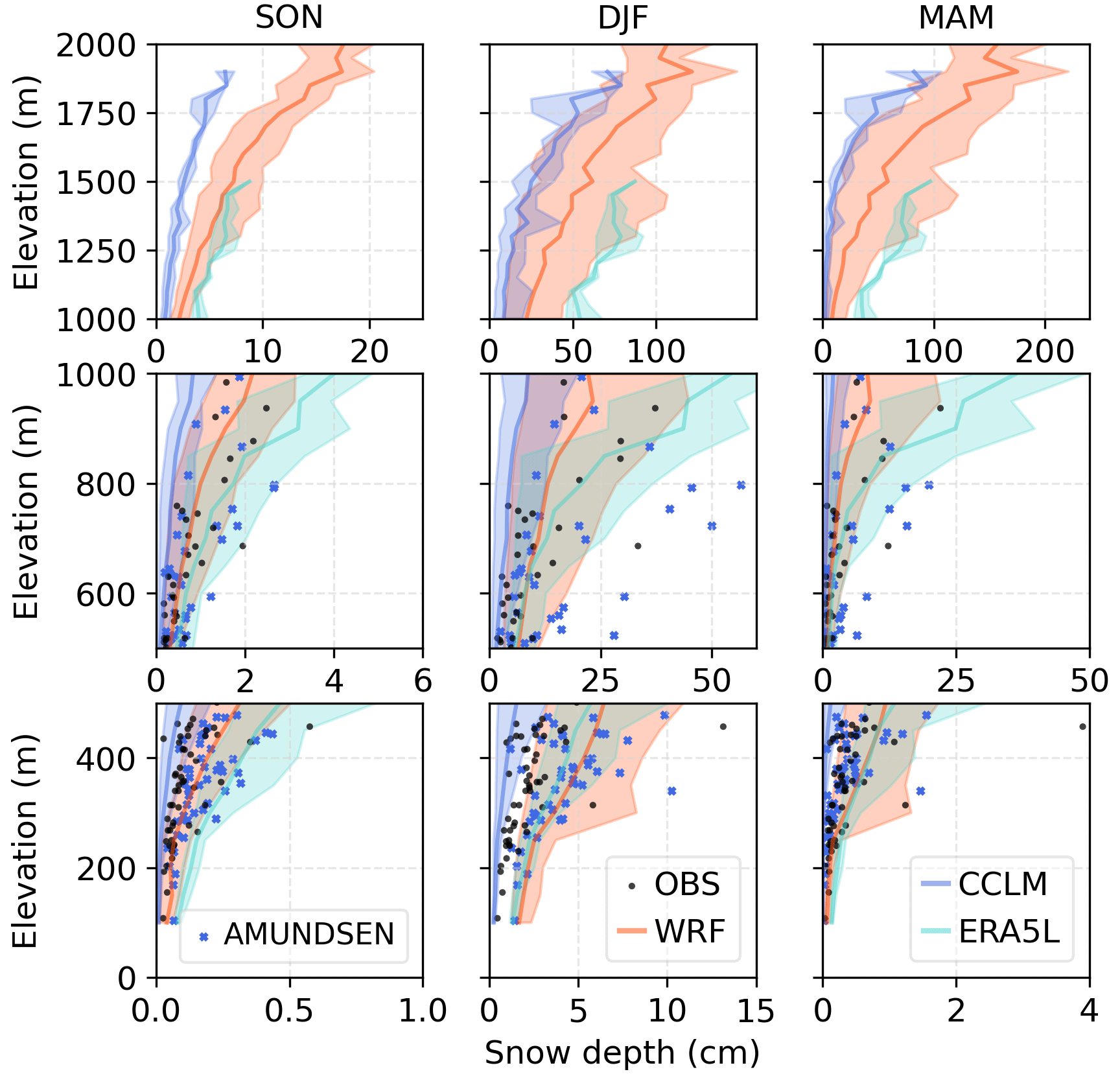
Figure 7Comparison of seasonal mean snow depths averaged over 1987–2018 for the whole range of elevations in the study area. The seasons considered are September–November (SON), December to February (DJF), and March to May (MAM). The shaded areas show the ranges for all grid cells at the respective elevation, and each line represents the median. Note the different x axis scaling for each plot. Also note that the elevations used in AMUNDSEN stem from CCLM, which is why they differ from the elevations of the observations.
When mean winter snow depth is assessed separately for each season and location, the WRF model shows low bias and errors (Fig. 8a and e). CCLM can give good metrics for stations that are less affected by snow (Fig. 8b), but it systematically underestimates snow depth at all stations. This negative bias of CCLM manifests itself in the fact that an overestimation of snow depth is not simulated for almost any station during any season (Fig. 8b and f; the magnitude of the bias is almost equal to the MAE). The ERA5L simulations have the highest bias and errors, with the biggest deviations seen over complex terrain (Fig. 8g). Especially during snow-rich seasons, strong overestimation is present for the Alpine stations, such that the stations in the low mountain ranges are heavily underestimated. AMUNDSEN shows the best overall rank correlation and the best reproduction of observed high-snow-depth seasons, although it has a tendency to overestimate.
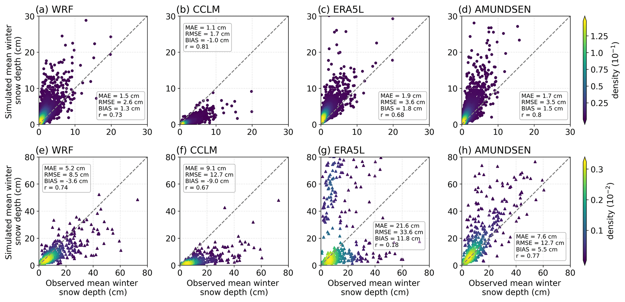
Figure 8Mean winter snow depth for each winter season and location in 1987–2018. The upper row (a–d) refers to locations with less than 5 cm mean winter snow depth (dots in Fig. 6), whereas the lower row shows locations above this threshold (triangles in Fig. 6).
3.3 Snow duration and cover
Mapping the number of snow days averaged for 1987–2018 leads to similar spatial patterns to the mean snow depth (compare Fig. 9 to Fig. 6), which also applies to the differences from the observations. CCLM generally underestimates the duration (Fig. 9b), whereas ERA5L generally overestimates it, apart from four locations in the northern low mountain ranges (Fig. 9c). WRF and AMUNDSEN show lower differences but a similar spatial pattern (Fig. 9a and d).
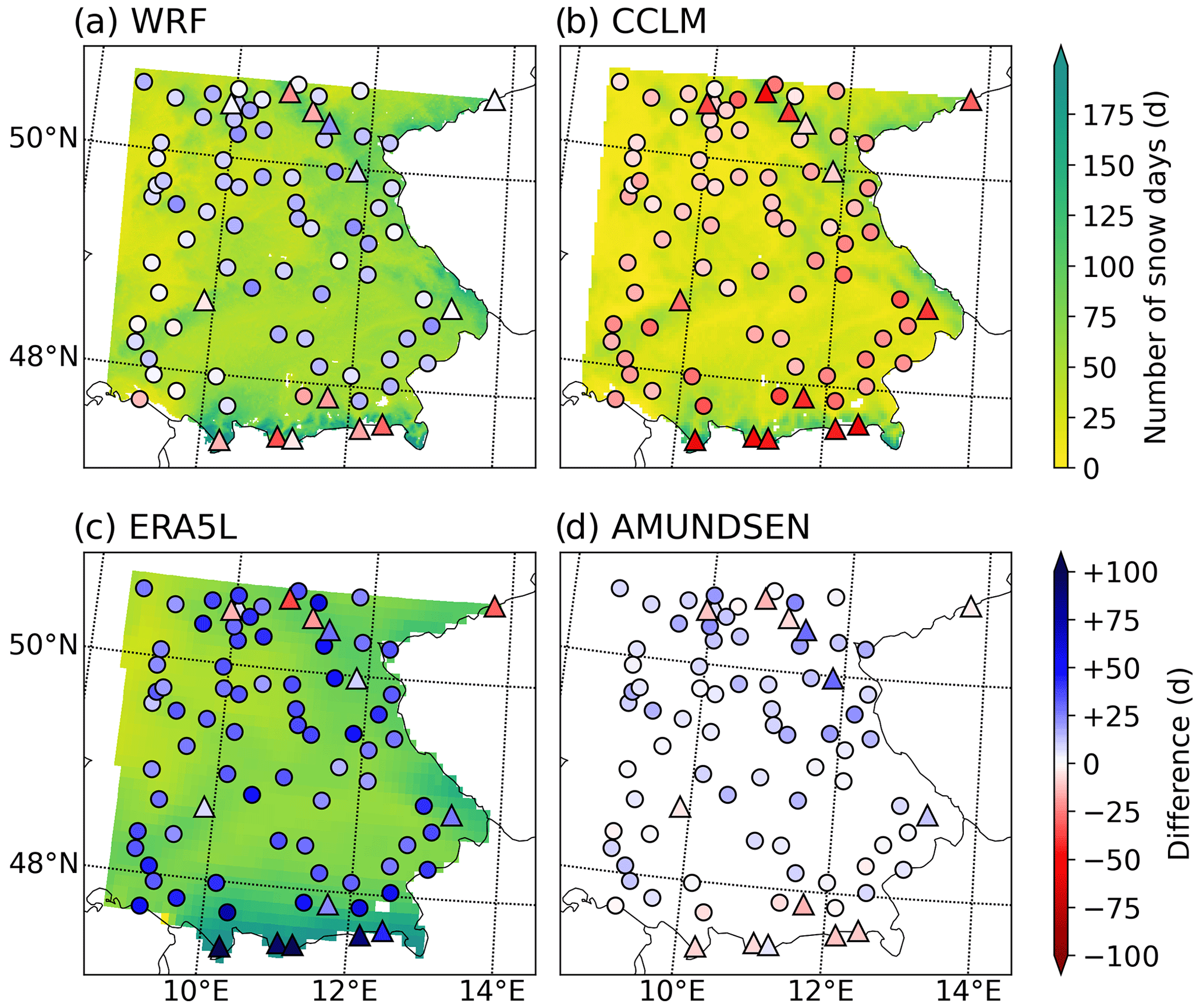
Figure 9Mean annual number of snow days during 1987–2018 simulated by the WRF model (a), CCLM (b), ERA5L (c), and AMUNDSEN (d). Snow days are defined as days with more than 1 cm snow depth. The differences at the stations (coloured dots) are calculated as model minus observation. A red (blue) colour refers to underestimation (overestimation) by the model.
A separate evaluation of each year is presented in Fig. 10, where WRF and AMUNDSEN show a strong rank correlation and comparably low error metrics. Despite high inter-seasonal and inter-station correlation, the CCLM simulation predicts, on average, 16 fewer snow days than observed at the low-lying localities (Fig. 10b) and 37 snow days fewer at snow-rich localities (Fig. 10f). ERA5L, on the other hand, simulates durations that are 29–35 d too long (Figs. 8c and g).
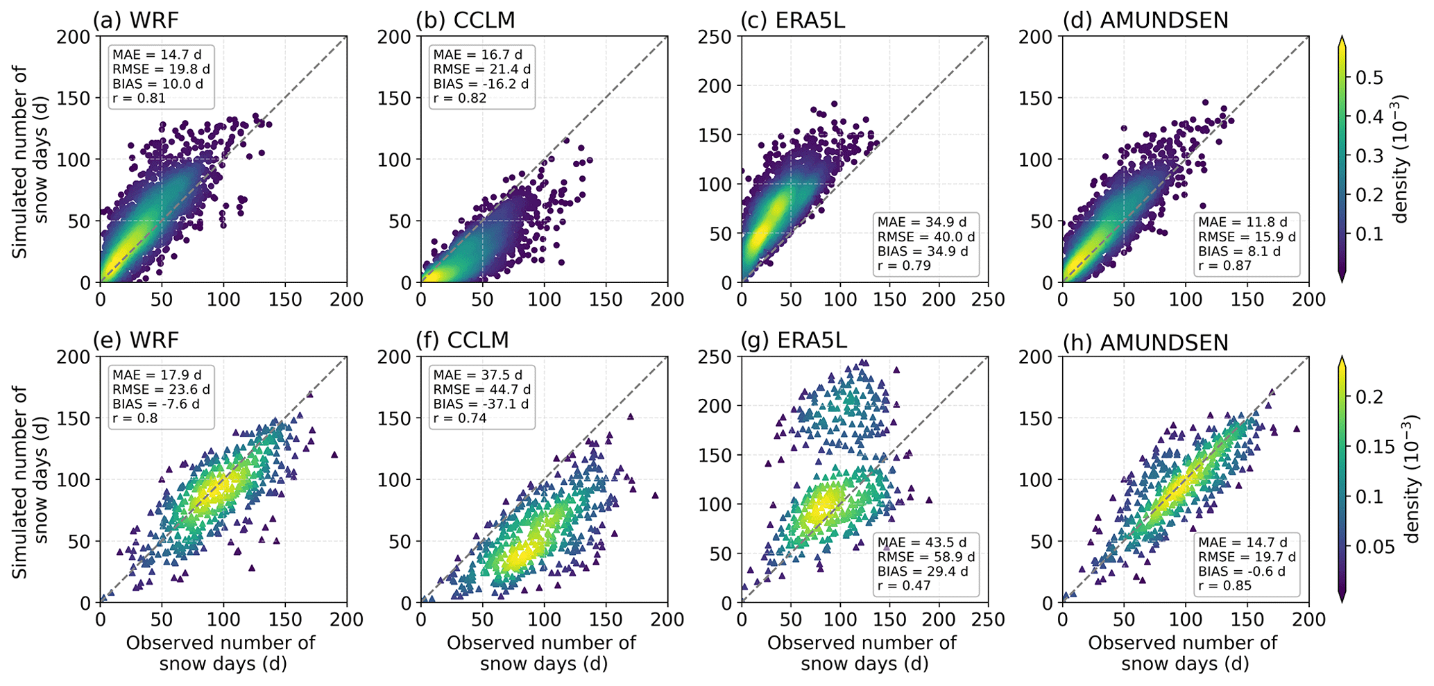
Figure 10Number of snow days for each year and location in 1987–2018. The upper row (a–d) refers to locations with less than 5 cm mean winter snow depth (dots in Fig. 9), whereas the lower row shows locations above this threshold (triangles in Fig. 9).
The snow cover fraction during December to February averaged for 2000–2018 amounts to 42 %, based on MODIS (see Fig. 11). The CCLM strongly underestimates the snow cover in the whole study area (20 %), resulting in less than half of the remotely sensed fraction. ERA5L shows overestimation in the southern Alpine part and slight underestimation in the remaining study area (Fig. 11c), amounting to 37 % over the whole study area. For the WRF simulation, this parameter is not openly available.
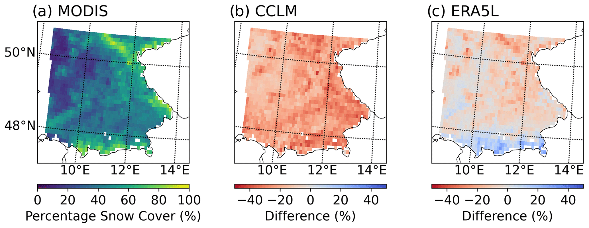
Figure 11Mean snow cover fraction during DJF averaged over the period 2000–2018. For the remote-sensing product (a, MODIS MOD10C1.061), only data with at least “okay” quality are considered. The differences (b, c) are calculated as model minus remote-sensing product, where a red (blue) colour refers to an underestimation (overestimation) of the model. The extended winter season (November to April) is shown in Fig. S2 in the Supplement.
3.4 White Christmas and short periods
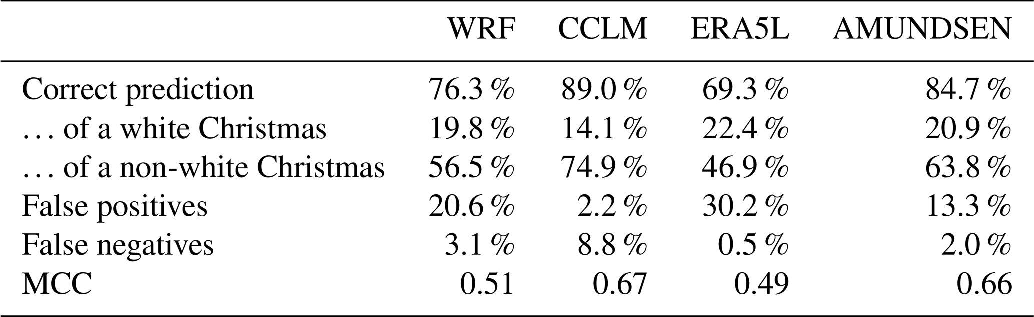
The tendencies to over- and underestimate the mean winter snow conditions (Sects. 3.2 and 3.3) also manifest when assessing shorter time periods than seasonal averages. There are four very different predictions for the percentage of white Christmases during 1987–2018. The spatial pattern follows the previous evaluations of mean snow depth and snow cover duration (compare Fig. S3 to Figs. 6 and 8). Averages over all seasons and locations are provided in Table 3. There, CCLM and AMUNDSEN are seen to outperform WRF and ERA5L, with Matthews correlation coefficients of 0.67 for CCLM and 0.66 for AMUNDSEN, but they also show a tendency to underestimate (CCLM) and overestimate (AMUNDSEN) the occurrence of a white Christmas.
Table 3White Christmas percentages averaged over 1987–2018 and all locations in the study area.
As a white Christmas refers to only one selected time window in the year, we furthermore assess all 3 d moving windows over the extended winter season. In this case, the MCC scores slightly improve (see MCC_3d in Table 4).
Table 4MCC scores for 3 d moving windows with at least 1 d where the snow depth is above 1 cm, averaged over 1987–2018 and all locations in the study area. MCC scores for 5 d moving windows with snow depths above 10 cm on all 5 d.
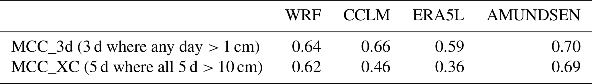
As a proxy for the opportunity to do cross-country skiing, we assess 5 d moving windows during which the snow depth needs to be above 10 cm on all 5 d. This analysis is only carried out at the locations where the mean snow depth is above 5 cm (see the triangular markers in Fig. 1). For these conditions, the MCC scores of CCLM and ERA5L drop, whereas the MCC scores of WRF and AMUNDSEN amount to 0.62 and 0.69, respectively (MCC_XC in Table 4).
3.5 Evaluation of extreme snow depths
Figure 12 provides simulated and observed maxima of snow depth, with the WRF model showing small deviations and almost no bias at low-lying localities (Fig. 12a). Observations at snow-rich locations are slightly underestimated (Fig. 12e). The general underestimation of CCLM also applies for the maximum snow depths (Fig. 12b and f). The strong negative bias suggests that the model is not appropriate to assess extreme snow depths, as already described in the documentation by Doms et al. (2021). The rank correlations (r) of 0.79 and 0.71, however, suggest that the model is able to reproduce inter-site and interannual differences well. ERA5L can even reproduce annual extreme snow depths at low-lying stations slightly better than WRF can (Fig. 12c), but it tends to overestimate extreme snow depths, yielding the highest RMSE and lowest rank correlation over complex terrain (Fig. 12g). The largest deviations occur for snow depths above 50 cm over complex topography (Fig. 12g). The difference in the mean annual maximum snow depth for the 83 stations correlates strongly with the elevation bias of ERA5L (see Fig. 4c and f and Table S1 in the Supplement; r=0.91). We argue that the overly low spatial resolution is a major contributor to the deviations of extreme snow dynamics in the low mountain ranges and Alps. For the other models, no significant correlation is found for this dependence. AMUNDSEN slightly overpredicts extreme snow depths, with a moderate positive bias seen for all stations.
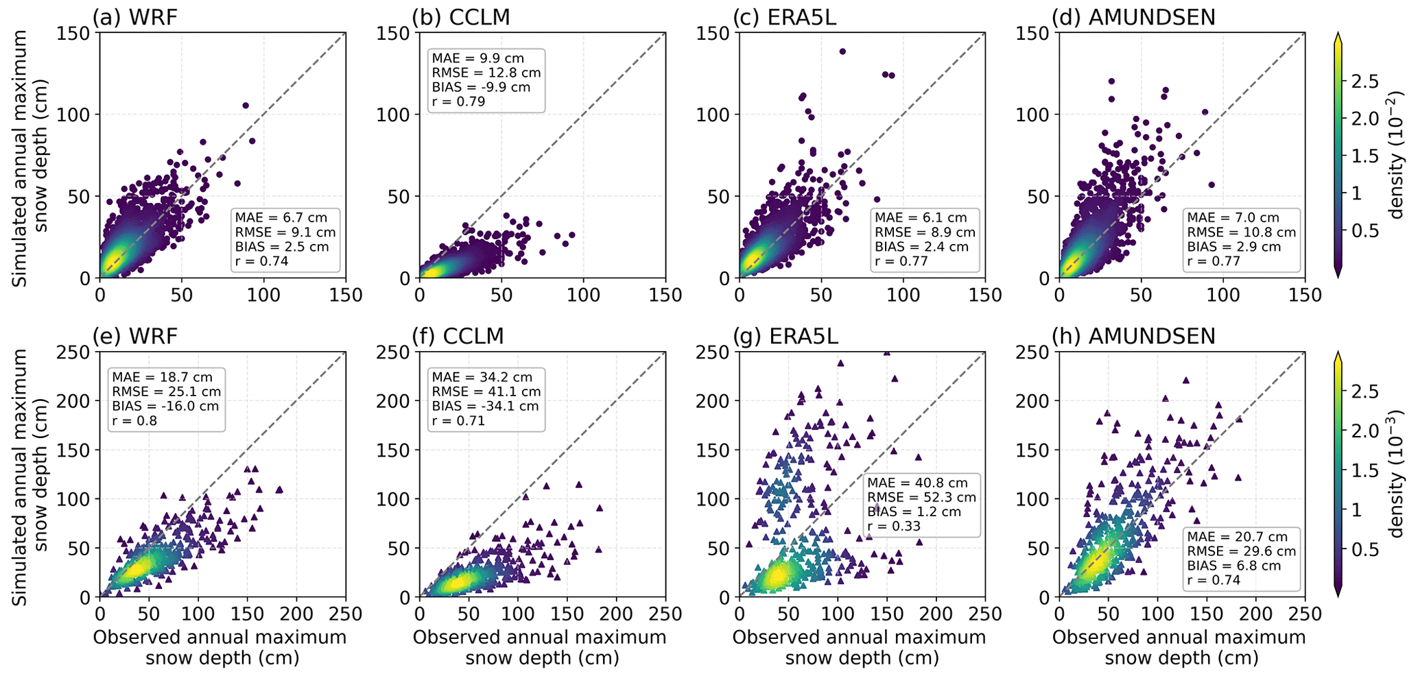
Figure 12Annual maxima of snow depth for each year and location in 1987–2018. The upper row (a–d) refers to locations with less than 5 cm mean winter snow depth, whereas the lower row shows locations above this threshold.
We further assess if the GEV location parameters μ fitted on the modelled annual maxima of snow depth are within the 95 % confidence interval of the respective observation-based μ for each station (see Fig. 13). We find that CCLM is not able to reproduce this extreme-value statistical property within the observational range at any station. AMUNDSEN shows the highest level of agreement (57 % of stations), followed by WRF (51 %) and ERA5L (34 %). ERA5L cannot capture the rank correlation between the stations (r=0.61) as well as the other models (r > 0.91) due to larger deviations at snow-rich localities. The WRF model shows good agreement for stations with location parameters below 20 mm but underestimates the upper range (Fig. 13).
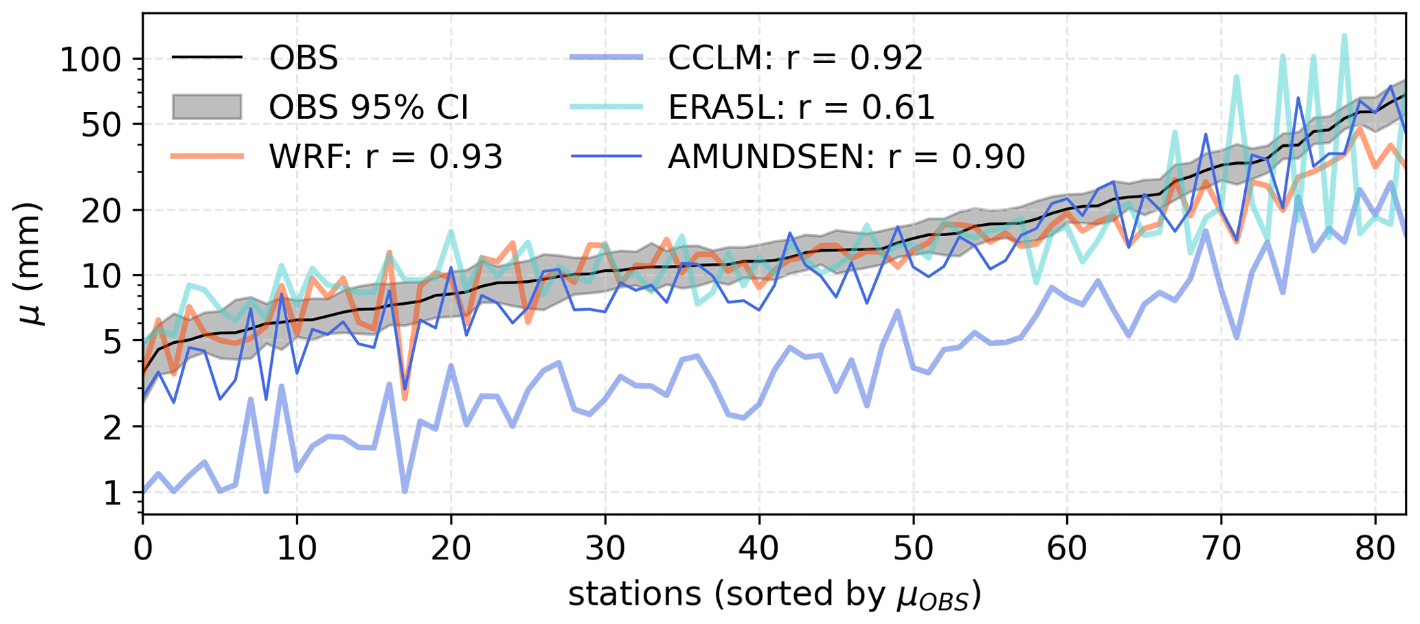
Figure 13Fitted GEV location parameters for the observed and simulated annual maxima of snow depth. Note the logarithmic scaling of the y axis.
The seasonality of the annual maximum snow depth is visualised as the bivariate kernel density estimation (Fig. 14). The general timing of annual maximum snow depths is reproduced well by all models (compare the marginal histograms in Fig. 14), although the CCLM does not simulate enough snow depth maxima after February (Fig. 14b). For the comparison of each station–year combination in 1987–2018, the WRF model (Fig. 14a) shows the highest agreement with low bias.
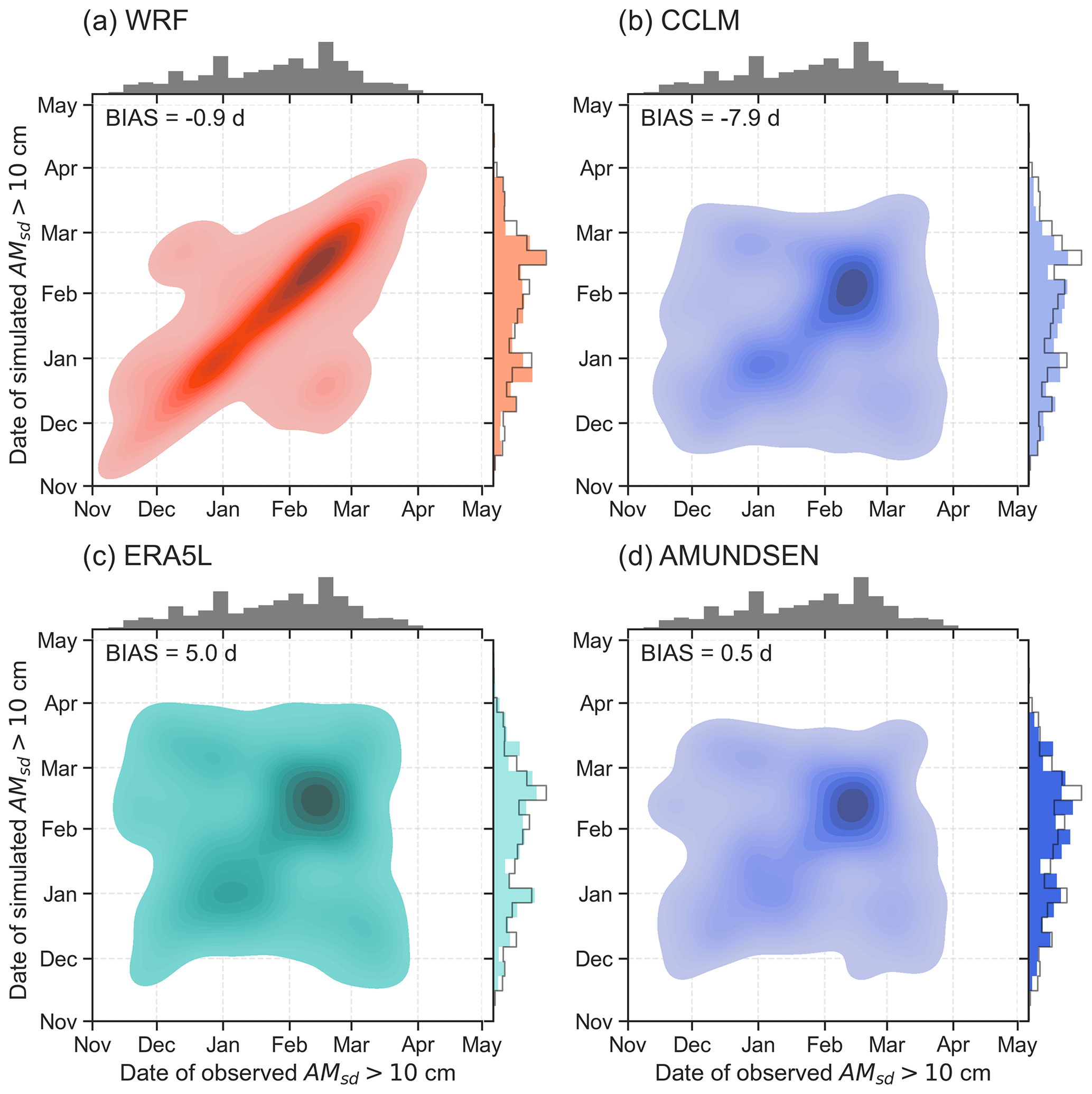
Figure 14Bivariate kernel density plot of dates for annual snow-depth maxima above 10 cm for each year and location in 1987–2018 simulated by the WRF model (a), CCLM (b), ERA5L (c), and AMUNDSEN (d). Marginal distributions aggregated over all years and stations are given as histograms at the edges of the plots. The solid grey histogram and grey line histogram refer to the observations.
The representation of snow dynamics is important for impact assessments (see Sect. 1) and for the coupling within the regional climate model in the WRF and CCLM.
Depending on the measure of interest, the evaluation yields very different results, even though all simulations are driven by the same large-scale atmospheric conditions from ERA5. This indicates the presence of large model uncertainties regarding snow dynamics. These uncertainties result from different sources and are interconnected, which is why they are difficult to disentangle (Monteiro and Morin, 2023).
In addition, the comparison between point in situ measurements and gridded simulations is affected by the spatial variability of snow depth (Clark et al., 2011). The standardised local environment of the climate station might not capture the land cover and topography of the surrounding area, which in turn governs the gridded simulation (Meromy et al., 2012). The resulting deviations are expected to be higher for a coarser model resolution, a complex topography, in areas covered by forest vegetation, and in open areas prone to wind redistribution (Mortimer et al., 2020).
Furthermore, the rather low station density leads to unsatisfactory coverage in parts of the study area. However, the stations were selected according to their low amounts of missing data, and they represent the range of elevations between 150 and 1000 m well (Fig. 2). Additionally, the analysis was supplemented by satellite data from MODIS to ensure spatial representativeness.
In Table 2, the significant correlation between elevation bias and the biases of temperature and precipitation for ERA5L indicates that the spatial resolution of the model contributes considerably to the deviations. Due to the 9 km grid cell size, the complexity of the terrain cannot be reproduced in parts of the study area.
For the WRF simulation, a significant correlation between elevation and temperature bias is found, indicating that the less-elevated stations show a more pronounced cold bias. Overall, the WRF shows a systematic underestimation of temperature. Collier and Mölg (2020) relate this behaviour to a miscalculation of the mean grid-cell albedo in NOAH_MP (Tomasi et al., 2017). Generally, it should be emphasised that the albedo of exposed snow surfaces differs from that of snow over surfaces with shrub or forest vegetation. The areal simulations of WRF, CCLM, and ERA5L represent mean grid-cell values and depend on the land cover parametrisation of the respective grid cell. At the point representing the climate station, exposed snow areas predominate due to the standardised environmental conditions with grass cover. Hence, the comparability is limited for grid cells in which the model assumes there to be forest. Furthermore, the temporal variability of snow and albedo at the point scale can be higher than for areal averages (Clark et al., 2011). Remote-sensing products provide observation-based areal estimations for the albedo. We compare the albedo of the WRF, CCLM, and ERA5L simulations to the remote-sensing product MODIS MCD43C3 at 0.05° resolution (Schaaf and Wang, 2021) for the whole study area without the Alps (Fig. 15a) and for the Alps only (Fig. 15b) and confirm the strong overestimation within the WRF simulation.
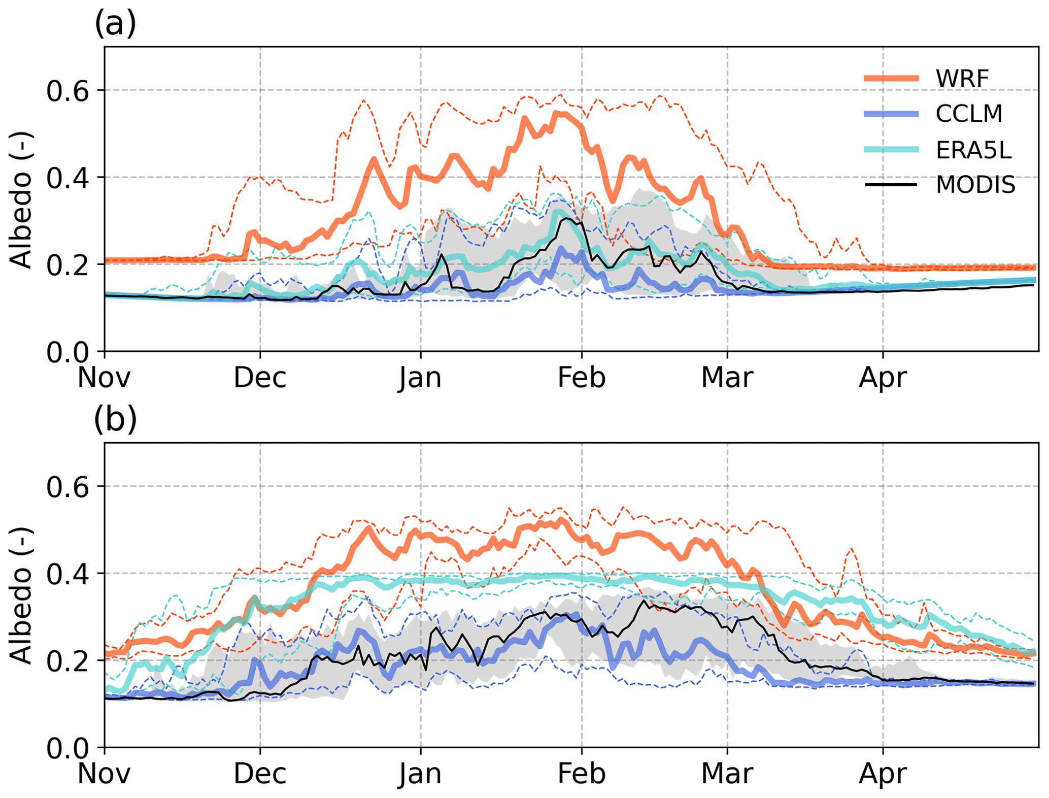
Figure 15Albedo for the years 2000 to 2018. Daily albedo values are averaged over the whole study area (a) without the Alps and (b) for the Alps (south of 47.8° N and west of 10° E) only. The thick lines denote the median over all seasons. The area between the dashed lines and the grey-shaded area shows the inner-50 % range. For the remote-sensing product (MODIS MCD43C3), only data of at least “mixed” or good quality are considered, and at least half of the area needs to be covered with valid values.
ERA5L agrees over the non-Alpine area but overestimates in the Alps, with the strongest deviations occurring during early and late winter, reflecting the huge positive bias in the snow cover duration in the Alps (Fig. 9c). As ERA5L is an offline simulation driven by the climate of ERA5, the simulated albedo of ERA5L has only very minor effects on the temperatures shown in Fig. 3. The empirical parametrisation in CCLM agrees with MODIS for the first month (until mid-January and the beginning of February, respectively), but it underestimates the albedo afterwards. This is due to the underestimation of snow cover duration (Figs. 9b and 10b and f). As the land surface scheme TERRA_ML is run coupled with the atmospheric simulation, the albedo affects the simulated air temperature. However, the low biases in temperature (Fig. 3) suggest that the overall representation of the albedo in TERRA_ML does not translate into strong discrepancies in temperature for CCLM.
The different albedo simulations are compared over one selected winter season at five locations (Fig. S4 and Table S2 in the Supplement). Here, the negative temperature bias of the WRF simulations (Fig. 3) occurs mainly during periods with snow and, therefore, overestimated snow albedo (Fig. 16), confirming the assumption by Collier and Mölg (2020). Liu et al. (2021) propose a modified snow-albedo scheme for the NOAH_MP with lower albedo values on average than the default scheme, improving the representation of sensible heat flux, air temperature, and snow depth over the Tibetan Plateau. The albedo scheme of AMUNDSEN for exposed snow surfaces yields a similar albedo estimation to the WRF simulation for non-forested grid cells (Fig. S4). However, AMUNDSEN represents the point scale and is not run coupled with atmospheric modelling, so it does not affect the modelled climate.
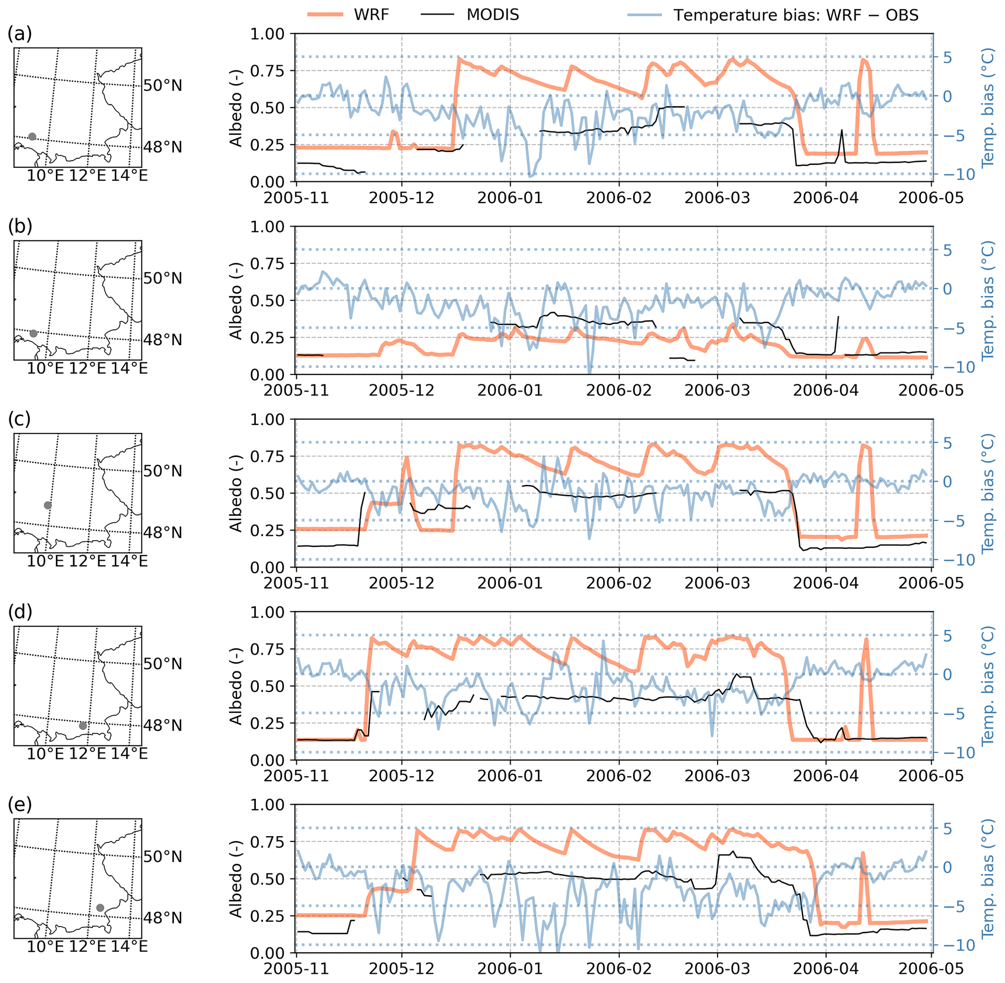
Figure 16Daily albedo based on remote sensing (MODIS MCD43C3) and the WRF simulation over the winter season 2005/06 at five locations. For the MODIS time series, only data of at least “mixed” or good quality are shown. The second y axis shows the temperature bias of WRF compared to the weather stations. The vegetation type of the respective WRF grid cell (which affects the simulated albedo) is grassland (a, c, e), evergreen needleleaf forest (b), and urban and built-up land (d).
Furthermore, the snow surface albedo also governs the energy budget of the snow layer (Essery et al., 2013). The slight overestimation of mean snow depth and snow cover duration in the WRF simulations can be attributed to the biases in albedo and temperature. Applying different albedo parametrisations induces considerable differences in the simulated snow depth and snow cover duration. For the WRF simulations, 17 of the 83 locations are classified as forest. The mean biases of winter snow depth and snow cover duration over all stations amount to +0.4 cm and +6.8 d (Figs. 8 and 10). For the 17 forest grid cells, however, the deviations amount to −0.9 cm and +3.2 d, whereas the remaining non-forested locations show larger overestimations of snow dynamics (+0.9 cm and +7.7 d).
Even though ERA5L simulates a lower surface albedo over non-forested areas than WRF, it shows the strongest positive bias in mean snow depth and snow cover duration. The largest overestimations are located in the (pre-)alpine areas in the south of the study area; however, the snow cover duration is overestimated for almost the whole region. Daloz et al. (2022) also report positive deviations of ERA5L in the extent, fraction, and duration of snow cover over Europe compared to MODIS. In an evaluation with various satellite-based data, Kouki et al. (2023) find that ERA5L also overestimates the SWE in the Northern Hemisphere in spring. Monteiro and Morin (2023) confirm these findings over the Alps, where ERA5L shows the strongest positive bias in snow depth and snow cover duration of all intercompared models for all elevation ranges. When developing the new snow scheme for the next-generation ECLand model (Boussetta et al., 2021), these deviations should be accounted for.
Despite its skilful reproduction of precipitation and air temperature (Fig. 3b and e) and realistic ranges of simulated albedo (Figs. 15 and S4), CCLM simulates snow depth, number of snow days, snow cover fraction, and snow depth extremes with large negative biases. In contrast to our analysis, Lüthi et al. (2019) diagnosed a slight overestimation of SWE over Switzerland for a similar model setup, i.e. employing COSMO-CLM at 2.2 km with the TERRA_ML land-surface model driven by ERA-Interim (Ban et al., 2014). The CCLM and TERRA_ML setup analysed in this study, however, suggests that it is not appropriate for any further impact analysis.
Based on the same climatic conditions as in CCLM, AMUNDSEN tends to slightly overpredict snow depth and snow cover duration. The larger overestimations of the AMUNDSEN simulation are located in the low mountain ranges (Figs. 6d and 9d). Especially during snowy winter seasons, AMUNDSEN produces snow depths that are heavily overestimated. An exploration of these locations reveals that the CCLM has a general positive precipitation bias there, which is partly diagnosed by the rank correlation of r=0.32 between elevation and precipitation bias. However, this positive bias mostly applies to the stations above 500 m elevation north of 48.5° N (Fig. S5 in the Supplement).
Apart from the sources of uncertainties discussed above, the parametrisation of snow density also adds uncertainty (Essery et al., 2013). The density of newly fallen snow is usually in the range of 20 to 300 kg m−3 and depends on whether the air temperature induces dry to wet snow characteristics and on the wind speed (Lee et al., 2023). Here, all models parametrise the density of fresh snow differently depending on the temperature, with only ERA5L additionally including the near-surface wind speed. Also, compaction and metamorphism are parametrised differently, with three models (WRF, ERA5L, AMUNDSEN) following Anderson (1976) for the description of compaction. This semi-empirical scheme is widely used in snow and land-surface models and assumes a two-stage compaction due to metamorphism and pressure from the snow mass above (Aschauer et al., 2023). It further employs a viscosity coefficient that is dependent on temperature to model stress-induced compaction. Settling of the snowpack is described with wet snow in the respective snow layer. Even though this approach is quite sophisticated, not all processes leading to densification are captured, which may partly contribute to deviations between the modelled and observed snow depth. Koch et al. (2019) note that rain-on-snow events or periods of warm weather, which are expected to occur in the elevation range of our study area, may cause such deviations. Hence, the estimation of snow density contributes to inter-model differences and also induces uncertainty in the evaluation of snow depth. However, neither snow density nor SWE is measured at the climate stations, so they cannot be evaluated.
In addition, the number of snow layers considered is found to be relevant to the reproduction of snow depth and cover (Arduini et al., 2019; Jin et al., 1999). Jin et al. (1999) emphasise that using multiple snow layers improves the representation of temporal variability at diurnal and seasonal timescales. Xue et al. (2003) highlight the importance of multiple snow layers for the ablation period, as using multiple layers allows the separation of the soil temperature from the surface temperature. This is considered beneficial for reproducing the variability of snow surface temperatures, as single-layer setups tend to simulate surface temperatures that are around freezing point, with little variability. Here, the multi-layer setups of WRF and AMUNDSEN show better performance for the snow cover duration and the timing and intensity of annual maximum daily snow. The new five-layer snow scheme of ECLand (Arduini et al., 2019) improves the simulation of melting periods compared to the single-layer scheme of ERA5L.
The evaluation of simulations of short periods within the year is very relevant to tourism-related topics. AMUNDSEN can achieve the highest classification scores for the prediction of a white Christmas, snow during any 3 d period, and snow consistently above 10 cm depth during a 5 d period. All models perform with MCCs in the range from 0.36 to 0.70, indicating a moderate-to-strong positive relationship between the model classification and the observation. Still, the tendency to classify a period as “snowy” follows the general behaviour of the respective model to overestimate or underestimate snow depth.
For the representation of extremes in snow depth, the differences between point scale and areal simulations may affect the comparison. Averaged over all locations, one would expect a slight underestimation of simulated annual maximum snow depth, as the climate station shows an exposed snow surface, whereas grid cells may represent mixed surfaces or forested areas. Furthermore, the point scale shows a higher temporal variability than areal averages, leading to more pronounced extremes. Still, even considering these limitations, the assessment reveals that WRF, AMUNDSEN, and ERA5L can reproduce snow depth extremes well in low-lying areas, whereas WRF and AMUNDSEN can clearly add value to the representation of extremes over complex terrain compared to ERA5L.
In conclusion, the high-resolution climate model WRF and the hydro-climatological model AMUNDSEN driven by CCLM can add value compared to the state-of-the-art reanalysis product ERA5L. CCLM provides a skilful reproduction of the climate but systematically underestimates all snow dynamics. Based on this assessment, one can draw some recommendations for model application and further model development.
First, simulations of snow dynamics have to be carefully evaluated according to the intended use of the data. As also shown by other studies, such as SnowMIP (Essery et al., 2013), this evaluation has confirmed that the setup of the regional climate model or land-surface model can greatly influence the snow depth simulations, even when they are all driven by the same large-scale atmospheric conditions. Here, we have shown that this variability also occurs at lower elevation ranges (150 to 1000 m). With coarse-resolution climate models, the complexity of the terrain often prevents comparability between the results of the climate model and the observations. The 83 locations in southern Germany show different degrees of terrain complexity, but the resolution of the high-resolution RCMs is sufficient to reproduce the elevations with moderate-to-low deviations. For the representation of the winter climate, high-resolution RCMs can add value compared to ERA5L. This also translates into a benefit for the representation of snow dynamics, except if the snow model is not appropriately parametrised for the study area (as in the case of CCLM and TERRA_ML). Hence, for a study area with topography of medium complexity, we can generally recommend the use of the snow depth from a high-resolution RCM snow scheme. In case of a well-represented climate but strong biases in the snow simulation (as in the CCLM here), the added value of the high-resolution climate simulation can be utilised by setting up a separate snow model (such as AMUNDSEN in this study), where a calibration to the local conditions might further improve the reproduction of observed snow depth. Hence, for local and regional snow impact assessments, high-resolution climate models can be a valuable tool. However, we recommend that climate and snow biases should be analysed carefully. In order to fully make use of this potential in high-resolution simulations, it would be advisable to store and provide not only the simulated snow depth but also the SWE and fraction of snow cover.
Second, with regard to future climate model and land-surface model development, the evaluation in this study has revealed some potential for improvement. A thorough review or revision of the TERRA_ML snow scheme in the ICON-CLM model is recommended. For NOAH_MP, the problem of overly high albedos has been addressed by Tomasi et al. (2017), and the resulting cold bias during winter as well as the overestimation of snow dynamics were confirmed for southern Germany in this study. New albedo parametrisations are already proposed (Liu et al., 2021) and will be evaluated. The overprediction of mean snow depth and snow cover duration in the ERA5L simulations partly result from the elevation bias and the corresponding temperature bias. However, the general tendency to overestimate snow cover duration and the underestimation of extreme daily snow melting indicate that the snow scheme needs to be revised accordingly in the course of the development of the new ECLand model.
Generally, parametrisations and snow models for alpine and arctic areas tend to be developed and evaluated disproportionately infrequently (e.g. Essery et al., 2013; Krinner et al., 2018; Liu et al., 2021). This is understandable, as snow dynamics have a high relevance in these areas, and long records without non-natural influences are available. However, considering the relevance of snow-related impacts, it is also important to ensure that the snow dynamics in more densely populated areas are well represented in the simulations. Hence, we propose the study area in southern Germany as a testbed for further investigations, such as LUCAS phase 3 (Daloz et al., 2022).
On the other hand, high-resolution climate model or earth system model simulations could further improve our knowledge of snow dynamics in topographically highly complex regions, where state-of-the-art reanalysis data and earth system models show large deviations from observations (Daloz et al., 2020; Kouki et al., 2022). However, observations are sparsely distributed in these regions. Snowfall and snow storage play an important role in freshwater availability, with strong implications of rising temperatures (Simpkins, 2018). Hence, high-resolution models could support decision-making regarding water infrastructure design and management.
Lastly, we recommend evaluating the performance of snow models regarding extreme snow dynamics. Possible measures are proposed in this study, such as daily maxima of snow depth and their seasonality. They could be extended by assessing the daily maxima of snow melt and accumulation by analysing the SWE. Our knowledge about future snow dynamics depends on model simulations. Due to the high impacts of extreme snow conditions on human society, it is important to capture these events in the simulations.
The ERA5-Land data are available from https://doi.org/10.24381/cds.e2161bac (Muñoz-Sabater, 2019; Muñoz-Sabater et al., 2021), while the WRF simulations are stored at https://doi.org/10.17605/OSF.IO/AQ58B (Collier, 2020). The COSMO-CLM simulations are available from https://doi.org/10.5676/DWD/HOKLISIM_V2022.01 (Brienen et al., 2022). The observational data are provided by the German Weather Service at https://opendata.dwd.de/climate_environment/CDC/observations_germany/climate/daily/kl/historical/ (DWD, 2023). The MODIS snow cover fraction is available from https://doi.org/10.5067/MODIS/MOD10C1.061 (Hall and Riggs, 2021) and MODIS albedo data are available from https://doi.org/10.5067/MODIS/MCD43C3.061 (Schaaf and Wang, 2021).
The supplement related to this article is available online at: https://doi.org/10.5194/tc-18-1959-2024-supplement.
BP conceptualised the study, performed the simulations, and conducted the formal analysis. ASD contributed to the conceptualisation. BP prepared the original draft with significant contributions from ASD.
The contact author has declared that none of the authors has any competing interests.
Publisher's note: Copernicus Publications remains neutral with regard to jurisdictional claims made in the text, published maps, institutional affiliations, or any other geographical representation in this paper. While Copernicus Publications makes every effort to include appropriate place names, the final responsibility lies with the authors.
We cordially thank all of the following data provisioners (who or which are cited in the main article): Brienen et al. (2022), Collier (2020), the German Weather Service, and Muñoz-Sabater et al. (2021). The open-source version of AMUNDSEN written in Python (Warscher et al., 2021; https://github.com/openamundsen/openamundsen, last access: 20 June 2023) is cordially acknowledged. Further, we thank Susanne Brienen from the German Weather Service for information on the COSMO simulations and the provision of the albedo data. This research has been funded by the Deutsche Forschungsgemeinschaft (DFG, German Research Foundation) under Germany's Excellence Strategy – EXC 2037 “CLICCS – Climate, Climatic Change, and Society” – project no. 390683824, a contribution to the Center for Earth System Research and Sustainability (CEN) of Universität Hamburg.
This research has been supported by the Deutsche Forschungsgemeinschaft (grant no. EXC 2037, project no. 390683824).
This paper was edited by Michiel van den Broeke and reviewed by two anonymous referees.
Anderson, E. A.: A point energy and mass balance model of a snow cover, Tech. Rep. NWQ 19, NOAA, Office of Hydrology, National Weather Service, Silver Spring, MD, USA, https://repository.library.noaa.gov/view/noaa/6392 (last access: 19 July 2023), 1976.
ARD: Winterchaos in Bayern Tausende Stromausfälle – Retter im Dauereinsatz, https://www.tagesschau.de/inland/innenpolitik/bayern-winterchaos-stromausfaelle-100.html (last access: 27 February 2024), 2023.
Arduini, G., Balsamo, G., Dutra, E., Day, J. J., Sandu, I., Boussetta, S., and Haiden, T.: Impact of a Multi-Layer Snow Scheme on Near-Surface Weather Forecasts, J. Adv. Model. Earth Sy., 11, 4687–4710, https://doi.org/10.1029/2019MS001725, 2019.
Aschauer, J., Michel, A., Jonas, T., and Marty, C.: An empirical model to calculate snow depth from daily snow water equivalent: SWE2HS 1.0, Geosci. Model Dev., 16, 4063–4081, https://doi.org/10.5194/gmd-16-4063-2023, 2023.
Ban, N., Schmidli, J., and Schär, C.: Evaluation of the convection-resolving regional climate modeling approach in decade-long simulations, J. Geophys. Res.-Atmos., 119, 7889–7907, https://doi.org/10.1002/2014JD021478, 2014.
Barnett, T. P., Adam, J. C., and Lettenmaier, D. P.: Potential impacts of a warming climate on water availability in snow-dominated regions, Nature, 438, 303–309, https://doi.org/10.1038/nature04141, 2005.
Bausch, T. and Unseld, C.: Winter tourism in Germany is much more than skiing! consumer motives and implications to Alpine destination marketing, J. Vacat. Mark., 24, 203–217, https://doi.org/10.1177/1356766717691806, 2018.
Bednorz, E.: Heavy snow in Polish–German lowlands: large-scale synoptic reasons and economic impacts, Weather and Climate Extremes, 2, 1–6, https://doi.org/10.1016/j.wace.2013.10.007, 2013.
Berghuijs, W. R., Harrigan, S., Molnar, P., Slater, L. J., and Kirchner, J. W.: The relative importance of different flood-generating mechanisms across Europe, Water Resour. Res., 55, 4582–4593, https://doi.org/10.1029/2019WR024841, 2019.
Blume-Werry, G., Kreyling, J., Laudon, H., and Milbau, A.: Short-term climate change manipulation effects do not scale up to long-term legacies: effects of an absent snow cover on boreal forest plants, J. Ecol., 104, 1638–1648, https://doi.org/10.1111/1365-2745.12636, 2016.
Bocharov, G.: pyextremes – Extreme Value Analysis (EVA) in Python, https://georgebv.github.io/pyextremes/ (last access: 19 July 2023), 2022.
Boussetta, S., Balsamo, G., Arduini, G., Dutra, E., McNorton, J., Choulga, M., Agustí-Panareda, A., Beljaars, A., Wedi, N., Muñoz Sabater, J., de Rosnay, P., Sandu, I., Hadade, I., Carver, G., Mazzetti, C., Prudhomme, C., Yamazaki, D., and Zsoter, E.: ECLand: The ECMWF Land Surface Modelling System, Atmosphere, 12, 723, https://doi.org/10.3390/atmos12060723, 2021.
Braun, L. N.: Simulation of snowmelt-runoff in lowland and lower alpine regions of Switzerland, PhD thesis, ETH Zurich, https://doi.org/10.3929/ethz-a-000334295, 1984.
Brienen, S., Haller, M., Brauch, J., and Früh, B.: HoKliSim-De COSMO-CLM climate model simulation data version V2022.01, DWD [data set], https://doi.org/10.5676/DWD/HOKLISIM_V2022.01, 2022.
Chen, J., Li, C., Brissette, F. P., Chen, H., Wang, M., and Essou, G. R. C.: Impacts of correcting the inter-variable correlation of climate model outputs on hydrological modeling, J. Hydrol., 560, 326–341, https://doi.org/10.1016/j.jhydrol.2018.03.040, 2018.
Clark, M. P., Hendrikx, J., Slater, A. G., Kavetski, D., Anderson, B., Cullen, N. J., Kerr, T., Hreinsson, E. O., and Woods, R. A.: Representing spatial variability of snow water equivalent in hydrologic and land-surface models: A review, Water Resour. Res., 47, W07539, https://doi.org/10.1029/2011wr010745, 2011.
Coles, S.: An introduction to statistical modeling of extreme values, Springer, London, UK, https://doi.org/10.1007/978-1-4471-3675-0, 2001.
Collier, E.: BAYWRF, OSFHOME [data set], https://doi.org/10.17605/OSF.IO/AQ58B, 2020.
Collier, E. and Mölg, T.: BAYWRF: a high-resolution present-day climatological atmospheric dataset for Bavaria, Earth Syst. Sci. Data, 12, 3097–3112, https://doi.org/10.5194/essd-12-3097-2020, 2020.
Coppola, E., Sobolowski, S., Pichelli, E., Raffaele, F., Ahrens, B., Anders, I., Ban, N., Bastin, S., Belda, M., Belusic, D., Caldas-Alvarez, A., Cardoso, R. M., Davolio, S., Dobler, A., Fernandez, J., Fita, L., Fumiere, Q., Giorgi, F., Goergen, K., Güttler, I., Halenka, T., Heinzeller, D., Hodnebrog, Q., Jacob, D., Kartsios, S., Katragkou, E., Kendon, E., Khodayar, S., Kunstmann, H., Knist, S., Lavín-Gullón, A., Lind, P., Lorenz, T., Maraun, D., Marelle, L., van Meijgaard, E., Milovac, J., Myhre, G., Panitz, H. J., Piazza, M., Raffa, M., Raub, T., Rockel, B., Schär, C., Sieck, K., Soares, P. M. M., Somot, S., Srnec, L., Stocchi, P., Tölle, M. H., Truhetz, H., Vautard, R., de Vries, H., and Warrach-Sagi, K.: A first-of-its-kind multi-model convection permitting ensemble for investigating convective phenomena over Europe and the Mediterranean, Clim. Dynam., 43, 3–34, https://doi.org/10.1007/s00382-018-4521-8, 2020.
Croce, P., Formichi, P., Landi, F., Mercogliano, P., Bucchignani, E., Dosio, A., and Dimova, S.: The snow load in Europe and the climate change, Climate Risk Management, 20, 138–154, https://doi.org/10.1016/j.crm.2018.03.001, 2018.
Daloz, A. S., Mateling, M., L'Ecuyer, T., Kulie, M., Wood, N. B., Durand, M., Wrzesien, M., Stjern, C. W., and Dimri, A. P.: How much snow falls in the world's mountains? A first look at mountain snowfall estimates in A-train observations and reanalyses, The Cryosphere, 14, 3195–3207, https://doi.org/10.5194/tc-14-3195-2020, 2020.
Daloz, A. S., Schwingshackl, C., Mooney, P., Strada, S., Rechid, D., Davin, E. L., Katragkou, E., de Noblet-Ducoudré, N., Belda, M., Halenka, T., Breil, M., Cardoso, R. M., Hoffmann, P., Lima, D. C. A., Meier, R., Soares, P. M. M., Sofiadis, G., Strandberg, G., Toelle, M. H., and Lund, M. T.: Land–atmosphere interactions in sub-polar and alpine climates in the CORDEX flagship pilot study Land Use and Climate Across Scales (LUCAS) models – Part 1: Evaluation of the snow-albedo effect, The Cryosphere, 16, 2403–2419, https://doi.org/10.5194/tc-16-2403-2022, 2022.
Daudt, R. C., Wulf, H., Hafner, E. D., Bühler, Y., Schindler, K., and Wegner, J. D.: Snow depth estimation at country-scale with high spatial and temporal resolution, ISPRS J. Photogramm., 197, 105–121, https://doi.org/10.1016/j.isprsjprs.2023.01.017, 2023.
DIN: DIN 1055-5, 2005-07, Einwirkungen auf Tragwerke – Teil 5: Schnee- und Eislasten, Deutsches Institut für Normung e.V., Beuth-Verlag, 24 pp., 2005.
Doll, C., Trinks, C., Sedlacek, N., Pelikan, V., Comes, T., and Schultmann, F.: Adapting rail and road networks to weather extremes: case studies for southern Germany and Austria, Nat. Hazards, 72, 63–85, https://doi.org/10.1007/s11069-013-0969-3, 2014.
Doms, G., Förstner, J., Heise, E., Herzog, H. J., Mironov, D., Raschendorfer, M., Reinhardt, T., Ritter, B., Schrodin, R., Schulz, J.-P., and Vofel, G.: A Description of the Nonhydrostatic Regional COSMO-Model – Part II: Physical Parameterizations, Deutscher Wetterdienst DWD, Offenbach, 2021.
Dong C. and Menzel, L.: Recent snow cover changes over central European low mountain ranges, Hydrol. Process., 34, 321–338, https://doi.org/10.1002/hyp.13586, 2020.
Durre, I. and Squires, M. F.: White Christmas? An Application of NOAA's 1981–2010 Daily Normals, B. Am. Meteorol. Soc., 96, 1853–1858, https://doi.org/10.1175/BAMS-D-15-00038.1, 2015.
Dutra, E., Balsamo, G., Viterbo, P., Miranda, P. M., Beljaars, A., Schär, C., and Elder, K.: An improved snow scheme for the ECMWF land surface model: description and offline validation, J. Hydrometeorol., 11, 899–916, https://doi.org/10.1175/2010JHM1249.1, 2010.
DWD (German Weather Service): Weiße Weihnachten – eine Frage des Standortes, https://www.dwd.de/DE/wetter/thema_des_tages/2020/12/24.html (last access: 19 July 2023), 2020.
DWD (German Weather Service): Daily climate data, DWD [data set], https://opendata.dwd.de/climate_environment/CDC/observations_germany/climate/daily/kl/historical/, last access: 13 June 2023.
ECMWF (Ed.): IFS documentation Cy45r1 Operational implementation 5 June 2018 PART IV: physical processes, Shinfield Park, Reading, England, UK, 223, https://doi.org/10.21957/4whwo8jw0, 2018.
Essery, R., Morin, S., Lejeune, Y., and Ménard, C.: A comparison of 1701 snow models using observations from an alpine site, Adv. Water Resour., 55, 131–148, https://doi.org/10.1016/j.advwatres.2012.07.013, 2013.
Foreman-Mackey, D., Hogg, D. W., Lang, D., and Goodman, J.: emcee: The MCMC Hammer, Publ. Astron. Soc. Pac., 125, 306–312, https://doi.org/10.1086/670067, 2013.
Frei, P., Kotlarski, S., Liniger, M. A., and Schär, C.: Future snowfall in the Alps: projections based on the EURO-CORDEX regional climate models, The Cryosphere, 12, 1–24, https://doi.org/10.5194/tc-12-1-2018, 2018.
Frese, M. and Blaß, H. J.: Statistics of damages to timber structures in Germany, Eng. Struct., 33, 2969–2977, https://doi.org/10.1016/j.engstruct.2011.02.030, 2011.
Gavazov, K., Ingrisch, J., Hasibeder, R., Mills, R. T. E., Buttler, A., Gleixner, G., Pumpanen, J., and Bahn, M.: Winter ecology of a subalpine grassland: effects of snow removal on soil respiration, microbial structure and function, Sci. Total Environ., 590–591, 316–324, https://doi.org/10.1016/j.scitotenv.2017.03.010, 2017.
Gerhold, L., Wahl, S., and Dombrowsky, W. R.: Risk perception and emergency food preparedness in Germany, Int. J. Disast. Risk Re., 37, 101183, https://doi.org/10.1016/j.ijdrr.2019.101183, 2019.
Girons Lopez, M., Vis, M. J. P., Jenicek, M., Griessinger, N., and Seibert, J.: Assessing the degree of detail of temperature-based snow routines for runoff modelling in mountainous areas in central Europe, Hydrol. Earth Syst. Sci., 24, 4441–4461, https://doi.org/10.5194/hess-24-4441-2020, 2020.
Hagen, P. and Mese, O.: Schneefälle: Wer zahlt für die Schäden?, https://www.sueddeutsche.de/wirtschaft/schneechaos-deutschland-versicherung-schaeden-zahlen-1.6314022 (last access: 27 February 2024), 2023.
Hall, D. K. and Riggs, G. A.: MODIS/Terra Snow Cover Daily L3 Global 0.05Deg CMG, Version 61, NASA NSIDC DAAC, Boulder, Colorado, USA [data set], https://doi.org/10.5067/MODIS/MOD10C1.061, 2021.
Hammer, H. L.: Statistical models for short- and long-term forecasts of snow depth, J. Appl. Stat., 45, 1133–1156, https://doi.org/10.1080/02664763.2017.1357683, 2018.
Hanzer, F., Helfricht, K., Marke, T., and Strasser, U.: Multilevel spatiotemporal validation of snow/ice mass balance and runoff modeling in glacierized catchments, The Cryosphere, 10, 1859–1881, https://doi.org/10.5194/tc-10-1859-2016, 2016.
Hanzer, F., Förster, K., Nemec, J., and Strasser, U.: Projected cryospheric and hydrological impacts of 21st century climate change in the Ötztal Alps (Austria) simulated using a physically based approach, Hydrol. Earth Syst. Sci., 22, 1593–1614, https://doi.org/10.5194/hess-22-1593-2018, 2018.
Harley, T. A.: Nice weather for the time of year: the British obsession with the weather, in: Weather, climate, culture, edited by: Strauss, S. and Orlove, B., Routledge, 103–120, https://doi.org/10.4324/9781003103264, 2003.
Hersbach, H., Bell, B., Berrisford, P., Hirahara, S., Horányi, A., Muñoz-Sabater, J., Nicolas, J., Peubey, C., Radu, R., Schepers, D., Simmons, A., Soci, C., Abdalla, S., Abellan, X., Balsamo, G., Bechtold, P., Biavati, G., Bidlot, J., Bonavita, M., Chiara, G. D., Dahlgren, P., Dee, D., Diamantakis, M., Dragani, R., Flemming, J., Forbes, R., Fuentes, M., Geer, A., Haimberger, L., Healy, S., Hogan, R. J., Hólm, E., Janisková, M., Keeley, S., Laloyaux, P., Lopez, P., Lupu, C., Radnoti, G., Rosnay, P. de, Rozum, I., Vamborg, F., Villaume, S., and Thépaut, J.-N.: The ERA5 global reanalysis, Q. J. Roy. Meteor. Soc., 146, 1999–2049, https://doi.org/10.1002/qj.3803, 2020.
HND (Hochwassernachrichtendienst Bayern): Station München Stadt, https://www.hnd.bayern.de/schnee/donau_bis_kelheim/muenchen-stadt-10865?addhr=false&begin=25.11.2023&end=12.12.2023, last access: 27 February 2024.
Hodeck, A. and Hovemann, G.: Destination Choice In German Winter Sport Tourism: Empirical Findings, Pol. J. Sport Tour., 22, 114–117, https://doi.org/10.1515/pjst-2015-0019, 2015.
Jin, J., Gao, X., Yang, Z.-L., Bales, R. C., Sorooshian, S., Dickinson, R. E., Sun, S. F., and Wu, G. X.: Comparative Analyses of Physically Based Snowmelt Models for Climate Simulations, J. Climate, 12, 2643–2657, https://doi.org/10.1175/1520-0442(1999)012<2643:CAOPBS>2.0.CO;2, 1999.
Jordan, R.: A one-dimensional temperature model for a snow cover: Technical documentation for SNTHERM 89, Tech. rep., Hanover, NH, https://hdl.handle.net/11681/11677 (last access: 19 July 2023), 1991.
Koch, F., Henkel, P., Appel, F., Schmid, L., Bach, H., Lamm, M., Prasch, M., Schweizer, J., and Mauser, W.: Retrieval of Snow Water Equivalent, Liquid Water Content, and Snow Height of Dry and Wet Snow by Combining GPS Signal Attenuation and Time Delay, Water Resour. Res., 55, 4465–4487, https://doi.org/10.1029/2018WR024431, 2019.
Kouki, K., Räisänen, P., Luojus, K., Luomaranta, A., and Riihelä, A.: Evaluation of Northern Hemisphere snow water equivalent in CMIP6 models during 1982–2014, The Cryosphere, 16, 1007–1030, https://doi.org/10.5194/tc-16-1007-2022, 2022.
Kouki, K., Luojus, K., and Riihelä, A.: Evaluation of snow cover properties in ERA5 and ERA5-Land with several satellite-based datasets in the Northern Hemisphere in spring 1982–2018, The Cryosphere, 17, 5007–5026, https://doi.org/10.5194/tc-17-5007-2023, 2023.
Krinner, G., Derksen, C., Essery, R., Flanner, M., Hagemann, S., Clark, M., Hall, A., Rott, H., Brutel-Vuilmet, C., Kim, H., Ménard, C. B., Mudryk, L., Thackeray, C., Wang, L., Arduini, G., Balsamo, G., Bartlett, P., Boike, J., Boone, A., Chéruy, F., Colin, J., Cuntz, M., Dai, Y., Decharme, B., Derry, J., Ducharne, A., Dutra, E., Fang, X., Fierz, C., Ghattas, J., Gusev, Y., Haverd, V., Kontu, A., Lafaysse, M., Law, R., Lawrence, D., Li, W., Marke, T., Marks, D., Ménégoz, M., Nasonova, O., Nitta, T., Niwano, M., Pomeroy, J., Raleigh, M. S., Schaedler, G., Semenov, V., Smirnova, T. G., Stacke, T., Strasser, U., Svenson, S., Turkov, D., Wang, T., Wever, N., Yuan, H., Zhou, W., and Zhu, D.: ESM-SnowMIP: assessing snow models and quantifying snow-related climate feedbacks, Geosci. Model Dev., 11, 5027–5049, https://doi.org/10.5194/gmd-11-5027-2018, 2018.
Lee, W. Y., Gim, H. J., and Park, S. K.: Parameterizations of Snow Cover, Snow Albedo and Snow Density in Land Surface Models: A Comparative Review, Asia-Pac. J. Atmos. Sci., https://doi.org/10.1007/s13143-023-00344-2, 2023.
Liu, L., Ma, Y., Menenti, M., Su, R., Yao, N., and Ma, W.: Improved parameterization of snow albedo in Noah coupled with Weather Research and Forecasting: applicability to snow estimates for the Tibetan Plateau, Hydrol. Earth Syst. Sci., 25, 4967–4981, https://doi.org/10.5194/hess-25-4967-2021, 2021.
Luque, A., Carrasco, A., Martín, A., and de Las Heras, A.: The impact of class imbalance in classification performance metrics based on the binary confusion matrix, Pattern Recogn., 91, 216–231, https://doi.org/10.1016/j.patcog.2019.02.023, 2019.
Lüthi, S., Ban, N., Kotlarski, S., Steger, C. R., Jonas, T., and Schär, C.: Projections of Alpine Snow-Cover in a High-Resolution Climate Simulation, Atmosphere, 10, 463, https://doi.org/10.3390/atmos10080463, 2019.
Lynch-Stieglitz, M.: The Development and Validation of a Simple Snow Model for the GISS GCM, J. Climate, 7, 1842–1855, https://doi.org/10.1175/1520-0442(1994)007<1842:TDAVOA>2.0.CO;2, 1994.
Mathew, J. K., Liu, M., and Bullock, D. M.: Impact of Weather on Shared Electric Scooter Utilization, in: Proceedings of the 2019 IEEE Intelligent Transportation Systems Conference (ITSC), Auckland, New Zealand, 27–30 October 2019, IEEE, 4512–4516, https://doi.org/10.1109/ITSC.2019.8917121, 2019.
Matiu, M. and Hanzer, F.: Bias adjustment and downscaling of snow cover fraction projections from regional climate models using remote sensing for the European Alps, Hydrol. Earth Syst. Sci., 26, 3037–3054, https://doi.org/10.5194/hess-26-3037-2022, 2022.
Matthews, B. W.: Comparison of the predicted and observed secondary structure of T4 phage lysozyme, BBA – Protein Struct., 405, 442–451, https://doi.org/10.1016/0005-2795(75)90109-9, 1975.
Meromy, L., Molotch, N. P., Link, T. E., Fassnacht, S. R., and Rice, R.: Subgrid variability of snow water equivalent at operational snow stations in the western USA, Hydrol. Process., 27, 2383–2400, https://doi.org/10.1002/hyp.9355, 2012.
Meyer, J., Kohn, I., Stahl, K., Hakala, K., Seibert, J., and Cannon, A. J.: Effects of univariate and multivariate bias correction on hydrological impact projections in alpine catchments, Hydrol. Earth Syst. Sci., 23, 1339–1354, https://doi.org/10.5194/hess-23-1339-2019, 2019.
Monteiro, D. and Morin, S.: Multi-decadal analysis of past winter temperature, precipitation and snow cover data in the European Alps from reanalyses, climate models and observational datasets, The Cryosphere, 17, 3617–3660, https://doi.org/10.5194/tc-17-3617-2023, 2023.
Moody, E. G., King, M. D., Schaaf, C. B., Hall, D. K., and Platnick, S.: Northern Hemisphere five-year average (2000–2004) spectral albedos of surfaces in the presence of snow: Statistics computed from Terra MODIS land products, Remote Sens. Environ., 111, 337–345, https://doi.org/10.1016/j.rse.2007.03.026, 2007.
Mooney, P. A., Rechid, D., Davin, E. L., Katragkou, E., de Noblet-Ducoudré, N., Breil, M., Cardoso, R. M., Daloz, A. S., Hoffmann, P., Lima, D. C. A., Meier, R., Soares, P. M. M., Sofiadis, G., Strada, S., Strandberg, G., Toelle, M. H., and Lund, M. T.: Land–atmosphere interactions in sub-polar and alpine climates in the CORDEX Flagship Pilot Study Land Use and Climate Across Scales (LUCAS) models – Part 2: The role of changing vegetation, The Cryosphere, 16, 1383–1397, https://doi.org/10.5194/tc-16-1383-2022, 2022.
Mortimer, C., Mudryk, L., Derksen, C., Luojus, K., Brown, R., Kelly, R., and Tedesco, M.: Evaluation of long-term Northern Hemisphere snow water equivalent products, The Cryosphere, 14, 1579–1594, https://doi.org/10.5194/tc-14-1579-2020, 2020.
Muñoz Sabater, J.: ERA5-Land hourly data from 1950 to present, Copernicus Climate Change Service (C3S) Climate Data Store (CDS) [data set], https://doi.org/10.24381/cds.e2161bac, 2019.
Muñoz-Sabater, J., Dutra, E., Agustí-Panareda, A., Albergel, C., Arduini, G., Balsamo, G., Boussetta, S., Choulga, M., Harrigan, S., Hersbach, H., Martens, B., Miralles, D. G., Piles, M., Rodríguez-Fernández, N. J., Zsoter, E., Buontempo, C., and Thépaut, J.-N.: ERA5-Land: a state-of-the-art global reanalysis dataset for land applications, Earth Syst. Sci. Data, 13, 4349–4383, https://doi.org/10.5194/essd-13-4349-2021, 2021.
Musselman, K. N., Lehner, F., Ikeda, K., Clark, M. P., Prein, A. F., Liu, C., Barlage, M., and Rasmussen, R.: Projected increases and shifts in rain-on-snow flood risk over western north america, Nat. Clim. Change, 8, 808–812, https://doi.org/10.1038/s41558-018-0236-4, 2018.
Niu, G.-Y. and Yang, Z.-L.: Effects of vegetation canopy processes on snow surface energy and mass balances, J. Geophys. Res.-Atmos., 109, D23111, https://doi.org/10.1029/2004JD004884, 2004.
Niu, G. Y., Yang, Z. L., Mitchell, K. E., Chen, F., Ek, M. B., Barlage, M., Kumar, A., Manning, K., Niyogi, D., Rosero, E., Tewari, M., and Xia, Y.: The community Noah land surface model with multiparameterization options (Noah-MP): 1. Model description and evaluation with local-scale measurements, J. Geophys. Res.-Atmos., 116, D12109, https://doi.org/10.1029/2010JD015139, 2011.
Orr, H. G., Ekström, M., Charlton, M. B., Peat, K. L., and Fowler, H. J.: Using high-resolution climate change information in water management: A decision-makers' perspective. Philos. T. Roy. Soc. A, 379, 2195, 20200219, https://doi.org/10.1098/rsta.2020.0219, 2021.
Pham, T. V., Steger, C., Rockel, B., Keuler, K., Kirchner, I., Mertens, M., Rieger, D., Zängl, G., and Früh, B.: ICON in Climate Limited-area Mode (ICON release version 2.6.1): a new regional climate model, Geosci. Model Dev., 14, 985–1005, https://doi.org/10.5194/gmd-14-985-2021, 2021.
Poschlod, B., Hodnebrog, Ø., Wood, R. R., Alterskjær, K., Ludwig, R., Myhre, G., and Sillmann, J.: Comparison and evaluation of statistical rainfall disaggregation and high-resolution dynamical downscaling over complex terrain, J. Hydrometeorol., 19, 1973–1982, https://doi.org/10.1175/JHM-D-18-0132.1, 2018.
Poschlod, B., Willkofer, F., and Ludwig, R.: Impact of climate change on the hydrological regimes in Bavaria, Water, 12, 1599, https://doi.org/10.3390/w12061599, 2020a.
Poschlod, B., Zscheischler, J., Wood, R., Sillmann, J., and Ludwig, R.: Climate Change Effects on hydrometeorological compound events over Southern Norway, Weather and Climate Extremes, 28, 100253, https://doi.org/10.1016/j.wace.2020.100253, 2020b.
Qi, W., Feng, L., Liu, J., and Yang, H.: Snow as an important natural reservoir for runoff and soil moisture in Northeast China, J. Geophys. Res.-Atmos., 125, e2020JD033086, https://doi.org/10.1029/2020jd033086, 2020.
Quante, L., Willner, S. N., Middelanis, R., and Levermann, A.: Regions of intensification of extreme snowfall under future warming, Sci. Rep., 11, 1–9, https://doi.org/10.1038/s41598-021-95979-4, 2021.
Räisänen, J.: Snow conditions in northern Europe: the dynamics of interannual variability versus projected long-term change, The Cryosphere, 15, 1677–1696, https://doi.org/10.5194/tc-15-1677-2021, 2021.
Richter, D.: Ergebnisse methodischer Untersuchungen zur Korrektur des systematischen Meßfehlers des Hellmann-Niederschlagsmessers, Tech. Rep., Deutscher Wetterdienst, Offenbach a. M., Germany, ISSN: 2194-5969, 1995.
Rybka, H., Haller, M., Brienen, S., Brauch, J., Früh, B., Junghänel, T., Lengfeld, K., Walter, A., and Winterrath, T.: Convection-permitting climate simulations with COSMO-CLM for Germany: Analysis of present and future daily and sub-daily extreme precipitation, Meteorol. Z., 32, 91–111, https://doi.org/10.1127/metz/2022/1147, 2022.
Saigger, M., M”olg, T., Schmid, C., and Sauter, T.: Simulating snow drift in WRF – First results and future plans of a novel module, EGU General Assembly 2023, Vienna, Austria, 23–28 Apr 2023, EGU23-12384, https://doi.org/10.5194/egusphere-egu23-12384, 2023.
Sasai, T., Kawase, H., Kanno, Y., Yamaguchi, J., Sugimoto, S., Yamazaki, T., Sasaki, H., Fujita, M., and Iwasaki, T.: Future projection of extreme heavy snowfall events with a 5 km large ensemble regional climate simulation, J. Geophys. Res.-Atmos., 124, 13975–13990, https://doi.org/10.1029/2019JD030781, 2019.
Schaaf, C. and Wang, Z.: MODIS/Terra+Aqua BRDF/Albedo Albedo Daily L3 Global 0.05Deg CMG V061, NASA EOSDIS Land Processes DAAC [data set], https://doi.org/10.5067/MODIS/MCD43C3.061, 2021.
Schulz, J.-P. and Vogel, G.: Improving the Processes in the Land Surface Scheme TERRA: Bare Soil Evaporation and Skin Temperature, Atmosphere, 11, 5, https://doi.org/10.3390/atmos11050513, 2020.
Schulz, J.-P., Vogel, G., Becker, C., Kothe, S., Rummel, U., and Ahrens, B.: Evaluation of the ground heat flux simulated by a multi-layer land surface scheme using high-quality observations at grass land and bare soil, Meteorol. Z., 25, 607–620, https://doi.org/10.1127/metz/2016/0537, 2016.
Sharma, V., Gerber, F., and Lehning, M.: Introducing CRYOWRF v1.0: multiscale atmospheric flow simulations with advanced snow cover modelling, Geosci. Model Dev., 16, 719–749, https://doi.org/10.5194/gmd-16-719-2023, 2023.
Simpkins, G.: Snow-related water woes, Nat. Clim. Change, 8, 945, https://doi.org/10.1038/s41558-018-0330-7, 2018.
Skamarock, C., Klemp, B., Dudhia, J., Gill, O., Liu, Z., Berner, J., Wang, W., Powers, G., Duda, G., Barker, D., and Huang, X.-Y.: A Description of the Advanced Research WRF Model Version 4, NCAR, Boulder, Colorado, USA, https://doi.org/10.5065/1dfh-6p97, 2019.
Slatyer, R. A., Umbers, K. D. L., and Arnold, P. A.: Ecological responses to variation in seasonal snow cover, Conserv. Biol., 36, e13727, https://doi.org/10.1111/cobi.13727, 2022.
Sørland, S. L., Brogli, R., Pothapakula, P. K., Russo, E., Van de Walle, J., Ahrens, B., Anders, I., Bucchignani, E., Davin, E. L., Demory, M.-E., Dosio, A., Feldmann, H., Früh, B., Geyer, B., Keuler, K., Lee, D., Li, D., van Lipzig, N. P. M., Min, S.-K., Panitz, H.-J., Rockel, B., Schär, C., Steger, C., and Thiery, W.: COSMO-CLM regional climate simulations in the Coordinated Regional Climate Downscaling Experiment (CORDEX) framework: a review, Geosci. Model Dev., 14, 5125–5154, https://doi.org/10.5194/gmd-14-5125-2021, 2021.
Steger, C., Kotlarski, S., Jonas, T., and Schär, C.: Alpine snow cover in a changing climate: a regional climate model perspective, Clim. Dynam., 41, 735–754, https://doi.org/10.1007/s00382-012-1545-3, 2013.
Steiger, R., Scott, D., Abegg, B., Pons, M., and Aall, C.: A critical review of climate change risk for ski tourism, Curr. Issues Tour., 22, 1343–1379, https://doi.org/10.1080/13683500.2017.1410110, 2017.
Strasser, U.: Modelling of the mountain snow cover in the Berchtesgaden National Park, Tech. Rep. 55, Berchtesgaden National Park, Berchtesgaden, ISBN 978-3-922325-62-8, 2008a.
Strasser, U.: Snow loads in a changing climate: new risks?, Nat. Hazards Earth Syst. Sci., 8, 1–8, https://doi.org/10.5194/nhess-8-1-2008, 2008b.
Sun, S., Jin, J., and Xue, Y.: A simple snow-atmosphere-soil transfer (SAST) model, J. Geophys. Res., 55, 1206–1216, https://doi.org/10.1007/s11430-011-4328-5, 1999.
Tanniru, S. and Ramsankaran, R.: Passive Microwave Remote Sensing of Snow Depth: Techniques, Challenges and Future Directions, Remote Sens.-Basel, 15, 1052, https://doi.org/10.3390/rs15041052, 2023.
Taszarek, M., Kendzierski, S., and Pilguj, N.: Hazardous weather affecting European airports: Climatological estimates of situations with limited visibility, thunderstorm, low-level wind shear and snowfall from ERA5, Weather and Climate Extremes, 28, 100243, https://doi.org/10.1016/j.wace.2020.100243, 2020.
Tomasi, E., Giovannini, L., Zardi, D., and de Franceschi, M.: Optimization of Noah and Noah_MP WRF land surface schemes in snow-melting conditions over complex terrain, Mon. Weather Rev., 145, 4727–4745, https://doi.org/10.1175/MWR-D-16-0408.1, 2017.
Trinks, C., Hiete, M., Comes, T., and Schultmann, F.: Extreme weather events and road and rail transportation in Germany, Int. J. Emerg. Manag., 8, 207–227, https://doi.org/10.1504/IJEM.2012.047525, 2012.
Tsang, L., Durand, M., Derksen, C., Barros, A. P., Kang, D.-H., Lievens, H., Marshall, H.-P., Zhu, J., Johnson, J., King, J., Lemmetyinen, J., Sandells, M., Rutter, N., Siqueira, P., Nolin, A., Osmanoglu, B., Vuyovich, C., Kim, E., Taylor, D., Merkouriadi, I., Brucker, L., Navari, M., Dumont, M., Kelly, R., Kim, R. S., Liao, T.-H., Borah, F., and Xu, X.: Review article: Global monitoring of snow water equivalent using high-frequency radar remote sensing, The Cryosphere, 16, 3531–3573, https://doi.org/10.5194/tc-16-3531-2022, 2022.
Vassiljev, P., Timo, P., Kull, Ai., Külvik, M., Bell, S., Kull, An., and Mander, Ü.: Forest landscape assessment for cross country skiing in declining snow conditions: The case of Haanja Upland, Estonia, Balt. For., 16, 280–295, 2010.
Verseghy, D. L.: Class – A Canadian land surface scheme for GCMS. I. Soil model, Int. J. Climatol., 11, 111–133, https://doi.org/10.1002/joc.3370110202, 1991.
Vionnet, V., Marsh, C. B., Menounos, B., Gascoin, S., Wayand, N. E., Shea, J., Mukherjee, K., and Pomeroy, J. W.: Multi-scale snowdrift-permitting modelling of mountain snowpack, The Cryosphere, 15, 743–769, https://doi.org/10.5194/tc-15-743-2021, 2021.
Warren, S. G.: Optical properties of ice and snow, Philos. T. Roy. Soc. A, 377, 20180161, https://doi.org/10.1098/rsta.2018.0161, 2019.
Warscher, M., Wagner, S., Marke, T., Laux, P., Smiatek, G., Strasser, U., and Kunstmann, H.: A 5 km Resolution Regional Climate Simulation for Central Europe: Performance in High Mountain Areas and Seasonal, Regional and Elevation-Dependent Variations, Atmosphere, 10, 682, https://doi.org/10.3390/atmos10110682, 2019.
Warscher, M., Hanzer, F., Becker, C., and Strasser, U.: Monitoring snow processes in the Ötztal Alps (Austria) and development of an open source snow model framework, EGU General Assembly 2021, online, 19–30 Apr 2021, EGU21-9101, https://doi.org/10.5194/egusphere-egu21-9101, 2021.
Winter, K. J. P. M., Kotlarski, S., Scherrer, S. C., and Schär, C.: The Alpine snow-albedo feedback in regional climate models, Clim. Dynam., 48, 1109–1124, https://doi.org/10.1007/s00382-016-3130-7, 2017.
Witting, M. and Schmude, J.: Impacts of climate and demographic change on future skier demand and its economic consequences – Evidence from a ski resort in the German alps, J. Outdoor Recreat. Tour., 26, 50–60, https://doi.org/10.1016/j.jort.2019.03.002, 2019.
Witting, M., Bischof, M., and Schmude, J.: Behavioural change or “business as usual”? Characterising the reaction behaviour of winter (sport) tourists to climate change in two German destinations, Int. J. Tour. Res., 23, 110–122, https://doi.org/10.1002/jtr.2399, 2021.
Xue, Y., Sun, S., Kahan, D. S., and Jiao, Y.: Impact of parameterizations in snow physics and interface processes on the simulation of snow cover and runoff at several cold region sites, J. Geophys. Res., 108, 8859, https://doi.org/10.1029/2002JD003174, 2003.
Yang, H., Xie, K., Ozbay, K., Ma, Y., and Wang, Z.: Use of Deep Learning to Predict Daily Usage of Bike Sharing Systems, Transp. Res. Record, 2672, 92–102, https://doi.org/10.1177/0361198118801354, 2018.