the Creative Commons Attribution 4.0 License.
the Creative Commons Attribution 4.0 License.
 | 09 Jan 2024
Impact of shallow sills on circulation regimes and submarine melting in glacial fjords
Weiyang Bao
Carlos Moffat
The increased melting and rapid retreat of marine-terminating glaciers is a key contributor to sea-level rise. In glacial fjords with shallow sills common in Patagonia, Alaska, and other systems, these bathymetric features can act as a first-order control on the dynamics. However, our understanding of how this shallow bathymetry interacts with the subglacial discharge from the glacier and impacts the fjord circulation, water properties, and rates of submarine melting is limited. To address this gap, we conduct idealized numerical simulations using a coupled plume–ocean fjord model spanning a wide range of initial ocean conditions, sill depths, and subglacial discharge. A previously documented circulation regime leads to strong mixing and vertical transport over the sill, where up to ∼ 70 % of the colder water from the upper-layer outflow is refluxed into the deeper layer, cooling the incoming warm oceanic water by as much as 1 ∘C and reducing the stratification near the glacier front. When the initial stratification is relatively strong or the subglacial discharge is relatively weak, an additional unsteady circulation regime arises where the freshwater flow can become trapped below the sill depth for weeks to months, creating an effective cooling mechanism for the deep water. We also find that submarine melting often increases when a shallow sill is added to a glacial fjord due to the reduction of stratification – which increases submarine melting – dominating over the cooling effect as the oceanic inflow is modified by the presence of the sill. These results underscore that shallow-silled fjords can have distinct dynamics that strongly modulate oceanic properties and the melting rates of marine-terminating glaciers.
- Article
(4553 KB) - Full-text XML
-
Supplement
(1871 KB) - BibTeX
- EndNote


From 2000 to 2019, global glaciers lost mass at a rate of ∼ 267 Gt yr−1, which amounts to approximately 20 % of the observed sea-level rise (Hugonnet et al., 2021). As a critical link between glaciers, ice sheets, and the large-scale ocean, glacial fjords and their dynamics modulate the retreat rates of glaciers and the offshore transport of freshwater discharge. Increased submarine melting of glaciers terminating in fjords can be a significant contributor to glacier retreat, and the resulting freshwater is transformed by fjord processes before being released to the ocean (Straneo and Cenedese, 2015). Knowledge of fjord dynamics and processes is thus key to estimating glacier melt rates and understanding the fate of meltwater in the coastal ocean.
At the fjord scale, the circulation can be influenced by tides, local winds and other air–sea exchange processes, and interactions of buoyancy-driven and intermediary flows (Straneo and Cenedese, 2015). At the glacier front, buoyant plumes generated by subglacial discharge and/or submarine melting are a source of mass and freshwater for the system (e.g., Xu et al., 2013; Kimura et al., 2014). The resulting buoyancy-driven circulation results from this freshwater, leaving the terminus and mixing with ambient water, with the latter being replaced by a deep inflow towards the fjord head. The intermediary circulation driven by variability outside the fjord, on the other hand, is an effective mechanism for the advection of shelf anomalies inside the fjord, is often stronger than the estuarine-like circulation, and likely has an impact on melting rates (Sciascia et al., 2014; Moffat, 2014; Jackson et al., 2014). However, our estimates of submarine melt rates are still highly uncertain due to limited observations and potential shortcomings in existing parameterizations (Jackson et al., 2020).
A key control on the circulation of fjord systems is the presence of a shallow sill (Geyer and Cannon, 1982; Arneborg et al., 2004; Inall et al., 2004). While many studies have focused on large fjords with no or deep sill (Sutherland et al., 2014; Bartholomaus et al., 2016; Rignot et al., 2016), shallow sills are common in fjords in Alaska, Patagonia, and Greenland, where the widespread retreat of glaciers is impacting sea-level rise and regional ecosystems (Mortensen et al., 2013; Motyka et al., 2013; Moffat et al., 2018). In southeastern Greenland, Sutherland et al. (2014) investigated the circulation regimes of two major outlet glacial fjords and found that the magnitudes of the estuarine and intermediary circulation are determined by the sill depth compared to the fjord depth, with shallower sills corresponding to weaker intermediary circulation.
Numerical simulation studies have also emphasized the importance of geometric parameters in controlling fjord renewal and exchange. Idealized modeling with varying depths of subglacial discharge in sill fjords shows that the depth of the grounding line compared to the sill is a primary control on the plume-driven renewal of basin waters (Carroll et al., 2017). When the inflow is deeper than the sill, the former determines the depth of the exchange circulation. For subglacial discharge entering at the grounding line of a glacier with a sill shallower than the terminus, the exchange flow spans the entire water column (Carroll et al., 2017). In addition, Zhao et al. (2021) addressed geometric and forcing parameters that control the fjord-to-shelf overturning circulation by combining theories for transport across the continental shelf, the fjord mouth sill, and the fjord head. Their numerical experiments demonstrated sill depth as one of the first-order controllers on the overturning circulation. Most recently, a study in LeConte Bay, Alaska, based on both numerical modeling and observations, showed that deep incoming flow can be significantly cooled at the sill by mixing with the outgoing freshwater outflow, a process called reflux (Hager et al., 2022). And while not the focus of this study, even deep sills can play a key role in modulating deep-water properties and the heat supply to marine-terminating glaciers (Schaffer et al., 2020; Nilsson et al., 2023). All of these studies highlight that the mass and heat exchange processes in fjords are significantly different when a sill is present.
We aim to understand how shallow sills modulate the water properties, circulation, and rates of submarine melting in glacial fjords. We use idealized numerical simulations based on a coupled plume–ocean model setup to explore a range of sill depths, shelf properties, and glacial forcing. We also aim to extend the results of Hager et al. (2022) for LeConte Bay to understand the role of reflux when different sill depths and forcing conditions are considered. Because freshwater discharge and ocean conditions in these systems often vary significantly in seasonal scales, our objective is to understand the circulation in those or shorter timescales. Our model setup is introduced in Sect. 2, followed by results in Sect. 3, and discussion and conclusions in Sects. 4 and 5, respectively.
2.1 Coupled plume–ocean fjord model
We use the Massachusetts Institute of Technology General Circulation Model (MITgcm; Marshall et al., 1997) in a three-dimensional hydrostatic configuration. The model can incorporate ice shelves and vertical ice faces and has been used in several studies of ice–ocean interactions in glacial fjords (e.g., Xu et al., 2012; Carroll et al., 2016; Hager et al., 2022). Since the fjord-scale model lacks the grid resolution to resolve the small-scale dynamics at the ice front, we use the IcePlume package (Cowton et al., 2015) to parameterize the formation of a buoyant plume adjacent to the glacier terminus and obtain estimates of the resulting submarine melt.
The IcePlume package implements the evolution of a plume for a given buoyancy forcing, stratification, and geometry from idealized plume theory (Morton et al., 1956). Simplified expressions for plume properties are derived assuming that the entrainment velocity is a fixed fraction of the vertical velocity in the plume. The plume radius, velocity, temperature, salinity, and vertical extent are calculated, with the plume ascent terminating when it reaches neutral buoyancy (i.e., the plume density is equal to the ambient density) or the fjord surface. Water, heat, and salt are then removed from MITgcm cells in which ambient water is being entrained into the ascending plume and put into the cell at the depth at which the plume terminates, that is, stops ascending (Cowton et al., 2015). In grid locations where subglacial discharge is specified, the submarine melt rate is calculated based on the temperature, salinity, and velocity of the plume, as well as the ice–ocean boundary layer temperature and salinity (Holland and Jenkins, 1999). In the grid cells along the remainder of the glacier front, the melt rate is obtained using the temperature, salinity, and velocity from the adjacent MITgcm cells. The resulting submarine melting is then incorporated as virtual salt and heat fluxes to those adjacent grid cells. Relative to the cooling and freshening caused by the subglacial discharge, the melting generates a relatively small freshwater input (Cowton et al., 2015).
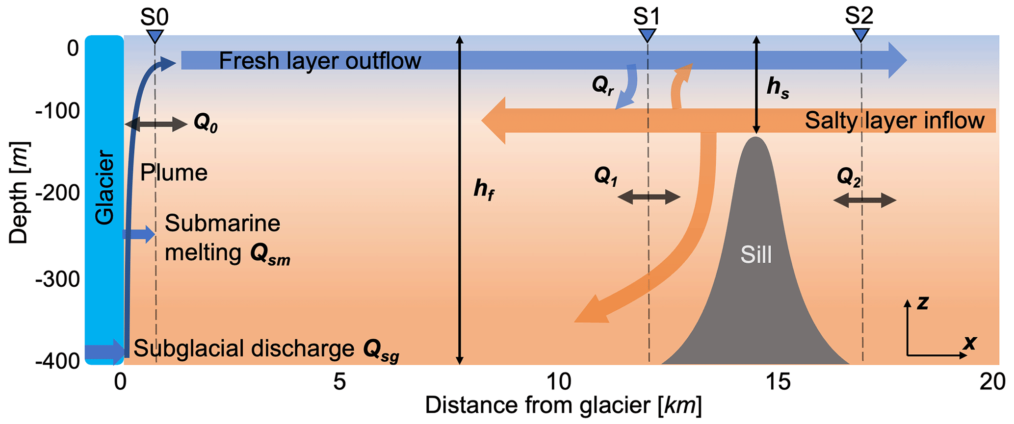
Figure 1Two-dimensional schematic (x,z) of the circulation and water properties in a glacial fjord. The flow in a fjord of depth hf is constrained by a sill with a shallowest depth of hs. Cross-sections for analysis are defined near the glacier front (S0) and on either side of the sill (S1, S2). Q0, Q1, and Q2 are volume fluxes through the sections and in the vertical (Qr).
To investigate the response of fjord circulation and submarine melting to variations in forcing and fjord geometry, we set up the plume–ocean fjord model in a domain with one Gaussian-shaped sill near the mouth (Fig. 1). The sill has a fixed width of 4 km and a shallowest depth of hs, which is varied in our simulations to examine the role of sill depth in modulating fjord circulation and heat supply to the glacier. The fjord domain is set to 2 km wide to limit the scope of our study to a reasonable set of parameters. While relatively narrow, we will show that this does not prevent the generation of significant cross-fjord variability in the circulation. The maximum depth of hf is 400 m in most cases, with a handful of cases using 200 m to test our results in a broader parameter space. The fjord is 20 km long and opens to a shelf region (27 km long, 16 km wide, and 400 m deep), with open boundaries at the north, south, and east edges. The cross-fjord grid spacing is 200 m inside the fjord, linearly increasing to 1 km at open boundaries. The along-fjord grid resolution ranges from 20 m at the sill to 100 m at the rest of the fjord, also linearly telescoping to 1 km at open boundaries. The vertical grid size of the model domain increases from 2 m at the free surface to 6 m at the bottom.
Table 1Summary of fjord geometry, initial conditions, and forcing conditions used in 93 model runs analyzed. hs: maximum sill depth; hf: maximum fjord depth; Qsg: subglacial discharge; Tini: initial fjord temperature; : initial fjord stratification; Cd: quadratic bottom friction coefficient; U0: tidal amplitude at the eastern open boundary. The linear stratification profile corresponds to values ranging from 0.5 to 4 × ( = 7.36 × 10⁻⁵ s−2).
The variables changed (geometry as well as initial and forcing conditions) for different runs are listed in Table 1. The initial fjord conditions are horizontally homogeneous, with temperature and salinity profiles restored at open boundaries on the shelf throughout the simulation. We changed the size of the shelf and found no significant difference in our results, suggesting that they are not impacted by these boundary conditions. The initial water temperature is a constant ranging from 2 to 10 ∘C. Most runs used an idealized initial salinity based on a Greenland fjord profile (Cowton et al., 2015), where the salinity ranges from 32 to 33.8 in the upper 80 m and slowly increases to 34.5 at the bottom (“Idealized” in Table 1). To further explore the impact of varying stratification, we also set up a set of experiments with a linear salinity profile that increases from 23 on the surface to 27 at the bottom with a stratification of s−2 defined as . With a fixed mid-depth salinity, the gradient and thus the initial ambient stratification range from to . Initial velocities are zero throughout the domain except for tidal simulations. For runs that include tidal forcing, a uniform zonal velocity is applied along the eastern boundary (the fjord is oriented east-west) of the model domain Ut=U0sin (ωt) at the M2 tidal period ((12.42 h); t is time), where the velocity amplitude U0 ranges from 0.01 to 6 cm s−1 to generate weak to strong tides relative to the subtidal exchange flow at the sill. The Coriolis parameter is set to s−1. The K-profile parameterization (KPP) scheme (Large et al., 1994) is used to parameterize vertical mixing. A quadratic bottom drag parameterization with a coefficient of was used for most runs. A small set of simulations were run using a drag coefficient of , , and to test the impact of varying bottom drag. Those runs are not shown, but changing the drag coefficient did not meaningfully impact our results.
We used passive tracers (MITgcm PTRACERS package) to estimate the timescales of the response of the fjord to changes in shelf properties. For this purpose, a first tracer with a constant concentration was introduced at the entire shelf region, and a second tracer was injected into the same region, but its concentration increases with time at a fixed rate. Then the ratio of these two tracers in any model grid is used to estimate the “age” of the shelf water tracer at that location (e.g., Rayson et al., 2016; MacCready et al., 2021).
We emphasize, however, that both the dynamics of the fjord circulation and the dynamical response of the submerged glacier terminus to ocean forcing are complex. Studies have shown, for example, that the formation of cavities in the ice can significantly change the rates of submarine melting, driving higher-than-predicted melting (Jackson et al., 2017) and that existing melting parameterizations underestimate the observed background melting rates (Jackson et al., 2020). Our choice of simplified sill is meant to understand the role of bathymetric constrictions on the flow, including enhanced mixing. In real fjord systems, enhanced mixing could also be promoted by other bathymetric features, multiple sills, icebergs (Hager et al., 2023), or other factors. This complexity is not well represented in our simplified model, but our setup is still a useful guide to exploring the dynamics of ice–ocean interactions in systems with shallow sills.
We analyzed 93 model runs where we varied the sill depth hs, subglacial discharge Qsg, initial fjord temperature Tini, stratification , bottom drag Cd, and tidal forcing (Table 1). The shallowest sill depth hs is nondimensionalized by dividing by the maximum fjord depth hf, and this depth ratio varies from 0.04 to 0.12 to characterize shallow-silled fjord systems, e.g., in Alaska (Motyka et al., 2013; Love et al., 2016) and Patagonia (Moffat et al., 2018). Cases without sill () are included to understand the overall impact of the sill. The subglacial discharge flux Qsg is varied in the range 25 to 1000 m3 s−1 to cover different magnitudes of freshwater forcing and to represent the seasonal variation of runoff, although we recognize that the high end of this range is likely unrealistic given the size of our domain. All simulations are run for 60 d, in which most runs reached a near-steady state, where key aspects of the circulation (e.g., exchange flow) and water properties (layer thicknesses, heat storage) did not change meaningfully with time.
2.2 Total exchange flow and efflux–reflux calculations
The exchange flow along the fjord is calculated using the total exchange flow (TEF) method (MacCready, 2011). Transports through a cross-fjord section are sorted into salinity classes, tidally averaged, and then integrated vertically and across the fjord. The inflow volume flux Qin is the sum of the transport in all inward-flowing salinity classes, and the flux-weighted salinity of the inflow is Sin. Similarly, the outflow is quantified as Qout and Sout. The TEF method decomposes salt flux in salinity space instead of physical space, yielding the exchange flow that incorporates both tidal and subtidal processes and satisfies the Knudsen relation precisely (MacCready, 2011). TEF has been used extensively in estuarine systems (Geyer and MacCready, 2014; Wang et al., 2017; MacCready et al., 2021).
To apply the TEF method, the volume transport through each cross-section is binned with salinity output stored every 6 h, using 1000 bins between 0 and 35. After tidally averaging (for runs where tides are included), the transport at each time is divided into inflowing and outflowing components according to the dividing salinity method (MacCready et al., 2018). Integrating transport in glacierward or oceanward components gives us Qin and Qout. Similarly, integrating the transport times the salinity of each bin in the two directions gives the inflowing and outflowing salt flux. Then Sin and Sout are derived from dividing the salt flux by the volume flux in the same direction. Based on steady-state volume conservation, the entrainment flux (downward reflux) Qr across the upper-bounding isohaline surface equals the divergence of inflow or outflow through the segment bonded by two cross-sections (Wang et al., 2017).
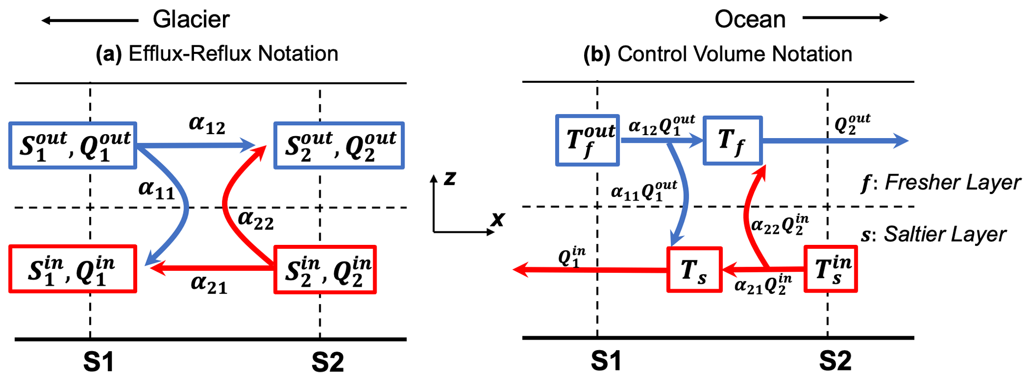
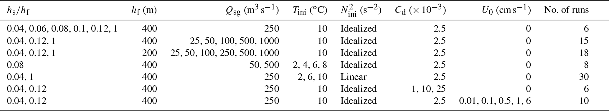
Figure 2Notations of (a) efflux–reflux calculation and (b) a control volume. The segment between sections S1 and S2 has a fresher layer and a saltier layer in the vertical. Temperature, salinity, and volume fluxes are denoted by T, S, and Q. αfrom,to represents the efflux–reflux fractions (e.g., α12 signifies the efflux–reflux fraction from section S1 to section S2). Figure modified from Fig. 7 in MacCready et al. (2021).
To estimate and quantify the vertical exchange between the upper and lower layers, we utilize the efflux–reflux formalism that was first developed in Cokelet and Stewart (1985) and has been applied to both estuary and glacial fjord studies (MacCready et al., 2021; Hager et al., 2022, 2023). In its simplest form, the efflux–reflux theory defines a channel segment between two cross-fjord sections with a steady two-layer exchange flow and known salt and volume transports through the cross-sections on either side (Fig. 2a). For the flow from any incoming layer, the reflux fraction corresponds to independent upward and downward turbulent transports across the segment, while efflux is the fraction that continues moving into the next reach. The reflux fraction therefore expresses the vertical fluxes as volume transports, which is equivalent to the horizontal fluxes in TEF. All transports are positive; the two cross-sections (S1 and S2) connect three segments, each of which has two layers in the vertical, a shallow fresher one and a deep saltier one. Following Cokelet and Stewart (1985), the system of equations to be solved is
The efflux–reflux coefficients α are then determined by solving the matrix equation based on the conservation of volume and salt, and the sum of efflux and reflux fractions should be equal to unity, that is, . In this framework, the vertical exchange components that we are primarily concerned with can be solved as
Combining efflux–reflux fractions and TEF transports, a control volume can be defined for layer temperature along the fjord (Fig. 2b). It is also bounded by two cross-fjord sections S1 and S2, with no exchange at the sea surface. A third section (S0) is defined to understand the near-glacier properties and circulation. The layer interface throughout the control volume is determined by the zero-crossing point of the along-channel velocity profile, which assumes a two-layer exchange. Following the notation in Fig. 2b, the equation for the temperature of the lower (saltier) layer with a volume of Vs can be expressed as
At steady state (), the expression of the lower-layer temperature becomes
We can use the reflux part (α11,α22) of the efflux–reflux together with the TEF calculations to determine both horizontal and vertical transports and deep-layer temperature in the control volume. As we will show later, the exchange flow at the sill might be of secondary importance to water modification and exchange occurring elsewhere, or the exchange flow might have three layers, and thus we are limiting the use of this approach only to cases where there is a well-defined two-layer exchange flow at the sill.
Figure 3Time-mean (averaged over the last 14 d of simulations) potential temperature anomaly (with respect to an initial temperature of 10 ∘C). All cases have Qsg = 250 m3 s−1, and sill depth varies from (a) , (b) , and (c) . The red-outlined areas are zoomed in on the right panels, with vertical velocity scaled up by a factor of 15. Black contours denote water density anomaly; Qsm is the volume flux of submarine melting.
3.1 Base case: first-order impacts of a shallow sill
To illustrate the first-order impact of the sill on fjord–shelf exchange in our runs, we present a base case driven by thermal forcing and subglacial discharge in fjords under varying sill depths. Qsg is set to 250 m3 s−1 and drives the formation of a buoyant plume, entraining ambient warm water while rising vertically along the glacier front. This entrainment into the outflowing plume is balanced by a return flow of warm oceanic water at depth. The fjord reached a steady state in about a week. We vary the sill–fjord-depth ratios from 0.04 to 0.12 to characterize the impact of shallow sills on mass exchange between the fjord and the shelf, as well as the cooling of deep oceanic water across the mouth of the fjord (Fig. 3).
Increasingly shallow sills create strong mixing there, resulting in the cooling of the warm oceanic layer flowing toward the glacier. With no sill and the plume reaching the surface (, Fig. 3a), the outflow occupies the top 40 to 45 m of the water column in the fjord interior, and, as expected, the exchange between upper and lower layers, Qr, is negligible. As the sill depth shallows (, Fig. 3b and c), a front with increasingly steeper isopycnals and stronger flow develops as the oceanic inflow accelerates over and down the slope after crossing the sill. Strong mixing is observed in this region and results in the upper-layer outflow recirculating before passing the sill, cooling the deep fjord as a result. In these shallow sill cases, the lower-layer inflow cools by 0.2 to 1 ∘C as it moves from the shelf to the fjord interior. The cooling of deep fjord water is most significant above ∼ 350 m.
The increased mixing with shallower sills in these two-layer cases is consistent with well-understood fjord dynamics where the flow over the sill can reach a supercritical condition that enhances downstream mixing (Geyer and Ralston, 2011). Layer-averaged along-fjord velocity and layer salinity are defined as Uupper, Ulower, and Supper, Slower, respectively. The Froude number, which is greater than 1 when the flow is supercritical, is
where is the reduced gravity, and ρ and h denote the density and thickness of the upper and lower layers. In the base case simulations, the upper-layer outflow remains subcritical, while the lower-layer Froude number reaches criticality as falls below 0.06, indicating hydraulic control. The cooling of deep water that results from the enhanced mixing and reflux over the sill can be diagnosed using Eq. (4) (Fig. 5). With a minor (< 4 %) adjustment to the downward reflux coefficient α11, the theory predicts the deep-water temperature with a coefficient of determination of r2=0.99. Both estimated and modeled results show that the deep fjord is 0.1–0.6 ∘C colder than the shelf water, with shallower sills resulting in greater cooling (Fig. 5).
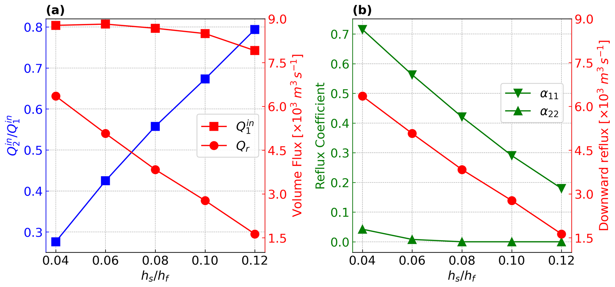
Figure 4TEF transports (a) and reflux fractions (b) with varying sill depths. 1 and 2 denote the cross-fjord section on either side of the sill, and denote the volume fluxes of the water flowing into the fjord, Qr denotes the downward reflux, and α11 and α22 correspond to downward and upward reflux fraction, respectively.
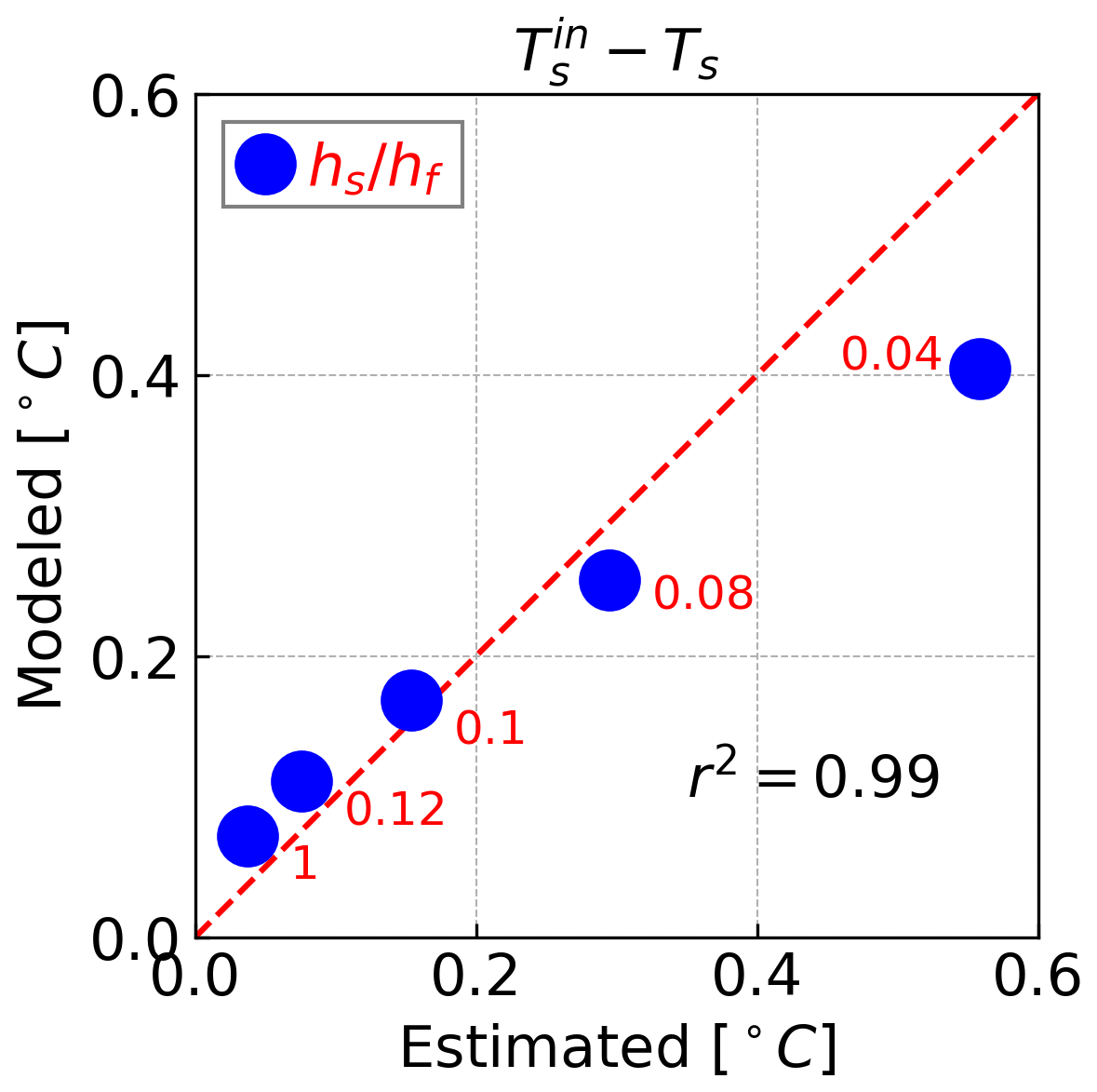
Figure 5A comparison between the deep-water temperature anomaly () estimated from Eq. (4). is the temperature of incoming oceanic water from the shelf. The reflux coefficient α11 is scaled up by 3.5 %; results are averaged over the last 14 d of simulations.
While the volume transport from the ocean outside the fjord () is drastically reduced when the sill is shallower, this reduction is largely compensated for by the increase in reflux into the incoming layer (Qr). The near-mouth exchange fluxes in the shallowest-sill case (, Fig. 4a) are approximately 64 % smaller than the no-sill case. As decreases from 0.12 to 0.04, the downward volume transport Qr increases by a factor of ∼ 3. Across the shallow sill cases, the deep incoming transports in the fjord near the sill (, Fig. 4a) and near the glacier (not shown) remain largely unchanged as a result of the increased sill-driven reflux. That is, while a shallow sill does result in strong cooling and reduction of the inflow of oceanic water, it does not significantly change the strength of the circulation within the fjord itself. As the sill becomes shallower, the downward fraction α11 increases nearly linearly and is consistent with the variation of reflux Qr. As decreases from 0.12 to 0.04, Qr increases by about 5000 m3 s−1, and at least 50 % more of the outflowing water is refluxed into the deep layer. The upward reflux coefficient α22 is close to zero in all these cases (Fig. 4b).
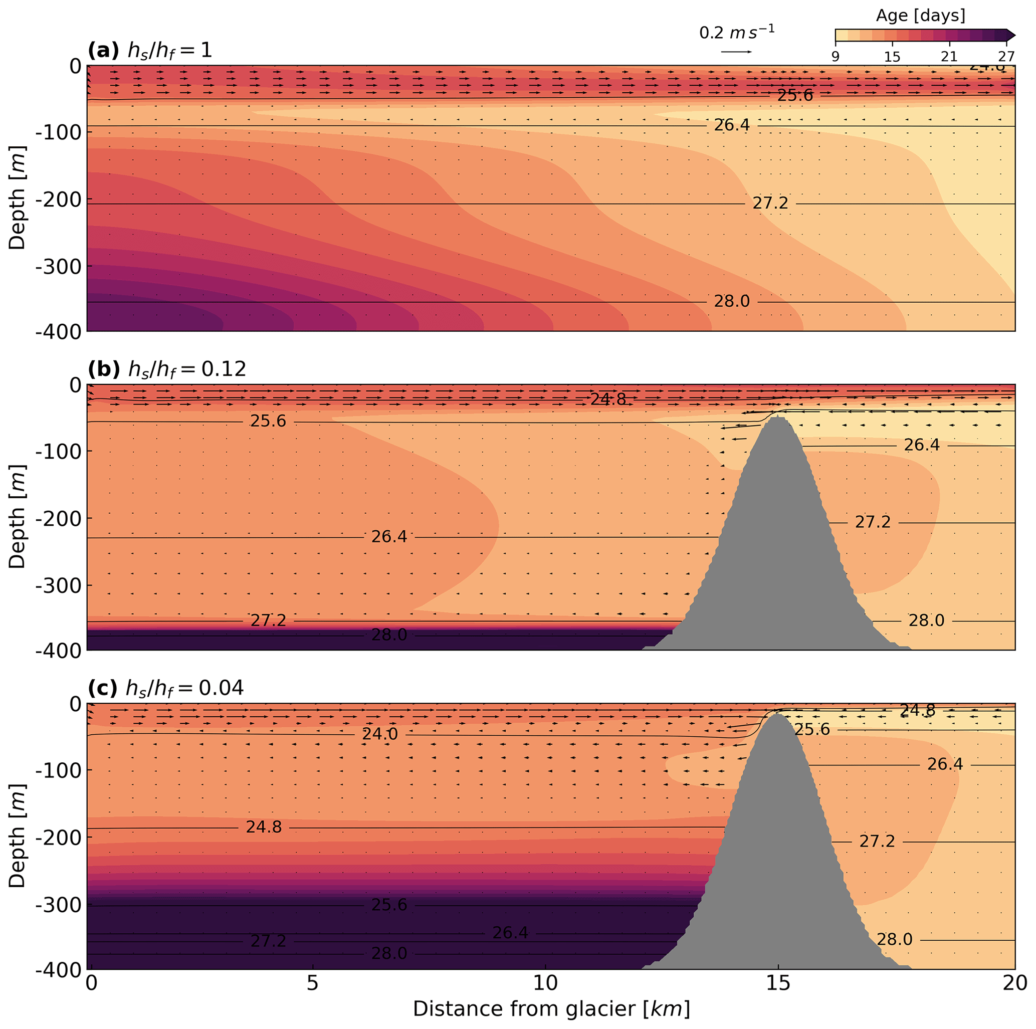
Figure 6Along-fjord distribution of the shelf water tracer age at the end time (day 60) of simulation. Qsg = 250 m3 s−1; black contours denote water density anomaly.
The presence of the sill also impacts the response timescale of the fjord to shelf variability (Fig. 6). The tracer age increases, as expected, with depth and distance from the shelf, and the shelf water takes less than 23 d to reach the entire fjord when there is no sill (Fig. 6a). As the sill becomes shallower and mixing near the sill increases, the maximum intrusion depth in the fjord decreases as more of the lighter outflow is entrained into the inflowing oceanic water. When comparing the velocity and density profiles in Fig. 6b and c, the intrusion depth of shelf water decreases from about 350 m to 250 m as the sill ratio is reduced from 0.12 to 0.04. Consistent with circulation patterns, the tracer age is much lower within the incoming flow than within the near-bottom layer.
3.2 Circulation and cooling regimes
The base run discussed in Sect. 3.1 illustrates the case where the resulting fjord circulation closely resembles a typical shallow-silled fjord (i.e., without a marine-terminating glacier), where a two-layer exchange flow is formed and strong control on the exchange is exerted by the sill. However, a key difference is that adding a deep source of buoyancy at the head of the fjord results in significant subsurface mixing and cooling of the lower layer. A buoyant plume formed by injection of freshwater at depth and rising through a stratified fluid can result in the plume reaching neutral buoyancy well below the surface. Strong stratification can constrain the plume terminal height and thus reduce the distance from the plume detachment location at the glacier, and it also impacts the overall entrainment of warm ambient water, reducing submarine melting. In this section, we focus on how these subsurface plumes interact with a shallow sill and how the changes in stratification compete with the cooling to modulate the modeled submarine melting rates.
A scaling for the height hp that a plume generated by a point source of subglacial discharge reaches can be estimated from (Slater et al., 2016)
Based on buoyant plume theory (Morton et al., 1956), the terminal depth depends on the reduced gravity of the plume g′, denoted as it was evaluated at the grounding line with the fresh plume density and a reference density. It also depends on the entrainment coefficient γ, here taken to be 0.1, and the ambient stratification . h0 is a nondimensional height related to the radius, velocity, and reduced gravity of the plume. We estimated h0 from five runs with Qsg = 250 m3 s−1, using a fixed temperature (10 ∘C) and an initial salinity increasing linearly in the vertical with a range that represents weakly to strongly stratified glacial fjords. Fitting the results to Eq. (6) resulted in an empirical coefficient of h0=1.69 across this range of initial stratification conditions.
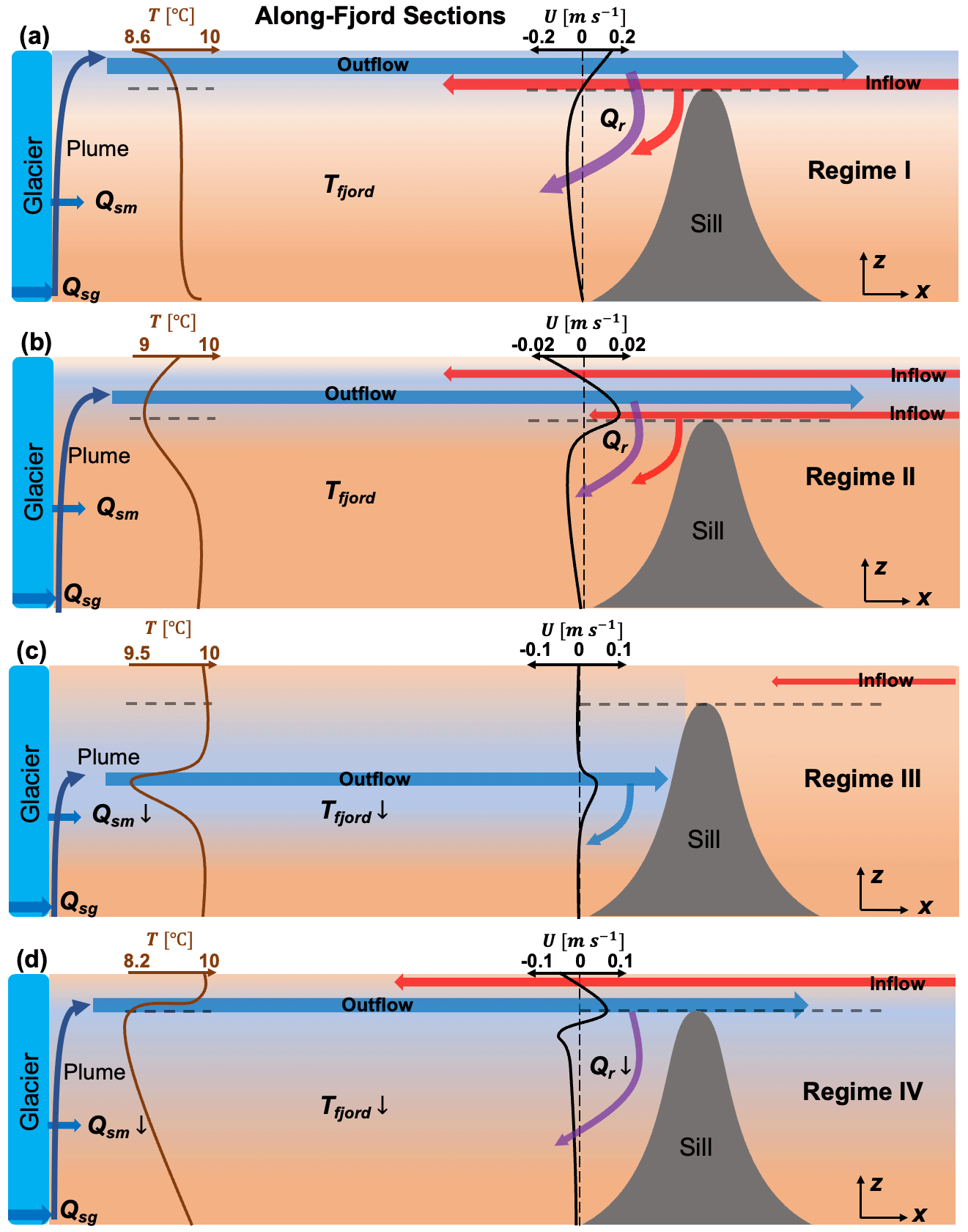
Figure 7Schematic of circulation regimes in shallow-silled glacial fjords. Brown and black curves are approximate temperature profiles near the glacier front and along-fjord velocity profiles on the glacierward side of the sill, respectively. Horizontal dashed gray lines indicate the maximum sill height. The colors of shades and arrows represent relative water temperatures. The sizes of the arrows indicate the relative magnitude of transports. Parameters depicted include subglacial discharge (Qsg), submarine melting (Qsm), deep-fjord temperature (Ts), and sill-driven reflux (Qr).
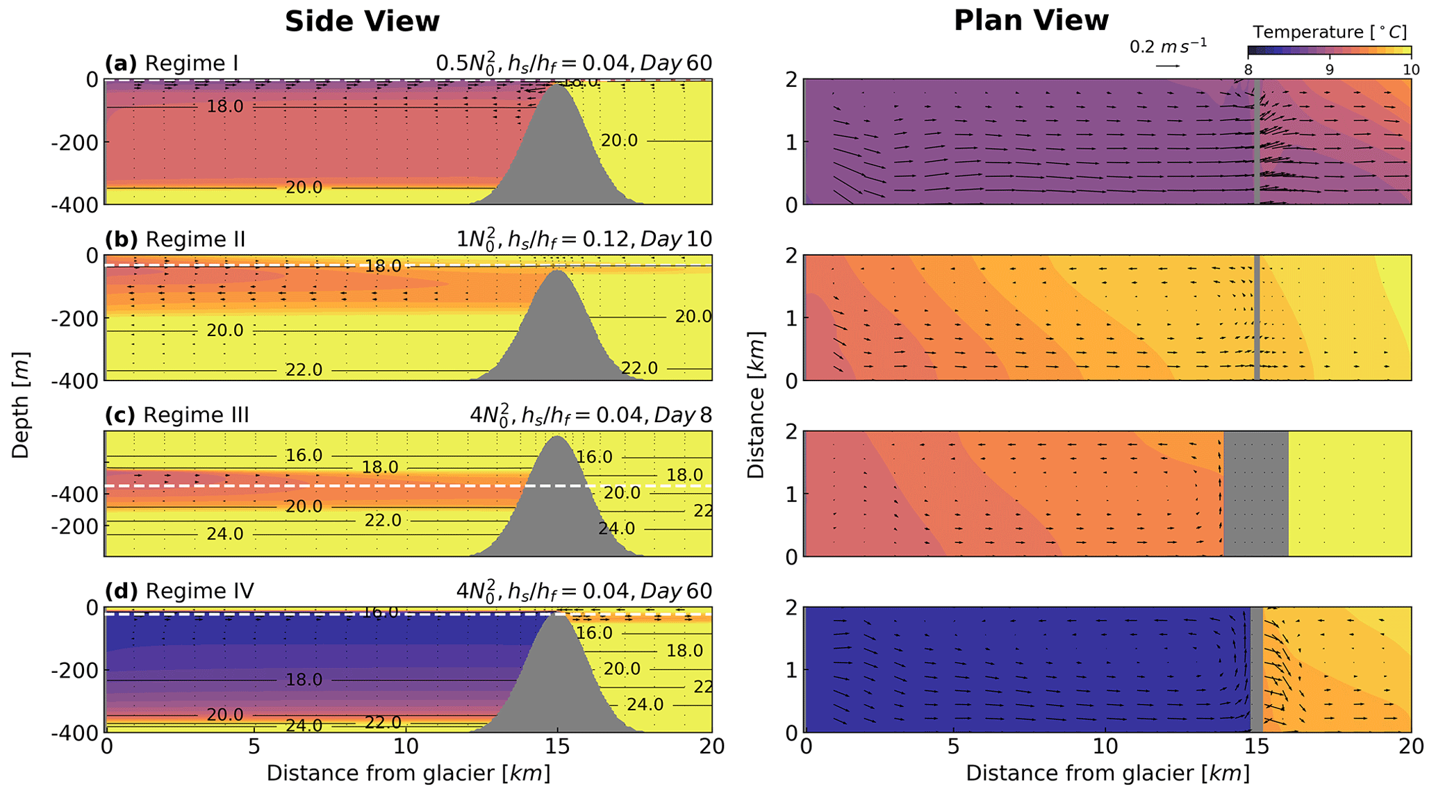
Figure 8Snapshots of fjord circulation regimes (a–d) from side (left panel) and plan (right panel) views Black contours denote water density anomaly, dashed white lines indicate the depths at which the plan-view snapshots are taken, and gray-shaded areas represent sill locations. Across-fjord structures of the regimes can be found in Figs. S1 and S2 in the Supplement.
The relative depth of the fjord hf, the sill hs, and the initial height of the plume hp (Eq. 6) help define four circulation regimes that were evident in our model runs. These are shown schematically in Fig. 7 and further illustrated by model snapshots in Fig. 8. When the initial stratification is relatively weak or the subglacial discharge is relatively strong so that the plume reaches fjord surface and , the circulation is characterized by the near-steady, two-layer exchange flow that we described in the base case, where hydraulic control and the reflux of the cold outgoing plume water into the lower layer are the dominant processes controlling the cooling of the lower-layer temperature (Regime I, Figs. 7a and 8a). When (i.e., a subsurface plume) and (i.e., the plume depth is above the sill) a three-layer circulation regime is formed, with a subsurface freshwater overlying oceanic inflow into the fjord (Regime II, Figs. 7b and 8b). In our runs, the surface layer above the outgoing plume showed a rather weak circulation, and Regime II was transient as the outgoing plume continued to mix and eventually reached the surface, i.e., transitioning to Regime I. However, this relatively fast transition might not generally be the case in fjords with deeper sills, relatively weak subglacial discharge, or relatively strong near-surface stratification. We note that as water properties and stratification evolve over time, the fjord circulation regime might shift, transitioning, for example, from Regime III to Regime I as the plume is initially trapped in the fjord before eventually rising to the surface.
The circulation regimes that lead to the strongest deep cooling are III and IV, that is, when . In these cases, the freshwater plume cannot exit the fjord, at least initially (Fig. 7c, d and Fig. 8c, d). Regime III shows the outgoing plume reaching the sill and forming a horizontal recirculation. Heat drawn from the deep fjord waters by submarine melting at the ice face and entrainment of warm ocean water into the outgoing plume cannot be replaced with exchange with the shelf, and thus the deep fjord continues to cool because the heat budget, in this case, is fundamentally unsteady. The subsurface (and sub-sill) plume continues to mix with the surrounding waters, rising in the process (Fig. 8c). Some, but not all, of our Regime III cases eventually reached the sill depth during our 60 d runs, allowing the plume to exit the fjord and thus forming a last distinct circulation, Regime IV. In this configuration, the circulation resembles a reverse estuary, where the exchange is either lateral or vertical (Fig. 8d), but outflow is concentrated just above the sill. However, this regime is also fundamentally unsteady because heat entrained into the outgoing plume from the deep water in the fjord cannot be readily replaced with exchange with the shelf, leading to continuous cooling of that layer as well.
In Regime III cases, the plume remains trapped below the sill for periods ranging from a few days to the entire 60 d run, suggesting that this process might be relevant for understanding seasonal-scale changes in fjord circulation and melting regimes. We can approximate this problem by assuming that the fjord below the sill acts as a “filling box” (Baines and Turner, 1969), where the outflowing plume progressively fills the basin downward from the initial level of neutral buoyancy. Cardoso and Woods (1993) provided an estimate of the timescale ta for a horizontal plume in a linearly stratified environment to ascend (or “fill the box”) as
where is a characteristic length scale (Morton et al., 1956) proportional to the initial plume height hp in Eq. (6), A is the horizontal cross-section area from the glacier front to the sill, and is the buoyancy flux of the plume. This approximation assumes that the contribution to B from submarine melting is negligible. The nondimensional time τ can be obtained from
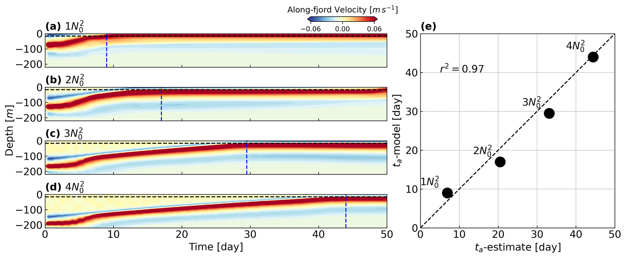
Figure 9Ascending time (ta) of the plume with increasing initial stratification. (a–d) Evolution of the vertical structure of along-fjord velocity near the glacier front, with positive values toward the fjord mouth. Horizontal dashed black lines show the maximum sill height (), and vertical dashed blue lines indicate the estimated time for the plume rising from its initial height to the level of the sill crest. (e) A comparison between the plume ascending time estimated from theory and the model output.
As the initial plume height hp decreases with the prescribed initial stratification increasing from to , the plume takes longer to reach the crest of the sill (Fig. 9a–d). Equation (7) gives a reasonable estimate of the timescale for the plume rising to the sill level and leaving the fjord (Fig. 9e), ranging from less than 10 d to about 6 weeks. While the initial stratification leading to these estimates is prescribed, this suggests that Regime III cases can last for a significant period.
In summary, we find that for cases where the circulation regime is dominated by a two- or three-layer exchange flow above the sill depth (Regimes I and II), with inflow from the ocean at depth, the dynamics of sill-driven mixing and reflux discussed in the base case are critical to understanding how deep-fjord properties will evolve. In these cases, a steady view of the circulation in at least seasonal timescales is reasonable, as deep heat supply from the shelf balances the heat loss due to mixing and melting (Figs. S3 and S4 in the Supplement). When strong stratification or weak subglacial discharge results in an outflowing plume that is deep relative to the sill, as in Regime III, cooling of the deep fjord is not caused by sill-driven advection and mixing but by the continuous removal of heat from the deep layer of the fjord that cannot be replaced by an oceanic inflow. Critically, this means that the properties in the fjord can be strongly time-dependent in synoptic to seasonal timescales, and sill processes become less important until the plume reaches the sill crest.
3.3 The competing impacts of deep stratification and temperature changes on submarine melting
While the sill restricts the inflow of warm oceanic water to the fjord and reflux from the freshwater plume results in cooling of the deep water near the glacier, submarine melting is often larger in runs with shallow sills compared to equivalent no-sill runs. Submarine melting (Qsm) was slightly higher with shallow sills in our base case (Fig. 3) and consistently so in the cases discussed in Sect. 3.2, where Qsm decreased for all cases as the linear stratification increased, but it was also lower for the no-sill cases (, Fig. 10).
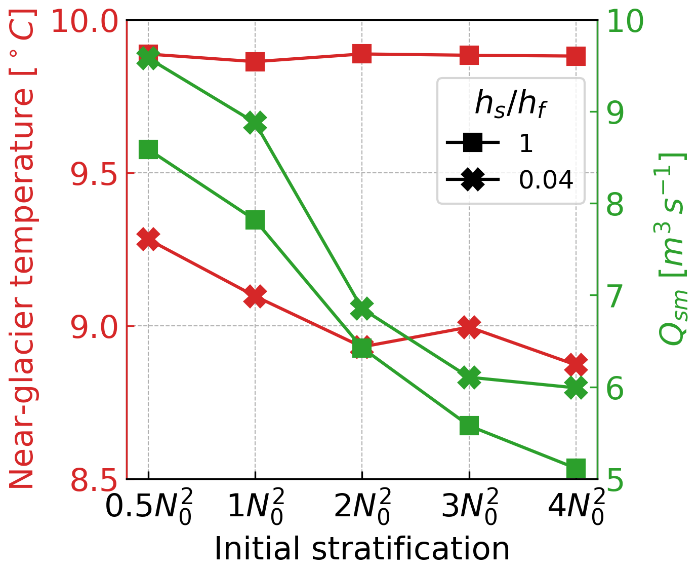
Figure 10Impact of shallow sill vs. fjord stratification on near-glacier temperature and submarine melting; results are averaged over the last 14 d of each simulation.
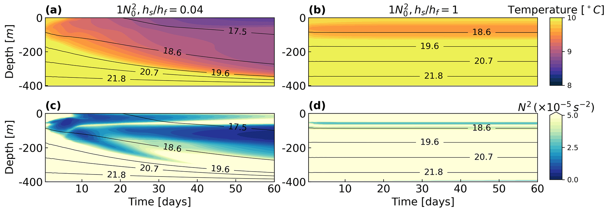
Figure 11The evolution of near-glacier temperature (a, b) and near-glacier stratification (c, d) at S0 (near the glacier) with (a, c) and without (b, d) a sill. Forcing and initial conditions other than the sill depth are the same.
The perhaps counterintuitive result of submarine melting increasing as deep cooling is enhanced by shallow sills can be understood by considering that sill processes also decrease stratification, which has the opposite effect on submarine melting. This competition is illustrated in Fig. 11, which shows the evolution of near-glacier temperature and stratification for two cases with the same initial and forcing conditions other than the presence of a shallow sill. But for a brief period at the start of the shallow sill run (Fig. 11a and b), both cases are examples of Regime I, where a surface outflow is generated. When there is no sill (), the melting (Fig. S5 in the Supplement), fjord temperature, and stratification remain nearly constant throughout the simulation (Fig. 11b and d). With a shallow sill (), however, cooling is overwhelmed by the collapse of stratification in the deep water to increase submarine melting, particularly after 30 d or so (Fig. S5 in the Supplement). During that period, the fjord temperature dropped as expected from the cooling effect of sill-driven reflux (Fig. 11a). Meanwhile, the fjord stratification became significantly weaker due to strong mixing with the refluxed plume outflow and the sill impeding the inflow of denser shelf waters into the fjord (Fig. 11c).
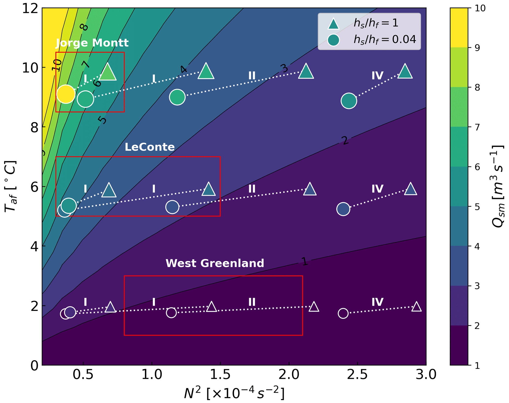
Figure 12Dependence of submarine melt on fjord stratification and thermal forcing with a constant subglacial discharge of Qsg = 250 m3 s−1. Cases with the same initial temperature (2, 6, 10 ∘C) and stratification (, , , ) but no or shallow sill are connected by dotted white lines. The sizes and colors of the markers represent the magnitude of Qsm for each run. The background contours correspond to the scaling of Qsm based on with an added proportionality constant calculated from the model output (Fig. S6 in the Supplement). The results are averaged over the last 14 d of each simulation, corresponding to circulation regimes determined by initial stratification ( and : Regime I; : Regime II; : Regime IV). The red boxes highlight approximate observed ranges of glacial fjord properties from Patagonia (Jorge Montt; Moffat et al., 2018), Alaska (LeConte; Jackson et al., 2022), and West Greenland (e.g., Mortensen et al., 2011; Gladish et al., 2015).
The competition between the decrease in stratification and cooling driven by the presence of the sill is further illustrated in Fig. 12, which shows Qsm as a function of initial stratification and fjord temperature. Qsm is proportional to , where is the divergence between the modeled ambient temperature Ta and the freezing temperature of seawater T0 (Slater et al., 2016). We used a linear fit (Fig. S6 in the Supplement) to find the constant of proportionality between the modeled Qsm and the scaling above. Several runs with constant initial and forcing conditions, but where a shallow sill is added, are shown here; the markers are color-coded with the magnitude of the modeled Qsm.
Consistent with Fig. 11, the results indicate that the lowering of deep-water stratification caused by the presence of the sill has an equal or greater impact on submarine melting than the cooling that occurs there. We note that we ran no-sill cases only for a subset of our sill runs. Fjords where adjacent deep waters are warm with relatively low stratification (e.g., Jorge Montt in Patagonia) might be an example of this outcome, while Greenland fjords where the ambient waters are relatively cold might be less so. From considering the relative changes to with respect to N2 and Taf, we would expect that the change in deep temperature ΔTaf (i.e., the change in deep temperature across the sill caused by the presence of the sill) must exceed to generate a net increase in submarine melting. And ΔN2 is the equivalent and competing change in stratification across the sill.
Our results indicate that the impact of shallow sills on submarine melting in glacial fjords depends on the competition between cooling and the decrease in stratification caused by the presence of the sill. The only source of these changes in deep-water properties is the interaction between the sill and plume-driven circulation. The impact of tidal currents, which can be an important source of mixing in fjords, is briefly explored next.
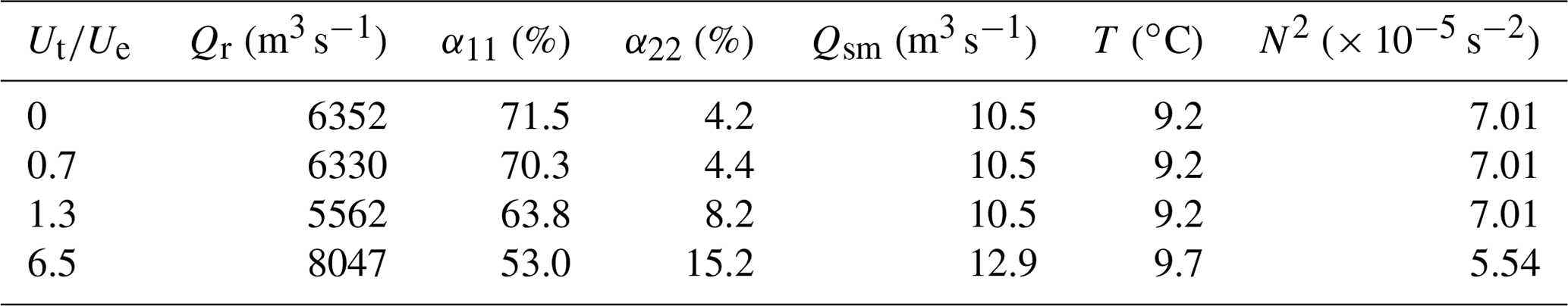
Table 2Tidal–exchange-velocity ratio (), downward reflux over the sill (Qr), downward reflux fraction (α11), upward reflux fraction (α22), submarine melting (Qsm), mean temperature (T), and stratification (N2) near the glacier front for tidal experiments with Qsg = 250 m3 s−1 and .
3.4 The impact of tides
Tides are another important process that modulates the circulation and mixing rates in fjords. We ran 10 additional simulations with a shallow sill configuration () and varying tidal amplitudes at the eastern boundary of the model (see Sect. 2) to force a range of tidal velocities at the sill (Ut) relative to the exchange flow Ue. Ut is estimated at the sill from harmonic analysis (Codiga, 2011). Ue is estimated from
where Qe is the exchange flow transport defined as , Qin and Qout are positive, and Asill is the cross-channel area at the sill crest. In the tidal simulations, Ut ranges from 0.1 to 1 m s−1, and Ue is nearly constant, ranging from 0.13 to 0.15 m s−1. The sill-driven reflux Qr, deep-fjord temperature Ts, and submarine melting with and without tidal forcing are summarized in Table 2. The results are averaged over the last 14 d of simulations.
Increasing tidal forcing leads to a reduction in the downward reflux fraction and an increase in the upward reflux fraction, with varying impacts on the downward reflux Qr. The outflow increases with stronger tidal forcing due to enhanced exchange flow along the fjord, particularly as the tidal velocity exceeds the exchange velocity (). The increase in the upward reflux fraction (α22) with tides reflects enhanced vertical exchange. A small (5 %) increase in melting is evident for the weakest tidal forcing case relative to the no-forcing case. For tidal cases with between 0.7 and 1.3, the small changes in reflux magnitude did not have a meaningful impact on the stratification, deep-water temperature, or submarine melting. The strongest tidal forcing case we ran did result in the weakening of stratification and a warmer fjord compared to the other cases (Fig. S7 in the Supplement), which is reflected in the highest melting rate. The warm outflow in this case is also enhanced by the upward entrainment flux and gets largely (> 50 %) refluxed into the deep fjord. Overall, the decrease in the reflux fraction is consistent with the results from Hager et al. (2022), but fully understanding the impact of tidal forcing in these systems requires further study.
4.1 Application to realistic fjord systems
The sill reflux process described above has been discussed in observational studies in both non-glacial and glacial fjords. In Loch Sunart, a shallow-silled Scottish fjord, hydrographic and current meter data collected during the summers of 1987, 1989, and 1990 revealed that an estimated 20 % to 70 % of the surface water recirculated into the bottom layer (Gillibrand et al., 1995). At Godthåbsfjord, Greenland, the summer surface water in the sill region was observed to reach the glacier terminus at depth, with the subsurface freshwater fraction increasing from winter (3 %) to summer (10 %) (Mortensen et al., 2013). The authors highlighted a mixing process at the sill that resembles the reflux of glacial freshwater that we focus on here. Most recently, observations in LeConte Bay, Alaska (), showed that 50 % to 75 % of the summer inflow was composed of refluxed plume-driven outflow (Hager et al., 2022). This range is comparable to our base case simulations (Fig. 4b).
The circulation regimes identified here (Fig. 7) suggest that conceptual models of glacier melting where the circulation and heat budget of the fjord are steady might not always be adequate. When a buoyant plume flowing away from the glacier is blocked by the sill (Regime III) or barely reaches the sill level (Regime IV), the system is temporarily unsteady as the plume continues to rise, and the deep water below is cooled. During the summer, glacial fjords in Greenland (Mortensen et al., 2013), Alaska (Hager et al., 2022), and Patagonia (Moffat et al., 2018) show intense subglacial discharge and surface or subsurface plume outflow as in Regimes I and II (Fig. 7a and b). With stronger ambient stratification or weaker winter subglacial discharge, buoyant plumes enter the fjord at depth, forming an outflow that intersects the sill or is mostly blocked by it (Gladish et al., 2015; Carroll et al., 2016), resembling Regime III (Fig. 7c), in which case the blocked outflowing plume is expected to progressively cool the deep fjord. In the fall–winter circulation regime at LeConte Bay, Alaska (Hager et al., 2022), the reduced freshwater outflow could be blocked by a shallow sill, recirculated as in Regime III. In that system, however, strong tidal currents also play an important role in exchange across the sill. We were unable to find published reports on Regime IV (Fig. 7d), perhaps because this circulation could quickly transition to Regime II or I. Because Regimes III and IV reflect an unsteady state for the temperature and stratification of the fjord, both of which impact the melting rate, caution should be used when applying a melting parameterization that assumes a steady fjord circulation.
Our simplified model configuration ignores what are possibly key processes that modulate both the reflux process and its impact on the heat supply to the ice. While we briefly explored the tidal variability, the reason for the reduction of the reflux fraction under stronger tidal currents, also reported by Hager et al. (2022), is not well understood. Wind forcing is a well-known factor influencing the exchange between glacial fjords and the open ocean (Straneo et al., 2010; Jackson et al., 2014; Moffat, 2014). Finally, we did not fully explore how more realistic shelf properties, multiple sills, or different fjord widths could influence the processes investigated here. However, we believe that the regimes discussed above still provide a useful framework to move forward.
4.2 Implications for glacial melt
Our results show that the downward transport of outflowing glacial freshwater at the sill cools the fjord, which is consistent with previous studies. Although the sill–fjord-depth ratio has a significant impact on the downward reflux fraction (Fig. 4b), the magnitude of reflux and thus the warm water supply to glaciers are largely determined by the strength of subglacial discharge, especially with a shallower sill. Depending on the properties of the outflow, the sill-driven reflux may have reduced or increased heat transport to the glacier. For example, numerical experiments by Hager et al. (2022) found that the warmest surface water during the summer was refluxed and transported to the terminus of the LeConte Glacier, enhancing heat supply and submarine melting.
One key result from our study is that the presence of a sill leads to a decrease in both temperature and stratification of the deep inflow, with opposing effects on the rate of submarine melting. In our simulations, the stratification effect is generally greater than the cooling effect, leading to higher submarine melting for shallow sill cases. However, several caveats should be noted: first, our results depend on the erosion of fjord stratification that is prescribed as an initial condition – the same as for the outside shelf, for convenience, rather than the result of a more realistic evolution. The underlying assumption is that the fjord stratification is changing, for example, from winter to summer, and is set before the onset of a large change in the subglacial discharge, but that evolution is not modeled explicitly. Second, the temperature structure we use is rather simple to keep the parameter space reasonable, but it is common to observe multiple distinct deep-water masses outside glacial fjords. For example, a shallow sill might favor overall warmer waters entering the fjord, as it happens in Jorge Montt fjord, where a subsurface temperature maximum is found at about sill level outside the fjord (Moffat et al., 2018). Despite this complexity, our results highlight the importance of understanding the processes controlling not only deep-water temperature but also stratification in these systems.
Ambient melting is likely too small in our study, given that observations show that it can be a significant fraction of the total submarine meltwater flux (Jackson et al., 2020). Modeling shows that these background melt plumes also entrain fjord waters and intrude into the fjord after reaching neutral buoyancy (Magorrian and Wells, 2016). The coefficients used in submarine melt parameterization are derived from studies on ice shelves (Cowton et al., 2015), so the dynamics and morphology in the near-ice zone could be substantially different in tidewater glaciers (Jackson et al., 2022). Estimates of near-glacier fjord circulation also show that the point-source representation of plume geometry is likely to underestimate entrainment and plume-driven melt (Jackson et al., 2017). Despite these important caveats, the fundamental dynamics that lead to retention of meltwater and resulting unsteady circulation regimes and property budgets in shallow-silled fjords, the competing effects of cooling and destruction of stratification of the sill on melting rates, and the importance of reflux processes at the sill are likely to be at play in real systems even as improved models that include background melting and other processes are developed.
Mixing and advection processes on shallow sills separating glacial fjords from the open ocean play a critical role in modulating the circulation and deep-water properties near marine-terminating glaciers. Using a coupled plume–ocean fjord model, we find four circulation regimes that depend on the ratios of the sill depth hs, the fjord depth hf, and the depth of the meltwater plume depth hp. In the first two regimes, the outgoing meltwater plume flows above the sill, either at the surface (I) or below it (II), resembling a more typical (i.e., non-glacial) steady fjord exchange, where the heat lost to ice melting can be replaced by oceanic sources. In the other two regimes, however, the plume is either trapped within the fjord by the sill (III) or exits just above it (IV). In either case, the deep fjord layer continues to lose heat as exchange with the open ocean is restricted, and the relatively cold subglacial discharge is continuously being mixed into the deep fjord. In our 60 d simulations, these unsteady-state conditions can last for the entire run, suggesting that even in seasonal timescales the assumption that a marine-terminating glacier will respond to changes in shelf conditions might be flawed, at least in some cases. The duration of unsteady Regime III depends on the initial depth of the plume, the depth of the sill, and the magnitude of the subglacial discharge.
In the regimes where a steady-state solution is possible (I and II) and the meltwater plume exits the fjord, strong vertical exchange (reflux) is induced over the sill. The exchange is dominated by the downward transport of cold outflow from the upper layer to the warm inflowing water from the ocean, thus contributing to a significant recirculation within the fjord. With a sill depth of , about 70 % of the plume-driven outflow is refluxed to depth. Critically, we find that the presence of the sill results in the reduction of both the deep-fjord temperature and stratification near the glacier terminus, which have opposite effects on the glacial melt rate. In our simulations, the stratification effect tended to dominate, resulting in higher melting even though the incoming ocean water was cooled at the sill. However, recent observational studies (Jackson et al., 2020, 2022) suggest caution in evaluating the overall magnitude of melting we see in our simulations, as the background melting away from regions of subglacial melting input is not adequately quantified in our model and might have a much larger role than previously thought. However, the generation of the circulation regimes we discuss here is more strongly tied to the formation of subsurface meltwater plumes, including below the sill, regardless of what fraction of that meltwater is of subglacial origin or melted locally.
Overall, our simulations show that vertical exchange at the sill significantly modulates the circulation and deep-water properties (temperature and stratification being the most critical) in shallow-silled glacial fjords. The relative depth of the plume outflow, the fjord, and the sill provides a useful framework to characterize the circulation and heat transport patterns in these systems.
The IcePlume package for MITgcm can be accessed at https://doi.org/10.5281/zenodo.7086069 (Cowton, 2022). The model output and code used in the analysis are available from the authors upon request (wbao@udel.edu).
The supplement related to this article is available online at: https://doi.org/10.5194/tc-18-187-2024-supplement.
WB and CM conceived the study. WB conducted the modeling and led the writing of the manuscript. CM assisted with the interpretation of the results and editing of the text.
The contact author has declared that neither of the authors has any competing interests.
Publisher's note: Copernicus Publications remains neutral with regard to jurisdictional claims made in the text, published maps, institutional affiliations, or any other geographical representation in this paper. While Copernicus Publications makes every effort to include appropriate place names, the final responsibility lies with the authors.
We thank Robert Chant and Andreas Münchow for comments in early versions of this work. We thank Dustin Carroll and Tom Cowton for their assistance in setting up the IcePlume model. This research was conducted using the high-performance computing resources at the University of Delaware. We also thank Rebecca Jackson and a second anonymous reviewer for their thoughtful and constructive comments on the manuscript.
Weiyang Bao was supported by a fellowship from the School of Marine Science and Policy, University of Delaware. Carlos Moffat received support from the COPAS Coastal program (ANID FB210021). Both authors were supported by the University of Delaware Research Foundation (grant no. 18A00956).
This paper was edited by Nicolas Jourdain and reviewed by Rebecca Jackson and one anonymous referee.
Arneborg, L., Erlandsson, C. P., Liljebladh, B., and Stigebrandt, A.: The rate of inflow and mixing during deep-water renewal in a sill fjord, Limnol. Oceanog., 49, 768–777, https://doi.org/10.4319/lo.2004.49.3.0768, 2004. a
Baines, W. D. and Turner, J. S.: Turbulent buoyant convection from a source in a confined region, J. Fluid Mech., 37, 51–80, https://doi.org/10.1017/S0022112069000413, 1969. a
Bartholomaus, T. C., Stearns, L. A., Sutherland, D. A., Shroyer, E. L., Nash, J. D., Walker, R. T., Catania, G., Felikson, D., Carroll, D., and Fried, M. J.: Contrasts in the response of adjacent fjords and glaciers to ice-sheet surface melt in West Greenland, Ann. Glaciol., 57, 25–38, https://doi.org/10.1017/aog.2016.19, 2016. a
Cardoso, S. S. and Woods, A. W.: Mixing by a turbulent plume in a confined stratified region, J. Fluid Mech., 250, 277–305, https://doi.org/10.1017/S0022112093001466, 1993. a
Carroll, D., Sutherland, D. A., Hudson, B., Moon, T., Catania, G. A., Shroyer, E. L., Nash, J. D., Bartholomaus, T. C., Felikson, D., Stearns, L. A., Noël, B. P. Y., and van den Broeke, M. R.: The impact of glacier geometry on meltwater plume structure and submarine melt in Greenland fjords, Geophys. Res. Lett., 43, 9739–9748, https://doi.org/10.1002/2016GL070170, 2016. a, b
Carroll, D., Sutherland, D. A., Shroyer, E. L., Nash, J. D., Catania, G. A., and Stearns, L. A.: Subglacial discharge-driven renewal of tidewater glacier fjords, J. Geophys. Res.-Oceans, 122, 6611–6629, https://doi.org/10.1002/2017JC012962, 2017. a, b
Codiga, D. L.: Unified tidal analysis and prediction using the UTide Matlab functions, Technical Report 2011-01, Graduate School of Oceanography, University of Rhode Island, Narragansett, RI, https://doi.org/10.13140/RG.2.1.3761.2008, 2011. a
Cokelet, E. D. and Stewart, R. J.: The exchange of water in fjords: The efflux/reflux theory of advective reaches separated by mixing zones, J. Geophys. Res.-Oceans, 90, 7287–7306, https://doi.org/10.1029/JC090iC04p07287, 1985. a, b
Cowton, T.: IcePlume package for MITgcm, Zenodo [code and data set], https://doi.org/10.5281/zenodo.7086069, 2022. a
Cowton, T., Slater, D., Sole, A., Goldberg, D., and Nienow, P.: Modeling the impact of glacial runoff on fjord circulation and submarine melt rate using a new subgrid-scale parameterization for glacial plumes, J. Geophys. Res.-Oceans, 120, 796–812, https://doi.org/10.1002/2014JC010324, 2015. a, b, c, d, e
Geyer, W. and Ralston, D.: The dynamics of strongly stratified estuaries, in: Treatise on Estuarine and Coastal Science, edited by: Wolanski, E. and McLusky, D. S., vol. 2, Academic Press, Waltham, 37–51, ISBN 9780080878850, 2011. a
Geyer, W. R. and Cannon, G. A.: Sill processes related to deep water renewal in a fjord, J. Geophys. Res.-Oceans, 87, 7985–7996, https://doi.org/10.1029/JC087iC10p07985, 1982. a
Geyer, W. R. and MacCready, P.: The Estuarine Circulation, Annu. Rev. Fluid Mech., 46, 175–197, https://doi.org/10.1146/annurev-fluid-010313-141302, 2014. a
Gillibrand, P. A., Turrell, W. R., and Elliott, A. J.: Deep-Water Renewal in the Upper Basin of Loch Sunart, a Scottish Fjord, J. Phys. Oceanogr., 25, 1488–1503, https://doi.org/10.1175/1520-0485(1995)025<1488:DWRITU>2.0.CO;2, 1995. a
Gladish, C. V., Holland, D. M., Rosing-Asvid, A., Behrens, J. W., and Boje, J.: Oceanic Boundary Conditions for Jakobshavn Glacier. Part I: Variability and Renewal of Ilulissat Icefjord Waters, 2001–14, J. Phys. Oceanogr., 45, 3–32, https://doi.org/10.1175/JPO-D-14-0044.1, 2015. a, b
Hager, A. O., Sutherland, D. A., Amundson, J. M., Jackson, R. H., Kienholz, C., Motyka, R. J., and Nash, J. D.: Subglacial Discharge Reflux and Buoyancy Forcing Drive Seasonality in a Silled Glacial Fjord, J. Geophys. Res.-Oceans, 127, e2021JC018355, https://doi.org/10.1029/2021JC018355, 2022. a, b, c, d, e, f, g, h, i, j
Hager, A. O., Sutherland, D. A., and Slater, D. A.: Local forcing mechanisms challenge parameterizations of ocean thermal forcing for Greenland tidewater glaciers, EGUsphere [preprint], https://doi.org/10.5194/egusphere-2023-746, 2023. a, b
Holland, D. M. and Jenkins, A.: Modeling Thermodynamic Ice–Ocean Interactions at the Base of an Ice Shelf, J. Phys. Oceanogr., 29, 1787–1800, https://doi.org/10.1175/1520-0485(1999)029<1787:MTIOIA>2.0.CO;2, 1999. a
Hugonnet, R., McNabb, R., Berthier, E., Menounos, B., Nuth, C., Girod, L., Farinotti, D., Huss, M., Dussaillant, I., Brun, F., and Kääb, A.: Accelerated global glacier mass loss in the early twenty-first century, Nature, 592, 726–731, https://doi.org/10.1038/s41586-021-03436-z, 2021. a
Inall, M., Cottier, F., Griffiths, C., and Rippeth, T.: Sill dynamics and energy transformation in a jet fjord, Ocean Dynam., 54, 307–314, https://doi.org/10.1007/s10236-003-0059-2, 2004. a
Jackson, R. H., Straneo, F., and Sutherland, D. A.: Externally forced fluctuations in ocean temperature at Greenland glaciers in non-summer months, Nat. Geosci., 7, 503–508, https://doi.org/10.1038/ngeo2186, 2014. a, b
Jackson, R. H., Shroyer, E. L., Nash, J. D., Sutherland, D. A., Carroll, D., Fried, M. J., Catania, G. A., Bartholomaus, T. C., and Stearns, L. A.: Near-glacier surveying of a subglacial discharge plume: Implications for plume parameterizations: SUBGLACIAL PLUME STRUCTURE AND TRANSPORT, Geophys. Res. Lett., 44, 6886–6894, https://doi.org/10.1002/2017GL073602, 2017. a, b
Jackson, R. H., Nash, J. D., Kienholz, C., Sutherland, D. A., Amundson, J. M., Motyka, R. J., Winters, D., Skyllingstad, E., and Pettit, E. C.: Meltwater Intrusions Reveal Mechanisms for Rapid Submarine Melt at a Tidewater Glacier, Geophys. Res. Lett., 47, e2019GL085335, https://doi.org/10.1029/2019GL085335, 2020. a, b, c, d
Jackson, R. H., Motyka, R. J., Amundson, J. M., Abib, N., Sutherland, D. A., Nash, J. D., and Kienholz, C.: The Relationship Between Submarine Melt and Subglacial Discharge From Observations at a Tidewater Glacier, J. Geophys. Res.-Oceans, 127, e2021JC018204, https://doi.org/10.1029/2021JC018204, 2022. a, b, c
Kimura, S., Holland, P. R., Jenkins, A., and Piggott, M.: The Effect of Meltwater Plumes on the Melting of a Vertical Glacier Face, J. Phys. Oceanogr., 44, 3099–3117, https://doi.org/10.1175/JPO-D-13-0219.1, 2014. a
Large, W. G., McWilliams, J. C., and Doney, S. C.: Oceanic vertical mixing: A review and a model with a nonlocal boundary layer parameterization, Rev. Geophys., 32, 363–403, https://doi.org/10.1029/94RG01872, 1994. a
Love, K. B., Hallet, B., Pratt, T. L., and O'neel, S.: Observations and modeling of fjord sedimentation during the 30 year retreat of Columbia Glacier, AK, J. Glaciol., 62, 778–793, https://doi.org/10.1017/jog.2016.67, 2016. a
MacCready, P.: Calculating Estuarine Exchange Flow Using Isohaline Coordinates, J. Phys. Oceanogr., 41, 1116–1124, https://doi.org/10.1175/2011JPO4517.1, 2011. a, b
MacCready, P., Geyer, W. R., and Burchard, H.: Estuarine exchange flow is related to mixing through the salinity variance budget, J. Phys. Oceanogr., 48, 1375–1384, https://doi.org/10.1175/JPO-D-17-0266.1, 2018. a
MacCready, P., McCabe, R. M., Siedlecki, S. A., Lorenz, M., Giddings, S. N., Bos, J., Albertson, S., Banas, N. S., and Garnier, S.: Estuarine Circulation, Mixing, and Residence Times in the Salish Sea, J. Geophys. Res.-Oceans, 126, e2020JC016738, https://doi.org/10.1029/2020JC016738, 2021. a, b, c, d
Magorrian, S. J. and Wells, A. J.: Turbulent plumes from a glacier terminus melting in a stratified ocean, J. Geophys. Res.-Oceans, 121, 4670–4696, https://doi.org/10.1002/2015JC011160, 2016. a
Marshall, J., Adcroft, A., Hill, C., Perelman, L., and Heisey, C.: A finite-volume, incompressible Navier Stokes model for studies of the ocean on parallel computers, J. Geophys. Res.-Oceans, 102, 5753–5766, https://doi.org/10.1029/96JC02775, 1997. a
Moffat, C.: Wind-driven modulation of warm water supply to a proglacial fjord, Jorge Montt Glacier, Patagonia, Geophys. Res. Lett., 41, 3943–3950, https://doi.org/10.1002/2014GL060071, 2014. a, b
Moffat, C., Tapia, F. J., Nittrouer, C. A., Hallet, B., Bown, F., Boldt Love, K., and Iturra, C.: Seasonal evolution of ocean heat supply and freshwater discharge from a rapidly retreating tidewater glacier: Jorge Montt, Patagonia, J. Geophys. Res.-Oceans, 123, 4200–4223, https://doi.org/10.1002/2017JC013069, 2018. a, b, c, d, e
Mortensen, J., Lennert, K., Bendtsen, J., and Rysgaard, S.: Heat sources for glacial melt in a sub-Arctic fjord (Godthåbsfjord) in contact with the Greenland Ice Sheet, J. Geophys. Res.-Oceans, 116, https://doi.org/10.1029/2010JC006528, 2011. a
Mortensen, J., Bendtsen, J., Motyka, R. J., Lennert, K., Truffer, M., Fahnestock, M., and Rysgaard, S.: On the seasonal freshwater stratification in the proximity of fast-flowing tidewater outlet glaciers in a sub-Arctic sill fjord, J. Geophys. Res.-Oceans, 118, 1382–1395, https://doi.org/10.1002/jgrc.20134, 2013. a, b, c
Morton, B. R., Taylor, G. I., and Turner, J. S.: Turbulent gravitational convection from maintained and instantaneous sources, P. Roy. Soc Lond. A Mat., 234, 1–23, https://doi.org/10.1098/rspa.1956.0011, 1956. a, b, c
Motyka, R. J., Dryer, W. P., Amundson, J., Truffer, M., and Fahnestock, M.: Rapid submarine melting driven by subglacial discharge, LeConte Glacier, Alaska, Geophys. Res. Lett., 40, 5153–5158, https://doi.org/10.1002/grl.51011, 2013. a, b
Nilsson, J., van Dongen, E., Jakobsson, M., O'Regan, M., and Stranne, C.: Hydraulic suppression of basal glacier melt in sill fjords, The Cryosphere, 17, 2455–2476, https://doi.org/10.5194/tc-17-2455-2023, 2023. a
Rayson, M. D., Gross, E. S., Hetland, R. D., and Fringer, O. B.: Time scales in Galveston Bay: An unsteady estuary, J. Geophys. Res.-Oceans, 121, 2268–2285, https://doi.org/10.1002/2015JC011181, 2016. a
Rignot, E., Fenty, I., Xu, Y., Cai, C., Velicogna, I., Cofaigh, C., Dowdeswell, J. A., Weinrebe, W., Catania, G., and Duncan, D.: Bathymetry data reveal glaciers vulnerable to ice-ocean interaction in Uummannaq and Vaigat glacial fjords, west Greenland, Geophys. Res. Lett., 43, 2667–2674, https://doi.org/10.1002/2016GL067832, 2016. a
Schaffer, J., Kanzow, T., von Appen, W.-J., von Albedyll, L., Arndt, J. E., and Roberts, D. H.: Bathymetry constrains ocean heat supply to Greenland's largest glacier tongue, Nat. Geosci., 13, 227–231, https://doi.org/10.1038/s41561-019-0529-x, 2020. a
Sciascia, R., Cenedese, C., Nicolì, D., Heimbach, P., and Straneo, F.: Impact of periodic intermediary flows on submarine melting of a Greenland glacier, J. Geophys. Res.-Oceans, 119, 7078–7098, https://doi.org/10.1002/2014JC009953, 2014. a
Slater, D. A., Goldberg, D. N., Nienow, P. W., and Cowton, T. R.: Scalings for Submarine Melting at Tidewater Glaciers from Buoyant Plume Theory, J. Phys. Oceanogr., 46, 1839–1855, https://doi.org/10.1175/JPO-D-15-0132.1, 2016. a, b
Straneo, F. and Cenedese, C.: The dynamics of Greenland's glacial fjords and their role in climate, Annu. Rev. Mar. Sci., 7, 89–112, https://doi.org/10.1146/annurev-marine-010213-135133, 2015. a, b
Straneo, F., Hamilton, G. S., Sutherland, D. A., Stearns, L. A., Davidson, F., Hammill, M. O., Stenson, G. B., and Rosing-Asvid, A.: Rapid circulation of warm subtropical waters in a major glacial fjord in East Greenland, Nat. Geosci., 3, 182–186, https://doi.org/10.1038/ngeo764, 2010. a
Sutherland, D. A., Straneo, F., and Pickart, R. S.: Characteristics and dynamics of two major Greenland glacial fjords, J. Geophys. Res.-Oceans, 119, 3767–3791, https://doi.org/10.1002/2013JC009786, 2014. a, b
Wang, T., Geyer, W. R., and MacCready, P.: Total Exchange Flow, Entrainment, and Diffusive Salt Flux in Estuaries, J. Phys. Oceanogr., 47, 1205–1220, https://doi.org/10.1175/JPO-D-16-0258.1, 2017. a, b
Xu, Y., Rignot, E., Menemenlis, D., and Koppes, M.: Numerical experiments on subaqueous melting of Greenland tidewater glaciers in response to ocean warming and enhanced subglacial discharge, Ann. Glaciol., 53, 229–234, https://doi.org/10.3189/2012AoG60A139, 2012. a
Xu, Y., Rignot, E., Fenty, I., Menemenlis, D., and Flexas, M. M.: Subaqueous melting of Store Glacier, west Greenland from three-dimensional, high-resolution numerical modeling and ocean observations, Geophys. Res. Lett., 40, 4648–4653, https://doi.org/10.1002/grl.50825, 2013. a
Zhao, K. X., Stewart, A. L., and McWilliams, J. C.: Geometric Constraints on Glacial Fjord–Shelf Exchange, J. Phys. Oceanogr., 51, 1223–1246, https://doi.org/10.1175/JPO-D-20-0091.1, 2021. a