the Creative Commons Attribution 4.0 License.
the Creative Commons Attribution 4.0 License.
 | 22 Apr 2024
Geometric amplification and suppression of ice-shelf basal melt in West Antarctica
Kaitlin Naughten
Glaciers along the Amundsen Sea coastline in West Antarctica are dynamically adjusting to a change in ice-shelf mass balance that triggered their retreat and speed-up prior to the satellite era. In recent decades, the ice shelves have continued to thin, albeit at a decelerating rate, whilst ice discharge across the grounding lines has been observed to have increased by up to 100 % since the early 1990s. Here, the ongoing evolution of ice-shelf mass balance components is assessed in a high-resolution coupled ice–ocean model that includes the Pine Island, Thwaites, Crosson, and Dotson ice shelves. For a range of idealized ocean-forcing scenarios, the combined evolution of ice-shelf geometry and basal-melt rates is simulated over a 200-year period. For all ice-shelf cavities, a reconfiguration of the 3D ocean circulation in response to changes in cavity geometry is found to cause significant and sustained changes in basal-melt rate, ranging from a 75 % decrease up to a 75 % increase near the grounding lines, irrespective of the far-field forcing. These previously unexplored feedbacks between changes in ice-shelf geometry, ocean circulation, and basal melting have a demonstrable impact on the net ice-shelf mass balance, including grounding-line discharge, at multi-decadal timescales. They should be considered in future projections of Antarctic mass loss alongside changes in ice-shelf melt due to anthropogenic trends in the ocean temperature and salinity.
- Article
(9651 KB) - Full-text XML
-
Supplement
(7423 KB) - BibTeX
- EndNote


Widespread thinning of glaciers along the Amundsen coastline in West Antarctica contributed about 2000 gigatonnes of ice, or about 5.5 mm, to global mean sea level rise between 1979 and 2017 (Rignot et al., 2019; Shepherd et al., 2019). The region includes the Pine Island, Thwaites, Pope, and Smith glaciers (Fig. 1), which currently account for approximately 45 % of excess ice discharge from the Antarctic Ice Sheet. The timing and underlying cause for the concurrent and spatially coherent mass loss of these glacier basins remains a subject of ongoing research (Holland et al., 2022). However, it is understood that a critical role in the present-day evolution of the region's mass balance is played by ocean-induced ablation of its floating ice shelves (Pritchard et al., 2012; Gudmundsson et al., 2019; Smith et al., 2020). For future decades to centuries, numerical mass balance projections indicate that the Amundsen basin is likely to remain Antarctica's dominant contributor to sea level rise (Seroussi et al., 2020; Edwards et al., 2021). This persists despite significant uncertainties in climate forcing and poorly represented physical processes, such as ice-shelf melting and temporal changes in ice rheology, basal sliding, and ice front location.
A known role in the future evolution of the ice sheet's mass balance is played by the evolving buttressing capacity of the ice shelves. Any differences in back pressure due to changes in the structural integrity or geometry of the ice shelves affect the force balance at the grounding line and have the potential to impact the dynamics of the upstream grounded ice (see, e.g. Haseloff and Sergienko, 2018; Pegler, 2018). For this reason, changes in the mass balance of the ice shelves play a crucial role in moderating future mass loss from the Antarctic Ice Sheet. At present, ice shelves in the Amundsen Embayment have a negative net mass balance (Adusumilli et al., 2018) as losses from basal ablation and ice-front calving outweigh the input of mass through grounding-line fluxes and, to a much smaller extent, surface accumulation. This imbalance is the direct cause of the dynamic response of the adjacent glaciers (Gudmundsson et al., 2019).
Whilst the link between the contemporary ice-shelf thinning and increased grounding-line flux of Pine Island, Thwaites, and other glaciers in the region has been well established, the future mass balance of the ice shelves and related impacts on grounding-line discharge remains uncertain. In recent decades, ice-shelf thinning rates in the Amundsen Sea have decreased (Adusumilli et al., 2018) despite an up-to 2-fold increase in grounding-line flux (Mouginot et al., 2014; Davison et al., 2023; Otosaka et al., 2023). A combination of processes that could have led to a reduction in basal melting, such as shoaling of the ice-shelf base and potential deepening of the thermocline depth on the continental shelf, has been suggested as a potential cause (Paolo et al., 2023). However, validating the delicate interplay between different ice-shelf mass balance components in the absence of a long-term and reliable record of ice surface velocities, ice–atmosphere interactions, and ocean hydrography remains a difficult problem. Hypothetically, a continued decrease in ice-shelf thinning could drive the system towards a new steady state, although there is no evidence from numerical simulations that such a steady state can be obtained under present-day ocean and atmospheric conditions (Arthern and Williams, 2017; Reese et al., 2023).
The rate at which glaciers in the Amundsen basin will continue to lose mass over the next decades to centuries is controlled by several interrelated mechanisms. Firstly, changes in ice front location, loss of pinning points, and ice damage evolution have all been shown to strongly impact ice-shelf buttressing and grounding-line discharge (Lhermitte et al., 2020; Joughin et al., 2019, 2021; De Rydt et al., 2021). Secondly, climatic trends in ocean and atmospheric forcing can lead to a sustained shift in ice-shelf basal and/or surface ablation and promote long-term changes in ice-shelf mass balance (Jourdain et al., 2022). A third as-of-yet poorly understood process is the potential feedback between changes in the geometry of ice-shelf cavities and the ocean dynamics that determines the melt rates for a given far-field distribution of temperature and salinity. Whilst melt–geometry feedbacks have been suggested to play a role in the recent decrease in the thinning of the Amundsen Sea ice shelves (Paolo et al., 2023), and while they have been studied for idealized geometries (e.g. De Rydt and Gudmundsson, 2016) and the Thwaites Ice Shelf (Holland et al., 2023), little is known about their possible long-term impact on the net mass balance of the West Antarctic ice shelves. Additionally, the impact of geometry-driven changes in melt has not been compared to natural (seasonal to decadal) variability or projected anthropogenic trends in far-field ocean conditions.
From an ocean-modelling point of view, the past evolution of basal-melt rates in the Amundsen Sea (Naughten et al., 2022) and future projections under varying climate change scenarios (Jourdain et al., 2022; Naughten et al., 2023) have been assessed for fixed, present-day cavity geometries. For the fast-retreating glaciers in the Amundsen Sea, this assumption represents an important limitation of current basal mass balance projections. In ice-sheet models, on the other hand, melt rates and their dependency on ice-shelf geometry are commonly simulated using simplified parameterizations that do not retain knowledge about the complex, evolving 3D distribution of heat and salt within the ice-shelf cavities. State-of-the-art projections of future mass loss from the Antarctic Ice Sheet, as presented by Edwards et al. (2021), therefore lack the physical basis to accurately represent the coupling between changes in cavity geometry and ice-shelf basal ablation.
The current work presents a step towards bridging the gap between both incomplete modelling approaches and assesses the importance of mutual feedbacks between ocean-driven melt rates and changes in cavity geometry. Starting from a numerical representation of the present-day state of the Amundsen Embayment and adjacent ice sheet (Fig. 1), a series of 200-year-long simulations of the Pine Island, Thwaites, Crosson, and Dotson glaciers and ice shelves is presented. All simulations were conducted using a newly developed configuration of the coupled ice-sheet–ocean model Úa-MITgcm (Naughten and De Rydt, 2023), with a mutually evolving dynamical ice sheet and 3D ocean. Significant changes in the geometry of all ice-shelf cavities were simulated over the 200-year period for a range of forcing scenarios, and a detailed analysis of the impact on the 3D cavity circulation and basal-melt rates is presented. Geometrically driven changes in melt are compared to changes caused by natural decadal variability in ocean conditions on the Amundsen continental shelf, and the significance of melt–geometry feedbacks for the overall mass balance of the ice shelves, including grounding-line fluxes, is assessed.
The remainder of this paper is structured as follows. A detailed overview of the coupled ice–ocean model and the experimental design is provided in Sect. 2. The necessary technical background for the analysis of ice-shelf basal-melt rates in response to changes in cavity geometry is introduced in Sect. 3. This includes the definition of the “cavity transfer coefficients” that link average melt rates in the vicinity of the grounding line to the thermal driving of the inflow across the ice front. In Sects. 4 and 5, the analysis of three numerical experiments is presented, focusing on the ocean processes that drive changes in basal melt in response to evolving ice-shelf cavities and the relative importance of decadal variations in far-field ocean conditions. A glaciological perspective and the importance of melt–geometry feedbacks for the net mass balance of the ice shelves, including grounding-line discharge, are presented in Sect. 6, followed by conclusions and future perspectives in Sect. 7.
Basal ablation of ice shelves in the Amundsen Sea locally exceeds 100 m yr−1 due to the presence of modified Circumpolar Deep Water (mCDW), with temperatures several degrees above the local freezing point (Jacobs and Hellmer, 1996). Whilst mCDW is continuously present on the continental shelf (see Fig. 1), mean melt rates are strongly modulated by decadal variations in the thickness of the mCDW layer (Dutrieux et al., 2014). However, direct observations of ocean variability on the continental shelf remain sparse, and knowledge about the distribution of heat and salt within the ice-shelf cavities largely relies on the use of general circulation models.

Figure 1Study area, showing its location in West Antarctica (inset in the top left) and boundaries of the Úa (ice) and MITgcm (ocean) model domains. The Úa domain includes the Pine Island, Thwaites, Crosson, and Dotson ice shelves, delineated in black, and the drainage basins of their tributary glaciers (Rignot et al., 2019), shown in light grey. The dashed blue line corresponds to the open boundary of MITgcm, where ocean-restoring conditions are imposed, as described in Sect. 2.1. The background colour scale corresponds to a 1994–2013 climatology of maximum ocean temperatures below 400 m, averaged over the ensemble of PACE simulations from Naughten et al. (2022). Bathymetric contour lines for the open ocean are from Morlighem et al. (2020).
The ocean currents that cross the ice front and transport thermal energy towards the ice–ocean interface are steered by the topography of the seafloor and ice-shelf base. Away from sources of barotropic potential vorticity, the depth-averaged flow is approximately aligned with contours of constant water column thickness (Patmore et al., 2019), and, as a result, sharp gradients in topography such as the ice front (Bradley et al., 2022) or bathymetric sills (De Rydt and Gudmundsson, 2016; Zhao et al., 2019) can impose significant barriers to the flow. The baroclinic transport, on the other hand, is primarily driven by melt-induced stratification, which is affected by geometrical factors such as the gradient of the ice-shelf base.
To simulate the 3D structure of ocean currents in the geometrically complex cavities of the Amundsen Sea, the MIT general circulation model (MITgcm) with thermodynamically active ice shelves (Marshall et al., 1997; Losch, 2008) was used. To capture the two-way feedbacks between changes in ice-shelf geometry and basal melt whilst the ice sheet evolves over time, MITgcm was coupled to the ice flow model Úa (Gudmundsson et al., 2012; Gudmundsson, 2020), as described in detail below. The coupled ice–ocean model, Úa-MITgcm, was first developed for simulations of an idealized, Pine-Island-like set-up by De Rydt and Gudmundsson (2016) and was subsequently adapted by Naughten et al. (2021) (see their Methods section for details). The model set-up is described in more detail in Sect. 2.1, followed by an overview of the experimental design in Sect. 2.2.
2.1 Coupled ice–ocean model set-up
The MITgcm domain covers a 138 000 km2 region of the Amundsen continental shelf between 97 and 116° W and 73 and 77° S, delineated by the blue box in Fig. 1. The domain includes the present-day Pine Island, Thwaites, Crosson, and Dotson ice-shelf cavities, with a buffer of grounded ice to allow upstream migration of the grounding line. The northern and western edges of the domain were chosen to fully cover the present-day extent of the aforementioned ice shelves and their respective mCDW inflow pathways but to exclude the adjacent Cosgrove Ice Shelf in the east and Getz Ice Shelf in the west. MITgcm solves the Boussinesq and hydrostatic form of the Navier Stokes equations on an Arakawa C grid in polar stereographic coordinates with a uniform eddy-permitting horizontal resolution of 1.3 km. The z-coordinate levels consist of 80 layers with 20 m resolution down to a depth of −1600 m and 10 layers with 40 m resolution down to −2000 m. Although the seafloor in the ocean domain is above −1600 m in most places and no deeper than −1730 m at present, vertical layers down to −2000 m were added to accommodate future retreat of the grounding lines into deeper terrain. The deep basins of the Kohler and Thwaites glaciers, in particular, reach depths down to −2000 m. The horizontal and vertical grid resolutions were optimized to comply with the extent of the ocean domain, the parallel software architecture of MITgcm, and the available computational resources of the UK HPC facility ARCHER2 (http://www.archer2.ac.uk, last access: 9 April 2024). MITgcm uses partially filled cells with a minimum thickness of 1 m to allow greater flexibility of the piecewise constant representation of the bathymetry and ice-shelf draft. At the northern and western open boundaries of the domain (dashed blue line in Fig. 1), restoring conditions for temperature, salinity, and velocities were applied across a 6.5 km wide sponge layer, with restoring timescales ranging from 3 h at the boundary to 6 h in the interior. Further details about the boundary conditions are provided in Sect. 2.2.
In all experiments, ocean surface fluxes (heat, salt, momentum) were ignored, and variability in water mass properties was imposed solely through restoring at the northern and western open boundaries. The absence of surface fluxes prevents a realistic representation of the ocean mixed layer and eliminates polynya activity that can cause deep convection. However, for the purpose of this study, such processes are thought to be of secondary importance. Rather than analyse the connection between offshore atmospheric conditions, variability in water mass properties, and basal melt, the focus will be on the links between changes in cavity geometry and basal melt for given far-field ocean conditions.
In line with previous studies (e.g. Goldberg et al., 2019; Naughten et al., 2022), ice-shelf melt rates in MITgcm were computed using the three-equation formulation for the conservation of heat, salt, and momentum (Holland and Jenkins, 1999), with ambient temperature and salinity averaged across a 20 m layer below the ice shelf (Losch, 2008) and a linear dependency of the exchange coefficients of the friction velocity averaged over the same layer.
The Úa domain includes the Pine Island, Thwaites, Dotson, and Crosson ice shelves and their respective drainage basins (Rignot et al., 2019), as shown by the black outline in Fig. 1. The ice front was traced from a Landsat 5 image from 1997 and kept fixed in all simulations. Úa uses finite-element methods to solve the vertically integrated shallow-shelf (SSA or SSTREAM) equations of ice flow on an unstructured grid with linear triangles. The mean nodal spacing of the mesh is 1.5 km, with local refinement down to 400 m in areas with high strain rates and strain rate gradients. In line with published recommendations to minimize the resolution dependency of the grounding-line dynamics (see, e.g. Pattyn et al., 2012; Cornford et al., 2016), adaptive mesh refinement down to 400 m was used within a 2 km buffer around the moving grounding line. In order to minimize the need for interpolation between the MITgcm and Úa meshes, MITgcm nodes were included as a subset of the Úa nodes at all times. The ice rheology was described using Glen's law with exponent n=3, and basal sliding was parameterized by the commonly used non-linear Weertman law with exponent m=3. Ice viscosity and basal slipperiness, which are unknown fields in the rheology and sliding parameterizations, were estimated using an inverse method, as described in Appendix A. Non-zero melt rates were only applied to nodes of fully floating elements, following the conservative “no-melt parameterization” scheme in Seroussi and Morlighem (2018). A zero-flow condition was imposed for the ice divide at the boundary of the mesh.
The Úa-MITgcm coupler (Naughten and De Rydt, 2023) controls the offline exchange of basal-melt rates and ice-shelf geometry between the otherwise independent models. The coupling time step, or the frequency at which data are exchanged between models, was set to 30 d. The short coupling interval was favoured to avoid the development of regularly spaced undulations in the ice draft of the Pine Island Ice Shelf, with kilometre-scale wavelength and amplitudes over 100 m. The undulations are not a numerically robust feature of the coupled model, and a coupling time step that suppresses their existence was chosen. At each coupling time step, MITgcm melt rates averaged over the coupling period were linearly interpolated onto the Úa grid, and the new Úa ice draft was transferred to MITgcm. Both models were restarted from their final state at the end of the previous coupling time step. The temperature and salinity of newly opened ocean cells were horizontally extrapolated from neighbouring cells, and velocities of the corresponding water column were corrected to preserve the barotropic transport and to avoid a step change in the flow divergence. In order to enable overturning in shallow water columns, a minimum of two vertical cells was achieved by (temporarily) lowering the bathymetry in MITgcm for small areas of the domain, in particular near the grounding line. Corrections to the bathymetry were less than the vertical resolution of the MITgcm grid.
A detailed overview of the input data sets, initialization, and spin up of MITgcm, Úa, and the coupled Úa-MITgcm configuration is provided in Appendix A.
2.2 Experimental design
The numerical experiments were designed with two key objectives in mind: firstly, to quantify feedbacks between future changes in cavity geometry and basal-melt rates and, secondly, to compare geometrically driven changes in melt rate to variability caused by natural changes in ambient ocean conditions. All experiments were started after the model spin up, with an initial ice-sheet configuration that is close to the present-day state, as detailed in Appendix A.
In the first set of experiments, cavities were exposed to 200 years of time-invariant far-field ocean conditions, imposed as constant restoring of temperature, salinity, and velocities at the open boundaries (Fig. 1). The absence of temporal variability in heat transport at the ocean boundaries allowed all changes in basal melt to be attributed to geometrical feedbacks, hence addressing the first objective outlined above. The restoring conditions were subsampled from an existing hindcast simulation (January 1997–December 2014) of the Amundsen Sea (Kimura et al., 2017), based on a MITgcm configuration with a horizontal resolution of 0.1° in longitude and ERA-Interim atmospheric forcing.
The first experiment (see Table 1) corresponds to a high-melt scenario, henceforth referred to as hi_melt, with monthly average temperature, salinity, and velocities from November 2002 imposed as restoring conditions at the open boundaries of the MITgcm domain. The corresponding ocean state has a shallow thermocline and is characteristic for high-amplitude, low-prevalence conditions within the 1997–2014 frequency distribution of simulated melt rates (see Figs. 2 and A3 in the Appendix). The choice of November 2002 conditions was solely based on their high melt bias in the histograms in Fig. 2. Other selection criteria, such as the net heat flux into the cavities, were considered but did not lead to a significantly different choice of ocean state or melt rates.
Table 1Overview of the numerical experiments presented in the main part of the text. All boundary restoring conditions (temperature, salinity, velocities) were obtained from a regional MITgcm configuration of the Amundsen Sea (Kimura et al., 2017).
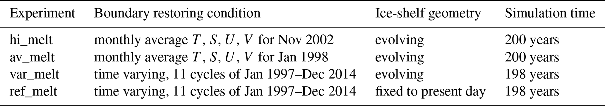
The second experiment corresponds to an average-melt scenario, henceforth referred to as av_melt, with average oceanographic conditions from January 1998 imposed at the open boundaries. The corresponding ocean state is characteristic for average-amplitude, high-prevalence melt rates (Fig. 2), with the exception of the Crosson and Dotson cavities, where conditions are biased towards lower-than-average melt rates. Similarly to the hi_melt experiment, the choice of January 1998 conditions was based on the histograms in Fig. 2, with melt rates that are characteristic for the January 1997–December 2014 period. Other choices of boundary conditions might have led to a comparable ocean state and melt rates but were not tested.
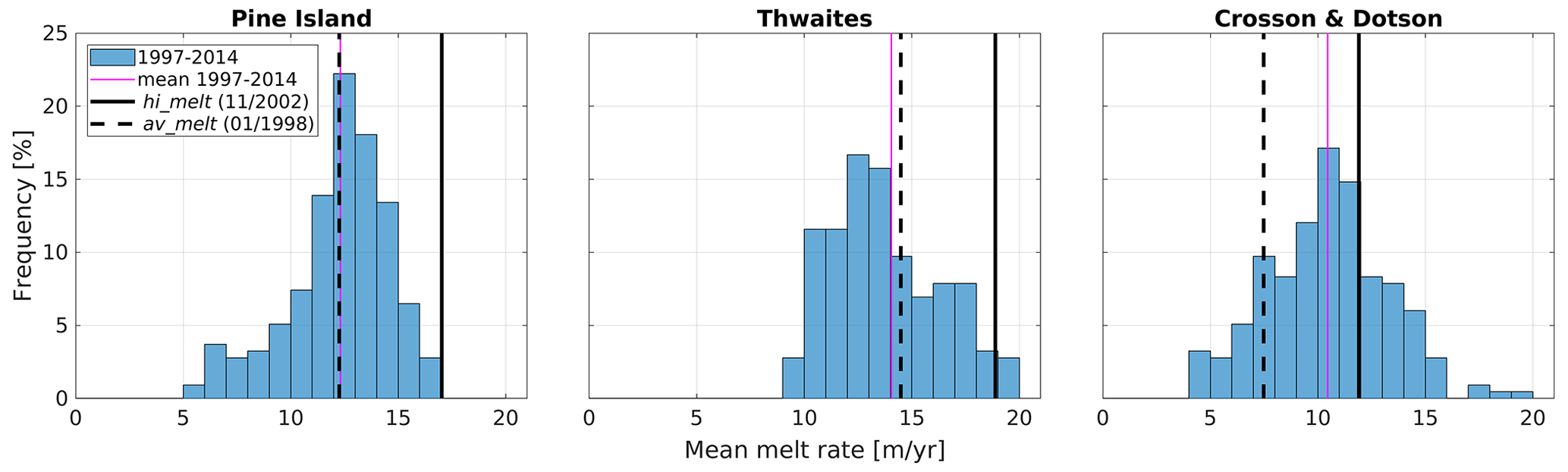
Figure 2Frequency distribution of monthly mean melt rates for each ice shelf, as simulated during the first cycle of the var_melt experiment, covering the January 1997 to December 2014 period. The magenta line indicates the mean melt rate over the entire simulation period. The solid and dashed lines indicate melt rates that correspond to the ocean forcing applied in the hi_melt and av_melt experiments, respectively.
For completeness, a low-melt scenario with a deep thermocline was considered, which resulted in a persistently positive mass balance of the ice shelves and a readvance of the grounding lines. Since this behaviour is unlikely to inform us about the future evolution of glaciers in the Amundsen basin, this scenario was not considered further.
In the second set of experiments, time-varying restoring conditions were applied at the MITgcm boundaries. The aim was not to carry out projections for different emissions scenarios but rather to disentangle geometrical feedbacks from the sensitivity of melt to natural variability in the ocean state. Monthly averaged ocean conditions between January 1997 and December 2014 from Kimura et al. (2017) were imposed at the MITgcm boundary and linearly interpolated onto the model time. The 1997–2014 restoring conditions were cyclically repeated 11 times for a total of 198 simulation years. The frequency distribution of melt rates during the first cycle is shown in Fig. 2. In addition to a coupled ice–ocean simulation with a dynamic ice-shelf geometry (referred to as var_melt), a reference stand-alone ocean simulation with fixed ice-shelf cavities was carried out (referred to as ref_melt). For both experiments, the variability in basal ablation was analysed within each 18-year forcing cycle, as well as between successive cycles.
Despite the idealized nature of the ocean forcing, experiments induce an ice-sheet response that is informative for sustained present-day ocean conditions (av_melt and var_melt) and future climate conditions dominated by warm periods (hi_melt). The key advancement of this work is the inclusion of ice–ocean feedbacks simulated by a 3D ocean model. As will be argued in Sect. 6, such feedbacks play an important role in the dynamical evolution of the Amundsen Sea glaciers, and results provide a first step towards more definitive climate change scenario-based projections of mass loss in response to ocean-induced ice-shelf thinning over the next decades to centuries.
In order to diagnose the feedbacks between changes in basal melt, imposed ocean boundary conditions, and cavity geometry, a number of cavity transfer coefficients are introduced. Each time-varying coefficient will be shown to play a distinctive role in linking the far-field ocean properties to the basal-melt rates, while their values depend, to greater or lesser extent, on the complex changes in cavity geometry. More precisely, spatially averaged basal-melt rates, denoted by m, can be expressed as a product of the time-dependent thermal transfer coefficient ϵT, the momentum transfer coefficient ϵU, the outer-cavity transfer coefficient μ, and the time-varying ocean thermal driving at the ice front T⋆IF as follows:
where m0 is a constant defined in Eq. (5). The expression in Eq. (1) can be derived from the fundamental relationships between basal melt and properties of the oceanic mixed layer directly beneath the ice shelf, as discussed below.
3.1 Basal-melt parameterization
Under the assumption that turbulent mixing of heat towards the ice–ocean interface is dominated by shear instabilities in the current, basal-melt rates can be parameterized as a function of the thermal driving in the mixed layer, denoted by T⋆, and the friction velocity relative to the ice base, denoted by U⋆ (Jenkins and Bombosch, 1995):
with
where Tf is the salinity-dependent freezing point at the depth of the ice base, and , where Ti is the temperature of the ice. Values , ΓT=0.02, , , and were used for the quadratic drag coefficient, turbulent heat exchange coefficient, enthalpy of the fusion of ice, specific heat capacity of ice, and specific heat capacity of water, respectively. In all MITgcm simulations, basal-melt rates were calculated using the parameterization in Eq. (2), with T and U calculated as a weighted average of cell properties adjacent to the ice–ocean interface, as described in Sect. 2.1.
3.2 Thermal transfer coefficient ϵT
Cells adjacent to the ice–ocean interface will be referred to as the mixed layer to indicate that any vertical shear and thermohaline gradients that might exist in a thin boundary layer adjacent to the ice base remain unresolved due to the 20 m vertical resolution of the ocean model. Properties of the mixed layer – and, hence, basal-melt rates – are controlled by the thermal driving of water masses that enter the cavity. In particular, the temperature of the mixed layer is modulated by mixing of the ambient water with meltwater at the local freezing temperature. As a result, the thermal driving of the mixed layer can be defined as a fraction of the average thermal driving of the inflow T⋆in:
with being a space- and time-dependent dimensionless coefficient (Jenkins et al., 2018), which will henceforth be referred to as the thermal transfer coefficient. Details of how T⋆in is calculated are provided in Sect. 3.4.
3.3 Momentum transfer coefficient ϵU
Based on inherent properties of the conservation of mass, momentum, heat, and salt within the mixed layer, it has been argued that the friction velocity U⋆ also scales approximately linearly with the thermal driving (Holland et al., 2008). Analogously to Eq. (6), a scaling coefficient, henceforth denoted by ϵU and referred to as momentum transfer coefficient, is introduced to express this relationship:
where ϵU has dimensions of . Combining Eqs. (2), (6), and (7) then leads to
which expresses local melt rates as a quadratic function of the thermal driving and two transfer coefficients, ϵT and ϵU, which link the far-field driving to properties of the mixed layer.
3.4 Basal melt in the deep interior cavity
To facilitate the analysis of temporal changes in melt rates, Eq. (8) can be spatially averaged. One viable choice is to calculate average basal-melt rates for each ice shelf and to define T⋆in as the average thermal driving of the inflow across the corresponding ice front. One shortcoming of this simple diagnostic, however, is the loss of information about changes in melt that occur over small areas of glaciological importance, in particular in the vicinity of the grounding line. Since the steepest slopes of ice-shelf draft in the Amundsen Sea are typically found near the grounding line, ice-shelf-wide averages are dominated by melt rates in the relatively extensive, shallow areas above the thermocline. Since the focus of this study is on geometrical changes and basal-melt feedbacks in the deep interior of the cavities, a more appropriate diagnostic will be introduced below.

Figure 3(a) Plan view and (b) section along the dashed line in (a) of the Pine Island Ice Shelf, used to illustrate the concepts of the outer cavity and deep interior, which correspond to regions of the ice-shelf cavity with draft above and below −400 m, respectively. Key locations referred to in the main text are numbered 1–3: (1) section at the ice front where thermal driving of the inflow below −400 m (T⋆IF) is calculated, (2) section at the −400 m ice-shelf draft contour where thermal driving of the inflow into the deep cavity is calculated (T⋆DI), and (3) the oceanic mixed layer in the deep interior where the thermal deficiency (T⋆) and boundary current (U⋆) that determine the melt rates are calculated.
First, all cavities are divided into an outer region and a deep interior, as illustrated for the Pine Island Ice Shelf cavity in Fig. 3. The deep interior is defined as the part of the cavity with ice draft below −400 m. This bound approximates the shallowest depth at which mCDW is currently found on the Amundsen continental shelf (Dutrieux et al., 2014; Jenkins et al., 2018), and the deep interior can be thought of as ice-shelf regions that are directly exposed to (a modified form of) the warmest waters. Secondly, T⋆in is defined as the average thermal driving of the inflow across a vertical section along the −400 m ice draft contour, henceforth denoted by T⋆DI, where DI refers to deep interior. A schematic representation of T⋆DI is shown in Fig. 3 and is calculated as follows:
with being the horizontal length of the section; b and B being the ice draft and seafloor depth, respectively; being the water column thickness; being where the freezing temperature Tf is calculated at a given depth z; and θ being a Heaviside step function which is 0 or 1 for a negative or positive (i.e. outflowing or inflowing) normal velocity Un. Finally, the time evolution of average basal-melt rates in the deep interior can be expressed as a function of T⋆DI using Eqs. (2), (6), and (7):
In the above derivation, spatial gradients of heat diffusion into the ice were ignored, and a constant °C was assumed, such that K−1. Although spatial variations in Tf were accounted for in the calculation of basal melt in MITgcm, corrections are small and will be ignored for the purpose of this analysis. Notations and were introduced to represent coefficients averaged over the deep interior of each ice shelf, and was used to denote the area of the ice shelf with draft below −400 m. It can be shown that the covariance term is typically 1 order of magnitude smaller than the first term on the right-hand side and will be omitted from subsequent analysis.
3.5 Outer-cavity transfer coefficient μ
Under certain conditions, such as simulations of idealized cavity geometries with a flat bathymetry, properties of the inflow at the ice front propagate into the deep cavity without significant modification. As a result, T⋆DI is approximately equal to the thermal driving of the inflow at the ice front, henceforth denoted by T⋆IF and schematically represented in Fig. 3. For realistic cavities with complex geometry and ocean dynamics, however, the ratio between T⋆DI and T⋆IF can be significantly different from 1. Indeed, even though the outer cavities in the proximity of the ice front are flooded with mCDW, mixing of the mCDW with subglacial meltwater and/or topographic blocking can prevent the inflowing water from reaching the deep cavities unmodified. As a result, the ocean properties that drive the onset of subglacial melt plumes in the vicinity of the grounding line are not generally identical to properties of the inflow at the ice front. In order to characterize the relationship between properties of the inflow at the ice front and the thermal driving in the deep interior, the dimensionless, time-dependent outer-cavity transfer coefficient μ is introduced:
where T⋆IF is calculated as follows:
with width and . The coefficient μ provides an aggregated measure for the impact of outer-cavity ocean processes, including mixing and topographic steering, on the water properties that feed the buoyant meltwater plumes. The offset Δt in Eq. (11) accounts for the time lag between water flowing into the cavity at the ice front and reaching the deep interior, which is a measure of the cavity residence time. For a horizontal length scale of 100 km, which is characteristic for the Amundsen Sea ice shelves, and an average barotropic circulation at the ice front between 0.01 and 0.015 m s−1, the residence time is on the order of a few months. Since the far-field ocean conditions vary predominantly at interannual to decadal timescales, changes in the inflow evolve slowly compared to the cavity residence time, and Δt can be set to zero for a good approximation.
Only currents below −400 m are considered in the calculation of T⋆IF; this is for several reasons. Firstly, water masses that access the cavity at depth form the most important source of basal-meltwater production in the deep interior. Secondly, the cavity inflow above −400 m predominantly alters the mixed-layer properties and melt rates in the outer cavity. Although changes in the ice-shelf draft at the ice front caused significant variations in the shallow currents in some of the Úa-MITgcm simulations, they have little impact on the melt rates in the deep interior and will not be analysed here. Finally, as pointed out in Sect. 2, the model does not simulate surface processes in the open ocean, such as wind stress or heat and salt fluxes. Properties of the upper water column and deeper waters in areas with convective mixing are therefore not reliably represented. Several sensitivity tests (not shown here) indicate that results presented in subsequent sections are not critically dependent on the choice of the cut-off depth, and no notable differences were found if either −300 or −500 m was used to define T⋆IF instead.
3.6 Summary and application to MITgcm
Equations (10) and (11) can be combined to express the average melt of the deep interior cavity as a function of the thermal and momentum transfer coefficients ϵT and ϵU, the outer-cavity transfer coefficient μ, and the average thermal driving of the inflow at the ice front T⋆IF, as expressed in Eq. (1). To simplify the notation, the subscript DI and overlines have been dropped from , , and .
Variations in average thermal driving of the inflow at the ice front (T⋆IF) are strongly controlled by open-ocean dynamics and climate drivers, whereas characterize the large-scale cavity dynamics, which is expected to depend on the cavity geometry. The relative importance of T⋆IF and the transfer coefficients in controlling the temporal evolution of the melt rates as the cavity geometry evolves will be assessed in Sect. 4. To enable easy comparison between the different contributions, all quantities will be scaled by their respective values at t=0:
where , , and so on.
To calculate the quantities in Eq. (13) or, equivalently, Eqs. (10) and (11) from model output requires a discrete version of the equations. In MITgcm, all variables in Eq. (10), including m, U⋆, and T⋆, are defined at cell centres of the Arakawa C grid, and spatial integrals directly translate into discrete sums. The calculation of T⋆DI and T⋆IF in Eq. (11) requires the evaluation of line integrals along the −400 m ice draft contours and ice fronts, respectively. Draft contours were calculated from the discrete MITgcm geometry, leading to a connected sequence of line segments with nodes that coincide with MITgcm nodes or the midpoint between MITgcm nodes. Ocean state variables and geometric variables were linearly interpolated to the midpoint of each line segment; velocities were subsequently projected to obtain the flow perpendicular to each segment. The contour integral was then replaced by a sum over all line segments, and quantities were evaluated at the centre of each segment. For the calculation of T⋆IF at the ice front, a similar procedure was followed, but contour nodes were taken directly from the Úa mesh. Further details on how each transfer coefficient was calculated from raw MITgcm output can be found on GitHub. A link to the code has been provided in the “Code and data availability” statement at the end of the paper.
4.1 Evolution of melt rates and cavity geometry
A logical first step in the diagnosis of geometry–melt feedbacks in the deep interior of the Amundsen Sea cavities is to simulate the response of the coupled ice–ocean system for suppressed temporal variability of the inflow at the ice front; i.e. . In doing so, the time dependency of normalized basal-melt rates ( in Eq. 13) can be attributed solely to changes in the transfer coefficients, which capture changes in the cavity geometry, and any contamination from far-field ocean variability is eliminated. The experiments hi_melt and av_melt, described in Sect. 2.2, aim to achieve this by imposing time-invariant restoring conditions at the MITgcm boundaries for 200 years.
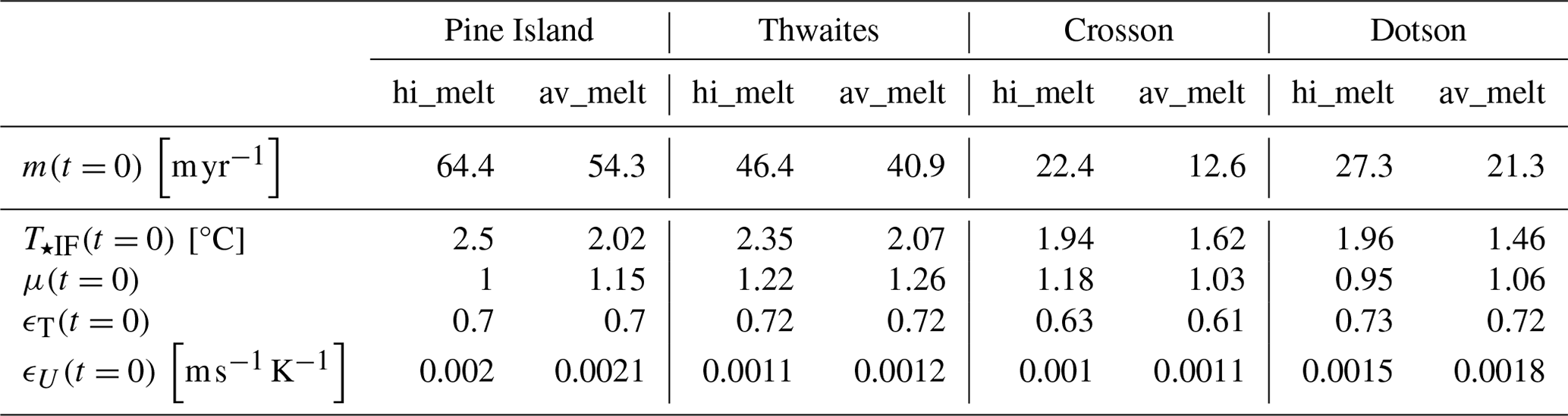
At the beginning of the hi_melt experiment, average basal-melt rates in the deep interior range from 22.4 m yr−1 (Crosson) to 64.4 m yr−1 (Pine Island), as listed in Table 2. Corresponding melt rates for the av_melt experiment are between 12.6 and 54.3 m yr−1. In both scenarios, pervasive thinning of all ice shelves causes significant inland migration of the grounding lines, as shown in Fig. 4 for the hi_melt experiment and Fig. S1 in the Supplement for the av_melt experiment. The strongest retreat is concentrated along the central trunk of Pine Island Glacier; in the Eastern Thwaites region; and at the Pope, Smith, and Kohler East glaciers, which flow into the Crosson Ice Shelf.

Figure 4Change in water column thickness between years 0 and 200 of the hi_melt experiment. The Úa-MITgcm grounding lines for both years are shown in black and magenta, respectively. For comparison, InSAR-derived grounding-line locations between 2011 and 2017 (Rignot et al., 2016; Milillo et al., 2019, 2022) are shown in orange. Background colours and contours represent the bed topography (Morlighem et al., 2020). Dashed black lines in panels (a) and (c) correspond to the location of the thermohaline sections in Fig. S2. The black star in panel (c) indicates the location of a bathymetric sill, discussed in Sect. 4.3.
Table 2Average melt rates (m), thermal driving of the inflow across the ice front (T⋆IF), and transfer coefficients (μ, ϵT, ϵU) at time 0 for the deep interior cavities, defined as areas of the ice shelf with draft below −400 m (Fig. 3). Note that, in agreement with Eq. (10), .
Concomitantly with changes in the cavity geometry, average melt rates in the deep interior respond to geometrical changes in diverse ways, as can be seen from the top row in Fig. 5. For the Crosson and Pine Island ice shelves, average melt rates in the deep interior increase by as much as 75 % and 35 %, respectively. Average melt rates for the Dotson Ice Shelf decrease by up to 75 %, whereas little to no changes occur for the Thwaites Ice Shelf. Whilst results for the hi_melt and av_melt simulations look broadly similar, the response of the latter is delayed due to the colder ocean thermal driving and slower evolution of the cavity geometries.
In the next four subsections, the physical processes that cause the varied response of basal melt to changes in ice-shelf geometry are explored. In particular, the evolution of the thermal driving at the ice front () and of the three transfer coefficients (, , ) is analysed, allowing us to draw general conclusions about the physical processes that control melt–geometry feedbacks independently of the specific geometric characteristics of each ice shelf. As will be shown in Sect. 4.5, the momentum transfer coefficient dominates the melt evolution, and a more in-depth analysis of the underlying dynamical causes is provided for each ice shelf.
4.2 Limited change in thermal driving at the ice front
Due to the two-way coupling between ice flux divergence and basal melt, a rich pattern of ice-shelf thickness change develops, and this evolves at a range of spatial and temporal scales. On average, the outer cavities in the hi_melt experiment expand vertically by 10 to 15 m per decade or between 200 and 300 m over the 200-year duration of the simulation, as shown in Fig. 4. This is consistent with present-day rates of ice-shelf thinning (Paolo et al., 2015; Adusumilli et al., 2018). The evolving water column thickness and variable freshwater input at the ice–ocean interface are coupled to changes in ocean currents and stratification in the cavities. These feedbacks can lead to significant variability in thermal driving of the inflow at the ice front despite the time-invariant restoring of ocean properties at the open boundaries of the domain and despite the absence of open-ocean surface fluxes. At the start of the hi_melt simulation, the average thermal driving of the deep inflow across the ice front () ranges from 2.5 and 2.35 °C for the Pine Island and Thwaites ice shelves to 1.94 and 1.96 °C for the Crosson and Dotson ice shelves (see Table 2). Values for the av_melt experiment are typically 0.3–0.5 °C lower.

Figure 5(a, b) Time series of average basal-melt rates in the deep interior cavities for the hi_melt and av_melt experiments, normalized by values at time = 0. (c, d) Square of the normalized thermal driving at the ice front, as defined in Eq. (12). (e–j) Time series of the normalized transfer coefficients , , and , which link the thermal driving at the ice front to melt rates in the deep interior according to Eq. (13). In all panels, thin lines correspond to monthly average values, whilst overlaying thick lines correspond to a 5-year moving average. The dashed vertical line at time t=0 indicates the beginning of the hi_melt and av_melt experiments. Values at negative times correspond to an 18-year hindcast simulation with 1997–2014 ocean forcing, as described in Appendix A.
To diagnose changes in the thermal driving of the cavity inflow and their impact on melt rates according to Eq. (13), a time series of is depicted in the second row of Fig. 5. All cavities experience notable variability up to 25 % at a range of timescales. High-frequency fluctuations at monthly timescales are predominantly caused by eddy activity at the ice front, which occurs irrespective of the changes in cavity geometry, as is apparent from identical simulations but with a fixed cavity geometry (not shown). At longer – decadal to century – timescales, trends in are small, except for a 20 % and 10 % increase for the Thwaites and Crosson ice shelves in the hi_melt experiment and a 25 %–30 % reduction for the Pine Island Ice Shelf in the av_melt experiment. The long-term trends are a consequence of complex changes in cavity geometry and are difficult to attribute to individual processes. For example, the decrease in thermal driving of the Pine Island Ice Shelf coincides with a westward shift of the inflow pathways across the ice front and vertical contraction of the mCDW core in conjunction with a reduced cyclonic re-circulation in the upper water column of the outer cavity, which adjusts to migrating channels in the underside of the ice shelf.
Overall, the connection between variability in T⋆IF and melt rates in the deep interior in the hi_melt and av_melt experiments is weak. Indeed, if the time-varying factor in Eq. (13) is replaced by its (constant) value at t=0, the root mean square error (RMSE) between the resulting time series and falls between 0.06 and 0.24 (see Fig. 6), which translates into relative errors in average melt of less than 15 %. The only exception is Pine Island Glacier in the av_melt experiment, with RMSE = 0.34, which equates to a geometry-driven suppression of basal melt of 20 %–25 %. Due to the overall small impact of changes in T⋆IF on the melt rates in the deep interior, a detailed analysis of the processes that influence T⋆IF is not pursued here.

Figure 6Root mean square error (RMSE) between and the corresponding time series where a factor is replaced by its constant value at t=0: , where ℱ corresponds to T⋆IF, μ, ϵT, or ϵU. RMSE values provide an indication of how much of the temporal variability in can be attributed to each factor. Further details are provided in Sect. 4 of the main text.
4.3 Geometrically constrained transport of water masses from the ice front to the interior cavity
Thermohaline properties of the cavity inflow do not invariably propagate into the deep interior. An aggregated measure for how outer-cavity processes can dampen or amplify changes in T⋆IF is provided by the outer-cavity transfer coefficient μ, defined in Eq. (11). At time t=0, values of μ are between 1 and 1.18 (Table 2), which implies that, on average, water masses that reach the deep cavity below −400 m have an equal or slightly higher thermal driving compared to water masses that cross the ice front. The amplification of thermal driving can occur through the complex interplay between ocean dynamics and topography, resulting in the blocking of water masses with lower thermal driving, which are typically found at shallower depths.
With time, however, dynamics of the coupled ice–ocean system cause μ to evolve in non-trivial ways. A time series of , which is the quantity of relevance for the calculation of the normalized melt rates in Eq. (13), is depicted in the third row of Fig. 5. Values higher (lower) than 1 correspond to an increased (decreased) connectivity between the ice front and deep interior compared to at the start of the simulations. Two key observations can be made.
Firstly, in both forcing scenarios, the Dotson Ice Shelf experiences a strong amplification of thermal driving in the deep interior as the cavity geometry evolves. Although the grounding line does not migrate by more than 2 km (Figs. 4 and S1) and shoals due to its retreat up a steep prograde bed slope (see Fig. S2 for a vertical section of the black line in Fig. 4c), the ice base rises by up to 300 m in places, which leads to a 2-fold increase in water column thickness. As a result, the gap between the ice base and a bathymetric sill at the location indicated by the star in Fig. 4c is increased, which enables more efficient transport of mCDW from the outer cavity into the deep interior (Fig. S2). This process, whereby shoaling of the ice draft enables warm waters to reach the grounding line, is similar to the mechanism that has been suggested to control the flow of mCDW towards the grounding line of Pine Island Glacier as it retreated from a bathymetric sill in the 1940s (De Rydt et al., 2014; Smith et al., 2017).
The second observation concerns the existence of high-frequency, monthly variability in , which is particularly evident for the Dotson Ice Shelf. For all ice shelves, these short-term fluctuations are strongly anti-correlated with monthly changes in . The transfer coefficient μ therefore acts as a dampening factor for high-frequency variability in the cavity inflow. Consequently, melt rates in the deep interior, as shown in Fig. 5, are found to be relatively insensitive to short-term, eddy-driven fluctuations in the thermal driving at the ice front.
The overall impact of changes in the outer-cavity transfer coefficient on basal-melt rates in the deep interior can be assessed by replacing the time-varying factor in Eq. 13) with its value at t=0. The RMSE values between the resulting time series and are provided in Fig. 6 and fall between 0.08 and 0.25, which is equivalent to relative errors less than 10 %. The only exception is the Dotson Ice Shelf, where the increase in thermal driving of the deep inflow causes a 50 %–60 % increase in average basal melt when compared to conditions at the start of the simulations. However, it will be shown in Sect. 4.5 that, despite the increase in ambient ocean thermal driving, melt rates of the Dotson Ice Shelf still decrease overall due to a reduction in the friction velocity relative to the ice base (U⋆ in Eq. 2).
4.4 Thermal driving of the ice–ocean boundary layer and deep inflow are linearly related
The third coefficient to impact average basal-melt rates in the deep interior cavities is the thermal transfer coefficient ϵT, defined in Eq. (6) as the ratio between the thermal driving of the deep inflow (T⋆DI in Fig. 3) and the thermal driving of the mixed layer adjacent to the ice–ocean interface (T⋆ in Fig. 3). Values of ϵT at t=0 vary between 0.7 and 0.73 for the Pine Island, Thwaites, and Dotson ice shelves (Table 2) and are somewhat lower for the Crosson Ice Shelf (0.61–0.63). Due to the input of cold freshwater at the ice–ocean interface, the thermal driving of the mixed layer is strictly lower than that of the ambient ocean – or ϵT<1. It should also be noted that, for reasons that will be explored below, the value of ϵT is approximately independent of the forcing scenario.
In both simulations, the temporal variability of ϵT is less than ±25 % (Fig. 5), with the largest changes found for the Crosson and Dotson ice shelves. To understand the physical mechanisms that cause the increase or reduction in ϵT over time, it is informative to analyse the relative importance of and underlying reasons for variations in T⋆DI and T⋆. In Fig. S3, a time series of ϵT for the hi_melt experiment is compared to and . It follows that, for all ice shelves except the Dotson Ice Shelf, variations in ϵT are dominated by changes in the thermal driving of the mixed layer T⋆. This can be understood as follows: for a given thermal driving of the inflow, variations in T⋆ are strongly linked to changes in the gradient of the ice-shelf base, which controls the efficiency of turbulent entrainment of heat across the thermocline between the ambient water and mixed layer (Pedersen, 1980; Jenkins, 1991). Indeed, as shown in Fig. S3, changes in broadly track changes in the average gradient of the ice draft in the deep interior (∇b). The average basal gradient of the interior Crosson Ice Shelf cavity, for example, steepens from 0.034 to 0.054 during the 200-year hi_melt simulation. This coincides with a 28 % increase in T⋆, whilst T⋆DI remains relatively constant and approximately equal to the thermal driving at the ice front ( in Fig. 5e). As a result, ϵT increases from about 0.62 to 0.78.
Whilst values of ϵT are generally linked to the slope of the ice draft and hence the cavity geometry, for the Dotson Ice Shelf, changes in ϵT are dominated by the previously highlighted increase in the thermal driving of the inflow ( in Fig. 5e). During the first 50 years of the simulation, this coincides with a rise in ice draft and a flattening of the ice-base gradients, as can be seen from the thermohaline section in Fig. S2. In turn, this causes a concurrent reduction in the thermal driving of the mixed layer (Fig. S3). Both increased thermal driving of the inflow and reduced thermal driving of the mixed layer cause the 20 % reduction in ϵT, as observed in Fig. 5g.
Whilst the foregoing discussion was primarily focused on results from the hi_melt experiment, results from the av_melt experiment were found to be qualitatively similar but delayed in time, as suggested by Fig. 5h.
Despite a demonstrable link between changes in ice-shelf draft and ϵT, the relative impact of temporal variations in ϵT on basal-melt rates in the deep interior is small. When the time-varying factor in Eq. (13) is replaced by its (constant) value at t=0, the RMSE between the resulting time series and falls between 0.02 and 0.17 (see Fig. 6) or a relative error in average basal-melt rates of less than 10 %. The only exception is the Crosson Ice Shelf, with an RMSE = 0.27 or a relative error around 20 %.
4.5 Changes in cavity circulation dominate melt rate evolution
The fourth and final coefficient controlling average melt rates in the deep interior is the momentum transfer coefficient ϵU, which links the mixed-layer velocity to the thermal driving of the inflow (Eq. 7). At decadal timescales, changes in ϵU dictate the majority of variability in the melt rates, as is apparent from the strong similarities between and in Fig. 5. Since the temporal variability in thermal driving of the deep inflow is relatively small – the Dotson Ice Shelf being the only exception – changes in ϵU are dominated by variability in the mixed-layer friction velocity U⋆. This is demonstrated in Fig. S4, which shows a strong agreement between ϵU and , whereas the similarity to is much weaker.
Based on a general scaling analysis, Holland et al. (2008) argued that, for a given cavity geometry, U⋆ depends approximately linearly on the far-field thermal driving. Results from the hi_melt and av_melt experiments suggest that the linear scaling factor ϵU is strongly dependent on the geometry of the cavity. Whilst no studies have considered this dependency in detail, insights from 2D plume theory (Lazeroms et al., 2019) and numerical ocean simulations for simplified ice-shelf shapes (Holland et al., 2008) suggest that ϵU is a monotonically increasing function of the gradient of the ice base. However, analysis of the hi_melt and av_melt experiments does not support such a monotonically increasing relationship. Instead, the two quantities are found to be weakly anti-correlated (not shown), indicating that ϵU cannot be quantified in terms of the geometry of the ice base alone; furthermore, spatially averaged ice-shelf basal gradients only play a subsidiary role in controlling the friction velocity U⋆, at least for the complex geometries presented here.
To understand how U⋆ (and therefore ϵU and melt rates m) vary with changes in cavity geometry, it is informative to analyse the barotropic and overturning components of the cavity circulation. The time evolution of the barotropic stream function amplitude is shown in Fig. 7a–d. The stream function amplitude, which is defined as the difference between the maximum and minimum values of the barotropic stream function in the deep interior (delineated by the magenta lines in Fig. 7e–f), is a measure for the strength of the horizontal transport within the cavity. Figure 7a–d show that, over time, the strength of the horizontal circulation in the Pine Island and Dotson ice-shelf cavities increases and decreases, respectively. On the other hand, no significant changes in the barotropic flow are simulated beneath the Thwaites Ice Shelf, whereas the circulation in the Crosson Ice Shelf cavity first increases and is subsequently reduced. Figure 7a–d also show that variations in the barotropic stream function amplitude closely track changes in average basal-melt rates.

Figure 7(a–d) Average melt rates in the deep interior cavities (black lines, left y axis) are shown alongside the barotropic and overturning stream function amplitudes (red and green lines, right y axis; note the different limits). The latter are calculated from the meridional (Pine Island) and zonal (Thwaites, Crosson, Dotson) transport within the boxes outlined by dashed green lines in panel (f). (e, f) Barotropic stream function at years 0 and 200. Magenta lines delineate the boundaries of the deep interior cavities, i.e. areas with ice-shelf draft below −400 m. All plots are based on the hi_melt experiment.
Together with the variability in horizontal transport, changes in basal-meltwater production dominate the buoyancy-driven overturning circulation of the Amundsen cavities, as noted previously by Jourdain et al. (2017). For each cavity, a measure of the overturning strength was obtained from the meridional (Pine Island) or zonal (Thwaites, Crosson, Dotson) overturning stream function amplitude, calculated for the areas enclosed by the boxes with dashed lines in Fig. 7e. Time series of the overturning stream function amplitude in Fig. 7a–d indeed show temporal variability that is comparable to changes in the barotropic stream function amplitude and basal-melt rates. It is important to reiterate that, whilst gradients of the ice base do locally affect the buoyancy of the mixed layer and influence horizontal pressure gradients that determine the vertical shear, changes in the average basal gradient of the deep interior ice shelves (see Fig. S3) do not correlate with changes in the overturning amplitude or average melt rates.
The above results suggest that extensive geometrical changes, which unfold over multi-annual to decadal timescales, can induce persistent adjustments to the large-scale horizontal and overturning circulation within the cavity. This coincides with comparable changes in the mixed-layer friction velocity U⋆ and hence in the melt rates. To understand how changes in cavity geometry and circulation are connected, one should recall that the barotropic circulation is constrained by the conservation of barotropic potential vorticity or BPV (Patmore et al., 2019, or Bradley et al., 2022). This implies that, to leading order, the depth-averaged flow aligns with contours of constant , where f is the Coriolis parameter, which is approximately constant for the region of interest; ζ is the depth-averaged relative vorticity; and H is the spatially variable water column thickness. Over time, the temporally evolving water column thickness can induce significant changes in the spatial distribution of BPV and hence in the 3D structure of the circulation.
Whilst the discussion above was based on results from the hi_melt experiment, panel (j) in Fig. 5 shows that an equally significant relationship between ϵU (and hence U⋆) and melt rates exists for the av_melt experiment. The dominant impact of geometrically induced changes in the cavity circulation on the melt rates is therefore independent of the specific realization of far-field ocean forcing used in the hi_melt and av_melt experiments. The only key difference is the timescale at which those geometry–melt feedbacks unfold. Compared to the hi_melt experiment, the cavity geometries in the av_melt evolve more slowly due to the lower ocean thermal forcing, which causes an associated delay in the melt rate response.
Given the important links between changes in cavity geometry, circulation, and basal melt, a more detailed account of the feedbacks for individual ice shelves is provided below.
With regard to the Pine Island Ice Shelf, changes in cavity circulation result in a 75 % increase in ϵU during the first 60 years of the simulation (Fig. 5i), followed by relatively constant values of ϵU. This coincides with a 3-fold increase in and levelling off of the barotropic and overturning stream function amplitudes (Fig. 7a) and a 50 % increase in basal-melt rates.
The Pine Island Ice Shelf provides a clear example of how BPV and the depth-averaged cavity circulation co-evolve over time. During the first 60 years of the hi_melt simulation, BPV in the deep interior cavity becomes generally less negative due to an increase in water column thickness H, as shown in Fig. S5. At all times, no continuous contours of BPV exist that link the outer cavity to the deep interior, in part due to the existence of a prominent bathymetric sill that extends from north to south (left to right in the figure) around x=300 km (Jenkins et al., 2010). As a result, there are no direct pathways of barotropic flow between the outer cavity and deep interior that conserve BPV, and the cavity circulation is divided into two cyclonic gyres (one in the deep interior, one in the outer cavity) separated by an anticyclonic current on the seaward side of the sill. This current structure, which is illustrated by the barotropic stream function in Fig. 7e at year 0, was previously reported by Dutrieux et al. (2014) and Bradley et al. (2022). As the grounding-line retreats between years 0 and 60, the area with continuous contours of BPV landward of the sill doubles in size (the region indicated by the box with dashed lines in Fig. S5), which allows the cyclonic gyre to laterally expand. At the same time, the strength of the gyre increases from about 0.25 to 0.65 Sv, sustained by the almost 2-fold increase in meltwater production (and associated increase in buoyancy) in the cavity interior from 50 to 90 Gt yr−1. The expansion and strengthening of the gyre is illustrated by the barotropic stream function for year 200 in Fig. 7f. As the Pine Island grounding line retreats, the average gradient of the ice base does not significantly change (see Fig. S2, which represents a section of temperature and salinity along the dashed line in Fig. 4a). Instead, the increase in meltwater production is enabled and sustained by changes in the large-scale barotropic and overturning circulation within the deep interior.
For the Thwaites Ice Shelf, neither ϵU nor the barotropic or overturning circulation display any significant variability over the duration of the simulations (Fig. 7b). As a result, average basal-melt rates in the deep interior cavity remain approximately constant. This does not contradict results from Holland et al. (2023) as the simulations presented here do not include the same detailed retreat of the Western Thwaites Ice Tongue. Instead, at the start of the simulations, the Thwaites grounding line has already retreated past the pinning point that was highlighted by Holland et al. (2023) as the main geometric control on basal-melt rates of the Thwaites Ice Tongue. The lack of any strong geometrical feedbacks can be explained by the shallow ( m) and relatively featureless bedrock topography over which the Eastern Thwaites grounding line retreats (Fig. 4). A narrow band of relatively low melt rates (<50 m yr−1) tracks the moving grounding line (not shown) without significant modification to the geometrical configuration and current speed. This might change once the grounding line of the western Thwaites Glacier retreats inland from the subglacial ridge it is currently pinned on. However, this does not occur over the 200-year duration of the simulations presented here.
For the Crosson Ice Shelf, a sharp increase and decline in ϵU during the first 50 years (Fig. 5i) are followed by approximately constant values for the remainder of the simulation. This coincides with equivalent changes in the barotropic and overturning stream function amplitudes in Fig. 7c. The sharp increase in flow speed and the subsequent decline are linked to the ungrounding of several large ice rises downstream of the main grounding line of the Smith Glacier, indicated by the black box near the bottom of Fig. 7e. The removal of these topographic barriers causes a reorganization of the cavity circulation and melt rate distribution, which stabilizes after about 50 years, and the Smith Glacier continues its retreat into a deep, narrow trough without further significant changes to the current structure.
For the Dotson Ice Shelf, the gradual 4-fold decrease in ϵU (Fig. 5i) coincides with a 4-fold reduction in the barotropic and overturning stream function amplitude, as shown in Fig. 7d (correlation coefficient 0.97). The slow-down of the circulation is largely explained by the loss of buoyancy as the grounding line retreats up a prograde bed slope, and the ice draft rises above the thermocline in most places. This process is illustrated in the top row of Fig. S2.
So far, geometrically driven changes in basal melt have been discussed in the context of suppressed variability of the far-field ocean. In reality, interannual to multi-decadal shifts in ocean conditions, linked to internal climate variability and anthropogenic trends in the atmosphere, are understood to be important regulators of ice-shelf melt in the Amundsen Sea. Aided by repeat measurements of ocean properties on the continental shelf, significant progress has been made in understanding the links between natural climate variability, including tropical ENSO activity, and decadal variations in basal melt (Jenkins et al., 2016, and references therein; Silvano et al., 2022). On the other hand, the impact of past and future anthropogenic climate change on ice-shelf melt in the Amundsen Sea has only recently started to be addressed in global (Timmermann and Hellmer, 2013; Naughten et al., 2018; Siahaan et al., 2022) and regional (Naughten et al., 2022; Jourdain et al., 2022) ocean model set-ups with thermodynamically active ice-shelf cavities. Of the studies above, only Siahaan et al. (2022) included a dynamically evolving ice sheet. However, the 1° resolution of their global ocean configuration was too coarse to reliably capture the spatial distribution of melt rates beneath the small Amundsen Sea ice shelves. In this section, a step is taken towards addressing this shortcoming. In particular, the combined impact of naturally occurring (present-day) ocean variability in the Amundsen Sea Embayment and geometrically driven changes in melt rates is considered at a much higher horizontal resolution (1.3 km) than previously achieved. Uncertain anthropogenic trends in regional ocean conditions are not included here but are the subject of a forthcoming study.
To compare geometrically driven changes in melt to changes caused by interannual to decadal variations in far-field ocean conditions, two numerical experiments were conducted, ref_melt and var_melt, as described in Sect. 2.2. In the ref_melt experiment, the ocean state was restored at the eastern and northern open boundaries to monthly average conditions over an 18-year period (January 1997–December 2014), repeated 11 times, whilst the cavity geometry was kept fixed to its present-day configuration (see Appendix A for details about the geometry). A 5-year moving average of mean melt rates in the deep interior cavities, shown in Fig. 8, displays 11 near-identical cycles with interannual variability ranging from 20 % (Thwaites) to 50 %–60 % (Pine Island and Dotson) and 80 % (Crosson). The results for fixed ice-shelf cavities are plotted alongside results from the var_melt experiment, which imposes the same oceanographic restoring conditions but additionally includes evolving cavity geometries. Three broad conclusions can be drawn.

Figure 8The 5-year moving average of melt rates in the deep interior cavities for the ref_melt experiment (cyclic restoration of 1997–2014 ocean boundary conditions with static cavities), the var_melt experiment (cyclic restoring conditions with evolving cavities), and the av_melt experiment (constant restoring conditions with evolving cavities).
-
The basal-melt variability in the var_melt experiment consists of interannual changes superimposed onto a (multi-)decadal trend. The latter is absent from the ref_melt experiment but closely resembles the long-term variability in the av_melt experiment (red line in Fig. 8), providing evidence for its geometrical origin. Results suggest that, whilst basal-melt variability is dominated by internal climate variability at decadal timescales, changes in cavity geometry can play a non-negligible role at longer timescales. In particular, it should be noted that the impact of geometrical feedbacks can cause both a long-term amplification of basal melt, as is the case for the Pine Island Ice Shelf, and a long-term suppression of basal melt, as is the case for the Dotson Ice Shelf.
-
Interannual changes caused by far-field ocean variability and multi-decadal trends caused by geometrical feedbacks are not independent. Indeed, the amplitude of interannual melt variability differs between individual 18-year cycles in the var_melt experiment, which indicates that the sensitivity of melt rates to (inter)annual changes in far-field ocean conditions depends on the cavity geometry. This is particularly evident for the Pine Island Ice Shelf, showing lower amplitude variations in years 75–115, compared to, e.g. years 125–200. Whilst average melt rates scale approximately quadratically with the thermal driving of the inflow within each 18-year cycle (not shown), the scaling factor does not remain constant between cycles. This is consistent with the results presented in Sect. 4, which highlighted the strong dependency of the scaling factor (μ2ϵTϵU in Eq. 1) on the cavity geometry.
-
For the Pine Island and Thwaites ice shelves, the envelope of melt variability in the var_melt experiment falls outside the range of variability in the ref_melt experiment, underlining the dominant impact of geometrical feedbacks on the melt rates. Over the 200-year duration of the experiments, the average difference between the var_melt and ref_melt melt time series is 22 m yr−1 or 58 % for the Pine Island Ice Shelf, −9.4 m yr−1 or −19 % for the Thwaites Ice Shelf, −2.3 m yr−1 or −8 % for the Crosson Ice Shelf, and −3.3 m yr−1 or −16 % for the Dotson Ice Shelf. In all cases except for the Pine Island Ice Shelf, simulations that ignore geometrical feedbacks overestimate future melt rates forced by present-day ocean conditions. It remains to be shown that this conclusion holds in simulations with realistic atmosphere–ocean interactions and for weaker ocean restoring conditions that allow complex feedbacks between meltwater production, sea ice production, and water mass properties on the continental shelf.
A prime objective of the preceding analysis was to identify potential feedbacks in the ice–ocean system, whereby grounding-line retreat triggers changes in ocean dynamics with lasting implications for the ice-shelf mass balance, independent of the far-field ocean conditions. Whilst the focus has been on the response of ocean-driven melt to changes in cavity geometry, the impact of geometrical feedbacks on the net mass balance of the ice shelves, including grounding-line fluxes, needs to be considered in order to assess their importance for the future dynamics of the Antarctic Ice Sheet.
In broad agreement with the observational record (Depoorter et al., 2013), ice shelves in the Úa-MITgcm 1997–2014 hindcast simulation (Appendix A) have a negative net mass balance between −40 and −10 Gt yr−1, as shown by the black line for negative times (grey-shaded area) in Fig. 9. The interannual variability in mass changes during the hindcast period arises predominantly from changes in ice-shelf basal melting (solid and dashed blue lines in Fig. 9) due to variations in the thermocline depth of the far-field ocean forcing. The corresponding variations in grounding-line discharge (red line) and ice front flux (orange line) during the hindcast period have a much lower amplitude.
It is prudent to recall that, in all simulations, the surface mass balance (SMB, green lines) was kept constant and equal to a 1979–2015 climatology (van Wessem et al., 2018). While this assumption might not be valid in century-scale projections, present-day surface accumulation only contributes a small fraction of the total ice-shelf mass balance in the region, and any impact of temporal variability on the net mass balance of the ice shelves will be disregarded. Furthermore, the ice front was fixed to its 1997 location, even though variations in ice-shelf extent and associated changes in buttressing have been shown to impact on the ice-shelf mass balance in recent years (Joughin et al., 2021; Bradley et al., 2022). Equally, changes in ice-shelf rheology, including rifting and fracturing, have been ignored despite their importance for ice-shelf and ice-sheet dynamics in the region (De Rydt et al., 2021; Surawy-Stepney et al., 2023).
The focus in the remainder of this section will be on results from the var_melt experiment. Through repeat forcing of present-day decadal variability in ocean conditions and the inclusion of evolving cavity geometries, results from this simulation capture the combined impact of decadal ocean variability and geometrical feedbacks on the net mass balance of the ice shelves. Similar results for the hi_melt experiment with fixed ocean boundary conditions are provided in Fig. S6 and will be discussed briefly at the end.
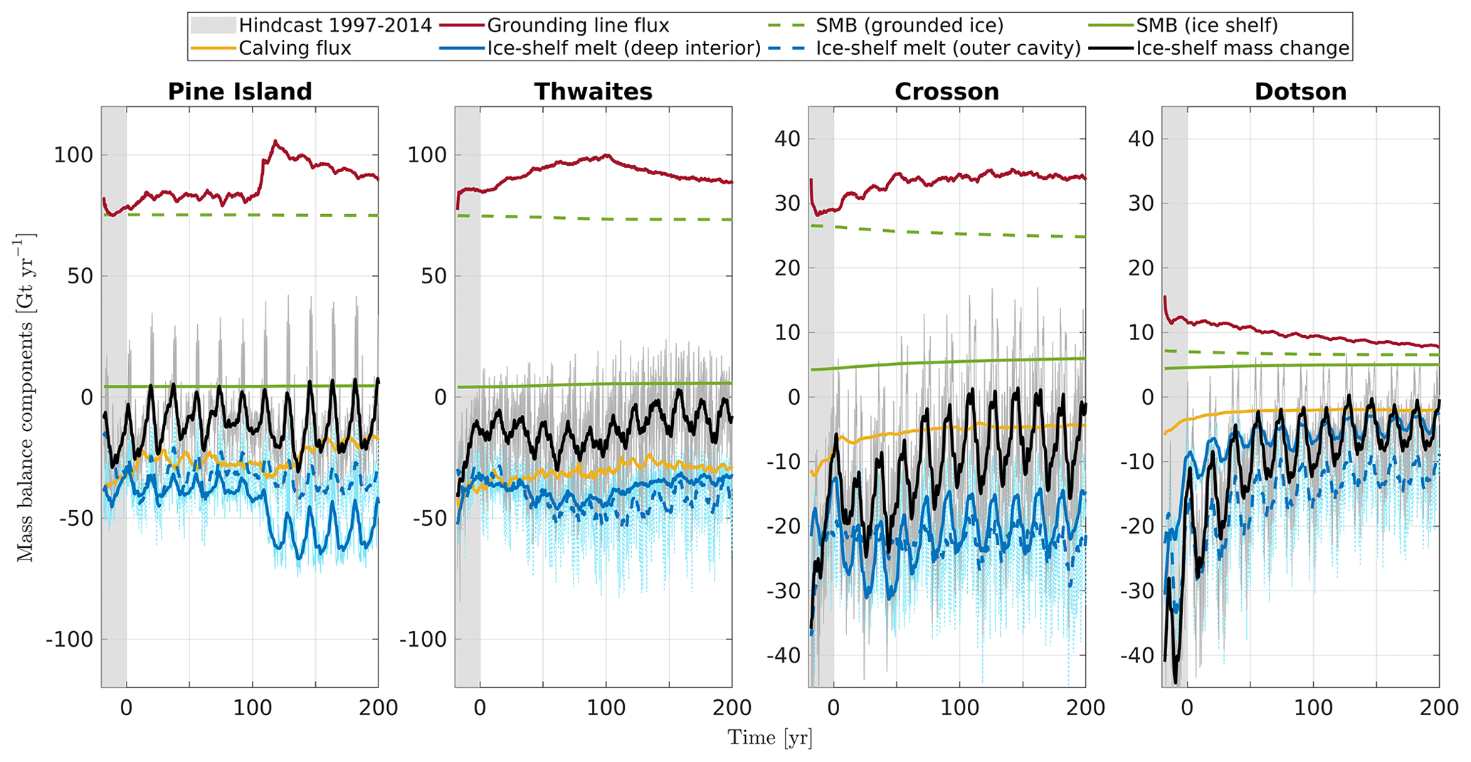
Figure 9Temporal evolution of integrated mass balance components in the hindcast experiment (grey-shaded area; see Appendix A for details) and the var_melt experiment (0 to 200 years; see Sect. 2.2 for details). Ice-shelf mass changes (black curve) are equal to the sum of the grounding-line flux (red curve), surface mass balance (SMB, solid green curve), calving flux (orange line), ice-shelf melt in the deep interior (solid blue line), and ice-shelf melt in the outer cavity (dashed blue line). For reference, the SMB of the grounded ice is represented by the dashed green line and is lower than the grounding-line flux, indicating net mass loss (or positive sea-level contribution) from each glacier basin.
Results in Fig. 9 show that, between years 0 and 200, the net mass balance of all ice shelves remains negative under the imposed ocean and atmospheric conditions. Only during intermittent episodes of 1 to 5 years does lower-than-average basal melting cause a positive net mass balance. Such episodes of positive net mass balance occur more frequently towards the end of the simulation, when ice-shelf mass changes tend toward less negative values for the Thwaites, Crosson, and Dotson ice shelves. Broadly speaking, fluctuations in basal mass loss, both in the deep interior and outer cavities (solid and dashed blue lines in Fig. 9, respectively) dominate the variability in the net mass balance of the ice shelves at decadal timescales. The amplitude of variations in grounding-line flux, surface mass balance, and ice front (or calving) fluxes is significantly lower. At longer timescales, however, significant shifts in grounding-line flux occur. One notable example is the rapid 40 % increase in the grounding-line discharge of the Pine Island Glacier between years 100 and 120. For other ice shelves, changes in mass influx across the grounding line evolve more gradually, at least in the var_melt experiment, with a 25 % (0.2 Gt yr−2) increase over 100 years for the Thwaites Ice Shelf, a 15 % (0.1 Gt yr−2) increase over 50 years for the Crosson Ice Shelf, and a gradual 30 % (0.02 Gt yr−2) decline over 200 years for the Dotson Ice Shelf.
Without a compensating response of other components of the ice-shelf mass balance, the increase in grounding-line flux for the Pine Island, Thwaites, and Crosson ice shelves would imply a smaller negative or even positive net mass balance. For the Pine Island Ice Shelf in particular, the 40 % (or 30 Gt yr−1) increase in grounding-line flux would lead to a persistently positive net mass balance, causing the ice shelf to thicken and enabling the glacier to readvance. Instead, the abrupt change in grounding-line flux is largely compensated for by a shift in basal mass loss in the deep interior cavity, which enables the sustained thinning of the ice shelf and associated retreat of the grounding line. Similar findings apply to the other ice shelves: multi-decadal trends in grounding-line flux are largely compensated for by shifts in basal mass loss with similar magnitude but opposite sign. While changes in ice-front discharge occur too, they manifest themselves at longer timescales, and their general decline tends to shift the net ice-shelf mass balance towards more positive values rather than counteract the changes in grounding-line flux.
The finding that melt rates play an important role in sustaining the negative mass balance of the ice shelves despite significant changes in grounding-line flux is not new. However, the physical mechanisms by which they do so have not previously been studied in detail. In particular, mechanisms that enable sustained adjustments in basal mass loss that occur independently of the external forcing have not been explored. In this study, the close interaction between changes in cavity geometry, ocean circulation, and basal melt has been identified as a candidate for such a mechanism. For example, based on the analysis in preceding sections, the 60 % increase in meltwater flux in the deep interior of the Pine Island Ice Shelf cavity between 100 and 120 years is enabled by a strong adjustment of the barotropic flow in response to changes in the cavity geometry. At the point where no further geometry-driven changes in circulation and melt rate occur, an increasing mass flux across the grounding line cannot be accommodated without causing a less negative or positive net ice-shelf mass balance. As a result, ice-shelf thinning and grounding-line retreat are either slowed down or prevented. Results from the var_melt experiment indicate that this is more generally true: peaks in grounding-line discharge coincide with a maximum in ice-shelf basal mass loss for all ice shelves, except for the Dotson Ice Shelf. The evolution of the latter is somewhat different as it experiences a gradual decline in grounding-line flux despite a persistent negative net mass balance of the ice shelf. Changes in grounding-line flux are small, however, compared to the strongly negative trend in basal mass loss, which drives the net mass balance towards zero. The 75 % reduction in basal-melt rates is again linked to changes in cavity geometry, as argued in Sect. 4, and drives the system towards a new equilibrium state, with the grounding line of the tributary Kohler West Glacier (Fig. 4) located on a prominent bathymetric sill (Fig. S2).
Broadly similar conclusions can be drawn from the hi_melt experiment (Fig. S6) and the av_melt experiment (not shown). For both simulations, despite the absence of temporal variability in ocean forcing, sudden or gradual increases in grounding-line discharge into the Pine Island, Thwaites, and Crosson ice shelves are largely compensated for by an increase in ice-shelf basal mass loss. Based on the analysis in preceding sections, such changes in basal melt can be linked to an adjustment of the cavity circulation in response to changes in the cavity geometry. Melt–geometry feedbacks therefore enable a sustained negative net mass balance of the ice shelves and promote ongoing retreat of the grounding line independently of the far-field oceanographic conditions. As a final comment it is worth noting that, whilst this mechanism operates under current glaciological conditions, dynamical instabilities such as the marine ice sheet instability (e.g. Weertman, 1974) can cause sustained retreat of the grounding line independently of the amount of basal mass loss. However, no evidence for such a mechanism was detected here.
Numerical simulations with a high-resolution coupled ice–ocean model were used to quantify the connection and feedbacks between changes in cavity geometry and basal melting of ice shelves in the Amundsen Sea Embayment, West Antarctica. Under a range of present-day ocean conditions, sustained thinning of the Pine Island, Thwaites, Crosson, and Dotson ice shelves was shown to cause pervasive retreat of the grounding lines by up to 50 km over a 200-year period. For each ice shelf, extensive changes in cavity geometry led to persistent dynamical adjustments of the ocean circulation and to opposing changes in basal melt near the grounding lines. In particular, a significant correlation was found between the geometrical amplification (e.g. Pine Island) or suppression (e.g. Dotson) of the cavity circulation and the up-to 75 % increase (Pine Island) or 75 % decrease (Dotson) in average basal-melt rate. The main conclusions and implications are summarized as follows.
At multi-annual to decadal timescales, feedbacks between ice-shelf geometry and basal-melt rates are dominated by changes in the friction velocity at the ice base (U⋆). A much smaller proportion of the variability is explained by geometrically induced changes in thermal driving at the ice base. Simulated changes in U⋆ are dynamically linked to variability in the barotropic and overturning circulation, whilst no significant relationship was found between changes in melt and simple geometric characteristics of the ice shelf, such as the depth or gradient of the ice base. The changes in melt are therefore controlled by complex adjustments of the ocean dynamics to the 3D evolution of the cavity geometry. This has important implications for commonly used parameterizations of basal melt, which are typically calibrated for present-day ice-shelf geometries and depend on (local) gradients and/or the depth of the ice base alone. Since these parameterizations do not account for the effects of changes in cavity circulation, their application to geometrically complex settings over timescales that allow significant adjustments of the water column thickness should be carefully tested. The results in this study suggest that the timescales over which geometrical feedbacks dominate the melt variability can be as short as several decades.
The physical processes that control melt-geometry feedbacks operate irrespective of the far-field ocean forcing, although the latter has a strong impact on the timescales over which the feedbacks unfold. While results suggest that internal climate variability dominates the basal-melt variability in the Amundsen Sea over multi-annual timescales, rapid and extensive adjustments of the cavity circulation over decadal timescales can lead to sustained changes in melt that outweigh variations due to natural variability in far-field ocean properties. Importantly, simulations with a static cavity geometry can lead to a systematic positive or negative bias in melt rate projections by up to 75 % compared to simulations that include a dynamic ice sheet. Melt estimates for static, present-day cavity geometries should therefore be treated with caution. Moreover, geometrically-induced trends in melt rates should be considered alongside anthropogenic climate trends as they could greatly amplify or reduce the impact of climate change on the ice-shelf mass balance.
While it is well known that rates of grounded ice loss are regulated by the amount of buttressing provided by the adjacent ice shelves, results from this study suggest that melt–geometry feedbacks can play an important role in controlling the dynamical connection between grounded and floating ice. For all glaciers except the Kohler West Glacier, a sustained increase in grounding-line discharge by up to 30 % is simulated, while changes in calving flux and total ice-shelf area are relatively small. Yet, the net mass balance of the ice shelves remains negative. In all cases, the increased discharge across the grounding line is offset by a geometrically induced increase in average basal melting, allowing further ice-shelf thinning, grounding-line retreat, and mass loss. While the glacier mechanics of this process have been well understood in principle, results in this study have highlighted the important role of ocean dynamics in controlling basal-melt rates.
The Úa-MITgcm simulations presented in the main part of the paper were preceded by a spin-up and hindcast simulation, as indicated by the flow diagram in Fig. A1. Given the abundant evidence that ice-sheet models, either in stand-alone mode (Seroussi et al., 2019) or coupled to an ocean model (Goldberg and Holland, 2022), retain information about their initial state that can dominate the future evolution of the ice sheet, along with the fact that diverse approaches to (coupled) model initialization are used in the literature, a detailed account of the Úa, MITgcm, and Úa-MITgcm initialization procedures is provided in Sect. A1. A basic validation of the coupled configuration, based on a 1997–2014 hindcast simulation, is provided in Sect. A2.

Figure A1Flow chart showing the different steps in the initialization, spin-up, and validation of the coupled ice–ocean model Úa-MITgcm. Details about the initialization and spin-up of the stand-alone Úa and MITgcm configurations are provided in Sect. A1. Results from a Úa-MITgcm hindcast simulation between 1997 and 2014 are provided in Sect. A1. Results from the 200-year perturbation experiments (hi_melt, av_melt, and var_melt) are presented and discussed in the main part of the text.
A1 Initialization and spin-up
As a first step in the initialization of the coupled Úa-MITgcm configuration, the ice flow model Úa was calibrated using an inverse method, first introduced by Macayeal (1992) and now frequently used in ice-sheet modelling (e.g. De Rydt et al., 2021; Barnes et al., 2021). The inverse step resulted in optimal estimates of the spatially varying rate factor (A) in Glen's law and the slipperiness (C) in the basal-sliding law for a given ice-sheet geometry and surface velocity measurements (uobs) with corresponding errors (εu). Values for the A and C fields were obtained as a solution to the minimization problem , where the cost function J was defined as the sum of the misfit terms for the surface velocities and ice thickness changes and a Tikhonov regularization term, , with
where is the total area of the domain, and pi and , with , are shorthand notation for p1=A, p2=C, and their respective priors and . Values of the pre-multipliers , , and were chosen based on a common L-curve approach (De Rydt et al., 2021). The velocity observations (uobs) and corresponding errors (εu) in the first misfit term were taken from the ERS-1/2 InSAR tandem mission in late 1995–early 1996 (Rignot et al., 2004). Ice thickness changes were set to zero everywhere (), with errors of and for grounded and floating ice, respectively. The ice-sheet geometry was assembled from a combination of Bedmachine Antarctica v2 data for the bed geometry (Morlighem et al., 2020) and the Icesat-corrected surface DEM from the ERS-1/2 mission with an effective timestamp in 2004 (Bamber and Griggs, 2009). Nominal ice densities (917 kg m−3) were corrected using a climatology of the firn density and thickness distribution from the RACMO2.3 data set between 1979 and 2013 (van Wessem et al., 2018). The inversion for A and C was stopped after 1000 iterations, with a mean and standard deviation in terms of the misfit between modelled and observed surface speeds of 12 and 61 m yr−1, respectively.
Following the inversion step, the transient evolution of the ice sheet can be contaminated by unrealistic short-wavelength (<10 km), large-amplitude (>10 m yr−1) adjustments that dominate changes in ice thickness during the first few years of the simulation. These adjustments arise from a force imbalance due to inconsistent and uncertain input data, the simplified physical description of ice flow, and errors in the external forcing such as the surface and basal mass balance. Importantly, the initial transient modes can stimulate the growth of unrealistic dynamic behaviour, which can drive the solution away from the observed trends. For example, a localized, short-lived increase in ice thickness at the grounding line can cause an advance of the ice sheet and induce a positive feedback between slow-down and further advance independently of the observed trends. To dampen the spurious changes in ice thickness whilst preventing the geometry from drifting away from its present-day configuration, a spin-up of the ice sheet was carried out with Úa in stand-alone mode (Fig. A1) following a method similar to Arthern and Williams (2017). The ice velocity and thickness were evolved for 1500 years with two constraints: the ice thickness was fixed to its initial value for all nodes that were afloat at time 0, and the surface mass balance of the grounded ice was modified by an additional term, , where ∂th corresponds to the spatially variable, time-average rate of ice thickness change between 1997 and 2001 from satellite measurements (IMBIE Team, 2018). After 1500 years, the ice sheet reached an approximate steady state, with a mean change and standard deviation in grounded ice thickness and surface velocities of and compared to the initial state. Importantly, the ice-shelf extent, and therefore the grounding-line location, remained approximately unchanged during the spin-up simulation, with only a small inland migration in isolated areas. Moreover, any simulation that is started from the spin-up state with surface mass balance as will reproduce initial changes in grounded ice thickness that correspond to the observed rates of change in the late 1990s (∂th above).
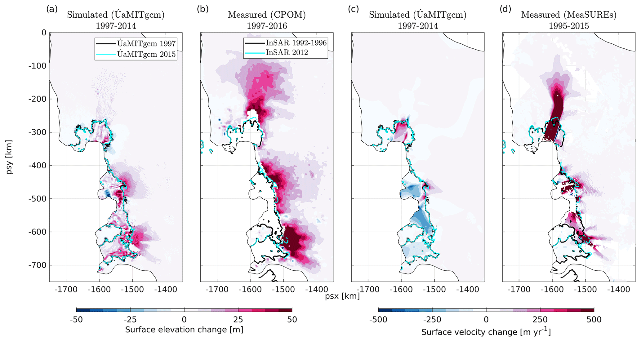
Figure A2A comparison between simulated (a, c) and measured (b, d) changes in surface elevation change and surface velocity changes between 1997 and 2015. Simulated results are from the coupled Úa-MITgcm hindcast experiment var_melt, which starts from an initial ice-sheet geometry representative of the late 1990s–early 2000s and is forced by ocean restoring conditions between 1997 and 2015 (Kimura et al., 2017). Observed changes in surface elevation of the grounded ice between 1997 and 2016 (b) were obtained from CPOM (IMBIE Team, 2018); changes in surface velocity (d) were provided by the MeaSUREs project (Rignot et al., 2017). Grounding line locations in 1997 and 2015 from Úa-MITgcm are shown in panels (a) and (c) in black and cyan, respectively. Corresponding estimates from InSAR data (b, d) were taken from Rignot et al. (2016).
The ice-sheet geometry at the end of the Úa spin-up was transferred to MITgcm and used in a 5-year, ocean-only spin-up with static ice-shelf cavities. This allowed the ocean state to adjust from its uniformly stratified initial conditions to a dynamic state in equilibrium with the varying boundary conditions. The latter conditions correspond to 1992–1996 monthly mean values of temperature, salinity, and velocity from Kimura et al. (2017), linearly interpolated onto the open-ocean boundaries of the regional MITgcm configuration (Fig. 1). Given typical flow speeds of 0.01 m s−1, a 5-year spin-up period was considered to be adequate for the 450 km × 250 km ocean domain with relatively small ice-shelf cavities. At the end of the ocean spin-up (31 December 1996), the coupling between Úa and MITgcm was switched on (Fig. A1), and the coupled configuration was stepped forward with monthly mean ocean restoring conditions between 1 January 1997 and 31 December 2014 based on Kimura et al. (2017). Results from this hindcast experiment, referred to as var_melt, are presented in the next section.
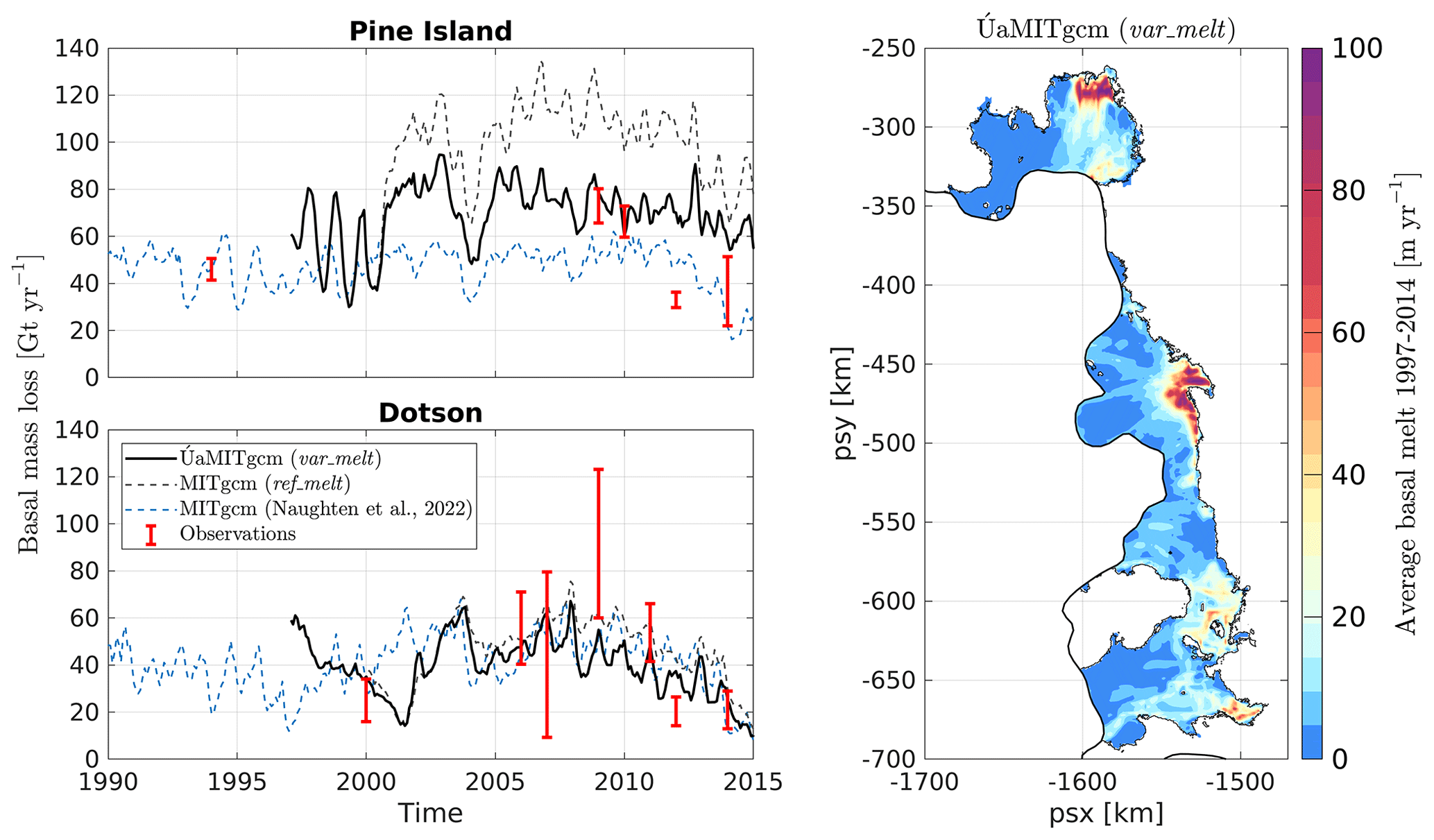
Figure A3A comparison between simulated and measured net basal mass loss for the Pine Island and Dotson ice shelves. Results from the coupled Úa-MITgcm hindcast simulation (var_melt) and two stand-alone MITgcm simulations with fixed cavities (ref_melt and results from Naughten et al. (2022)) are compared to observations for the Pine Island Ice Shelf (years 1994, 2009, 2010, and 2012 from Dutrieux et al. (2014) and 2014 from Heywood et al. (2016)) and the Dotson Ice Shelf (Jenkins et al., 2018). The right panel shows average melt rates between 1997 and 2014 from the var_melt simulation.
A2 Model validation
The performance of Úa-MITgcm in its configuration specific to this study is assessed by comparing model output to available Earth observation and in situ ocean data between January 1997 and December 2014. Whilst model validation is a crucial step towards certifying the model's ability to accurately predict future changes in Antarctic ice volume, a comprehensive validation exercise is not attempted here. It is recognized that further optimization of the current configuration is required in order to eliminate some of the biases that could play a distinctive role in future ice loss projections.
A comparison between modelled and observed changes in ice-sheet surface elevation and surface velocities between 1997 and 2015 is presented in Fig. A2. Whilst Úa-MITgcm simulates widespread negative changes in ice thickness with a spatial pattern that matches the observations, its magnitude and accompanying upstream migration of the grounding line between 1997 and 2015 are significantly underestimated. In agreement with the slower-than-observed changes in ice thickness, changes in surface velocity are smaller than observed. For all ice shelves except the Pine Island Ice Shelf, the simulated change in surface speed has the opposite sign compared to observations. Whilst the sign and magnitude of the observed changes are ultimately simulated at later times in the different Úa-MITgcm perturbation experiments (hi_melt, av_melt, and var_melt in Sect. 2.2), the ice-sheet response is delayed and depends strongly on the ocean forcing. The slower-than-observed response can be caused by a variety of poorly constrained or missing processes, including but not limited to the form of the basal-sliding law, the lack of ice-shelf damage evolution and calving-front migration, and a potential misrepresentation of ocean-induced basal melting in shallow cavities with unknown bathymetry near the grounding line. A quantification of the uncertainties related to these processes and further optimization of the ice–ocean model will be pursued in future studies. In particular, the construction of an initial state that minimizes the misfit between simulated and observed trends in ice thickness and speed over the observational period is an essential requirement for the correct timing of any future mass loss from the West Antarctic Ice Sheet (Goldberg and Holland, 2022).
A comparison between simulated and observed ice-shelf melt rates is provided in Fig. A3. Overall, integrated meltwater fluxes from the coupled hindcast experiment (var_melt) agree well with observations, except for the Pine Island Ice Shelf in 2012 and 2014, when the model overestimates basal mass loss by about 50 %. The temporal variability of var_melt compares favourably to results from Naughten et al. (2022) (dashed blue line in Fig. A3), which include a more complete treatment of ocean–atmosphere interactions. The agreement is not surprising given the fact that the current set-up uses restoring conditions at the ocean boundaries that were obtained from a regional ocean simulation by Kimura et al. (2017), which has a similar model architecture as that of Naughten et al. (2022), and was forced by ERA-Interim atmospheric conditions that are similar to the improved ERA5 atmospheric conditions used in Naughten et al. (2022). The good agreement also holds true despite the absence of ocean surface fluxes in this study, which is an indication that the latter fluxes do not strongly affect the basal-melt variability. Any remaining discrepancies between the current Úa-MITgcm configuration and Naughten et al. (2022), in particular for the Pine Island Glacier, can be caused by a number of differences in ocean parameter choices, cavity geometry, boundary forcing, model resolution, etc., and a detailed comparison will not be pursued here. Results from a stand-alone MITgcm simulation with the same 1997–2014 ocean boundary restoring conditions but with fixed ice-shelf cavities (ref_melt experiment, dashed black line in Fig. A3) produced melt rates for the Pine Island Ice Shelf that were about 50 % higher than results from the corresponding var_melt experiment with evolving cavities. This highlights the important impact of changes in cavity geometry on basal-melt rates and the realization that the calibration of model parameters against observations can lead to distinctly different parameter choices for stand-alone and coupled set-ups.
The spatial distribution of basal melt in the var_melt experiment, averaged between 1997 and 2014, is shown in Fig. A3. Average melt rates in excess of 100 m yr−1 are found near the grounding lines of the Pine Island and Thwaites glaciers, while basal ablation of the Crosson and Dotson ice shelves is generally lower due to lower thermal driving of the far-field ocean (Sect. 4.2). While satellite observation-based estimates of basal-melt rates are available for comparison (Gourmelen et al., 2017; Adusumilli et al., 2018), results are not reproduced here. Significant data gaps remain in regions with the highest melt rates near the grounding lines of the Pine Island and Western Thwaites ice shelves, making it difficult to validate the simulated melt patterns in those regions.
The coupled ice–ocean model Úa-MITgcm is publicly available on GitHub (https://github.com/knaughten/UaMITgcm/, last access: 9 April 2024) and Zenodo (https://doi.org/10.5281/zenodo.7989869, Naughten and De Rydt, 2023), as are the stand-alone components of the ocean circulation model MITgcm (https://github.com/MITgcm/MITgcm/, last access: 9 April 2024) and the ice dynamics model Úa (https://doi.org/10.5281/zenodo.3706623, Gudmundsson, 2020). The configuration files specific to the set-up in this paper are available via https://doi.org/10.5281/zenodo.10778033 (De Rydt, 2024). The scripts that were used to process the Úa and MITgcm output and to produce the figures, as well as original model outputs at the start, middle, and end of all the experiments can be accessed via the same repository (https://doi.org/10.5281/zenodo.10778033, De Rydt, 2024). Data at intermediate times are available upon request from the authors.
The supplement related to this article is available online at: https://doi.org/10.5194/tc-18-1863-2024-supplement.
JDR designed and initiated the project, performed the model simulations, carried out the analysis, and produced the figures and paper. KN coded the latest version of Úa-MITgcm and reviewed and edited the paper.
At least one of the (co-)authors is a member of the editorial board of The Cryosphere. The peer-review process was guided by an independent editor, and the authors also have no other competing interests to declare.
Publisher's note: Copernicus Publications remains neutral with regard to jurisdictional claims made in the text, published maps, institutional affiliations, or any other geographical representation in this paper. While Copernicus Publications makes every effort to include appropriate place names, the final responsibility lies with the authors.
Jan De Rydt is supported by a UKRI Future Leaders Fellowship (grant no. MR/W011816/1) and by the TiPACCs project, which receives funding from the European Union's Horizon 2020 research and innovation programme under grant agreement no. 820575. Kaitlin Naughten is supported by the NERC LTSM project TerraFIRMA. We would like to thank both anonymous reviewers for their support and insightful comments.
This research has been supported by the HORIZON EUROPE European Research Council (grant no. 820575), the UK Research and Innovation (grant no. MR/W011816/1), and NERC (grant no. NE/W004895/1).
This paper was edited by Ginny Catania and reviewed by two anonymous referees.
Adusumilli, S., Fricker, H. A., Medley, B., Padman, L., and Siegfried, M. R.: Interannual variations in meltwater input to the Southern Ocean from Antarctic ice shelves, Nat. Geosci., 13, 616–620, https://doi.org/10.1038/s41561-020-0616-z, 2018. a, b, c, d
Arthern, R. J. and Williams, C. R.: The sensitivity of West Antarctica to the submarine melting feedback, Geophys. Res. Lett., 44, 2352–2359, https://doi.org/10.1002/2017GL072514, 2017. a, b
Bamber, J. L., Gomez-Dans, J. L., and Griggs, J. A.: A new 1 km digital elevation model of the Antarctic derived from combined satellite radar and laser data – Part 1: Data and methods, The Cryosphere, 3, 101–111, https://doi.org/10.5194/tc-3-101-2009, 2009. a
Barnes, J. M., Dias dos Santos, T., Goldberg, D., Gudmundsson, G. H., Morlighem, M., and De Rydt, J.: The transferability of adjoint inversion products between different ice flow models, The Cryosphere, 15, 1975–2000, https://doi.org/10.5194/tc-15-1975-2021, 2021. a
Bradley, A. T., Bett, D. T., Dutrieux, P., De Rydt, J., and Holland, P. R.: The Influence of Pine Island Ice Shelf Calving on Basal Melting, J. Geophys. Res.-Oceans, 127, e2022JC018621, https://doi.org/10.1029/2022JC018621, 2022. a, b, c, d
Cornford, S. L., Martin, D. F., Lee, V., Payne, A. J., and Ng, E. G.: Adaptive mesh refinement versus subgrid friction interpolation in simulations of Antarctic ice dynamics, Ann. Glaciol., 57, 1–9, https://doi.org/10.1017/aog.2016.13, 2016. a
Davison, B. J., Hogg, A. E., Rigby, R., Veldhuijsen, S., van Wessem, J. M., van den Broeke, M. R., Holland, P. R., Selley, H. L., and Dutrieux, P.: Sea level rise from West Antarctic mass loss significantly modified by large snowfall anomalies, Nat. Commun., 14, 1479, https://doi.org/10.1038/s41467-023-36990-3, 2023. a
Depoorter, M. A., Bamber, J. L., Griggs, J. A., Lenaerts, J. T., Ligtenberg, S. R., Van Den Broeke, M. R., and Moholdt, G.: Calving fluxes and basal melt rates of Antarctic ice shelves, Nature, 502, 89–92, https://doi.org/10.1038/nature12567, 2013. a
De Rydt, J.: Model output for “Geometric amplification and suppression of ice-shelf basal melt in West Antarctica” (Version v1), Zenodo [data set], https://doi.org/10.5281/zenodo.10778033, 2024. a, b
De Rydt, J. and Gudmundsson, G. H.: Coupled ice shelf-ocean modeling and complex grounding line retreat from a seabed ridge, J. Geophys. Res. Res.-Earth Surf., 121, 865–880, https://doi.org/10.1002/2015JF003791, 2016. a, b, c
De Rydt, J., Holland, P. R., Dutrieux, P., and Jenkins, A.: Geometric and oceanographic controls on melting beneath Pine Island Glacier, J. Geophys. Res.-Oceans, 119, 2420–2438, https://doi.org/10.1002/2013JC009513, 2014. a
De Rydt, J., Reese, R., Paolo, F. S., and Gudmundsson, G. H.: Drivers of Pine Island Glacier speed-up between 1996 and 2016, The Cryosphere, 15, 113–132, https://doi.org/10.5194/tc-15-113-2021, 2021. a, b, c, d
Dutrieux, P., De Rydt, J., Jenkins, A., Holland, P. R., Ha, H. K., Lee, S. H., Steig, E. J., Ding, Q., Abrahamsen, E. P., and Schröder, M.: Strong sensitivity of pine Island ice-shelf melting to climatic variability, Science, 343, 174–178, https://doi.org/10.1126/science.1244341, 2014. a, b, c, d
Edwards, T. L., Nowicki, S., Marzeion, B., Hock, R., Goelzer, H., Seroussi, H., Jourdain, N. C., Slater, D. A., Turner, F. E., Smith, C. J., McKenna, C. M., Simon, E., Abe-Ouchi, A., Gregory, J. M., Larour, E., Lipscomb, W. H., Payne, A. J., Shepherd, A., Agosta, C., Alexander, P., Albrecht, T., Anderson, B., Asay-Davis, X., Aschwanden, A., Barthel, A., Bliss, A., Calov, R., Chambers, C., Champollion, N., Choi, Y., Cullather, R., Cuzzone, J., Dumas, C., Felikson, D., Fettweis, X., Fujita, K., Galton-Fenzi, B. K., Gladstone, R., Golledge, N. R., Greve, R., Hattermann, T., Hoffman, M. J., Humbert, A., Huss, M., Huybrechts, P., Immerzeel, W., Kleiner, T., Kraaijenbrink, P., Le clec’h, S., Lee, V., Leguy, G. R., Little, C. M., Lowry, D. P., Malles, J. H., Martin, D. F., Maussion, F., Morlighem, M., O’Neill, J. F., Nias, I., Pattyn, F., Pelle, T., Price, S. F., Quiquet, A., Radić, V., Reese, R., Rounce, D. R., Rückamp, M., Sakai, A., Shafer, C., Schlegel, N. J., Shannon, S., Smith, R. S., Straneo, F., Sun, S., Tarasov, L., Trusel, L. D., Van Breedam, J., van de Wal, R., van den Broeke, M., Winkelmann, R., Zekollari, H., Zhao, C., Zhang, T., and Zwinger, T.: Projected land ice contributions to twenty-first-century sea level rise, Nature, 593, 74–82, https://doi.org/10.1038/s41586-021-03302-y, 2021. a, b
Goldberg, D. N. and Holland, P. R.: The Relative Impacts of Initialization and Climate Forcing in Coupled Ice Sheet-Ocean Modeling: Application to Pope, Smith, and Kohler Glaciers, J. Geophys. Res.-Earth Surf., 127, e2021JF006570, https://doi.org/10.1029/2021JF006570, 2022. a, b
Goldberg, D. N., Gourmelen, N., Kimura, S., Millan, R., and Snow, K.: How Accurately Should We Model Ice Shelf Melt Rates?, Geophys. Res. Lett., 46, 189–199, https://doi.org/10.1029/2018GL080383, 2019. a
Gourmelen, N., Goldberg, D. N., Snow, K., Henley, S. F., Bingham, R. G., Kimura, S., Hogg, A. E., Shepherd, A., Mouginot, J., Lenaerts, J. T., Ligtenberg, S. R., and van de Berg, W. J.: Channelized Melting Drives Thinning Under a Rapidly Melting Antarctic Ice Shelf, Geophys. Res. Lett., 44, 9796–9804, https://doi.org/10.1002/2017GL074929, 2017. a
Gudmundsson, G. H.: GHilmarG/UaSource: Ua2019b, Zenodo [code], https://doi.org/10.5281/zenodo.3706623, 2020. a, b
Gudmundsson, G. H., Krug, J., Durand, G., Favier, L., and Gagliardini, O.: The stability of grounding lines on retrograde slopes, The Cryosphere, 6, 1497–1505, https://doi.org/10.5194/tc-6-1497-2012, 2012. a
Gudmundsson, G. H., Paolo, F. S., Adusumilli, S., and Fricker, H. A.: Instantaneous Antarctic ice sheet mass loss driven by thinning ice shelves, Geophys. Res. Lett., 46, 13903–13909, https://doi.org/10.1029/2019GL085027, 2019. a, b
Haseloff, M. and Sergienko, O. V.: The effect of buttressing on grounding line dynamics, J. Glaciol., 64, 417–431, https://doi.org/10.1017/jog.2018.30, 2018. a
Heywood, K. J., Biddle, L. C., Boehme, L., Fedak, M., Dutrieux, P., Jenkins, A., Kaiser, J., Mallett, H., Jones, R. W., Naveira Garabato, A. C., Renfrew, I. A., Stevens, D. P., and Webber, B. G.: Between the devil and the deep blue sea: The role of the Amundsen Sea continental shelf in exchanges between ocean and ice shelves, Oceanography, 29, 118–129, https://doi.org/10.5670/oceanog.2016.104, 2016. a
Holland, D. M. and Jenkins, A.: Modeling thermodynamic ice-ocean interactions at the base of an ice shelf, J. Phys. Oceanogr., 29, 1787–1800, https://doi.org/10.1175/1520-0485(1999)029<1787:mtioia>2.0.co;2, 1999. a
Holland, P. R., Jenkins, A., and Holland, D. M.: The response of Ice shelf basal melting to variations in ocean temperature, J. Climate, 21, 2558–2572, https://doi.org/10.1175/2007JCLI1909.1, 2008. a, b, c
Holland, P. R., O'Connor, G. K., Bracegirdle, T. J., Dutrieux, P., Naughten, K. A., Steig, E. J., Schneider, D. P., Jenkins, A., and Smith, J. A.: Anthropogenic and internal drivers of wind changes over the Amundsen Sea, West Antarctica, during the 20th and 21st centuries, The Cryosphere, 16, 5085–5105, https://doi.org/10.5194/tc-16-5085-2022, 2022. a
Holland, P. R., Bevan, S. L., and Luckman, A. J.: Strong Ocean Melting Feedback During the Recent Retreat of Thwaites Glacier, Geophys. Res. Lett., 50, e2023GL103088, https://doi.org/10.1029/2023GL103088, 2023. a, b, c
IMBIE Team: Mass balance of the Antarctic Ice Sheet from 1992 to 2017, Nature, 558, 219–222, https://doi.org/10.1038/s41586-018-0179-y, 2018. a, b
Jacobs, S. S. and Hellmer, H. H.: Freshening Could Come From Other Melting Ice in the, Observatory, 23, 957–960, 1996. a
Jenkins, A.: A one-dimensional model of ice shelf-ocean interaction, J. Geophys. Res., 96, 20671, https://doi.org/10.1029/91jc01842, 1991. a
Jenkins, A. and Bombosch, A.: Modeling the effects of frazil ice crystals on the dynamics and thermodynamics of Ice Shelf Water plumes, J. Geophys. Res., 100, 6967, https://doi.org/10.1029/94JC03227, 1995. a
Jenkins, A., Nicholls, K. W., and Corr, H. F.: Observation and parameterization of ablation at the base of Ronne Ice Ahelf, Antarctica, J. Phys. Oceanogr., 40, 2298–2312, https://doi.org/10.1175/2010JPO4317.1, 2010. a
Jenkins, A., Dutrieux, P., Jacobs, S., Steig, E. J., Gudmundsson, G. H., Smith, J., and Heywood, K. J.: Decadal ocean forcing and Antarctic ice sheet response: Lessons from the Amundsen Sea, Oceanography, 29, 106–117, https://doi.org/10.5670/oceanog.2016.103, 2016. a
Jenkins, A., Shoosmith, D., Dutrieux, P., Jacobs, S., Kim, T. W., Lee, S. H., Ha, H. K., and Stammerjohn, S.: West Antarctic Ice Sheet retreat in the Amundsen Sea driven by decadal oceanic variability, Nat. Geosci., 11, 733–738, https://doi.org/10.1038/s41561-018-0207-4, 2018. a, b, c
Joughin, I., Smith, B. E., and Schoof, C. G.: Regularized Coulomb Friction Laws for Ice Sheet Sliding: Application to Pine Island Glacier, Antarctica, Geophys. Res. Lett., 46, 4764–4771, https://doi.org/10.1029/2019GL082526, 2019. a
Joughin, I., Shapero, D., Smith, B., Dutrieux, P., and Barham, M.: Ice-shelf retreat drives recent Pine Island Glacier speedup, Sci. Adv., 7, 3080–3091, https://doi.org/10.1126/sciadv.abg3080, 2021. a, b
Jourdain, N. C., Mathiot, P., Merino, N., Durand, G. G., Le Sommer, J., Spence, P., Dutrieux, P., Madec, G., Sommer, J. L., Spence, P., Dutrieux, P., and Madec, G.: Ocean circulation and sea-ice thinning induced by melting ice shelves in the Amundsen Sea, J. Geophys. Res.-Oceans, 122, 2550–2573, https://doi.org/10.1002/2016JC012509, 2017. a
Jourdain, N. C., Mathiot, P., Burgard, C., Caillet, J., and Kittel, C.: Ice Shelf Basal Melt Rates in the Amundsen Sea at the End of the 21st Century, Geophys. Res. Lett., 49, e2022GL100629, https://doi.org/10.1029/2022GL100629, 2022. a, b, c
Kimura, S., Jenkins, A., Regan, H., Holland, P. R., Assmann, K. M., Whitt, D. B., Van Wessem, M., van de Berg, W. J., Reijmer, C. H., and Dutrieux, P.: Oceanographic Controls on the Variability of Ice-Shelf Basal Melting and Circulation of Glacial Meltwater in the Amundsen Sea Embayment, Antarctica, J. Geophys. Res.-Oceans, 122, 10131–10155, https://doi.org/10.1002/2017JC012926, 2017. a, b, c, d, e, f, g
Lazeroms, W. M., Jenkins, A., Rienstra, S. W., and Van De Wal, R. S.: An analytical derivation of ice-shelf basal melt based on the dynamics of meltwater plumes, J. Phys. Oceanogr., 49, 917–939, https://doi.org/10.1175/JPO-D-18-0131.1, 2019. a
Lhermitte, S., Sun, S., Shuman, C., Wouters, B., Pattyn, F., Wuite, J., Berthier, E., and Nagler, T.: Damage accelerates ice shelf instability and mass loss in Amundsen Sea Embayment, P. Natl. Acad. Sci. USA, 117, 24735–24741, https://doi.org/10.1073/pnas.1912890117, 2020. a
Losch, M.: Modeling ice shelf cavities in a z coordinate ocean general circulation model, J. Geophys. Res.-Oceans, 113, https://doi.org/10.1029/2007JC004368, 2008. a, b
Macayeal, D. R.: The basal stress distribution of ice stream E, Antarctica, inferred by control methods, J. Geophys. Res., 97, 595–603, https://doi.org/10.1029/91JB02454, 1992. a
Marshall, J., Hill, C., Perelman, L., and Adcroft, A.: NON-HYDRQ, 102, 5733–5752, 1997. a
Milillo, P., Rignot, E., Rizzoli, P., Scheuchl, B., Mouginot, J., Bueso-Bello, J., and Prats-Iraola, P.: Heterogeneous retreat and ice melt of thwaites glacier, West Antarctica, Sci. Adv., 5, 1–9, https://doi.org/10.1126/sciadv.aau3433, 2019. a
Milillo, P., Rignot, E., Rizzoli, P., Scheuchl, B., Mouginot, J., Bueso-Bello, J. L., Prats-Iraola, P., and Dini, L.: Rapid glacier retreat rates observed in West Antarctica, Nat. Geosci., 15, 48–53, https://doi.org/10.1038/s41561-021-00877-z, 2022. a
Morlighem, M., Rignot, E., Binder, T., Blankenship, D., Drews, R., Eagles, G., Eisen, O., Ferraccioli, F., Forsberg, R., Fretwell, P., Goel, V., Greenbaum, J. S., Gudmundsson, H., Guo, J., Helm, V., Hofstede, C., Howat, I., Humbert, A., Jokat, W., Karlsson, N. B., Lee, W. S., Matsuoka, K., Millan, R., Mouginot, J., Paden, J., Pattyn, F., Roberts, J., Rosier, S., Ruppel, A., Seroussi, H., Smith, E. C., Steinhage, D., Sun, B., Broeke, M. R. d., Ommen, T. D., Wessem, M. v., and Young, D. A.: Deep glacial troughs and stabilizing ridges unveiled beneath the margins of the Antarctic ice sheet, Nat. Geosci., 13, 132–137, https://doi.org/10.1038/s41561-019-0510-8, 2020. a, b, c
Mouginot, J., Rignot, E., and Scheuchl, B.: Sustained increase in ice discharge from the Amundsen Sea Embayment, West Antarctica, from 1973 to 2013, Geophys. Res. Lett., 41, 1576–1584, https://doi.org/10.1002/2013GL059069, 2014. a
Naughten, K. A. and De Rydt, J.: Ua-MITgcm PTDC configuration (Version 1.2), Zenodo [code], https://doi.org/10.5281/zenodo.7989869, 2023. a, b, c
Naughten, K. A., Meissner, K. J., Galton-Fenzi, B. K., England, M. H., Timmermann, R., and Hellmer, H. H.: Future Projections of Antarctic Ice Shelf Melting Based on CMIP5 Scenarios, J. Climate, 31, 5243–5261, https://doi.org/10.1175/JCLI-D-17-0854.s1, 2018. a
Naughten, K. A., De Rydt, J., Rosier, S. H., Jenkins, A., Holland, P. R., and Ridley, J. K.: Two-timescale response of a large Antarctic ice shelf to climate change, Nat. Commun., 12, 1991, https://doi.org/10.1038/s41467-021-22259-0, 2021. a
Naughten, K. A., Holland, P. R., Dutrieux, P., Kimura, S., Bett, D. T., and Jenkins, A.: Simulated Twentieth-Century Ocean Warming in the Amundsen Sea, West Antarctica, Geophys. Res. Lett., 49, e2021GL094566, https://doi.org/10.1029/2021GL094566, 2022. a, b, c, d, e, f, g, h, i
Naughten, K. A., Holland, P. R., and De Rydt, J.: Unavoidable future increase in West Antarctic ice-shelf melting over the twenty-first century, Nat. Clim. Change, 13, 1222–1228, https://doi.org/10.1038/s41558-023-01818-x, 2023. a
Otosaka, I. N., Shepherd, A., Ivins, E. R., Schlegel, N.-J., Amory, C., van den Broeke, M. R., Horwath, M., Joughin, I., King, M. D., Krinner, G., Nowicki, S., Payne, A. J., Rignot, E., Scambos, T., Simon, K. M., Smith, B. E., Sørensen, L. S., Velicogna, I., Whitehouse, P. L., A, G., Agosta, C., Ahlstrøm, A. P., Blazquez, A., Colgan, W., Engdahl, M. E., Fettweis, X., Forsberg, R., Gallée, H., Gardner, A., Gilbert, L., Gourmelen, N., Groh, A., Gunter, B. C., Harig, C., Helm, V., Khan, S. A., Kittel, C., Konrad, H., Langen, P. L., Lecavalier, B. S., Liang, C.-C., Loomis, B. D., McMillan, M., Melini, D., Mernild, S. H., Mottram, R., Mouginot, J., Nilsson, J., Noël, B., Pattle, M. E., Peltier, W. R., Pie, N., Roca, M., Sasgen, I., Save, H. V., Seo, K.-W., Scheuchl, B., Schrama, E. J. O., Schröder, L., Simonsen, S. B., Slater, T., Spada, G., Sutterley, T. C., Vishwakarma, B. D., van Wessem, J. M., Wiese, D., van der Wal, W., and Wouters, B.: Mass balance of the Greenland and Antarctic ice sheets from 1992 to 2020, Earth Syst. Sci. Data, 15, 1597–1616, https://doi.org/10.5194/essd-15-1597-2023, 2023. a
Paolo, F. S., Fricker, H. A., and Padman, L.: Volume loss from Antarctic ice shelves is accelerating, Science, 348, 327–331, https://doi.org/10.1126/science.aaa0940, 2015. a
Paolo, F. S., Gardner, A. S., Greene, C. A., Nilsson, J., Schodlok, M. P., Schlegel, N.-J., and Fricker, H. A.: Widespread slowdown in thinning rates of West Antarctic ice shelves, The Cryosphere, 17, 3409–3433, https://doi.org/10.5194/tc-17-3409-2023, 2023. a, b
Patmore, R. D., Holland, P. R., Munday, D. R., Naveira Garabato, A. C., Stevens, D. P., Meredith, M. P., Patmore, R. D., Holland, P. R., Munday, D. R., Garabato, A. C. N., Stevens, D. P., and Meredith, M. P.: Topographic Control of Southern Ocean Gyres and the Antarctic Circumpolar Current: A Barotropic Perspective, J. Phys. Oceanogr., 49, 3221–3244, https://doi.org/10.1175/JPO-D-19-0083.1, 2019. a, b
Pattyn, F., Schoof, C., Perichon, L., Hindmarsh, R. C. A., Bueler, E., de Fleurian, B., Durand, G., Gagliardini, O., Gladstone, R., Goldberg, D., Gudmundsson, G. H., Huybrechts, P., Lee, V., Nick, F. M., Payne, A. J., Pollard, D., Rybak, O., Saito, F., and Vieli, A.: Results of the Marine Ice Sheet Model Intercomparison Project, MISMIP, The Cryosphere, 6, 573–588, https://doi.org/10.5194/tc-6-573-2012, 2012. a
Pedersen, F. B.: Dense bottom currents in rotating ocean, J. Hydraul. Div. Am. Soc. Civ. Eng., 106, 1291–1308, 1980. a
Pegler, S. S.: Marine ice sheet dynamics: The impacts of ice-shelf buttressing, J. Fluid Mech., 857, 605–647, https://doi.org/10.1017/jfm.2018.741, 2018. a
Pritchard, H. D., Ligtenberg, S. R., Fricker, H. A., Vaughan, D. G., Van Den Broeke, M. R., and Padman, L.: Antarctic ice-sheet loss driven by basal melting of ice shelves, Nature, 484, 502–505, https://doi.org/10.1038/nature10968, 2012. a
Reese, R., Garbe, J., Hill, E. A., Urruty, B., Naughten, K. A., Gagliardini, O., Durand, G., Gillet-Chaulet, F., Gudmundsson, G. H., Chandler, D., Langebroek, P. M., and Winkelmann, R.: The stability of present-day Antarctic grounding lines – Part 2: Onset of irreversible retreat of Amundsen Sea glaciers under current climate on centennial timescales cannot be excluded, The Cryosphere, 17, 3761–3783, https://doi.org/10.5194/tc-17-3761-2023, 2023. a
Rignot, E., Thomas, R. H., Kanagaratnam, P., Casassa, G., Frederick, E., Gogineni, S., Krabill, W., Rivera, A., Russell, R., Sonntag, J., Swift, R., and Yungel, J.: Improved estimation of the mass balance of glaciers draining into the Amundsen Sea sector of West Antarctica from the CECS/NASA 2002 campaign, Ann. Glaciol., 39, 231–237, https://doi.org/10.3189/172756404781813916, 2004. a
Rignot, E., Mouginot, J., and Scheuchl, B.: MEaSUREs Antarctic Grounding Line from Differential Satellite Radar Interferometry, Version 2, Bouler, Colorado USA, NASA National Snow and Ice Data Center Distributed Active Archive Center [data set], https://doi.org/10.5067/D7GK8F5J8M8R, 2016. a, b
Rignot, E., Mouginot, J., and Scheuchl, B.: MEaSUREs InSAR-Based Antarctica Ice Velocity Map, Version 2, Boulder, Colorado USA, NASA National Snow and Ice Data Center Distributed Active Archive Center [data set], https://doi.org/10.5067/IKBWW4RYHF1Q, 2017. a
Rignot, E., Mouginot, J., Scheuchl, B., Van Den Broeke, M., Van Wessem, M. J., and Morlighem, M.: Four decades of Antarctic ice sheet mass balance from 1979–2017, P. Natl. Acad. Sci. USA, 116, 1095–1103, https://doi.org/10.1073/pnas.1812883116, 2019. a, b, c
Seroussi, H. and Morlighem, M.: Representation of basal melting at the grounding line in ice flow models, The Cryosphere, 12, 3085–3096, https://doi.org/10.5194/tc-12-3085-2018, 2018. a
Seroussi, H., Nowicki, S., Simon, E., Abe-Ouchi, A., Albrecht, T., Brondex, J., Cornford, S., Dumas, C., Gillet-Chaulet, F., Goelzer, H., Golledge, N. R., Gregory, J. M., Greve, R., Hoffman, M. J., Humbert, A., Huybrechts, P., Kleiner, T., Larour, E., Leguy, G., Lipscomb, W. H., Lowry, D., Mengel, M., Morlighem, M., Pattyn, F., Payne, A. J., Pollard, D., Price, S. F., Quiquet, A., Reerink, T. J., Reese, R., Rodehacke, C. B., Schlegel, N.-J., Shepherd, A., Sun, S., Sutter, J., Van Breedam, J., van de Wal, R. S. W., Winkelmann, R., and Zhang, T.: initMIP-Antarctica: an ice sheet model initialization experiment of ISMIP6, The Cryosphere, 13, 1441–1471, https://doi.org/10.5194/tc-13-1441-2019, 2019. a
Seroussi, H., Nowicki, S., Payne, A. J., Goelzer, H., Lipscomb, W. H., Abe-Ouchi, A., Agosta, C., Albrecht, T., Asay-Davis, X., Barthel, A., Calov, R., Cullather, R., Dumas, C., Galton-Fenzi, B. K., Gladstone, R., Golledge, N. R., Gregory, J. M., Greve, R., Hattermann, T., Hoffman, M. J., Humbert, A., Huybrechts, P., Jourdain, N. C., Kleiner, T., Larour, E., Leguy, G. R., Lowry, D. P., Little, C. M., Morlighem, M., Pattyn, F., Pelle, T., Price, S. F., Quiquet, A., Reese, R., Schlegel, N.-J., Shepherd, A., Simon, E., Smith, R. S., Straneo, F., Sun, S., Trusel, L. D., Van Breedam, J., van de Wal, R. S. W., Winkelmann, R., Zhao, C., Zhang, T., and Zwinger, T.: ISMIP6 Antarctica: a multi-model ensemble of the Antarctic ice sheet evolution over the 21st century, The Cryosphere, 14, 3033–3070, https://doi.org/10.5194/tc-14-3033-2020, 2020. a
Shepherd, A., Gilbert, L., Muir, A. S., Konrad, H., McMillan, M., Slater, T., Briggs, K. H., Sundal, A. V., Hogg, A. E., and Engdahl, M. E.: Trends in Antarctic Ice Sheet Elevation and Mass, Geophys. Res. Lett., 46, 8174–8183, https://doi.org/10.1029/2019GL082182, 2019. a
Siahaan, A., Smith, R. S., Holland, P. R., Jenkins, A., Gregory, J. M., Lee, V., Mathiot, P., Payne, A. J. ., Ridley, J. K. ., and Jones, C. G.: The Antarctic contribution to 21st-century sea-level rise predicted by the UK Earth System Model with an interactive ice sheet, The Cryosphere, 16, 4053–4086, https://doi.org/10.5194/tc-16-4053-2022, 2022. a, b
Silvano, A., Holland, P. R., Naughten, K. A., Dragomir, O., Dutrieux, P., Jenkins, A., Si, Y., Stewart, A. L., Peña Molino, B., Janzing, G. W., Dotto, T. S., and Naveira Garabato, A. C.: Baroclinic Ocean Response to Climate Forcing Regulates Decadal Variability of Ice-Shelf Melting in the Amundsen Sea, Geophys. Res. Lett., 49, e2022GL100646, https://doi.org/10.1029/2022GL100646, 2022. a
Smith, B., Fricker, H. A., Gardner, A. S., Medley, B., Nilsson, J., Paolo, F. S., Holschuh, N., Adusumilli, S., Brunt, K., Csatho, B., Harbeck, K., Markus, T., Neumann, T., Siegfried, M. R., and Zwally, H. J.: Pervasive ice sheet mass loss reflects competing ocean and atmosphere processes, Science, 368, 1239–1242, https://doi.org/10.1126/science.aaz5845, 2020. a
Smith, J. A., Andersen, T. J., Shortt, M., Gaffney, A. M., Truffer, M., Stanton, T. P., Bindschadler, R., Dutrieux, P., Jenkins, A., Hillenbrand, C. D., Ehrmann, W., Corr, H. F., Farley, N., Crowhurst, S., and Vaughan, D. G.: Sub-ice-shelf sediments record history of twentieth-century retreat of Pine Island Glacier, Nature, 541, 77–80, https://doi.org/10.1038/nature20136, 2017. a
Surawy-Stepney, T., Hogg, A. E., Cornford, S. L., and Davison, B. J.: Episodic dynamic change linked to damage on the thwaites glacier ice tongue, Nat. Geosci., 16, 37–43, https://doi.org/10.1038/s41561-022-01097-9, 2023. a
Timmermann, R. and Hellmer, H. H.: Southern Ocean warming and increased ice shelf basal melting in the twenty-first and twenty-second centuries based on coupled ice-ocean finite-element modelling, Ocean Dynam., 63, 1011–1026, https://doi.org/10.1007/s10236-013-0642-0, 2013. a
van Wessem, J. M., van de Berg, W. J., Noël, B. P. Y., van Meijgaard, E., Amory, C., Birnbaum, G., Jakobs, C. L., Krüger, K., Lenaerts, J. T. M., Lhermitte, S., Ligtenberg, S. R. M., Medley, B., Reijmer, C. H., van Tricht, K., Trusel, L. D., van Ulft, L. H., Wouters, B., Wuite, J., and van den Broeke, M. R.: Modelling the climate and surface mass balance of polar ice sheets using RACMO2 – Part 2: Antarctica (1979–2016), The Cryosphere, 12, 1479–1498, https://doi.org/10.5194/tc-12-1479-2018, 2018. a, b
Weertman, J.: Stability of the Junction of an Ice Sheet and an Ice Shelf, J. Glaciol., 13, 3–11, https://doi.org/10.3189/s0022143000023327, 1974. a
Zhao, K. X., Stewart, A. L., and McWilliams, J. C.: Sill-Influenced Exchange Flows in Ice Shelf Cavities, J. Phys. Oceanogr., 49, 163–191, https://doi.org/10.1175/JPO-D-18-0076.1, 2019. a
- Abstract
- Introduction
- Numerical set-up and experiments
- Cavity transfer coefficients
- Ice–ocean feedbacks in the absence of far-field ocean variability
- The importance of far-field ocean variability
- Glaciological implications
- Summary and conclusions
- Appendix A: Model initialization and validation
- Code and data availability
- Author contributions
- Competing interests
- Disclaimer
- Acknowledgements
- Financial support
- Review statement
- References
- Supplement