the Creative Commons Attribution 4.0 License.
the Creative Commons Attribution 4.0 License.
 | 09 Apr 2024
A rigorous approach to the specific surface area evolution in snow during temperature gradient metamorphism
Anna Braun
Kévin Fourteau
Despite being one of the most fundamental microstructural parameters of snow, the specific surface area (SSA) dynamics during temperature gradient metamorphism (TGM) have so far been addressed only within empirical modeling. To surpass this limitation, we propose a rigorous modeling of SSA dynamics using an exact equation for the temporal evolution of the surface area, fed by pore-scale finite-element simulations of the water vapor field coupled with the temperature field on X-ray computed tomography images. The proposed methodology is derived from the first principles of physics and thus does not rely on any empirical parameter. Since the calculated evolution of the SSA is highly sensitive to fluctuations in the experimental data, we quantify the impact of these fluctuations within a stochastic error model. In our simulations, the only poorly constrained physical parameter is the condensation coefficient α. We address this problem by simulating the SSA evolution for a wide range of α values and estimate optimal values by minimizing the differences between simulations and experiments. This methodology suggests that α lies in the intermediate range and slightly varies between experiments. Also, our results suggest a transition of the value of α in one TGM experiment, which can be explained by a transition in the underlying surface morphology. Overall, we are able to reproduce very subtle variations in the SSA evolution with correlations of R2=0.95 and 0.99, respectively, for the two TGM time series considered. Finally, our work highlights the necessity of including kinetic effects and of using realistic microstructures to comprehend the evolution of SSA during TGM.
- Article
(5157 KB) - Full-text XML
- BibTeX
- EndNote


The specific surface area (SSA) of snow is the interface area between ice and air in the microstructure of porous snow, normalized per volume. The SSA is a crucial parameter for the optical albedo of snow (Dumont et al., 2014), fluid permeability (Zermatten et al., 2014), avalanche prediction (Schweizer et al., 2003), microwave remote sensing (Picard et al., 2022), or chemical exchange with the atmosphere (Hanot and Dominé, 1999). The SSA evolution in time is one key to quantifying metamorphism (Legagneux et al., 2004; Domine et al., 2007; Pinzer et al., 2012; Wang and Baker, 2014; Harris Stuart et al., 2023) and needs to be faithfully parameterized in snow cover models to capture the evolution of physical properties. Temperature gradient metamorphism (TGM) is by far the most important type of metamorphism in dry, natural snow covers (Schneebeli and Sokratov, 2004; Legagneux et al., 2004) since gradient-free (i.e., isothermal) conditions exist at most in deep polar firn. However, a detailed physical understanding of the SSA evolution under TGM is still lacking.
Detailed experimental data on TGM can be conveniently acquired nowadays through X-ray micro-computed tomography (μCT). Imaging of snow samples with μCT has been developed over the last 2 decades (Coleou et al., 2001; Flin et al., 2004; Schneebeli and Sokratov, 2004; Schleef and Loewe, 2013) and provides a 3D insight into the microstructure that is otherwise invisible to the naked eye. In contrast to many destructive snow measurement methods, μCT preserves the structure of the snow. Since the entire snow microstructure is available, any parameter of interest, especially SSA, can be computed within well-characterized uncertainties due to reconstruction and image analysis (Hagenmuller et al., 2016). Using instrumented sample holders to constrain temperatures and temperature gradients, in situ time-lapse observations of the microstructure during TGM are obtained (Kaempfer et al., 2005; Pinzer et al., 2012; Calonne et al., 2014a; Hammonds et al., 2015; Wiese and Schneebeli, 2017; Li and Baker, 2022). While many SSA evolution curves originated from these studies, none of them have been convincingly reproduced from a physical model.
Physical models of snow metamorphism must comply with the ice crystal growth dynamics at the pore scale (Krol and Löwe, 2016), which include heat and mass diffusion, accommodated by attachment kinetics controlling the deposition and sublimation of water molecules onto the ice lattice (Colbeck, 1983; Libbrecht, 2005). Secondary effects on the temporal SSA evolution might be expected from other processes like mechanical deformation (Wang and Baker, 2013; Schleef et al., 2014) and advection of air in terms of porosity (Ebner et al., 2016; Jafari et al., 2022). In this picture, one key parameter driving snow metamorphism is the condensation coefficient α, also called the attachment, kinetic, or sticking coefficient (Libbrecht, 2005; Kaempfer and Plapp, 2009; Krol and Löwe, 2016; Demange et al., 2017; Fourteau et al., 2021b; Bouvet et al., 2022), that controls the kinetics of vapor deposition and sublimation. The condensation coefficient is applicable at the micrometer scale of ambient diffusion processes and thereby subsumes the underlying nanoscale kinetics resulting from the molecular dynamics on the surface of the ice crystal lattice (Saito, 1996). Many measurement and modeling attempts carefully characterize α for ice crystals (Libbrecht, 2005; Hobbs, 2010; Barrett et al., 2012; Libbrecht and Rickerby, 2013; Pokrifka et al., 2020). Nevertheless, α is experimentally challenging to constrain even for isolated crystal growth. One reason for this is the fundamental experimental difficulty of inverting growth data as soon as diffusion is involved (Libbrecht, 2005). The other reason is that α depends on numerous effects such as temperature, supersaturation, and crystallographic orientation (Saito, 1996; Libbrecht, 2005). The large variations between basal and prismatic surface kinetics are, for example, the key to snow crystal morphology (Barrett et al., 2012). The situation is even more complicated in the snow cover, where many different surface orientations exist simultaneously (Granger et al., 2021). Therefore, the kinetics is more difficult to assess in snow, and only a few studies exist constraining α from the comparison of μCT-based simulations with experiments (Bouvet et al., 2022; Fourteau et al., 2021a). Thus, α constitutes the great unknown in snow metamorphism as is commonly stressed in TGM models (Miller and Adams, 2009; Kaempfer and Plapp, 2009; Calonne et al., 2014b).
Model attempts characterizing TGM can be classified by their treatment of attachment kinetics and whether the microstructure is taken from μCT or geometrically idealized. Using μCT images, Flin and Brzoska (2008) calculated deposition fluxes in the absence of kinetics under the assumption of local equilibrium at the interface (diffusion-limited growth). A similar approximation was used in Krol and Löwe (2016) to relate the temperature-gradient-driven deposition fluxes to measured, local interface velocities. The latter can be considered a generalization of the (diffusion-limited) air bubble migration under a temperature gradient in ice (Shreve, 1967) to complex geometries. However, the assumption of purely diffusion-limited growth has already been questioned (Krol and Löwe, 2018) due to contradictions with the measured SSA evolution. The μCT-based theoretical homogenization (Calonne et al., 2014b), in contrast, applies to the slow kinetic (i.e., kinetics-limited) regime. The intermediate regime between the diffusion-limited to kinetics-limited vapor transport under a temperature gradient was numerically analyzed in Fourteau et al. (2021a), where the latter approach was physically similar to the phase field model (Kaempfer and Plapp, 2009). Since the choice of α has a significant impact on numerical effort, it is not surprising that the majority of modeling attempts exist for simplified geometries (mostly spheres) (Adams and Brown, 1982; Colbeck, 1983; Albert and McGilvary, 1992; Miller and Adams, 2009) at the expense of microstructural realism. The most widely used models for predicting the SSA evolution under TGM are those implemented in snow cover models, e.g., Flanner and Zender (2006). Like other simplified models, Flanner and Zender (2006) neglect kinetics and employ diffusion-limited growth for the distribution of spherical particles. Due to the involved empirical parameters (mean sphere radius and spacing), which prevent an unambiguous mapping onto arbitrary microstructures, validating these models through μCT laboratory experiments would remain inconclusive.
In principle, no empiricism is required, and the SSA evolution for arbitrary 3D microstructure can be computed exactly (Krol and Löwe, 2018), as long as the required parameters are supplied. The surface area equation is rigorously formulated on the basis of a growth rate that can be computed from the interfacial curvature and the interface velocity (vn) after surface averaging. While the interfacial curvature is a purely geometrical quantity that can directly be computed from a μCT image, vn is a physical quantity that further depends on the involved physical processes. In this framework, any model that predicts vn to be the result of 3D heat and mass diffusion with interface kinetics could be employed here – that is, either phase field models (Kaempfer and Plapp, 2009) or diffusion models (Fourteau et al., 2021b). The two are equivalent in view of the involved physics and only differ in their representation of the interface. This route to the SSA evolution in TGM is rigorous (apart from numerical approximations) but has never been pursued before. Advancing on this route is the aim of the present work. To this end, we combine a finite-element (FE) solution of the pore-scale heat and mass diffusion equations following Fourteau et al. (2021b) with the exact surface area equation from Krol and Löwe (2018) in order to reproduce the SSA evolution during TGM from the four-dimensional (4D) μCT image data from Pinzer et al. (2012).
The paper is organized as follows. The theoretical background for pore-scale diffusion and the SSA is presented in Sect. 2. In Sect. 3, we describe the numerical procedures (meshing, FE solution, and image processing), a simple stochastic error analysis, and the validation of our numerical workflow against an analytical solution. The simulations for the TGM time series are shown in Sect. 4 and discussed in Sect. 5.
2.1 Heat and vapor transfer at the pore scale
For an arbitrary snow structure, morphological changes during metamorphism are predominantly driven by the coupled diffusion of heat and mass, together with ice–air interface evolution, due to deposition and sublimation of vapor. In the following, we closely follow the descriptions by Kaempfer and Plapp (2009), Calonne et al. (2014b), Krol and Löwe (2016), and Fourteau et al. (2021a). We consider a representative snow volume at the microscale consisting of ice and air and denote the subdomains occupied by the ice and air phases by Ωi and Ωa, respectively. In the following, subscripts i and a denote quantities which are defined in the respective domains Ωi and Ωa. Due to the separation of timescales between heat and mass diffusion in the pores and the evolution of the interface, we employ the common assumption of a small particle Péclet number (Libbrecht, 2005) and consider stationary heat and mass diffusion equations (i.e., Laplace equations). Furthermore, we neglect the influence of mechanical deformation as is usually done in pore-scale metamorphism models (e.g., Calonne et al., 2014b; Krol and Löwe, 2016). We also neglect the potential presence of convection and air advection in the pore space. These assumptions are consistent with the experimental data used in this article, obtained under controlled laboratory conditions (Pinzer et al., 2012). They are also good candidates in terms of minimum-required complexity to model SSA evolution from pore-scale physics. The partial density of water vapor in air, ρv, and the ice and air temperatures, Ti and Ta, respectively, are governed by
where Dv is the vapor diffusion constant in air, and κi and κa are the thermal diffusivities of ice and air, respectively.
The heat and mass diffusion equations are coupled via boundary conditions on the ice–air interface Γ. The mass conservation at the ice–air interface is linked to the water vapor concentration by a Stefan-type condition:
where ρi denotes the ice density; n is the unit normal vector field on Γ, which is oriented into the pore space Ωa; and vn is the interface velocity on Γ in the direction of n. The velocity vn is therefore positive for deposition and negative for sublimation.
The conservation of energy requires the continuity of temperature and heat flux on the ice–air interface according to
As per Krol and Löwe (2016), the latent heat during the sublimation and deposition is neglected for reduced model complexity. Since mass and energy conservation involves the unknown interface velocity vn, the internal boundary conditions must be completed by a constitutive law that characterizes vn during crystal growth. Here, we employ the Hertz–Knudsen law (Libbrecht, 2005; Kaempfer and Plapp, 2009; Fourteau et al., 2021a), which includes the impact of interfacial curvature on the equilibrium vapor concentration (Gibbs–Thomson effect) according to
The equilibrium (or saturation) vapor concentration on a flat surface at temperature T is denoted by ρv,s(T), the capillary length by d0, the mean curvature by H, the condensation coefficient by α, and the kinetic velocity by vkin. The capillary length is related to , where γ is the interfacial free energy, a is the mean intermolecular spacing of water molecules in ice, and kB is the Boltzmann constant. The kinetic velocity is defined here as , with the mass of water molecule m. This definition follows Fourteau et al. (2021a) and thus differs from the definition in Libbrecht (2005). In the Hertz–Knudsen equation, the condensation coefficient α is defined as the probability of a water molecule sticking to a surface after impinging on it. Therefore, values in the range [0,1] are commonly desired, where α→0 corresponds to slow surface kinetics, and for α≈1 the diffusion-dominated regime is attained (Libbrecht, 2005; Fourteau et al., 2021a). Mathematically the equation remains well defined also for α>1, which may be physically interpreted as a deviation from the local constitutive behavior (Eq. 7) due to non-local surface processes (Libbrecht, 2005). Although α is known to depend on temperature, supersaturation, and crystallographic orientation and to vary on different parts of the ice–air interface (Libbrecht, 2005), we rely on the simplifying assumption of a single and constant α value. It should thus rather be understood as an effective condensation coefficient.
2.2 Evolution of SSA
In this article, we use two SSA definitions: specific surface area per unit volume s and specific surface area per ice volume SSAV. They are closely related through the ice volume fraction ϕi:
We mainly work with the quantity s for the rest of the article. However, we note that the quantity SSAV is more commonly used in the snow community (e.g., Matzl and Schneebeli, 2006) since it directly corresponds to the optical diameter.
The solution of the heat and mass diffusion equations (Eqs. 1–3) with boundary conditions (Eqs. 4–7) yields the spatially varying interface velocity vn at any point on the ice–air interface Γ. As shown by Drew (1990) and Krol and Löwe (2018), this information, together with information about surface curvature, is sufficient to calculate the evolution of the SSA rigorously via surface averaging. As a result, for single grains or statistically homogeneous microstructures, the surface area evolution equation can be expressed as follows:
Here, the term , referred to as the growth rate in this article, is the product of the local interface velocity vn and the local mean curvature H averaged over the ice–air interface area (the surface average being indicated by an overline over the product). Equation (9) is a linear homogeneous first-order ordinary differential equation and can be formally solved in closed form by the separation of variables, yielding
Equation (10) allows us to compute the SSA evolution from the growth rate , which must be computed from the solution of the 3D diffusion problem. This link between the SSA evolution and the heat and mass diffusion equations is rigorous.
The end goal of our numerical modeling is to simulate the SSA decrease in snow samples over time based on the pore-scale physics and to compare this decrease to experimental observations. For that, we rely on time-resolved μCT images that were obtained under TGM conditions (Pinzer et al., 2012). These μCT scans provide (i) experimental data of the evolution of the SSA over time and (ii) snow microstructures that can be used for our physical modeling. The computation of a vapor field using an FE simulation, combined with the local curvature of the snow sample, allows us to estimate over a given snow microstructure. With Eq. (9), this yields the evolution of the SSA during a given time interval.
As we want to reproduce the SSA evolution of entire time series, our general workflow is as follows. For a given experimental time series, we initialize the first term s1 of the simulated SSA values using the SSA deduced from the first μCT image of the experimental time series. Then, the second simulated SSA value s2 is computed by applying the growth rate deduced from an FE simulation performed on the first μCT image. The procedure is then repeated to compute the nth term of the simulated SSA sn using the already known value sn−1 and an FE simulation performed on the (n−1)th μCT image. The workflow and its different steps are detailed in the sections below and illustrated in Fig. 1.
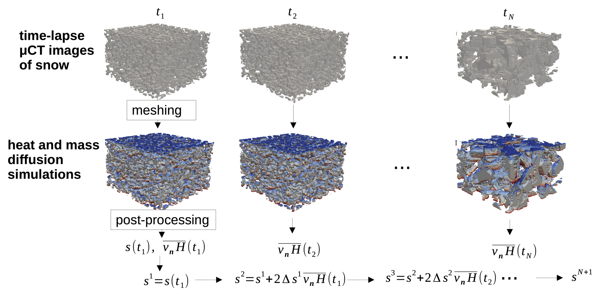
Figure 1Schematic illustration of the workflow used in this study in order to compute the modeled SSA values . For each 3D image of a μCT time-lapse series, a tetrahedral mesh is produced and a heat and mass diffusion simulation is conducted. The simulated interface growth velocity vn is displayed in color in the figure (blue corresponding to a receding interface and red to a growing interface). In the post-processing step, the growth rates are extracted and used to model the SSA evolution according to Eq. (18).
3.1 μCT time-lapse experiments
The numerical simulations were conducted on 4D image data of two TGM experiments (series 1 and 2), which were previously acquired and have already been analyzed in Pinzer et al. (2012) and Krol and Löwe (2016). In the experiments, a constant temperature gradient was applied by adjusting a snow sample's bottom and top temperatures in an instrumented tomography sample holder known as Snowbreeder (Pinzer and Schneebeli, 2009a). Series 1 lasted 384 h, while series 2 lasted 665 h. The mean temperature T of the sample and the temperature gradient ∇T are similar for both series: °C and ∇T=47 K m−1 for series 1 and °C and ∇T=55 K m−1 for series 2. Both time series start from rounded grains with slightly different initial values of SSA and volumetric density, namely SSA mm−1 and for series 1 and SSA mm−1 and for series 2. For further experimental details, we refer to Pinzer et al. (2012).
The μCT image data were taken from the snow sample every 8 h in time-lapse mode and segmented into binary images as described previously (Pinzer et al., 2012). These binary images are denoted by
at different time steps and are voxel images with voxel length of m in series 1 and of m in series 2. This corresponds to samples of mm3 for series 1 and mm3 for series 2. Both series show the commonly observed decay of SSA (Taillandier et al., 2007; Pinzer and Schneebeli, 2009b; Calonne et al., 2014a).
3.2 FE solution of temperature and vapor fields
3.2.1 Meshing
The production of an appropriate mesh that discretizes the air and ice domains, preserves the ice–air interface, and is fine enough to get accurate numerical solution (without overloading computational resources) is a key requirement for our problem. To this end, we employ the open-source Computational Geometry Algorithms Library (CGAL) (The CGAL Project, 2022). Specifically, we use the class Polyhedral_mesh_domain_with_features_3 that implements a tetrahedral meshing of a domain bounded by polyhedral surfaces, which are preserved during the meshing process. The provided surfaces need to be closed and free of self-intersections. To obtain such surfaces, we extract the ice–air interface from the binary μCT data (Eqs. 11, 12) following the procedure from Krol and Löwe (2018), by applying a Gaussian smoothing and the contour filter from the Visualization Toolkit (VTK) (Schroeder et al., 2006). However, by default, this procedure applied to μCT images yields a surface that is open at the boundaries of the domain. In order to obtain closed surfaces, we added a small air padding (3 voxels thick) around the image. This allowed us to properly define a closed outer boundary suitable for meshing. As detailed below, we provided special care to ensure that the introduction of this artificial air padding does not perturb the simulation within the snow microstructure itself. Mesh_Criteria_3 parameters control the meshing algorithm in CGAL; mesh tetrahedra are regulated by the radius–edge ratio upper bound of 1.5 and circumradius upper bound of 3 voxels, and triangles in the boundary surface mesh are regulated by the lower angular bound of 25° and radius upper bound of 0.75 voxels. These mesh parameters were manually fine-tuned through visual inspection. We estimated the sensitivity of our results to the mesh parameters. We found that doubling the number of elements in the mesh impacted the simulated growth rate by about 10 %. This is small in light of the dependence of the SSA values on the condensation coefficient α investigated in this study. Moreover, the very good agreement between an FE simulation and the analytical solution for a spherical problem (see Sect. 3.5) suggests that our meshing criteria yield an appropriate mesh. We save the mesh in four files listing the nodes, bulk elements, boundary elements, and header information, defining a mesh in the format of the FE software Elmer (Malinen and Råback, 2013). In addition, we computed the boundary weight at each mesh node k of the triangulated ice–air interface Γh:
where ψk is the basis function assigned to the node k so that the sum of all boundary weights ωk gives the area of the whole boundary surface. Saving boundary weights is substantial for the computation of the interface velocities as surface integrals over the solution of heat and mass diffusion equations. For consistency and accuracy, employing the same integration scheme that underlies the FE solution is advantageous.
The FE meshes of this article are based on all the available μCT images. We verified that these selected volumes were large enough to yield representative results. By varying the sub-volumes extracted from the center of μCT images at the start and the end of both series (I(t1), I(t49), , and ), we found that the simulated growth rate corresponds to a representative value for the sample sizes used in this study. This is consistent with the results of Calonne et al. (2011) for thermal conductivity, who report representativeness for sample side lengths of between 2.5 and 5 mm.
3.2.2 FE solution
On the tetrahedral FE mesh with a preserved surface, we solve heat and mass diffusion equations (Eqs. 1–3) employing the open-source FE software Elmer (Malinen and Råback, 2013). For the simulation, we need to apply a given temperature gradient across the snow microstructure. However, due to the presence of artificial air padding, directly applying the required temperature gradient across the whole FE mesh (snow plus air padding around the image) would result in a smaller temperature gradient within the snow itself (as the air is less conductive than the snow and thus concentrates the temperature gradient). In order to obtain the proper temperature gradient across the snow microstructure, the simulations are performed in two consecutive steps. First, the heat diffusion equation is solved over the whole FE mesh (snow plus air padding around the image), and its result is used to estimate how a temperature gradient applied over the whole FE mesh translates into a temperature gradient within the snow microstructure itself. This allows us to determine a corrected temperature gradient to be applied over the whole FE mesh in order to obtain the desired temperature gradient in the snow. This corrected temperature gradient is then used to solve the heat and mass diffusion equations with the appropriate temperature gradient across the snow microstructure. For the computation of heat and mass diffusion equations, we use the standard Elmer solvers HeatSolver and AdvectionDiffusionSolver following Fourteau et al. (2021a). The equations are solved with the iterative biconjugate gradient stabilized method (BiCGSTAB; Van der Vorst, 1992) with an incomplete lower–upper (ILU) preconditioner, meant to facilitate the numerical solving by performing an incomplete LU factorization (Saad, 2003). The maximum number of iterations is set to 2000, and the convergence tolerance is set to 10−10 for the heat diffusion equation and to 10−12 for the mass diffusion equation. The correct temperature gradient across the domain is applied by setting top and bottom temperatures to
where T and ∇T are the experimental temperature and temperature gradient, respectively, and h is the total height of the sample.
For the vapor boundary condition, we combine the Stefan condition (Eq. 4) by neglecting the ρvvn term due to ρv≪ρi and the Gibbs–Thomson equation (Eq. 7) to obtain a Robin boundary condition at the ice–air interface:
Here, the equilibrium water vapor concentration is given by the Clausius–Clapeyron relation, corrected for the Gibbs–Thomson effect (Fourteau et al., 2021a):
where M is the molar mass of water, R is the ideal gas constant, L is the latent heat of sublimation of ice, T0 is the reference temperature, and P0 is the saturation pressure at T0. In contrast to Calonne et al. (2014b) and Fourteau et al. (2021a), the curvature term d0H is not neglected. The mean curvature H on the surface mesh is obtained following Krol and Löwe (2018), involving the shape operator computed with the normal vector field. We compute the field of normal vectors n using the dedicated routine of Elmer. It was found to be more reliable than VTK computations performed on the CGAL mesh, as the latter sometimes produces areas with reversed normal vectors.
Finally, the required local interface velocity vn is computed using the vapor flux deduced from the FE simulation. For this, we use the Calculate Loads option of Elmer that provides the vapor flux fk (expressed in kg s−1) at each node k of the ice–air interface. Dividing by the associated boundary weight ωk yields the corresponding deposition/sublimation flux (expressed in kg m−2 s−1) over the ice–air interface. Thus, the interface velocity at node k is recovered from the simulation as
3.3 Post-processing and derived SSA evolution
For a given time sequence , with tN=NΔ of available μCT images (Eqs. 11 and 12) and available FE solutions of the vapor field, the SSA is inferred from the discretized solution of Eq. (9) obtained with the forward Euler method:
where sn:=s(tn). The rates are calculated for each time step tn as surface integrals from the 3D FE solution. For that, we use the VTK package and first cut off the small air padding on the sides using vtkClipDataSet. Then, the triangulated ice–air interface is extracted. The local interface velocity vn is directly taken from the FE simulation using Eq. (17). For the local curvature H, we employ the image analysis derived in Krol and Löwe (2018), which is based on the shape operator, as explained in Sect. 3.2.2. Finally, the surface integration for the average in takes into account the variable element size of the triangular mesh of the ice–air interface.
3.4 Stochastic model for the discretization error
While the combination of the theoretical solution of the diffusion equation and the SSA evolution is, in principle, exact, the 4D image data processing and the derived SSA are subject to experimental and processing errors. These errors could be of various origins; for instance, they can occur due to uncertainties related to the estimation of the ice–air interface from the μCT scans or due to errors related to the numerical FE discretization. When simulating the temporal evolution of SSA over time, these errors accumulate and are propagated into the modeled decrease in s(t). To analyze how these errors translate to the overall SSA decrease and how this depends on the temporal resolution, we resort to a simple stochastic error treatment. To this end, we write the rigorous representation of the SSA evolution from above as
and indicate that the true decay rate, , is in general unknown and concealed by errors. In the simplest setting, one would expect that the predicted SSA can, therefore, be written as
where the measured rate r(τ) differs from the true rate by a noise term via
Here, δr is an additive noise representing uncorrelated errors (for now of unspecified origin), which affects the computations at each time step. This implies that, on average, the computed SSA estimates are not equal to the true value strue but rather to
where 〈⋅〉 denotes the average with respect to the additive noise. For a finite time step Δ, the discrete solution can now be written as
where the dependence on the time step Δ has been made explicit in the notation. For uncorrelated measurement errors, we assume δri:=δr(ti) to be independent and identically distributed Gaussian random variables with zero mean and variance . Since the averaged exponential in Eq. (23) is nothing but the characteristic function of δri, the average can be readily calculated and written as
Since the true SSA value in Eq. (24) is unknown, absolute errors are a priori not accessible. However, we can exploit Eq. (24) to define a relative error metric that quantifies the differences according to different temporal resolutions when integrating Eq. (19). To this end, we define
which allows us to assess the influence of using different time steps in the SSA evolution. By simplifying Eq. (25), we infer
which relates simulated SSA differences at time t to the temporal resolution of the model and the variance of the measurement error σ.
3.5 Workflow validation: growth of a spherical shell
We set up a complex numerical workflow that starts with a voxel image, computes the interface velocity vn from an FE simulation, and eventually yields the growth rate after surface integration. In order to validate the entire workflow, we consider a test case that can be compared to an analytical solution. To this end, we employ the classic situation of the Laplace equation in a spherical shell for the vapor concentration ρv(r) with the radial coordinate r around a spherical particle with radius R and with the fixed vapor concentration ρ∞ applied at the outer shell at distance R∞. A Robin boundary condition (Eq. 15) is applied at the inner surface of the sphere, under the form , with ρv,s maintaining a constant value smaller than ρ∞. Note that this problem is temperature-independent and is fully determined by the radius of the shells and the values of ρ∞ and ρv,s. In this case, the interface velocity is known analytically (e.g., Carslaw and Jaeger, 1986), and due to spherical symmetry, the growth rate averaged over the surface is given by the value of the solution at r=R, via
This analytical solution is compared to the numerical solution as follows. We start from a voxel image representation of the spherical shell as illustrated by the inner sphere in Fig. 2a, where the inner radius is set to R=10 voxels, and the outer radius is set to R∞=15 voxels with a voxel size of 18 µm, corresponding to inner and outer radii of 0.18 and 0.27 mm, respectively. In this way, the length scales of the test case are of a similar order of magnitude as the real microstructures considered later. Closed triangulated inner and outer sphere surfaces are created by applying the contour filter, which is subsequently passed as input to the CGAL volume meshing. A representation of the tetrahedral volume mesh obtained from CGAL and the corresponding triangular surface meshes are shown in Fig. 2b, where the volume mesh of the air space inside the sphere has been left out for visual clarity. The slightly flattened regions on the sides of the sphere due to the original representation on a cubic lattice are still visible. The figure also reveals that the obtained CGAL mesh size is adaptive; i.e., in the vicinity of the interface, element sizes are reduced. After solving the vapor equation, with appropriate boundary conditions, we obtain the interface velocity vn, shown in Fig. 2b. As expected, we observe a positive velocity on the inner shell, corresponding to vapor deposition, and a negative velocity on the outer shell, corresponding to sublimation. We then use our standard post-processing procedure to calculate the averaged growth rate as an integral over the triangulated surface of the inner sphere with local curvatures and interface velocities as described previously in Sect. 3.2.2 and 3.3. Since we shall later focus on variations as a function of the condensation coefficient, we have repeated this procedure for 10 different values of α. We also used two slightly different mesh quality parameters of the CGAL mesh to assess the sensitivity of the smoothness of the surface compared to the standard setup. The results of the validation are shown in Fig. 2c, yielding an excellent agreement of the numerical workflow with the analytical results for either smoothness. The results demonstrate that the choice of meshing and solver parameters leads to reliable numerical results. The agreement provides confidence in the correctness of the implementation of the entire workflow, which is now applied to the 4D image data of TGM.
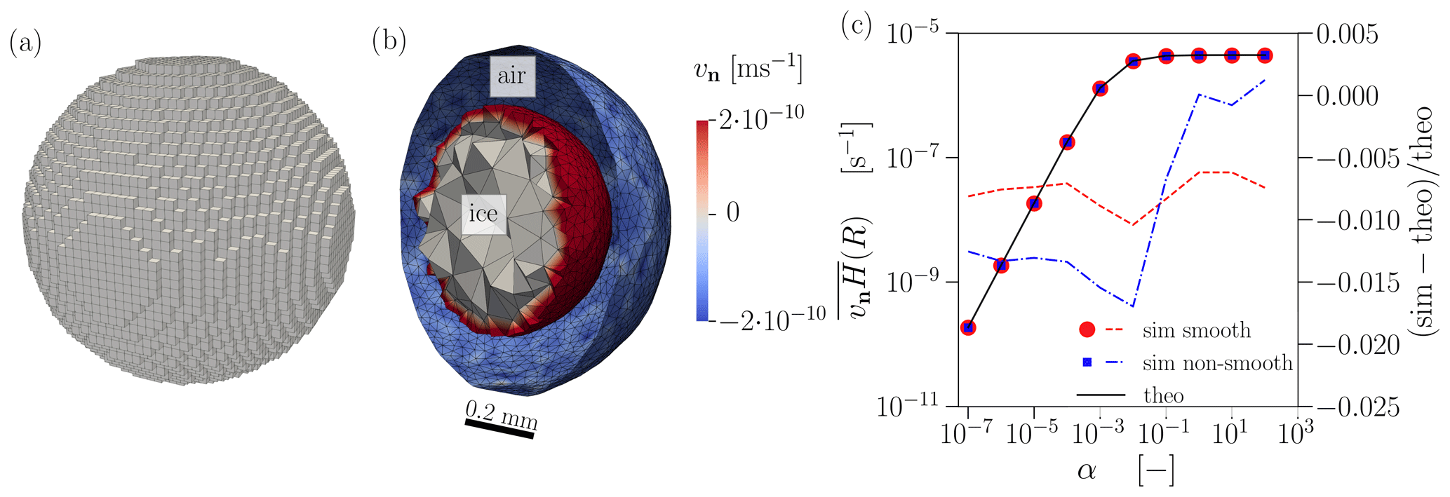
Figure 2(a) Voxel sphere obtained from a binary image and used to constrain the problem. (b) Clip of the outer and inner spherical shells with visible elements colored according to the interface velocity vn (sublimation in blue, deposition in red). (c) Comparison of the growth rate on the inner radius R of the theoretical (theo) and simulated (sim) solution of the spherical shell test case for different values of the condensation coefficient α. Two different surface mesh qualities, with smoothing (smooth) and without smoothing (non-smooth), are employed. The red dots, blue squares, and solid black line correspond to on the left y axis, while the dashed red and blue lines correspond to the simulation error on the right y axis.
4.1 Overview
As an overview and for a visual inspection of the microstructures and the rates derived from the FE solution, we show in Fig. 3 the initial and the final microstructure of both experimental series, each colored according to the interface velocity vn (computed using Eq. 17). This reveals the morphological differences at the end of both experiments, where the longer experiment (series 2) has evolved into a more pronounced depth hoar state with enhanced formation of cup crystals (Pinzer et al., 2012). The simulations from Fig. 3 were carried out for the condensation coefficient for series 1 and for series 2, which coincides with the best root mean square error (RMSE) agreement in Fig. 4c that is described in detail in the following section. As suggested by the analytical solution (Fig. 2c) or the sensitivity of the vapor fluxes by Fourteau et al. (2021a), the simulated SSA rates are highly sensitive to the condensation coefficient α.
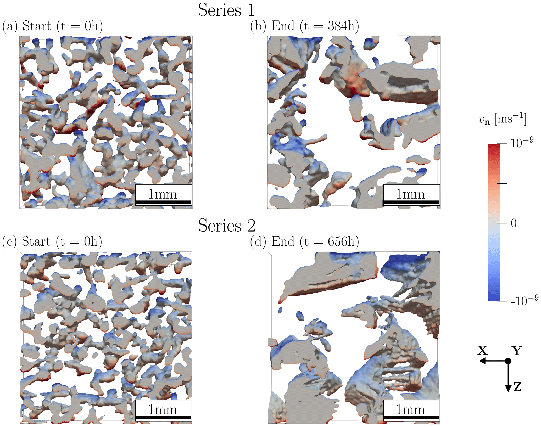
Figure 3Evolution of the ice–air interface, colored according to the interface velocity vn, demonstrated on cutouts of the length of 3.5 mm for (a, b) series 1 and (c, d) series 2.
4.2 Coarse temporal resolution modeling: α estimation
In the first step, we compare the temporal evolution of the SSA s in the experimental data and in the model using a large time step for the modeled data. For that, we downsample the experimental μCT time series to match the coarse temporal resolution and only perform FE simulations on those. Specifically, the modeled SSA values are computed with a coarse time resolution of Δ=48 h for series 1 (corresponding to 9 temporal points) and Δ≈60 h for series 2 (corresponding to 15 temporal points). This reduction in numerical effort allows us to perform a sensitivity study and estimate a value for the condensation coefficient α that best matches the experimental data. A fixed constant α is used for each simulation. The range of α varies from 10−3 to 1 for series 1 and from 10−3 to 10−1 for series 2. For the comparison with these simulated data, we simply use all available experimental SSA data (acquired for a temporal resolution of 8 h). The results are shown in Fig. 4a, b.
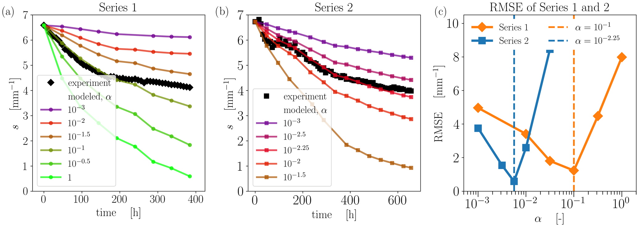
Figure 4Time evolution of the SSA s, experimental and modeled, with a varying condensation coefficient α for (a) series 1 and (b) series 2. (c) RMSE for both series.
We note that a few simulation points are missing in Fig. 4 due to the non-convergence of the FE solver. That being said, these missing points do not modify the overall decay of the simulated SSA time series. The best visual agreement between the experimental and the modeled data is found for for series 1 and for series 2. For series 1, the initial stage of the modeled curve with is close to the experimental data, while the final stage significantly underestimates the observed SSA. The same trend can be seen in series 2 although it is less prominent. The experimental data of series 2 reveal significantly more fluctuations in the initial phase, which is naturally not captured by the coarse-resolution modeling.
To assess the accuracy of modeled data quantitatively, the RMSE is computed according to
where N is the number of time steps involved in the modeling. The results are shown in Fig. 4c. The minimum of the RMSE curve coincides with the best visual agreement, i.e., and . The difference between the two optimal α values is 1 order of magnitude. Since the modeled curve for series 2 does not drop as much as the curve for series 1 in the final stage, the RMSE minimum for series 2 is lower despite higher data scattering.
4.3 Impact of temporal resolution
To assess the impact of temporal resolution on the modeled decrease in SSA, we performed simulations with the time step refined down to the time interval between two μCT images, namely 8 h. Based on results from the previous subsection, the simulations for the fine temporal resolution were carried out for the condensation coefficients and that were obtained by RMSE optimization of the coarse-resolution modeling. The results are given in Fig. 5. For series 1, the fine-resolution curve essentially coincides with the coarse-resolution one. The differences are slightly enhanced for series 2, where the fine-resolution curve lies slightly above the coarse-resolution one. The good agreement between the coarse-resolution and the fine-resolution simulations suggests that the coarse time step used in the previous section is sufficient to estimate the optimal α values.
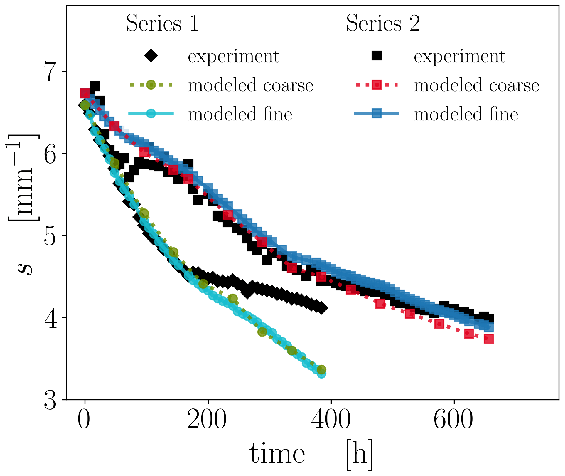
Figure 5The time evolution of the SSA s for both series with coarse and fine temporal resolution for the best previously found values and .
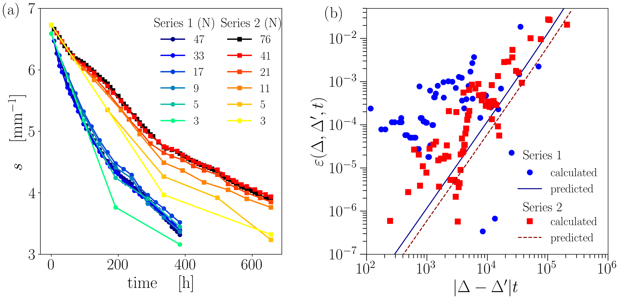
These modeled SSA differences due to different temporal resolutions can now be further assessed through the error metric from Eq. (25). To this end, we fix the values of α to the optimal values found in the previous section and compute the SSA evolution for various temporal resolutions. We choose different numbers of time steps N such that our model provides the time evolution of the SSA s(tn) with for different temporal resolutions, Δ and Δ′, where (cf. Fig. 6a). On the one hand, this allows us to calculate the error metric from Eq. (25) using the model results alone. The results are shown in Fig. 6b as solid markers for the two series. On the other hand, the error metric can also be independently estimated using the stochastic error model from Eq. (26) for the given variance σ. Fitting the variance using the least-squares method on the modeled data leads to values σfit=0.0007 and 0.0006 for series 1 and 2, respectively, and the results are shown in Fig. 6b as lines. These values are of the same order of magnitude as the variance computed as from the measurements, which is σmes=0.0005 and 0.0007 for series 1 and 2, respectively. Both estimations of the impact of the temporal resolution on the error metric are in reasonable agreement. Series 2 shows a significant difference in error between the coarsest and the finest temporal resolutions, both from simulations (red markers) and according to the μCT data (red line). On the contrary, the simulation-based estimation of series 1 (blue markers) does not drop as much for the finest temporal resolutions. This comes from the fact that the modeled SSA evolutions using our finest and second-finest temporal resolution substantially differ. Overall, the usage of the error metric indicates that the temporal resolution's impact on the SSA evolution remains relatively small, with errors below 1 %.
4.4 Signatures of a transition in α during TGM
Since we obtain a good agreement between experimental and modeled data for series 1 only in the initial stage, additional simulations were conducted to explore this further. As shown in previous research (see Fig. 6 in Krol and Löwe, 2018), series 1 undergoes a morphological transition at around t≈160 h, where up-facing and down-facing surfaces can be morphologically distinguished by their curvature distributions. From this time on, the second moment of up-facing and down-facing surfaces split up to follow a different dynamic. Such behavior during TGM is known from other work (Calonne et al., 2014a; Granger et al., 2021) and reflects the predominant emergence of facets on down-facing surfaces while the up-facing (sublimating) surfaces remain rounded. Here, we show that this morphological transition during TGM is consistent with a transition in the effective condensation coefficient α that governs the SSA decay. To reveal the different kinetic behavior of series 1 in the initial and final stages, we set the transition to – i.e., t=160 h – and performed independent optimization of the condensation coefficient. Very good agreement with the coefficient of determination R2=0.99 is achieved when the condensation coefficient is set to for the final stage. The results for the optimal parameters are shown in Fig. 7a.
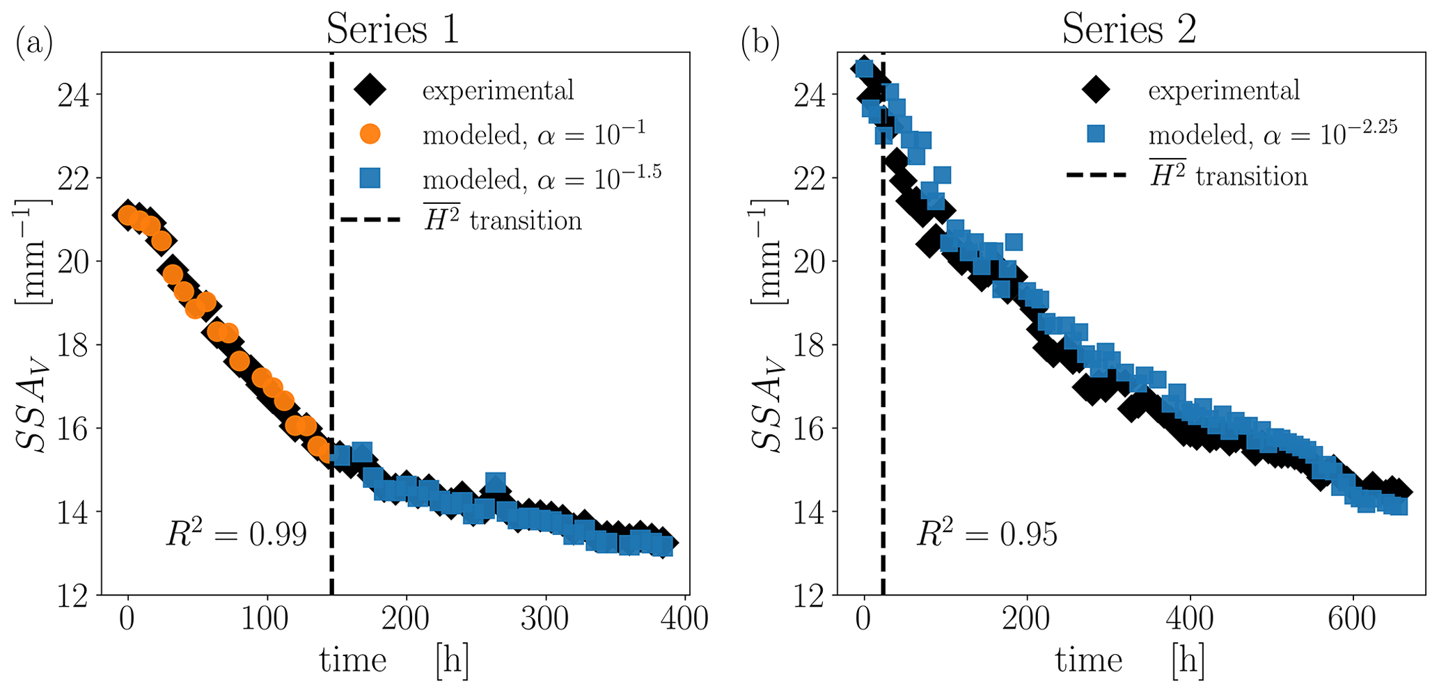
Figure 7Comparison of experimental and modeled SSA time evolution. (a) Series 1 with for t≤160 h and for t>160 h. (b) Series 2 with .
While the transition is also present in series 2 (Fig. 6 in Krol and Löwe, 2018), it occurs already very early in the time series after t≈24 h; see Fig. 7b. This is consistent with the observation that only one value of α is sufficient to match the measured data for series 2. Since the initial stage in series 2 is subject to higher fluctuations, an independent optimization of another α after a few time steps is inconclusive. Overall, this leads to the slightly reduced coefficient of determination, R2=0.95, for series 2. Figure 7 summarizes the best possible match we obtained for the SSA in the highest resolution within the developed method.
5.1 Modeling the SSA evolution from first principles
We set up a numerical model that can simulate the evolution of one of snow's most fundamental microstructural parameters, the SSA, from 3D μCT images. The model is based on the established theoretical description of snow metamorphism through coupled heat and mass diffusions at the pore scale (Kaempfer and Plapp, 2009; Calonne et al., 2014b). The solution of the diffusion problem thereby extends previous work characterizing TGM from μCT images (Flin and Brzoska, 2008; Pinzer et al., 2012; Krol and Löwe, 2016), where vapor fluxes were estimated only within the assumption of local equilibrium at the interface. Under this assumption, fluxes can be estimated from temperature fields and curvatures alone without explicitly solving the vapor equation. Our diffusion model is essentially physically equivalent to Kaempfer and Plapp (2009) in the steady-state limit and has been used previously (Fourteau et al., 2021a).
The actual novelty of our work is the combination of the numerical solution of the heat and mass diffusions with the exact surface area evolution equation (Krol and Löwe, 2018). This combination allows us to rigorously validate the SSA dynamics without explicitly evolving the ice–air interface in 3D space. This approach is thus complementary to 4D microstructure evolution models such as those inKaempfer and Plapp (2009) or Bouvet et al. (2022). The advantage of including the surface area equation (Eq. 9) in the analysis is the possibility of isolating the relevant growth rate for either constructing a stochastic error analysis (Sect. 3.4) or validating with analytical results (Sect. 3.5).
The model still requires considerable numerical resources, including the volume meshing of the microstructure, the FE solution of heat and mass diffusion equations taking into account kinetic effects of crystal growth, the extraction of the interface velocity vn from the vapor field, and the subsequent integration of the surface area equation. Nevertheless, we were able to reproduce the decay of the SSA during TGM for the first time from “first principles”, i.e., using a physical model and the actual microstructure without adjusting free parameters (in contrast to Legagneux et al., 2004; Domine et al., 2007; and Taillandier et al., 2007). The only unknown (physical) parameter in the model is the condensation coefficient, which characterizes vapor deposition and sublimation kinetics.
5.2 The condensation coefficient α
We have demonstrated that the SSA evolution in the model is highly sensitive to the condensation coefficient α (cf. Fig. 4). The best agreement (cf. Fig. 7) is obtained for values in the range (slightly different for the two time series) that fall in the intermediate range (Fourteau et al., 2021a) of possible values. This intermediate range of kinetics is compatible with neither the assumption of slow kinetics underlying the homogenization from Calonne et al. (2014b) nor the assumption of infinitely fast kinetics, which was previously used to compute vn from local temperature gradients (Krol and Löwe, 2016). While infinitely fast kinetics was already suggested to be inconsistent with the present experimental data sets (Krol and Löwe, 2018), this is now confirmed here from the estimated range for the values of α. From these results, we conclude that precise information about α is essential and that modeling the SSA during TGM solely using geometry and temperatures/gradients while neglecting kinetic effects (Flanner and Zender, 2006) cannot be justified.
It is well known that α is difficult to measure experimentally. This is explained in Libbrecht (2005) and can be easily understood from Fig. 2c. When α is commonly measured through the inversion of interface velocity vn data, the saturation form of the curve for the growth rate as a function of α implies significant uncertainties in α even for minor errors in the growth rate in the saturation region, where diffusion dominates. Our methodology can be considered to be a new (but similar) possibility of retrieving α by comparing simulated SSA evolution curves with experimental ones. From the reasoning given above, a high uncertainty should be expected. Surprisingly, the optimization (Fig. 4) reveals a rather sharp minimum. A similar procedure for obtaining α from the comparison of measured and modeled SSA curves was recently suggested by Bouvet et al. (2022), where a value of was obtained from a comparison of a phase field model with experimental data in isothermal metamorphism. The latter work put forward an interesting alternative route to the optimization of α from experimental data by means of dimensional analysis. So, instead of conducting many simulations of different values of α (as done here), the same results could be obtained through non-dimensionalization and a single simulation. However, the temperature gradient case considered here is governed by two different timescales instead of only one in the isothermal case (Bouvet et al., 2022), which renders this approach less straightforward in our case. When comparing our results to other data, we see that the obtained values of 10−1 and 10−1.5 for series 1 and of 10−2.25 for series 2 lie in the commonly found range of (Libbrecht and Rickerby, 2013), which is also used by Kaempfer and Plapp (2009). They are slightly higher than but of a similar order of magnitude to those reported in Fourteau et al. (2021a) and Bouvet et al. (2022). In contrast, the condensation coefficient from Jafari et al. (2020) translates to , which is significantly below this range.
In addition to the fact that both experimental series are apparently governed by a different condensation coefficient (Fig. 4), we provide evidence (Fig. 7) that the condensation coefficient may even change during a single experiment. To comprehend this finding, we recall that in snow, different parts of the ice–air interface belong to different crystallographic orientations and habits (rounded vs. faceted). Both have different attachment mechanisms and, therefore, different values of α (Libbrecht, 2005). Using a single, constant value of α that does not vary over the surface (as done here) must be therefore understood as an effective kinetic coefficient. This effective coefficient can capture actual microscale variations in α since a very good agreement for the SSA (as an integral property) is still obtained. It is quite remarkable that despite large variations in the condensation coefficient at the microscale, their collective behavior can be appropriately described through the use of a single α value. Indeed, in principle, the assumption of a constant α in Eq. (15) must be questioned on physical grounds. On facets, one expects that α is significantly reduced by orders of magnitude with a non-linear dependence on the ambient vapor field/supersaturation (Saito, 1996). Since facets cover only a fraction of the surface, this may explain why only a moderate drop in the effective α values (Fig. 7) is observed instead. Further substantiation of this hypothesis in future work is feasible even without crystal orientation measurements, which were, for instance, utilized in Granger et al. (2021). The surface area evolution equation (Eq. 9) and the pore-scale diffusion model can be easily extended to deal with spatially varying condensation coefficients on the ice–air interface and corresponding surface area sub-classes (e.g., up-facing and down-facing). Such a setup would allow us to validate the hypothesis for the condensation coefficient transition here. It would then be beneficial to include higher-order interfacial properties like and explicitly in the validation. This is, however, at the cost of evaluating higher-order rate terms.
5.3 Propagation of measurement errors
Our analysis has shown why high-quality μCT data are crucial for our methodology. The complex numerical workflow contains several sources of errors that may affect the predicted SSA evolution. First, experimental input data have a limited spatial and temporal resolution, which leads to missing structural and interface correlations between two consecutive images. However, with a different experimental setup, such as in Calonne et al. (2015), a higher spatial resolution may be achieved. Second, the volumes of interest considered here could be larger, in particular for series 2. This size might lead to some non-representativeness issues and small fluctuations in the measured SSA. This could explain the slightly noisy nature of the experimental parameter curves in series 2 compared to series 1. Third, all involved image analysis and simulation procedures come with additional numerical errors. While some uncertainties can be well controlled and assessed by testing the numerical workflow against analytical solutions (cf. Fig. 2), the existence of remaining errors is evident.
To address these errors and their impact on SSA modeling, we have exploited the fact that the explicit SSA representation allows us to construct a stochastic error model (Sect. 3). This model predicts how the combination of temporal resolution Δ, observation time t, and methodological errors (subsumed in the variance σ of the μCT comparison data) affects the SSA prediction. The stochastic model is reasonably consistent with the observed convergence of the predictions under reduction in the time step (Fig. 6). The fact that errors can be quantitatively addressed even without knowing the true SSA is facilitated by the representation of the SSA as a differential equation (Eq. 9). In the future, more sophisticated stochastic models should be envisaged and constructed from Eq. (9), which will further help to distinguish methodological noise and physics in the derived SSA dynamics.
5.4 Limitations and perspectives
Regarding model limitations other than the effective treatment of the condensation coefficient approach outlined above, we neglected the latent heat term in the interface condition for the temperature equation (Eq. 6). This leads to a slightly simpler numerical situation where heat and vapor are coupled in only one way, and the heat diffusion equation can be solved in advance. This strategy reduces the numerical cost of the method and facilitates the convergence of the iterative solver used in the FE software. Despite this simplification, we still observe that the vapor solver had issues to converge for a few microstructures, which explains a few missing points in the modeled time series (e.g., Fig. 5). The convergence of the FE simulations depends on the employed mesh and on the value of α. It could be facilitated by improving the mesh quality or increasing the maximum number of iterations. While this one-way coupling assumption eases the numeric, it was previously shown (Fourteau et al., 2021b) that for low-density or fast kinetics, latent heat significantly contributes to the heat fluxes in snow and may thus also impact the surface-averaged growth rate . This should be carefully investigated for low-density μCT time series under TGM in the future, where the numerical solution will become more demanding. In general, it would be advantageous to extend the analysis to other data sets. Here, we used only two TGM time series which have been well studied before (Kaempfer et al., 2005; Pinzer et al., 2012; Krol and Löwe, 2018). The evaluation of high-resolution TGM experiments with systematic variations in the control parameters (microstructure, temperature, and temperature gradients) would be desirable. This would allow us to parameterize the relevant growth rate from the control parameters, which is the most promising way to proceed towards a physically based SSA equation in snow cover models.
We have addressed the SSA evolution in TGM within a rigorous framework that combines the surface area equation with pore-scale heat and mass diffusion simulations. The comparison to experimental μCT data allowed us to estimate effective condensation coefficients that led to good agreement of the simulations with the measurements without further adjustable parameters. This shows that the evolution of SSA can be understood from the first principles of pore-scale physics (diffusive heat and mass transports), provided that the effective condensation coefficient α is well constrained. While this is a considerable step in understanding TGM, our results highlight the importance of independent estimates of the condensation coefficient in snow, which is indispensable to proceeding towards physically based SSA parameterizations in snow cover models.
We published simulation parameters and outputs for this study on the data portal EnviDat, https://doi.org/10.16904/envidat.492 (Braun et al., 2024).
AB and HL designed the study. AB and KF wrote the code. AB performed numerical computations. AB, KF, and HL discussed the data and wrote the paper. HL received the funding and supervised the study.
The contact author has declared that none of the authors has any competing interests.
Publisher’s note: Copernicus Publications remains neutral with regard to jurisdictional claims made in the text, published maps, institutional affiliations, or any other geographical representation in this paper. While Copernicus Publications makes every effort to include appropriate place names, the final responsibility lies with the authors.
Anna Braun and Henning Löwe would like to thank Michael Lehning for fruitful discussions. Kévin Fourteau's current position is funded by the European Research Council (ERC) under the European Union's Horizon 2020 research and innovation program (IVORI; grant no. 949516). We are thankful to Z. R. Courville and Thomas Kaempfer for reviewing the paper and to Masashi Niwano for editing it.
This research has been supported by the Swiss National Science Foundation (SNSF; grant no. 200020_178831).
This paper was edited by Masashi Niwano and reviewed by Z. R. Courville and Thomas Kaempfer.
Adams, E. and Brown, R.: A model for crystal development in dry snow, Geophys. Res. Lett., 9, 1287–1289, 1982. a
Albert, M. and McGilvary, W.: Thermal effects due to air flow and vapor transport in dry snow, J. Glaciol., 38, 273–281, 1992. a
Barrett, J. W., Garcke, H., and Nürnberg, R.: Numerical computations of faceted pattern formation in snow crystal growth, Phys. Rev. E, 86, 011604, https://doi.org/10.1103/PhysRevE.86.011604, 2012. a, b
Bouvet, L., Calonne, N., Flin, F., and Geindreau, C.: Snow Equi-Temperature Metamorphism Described by a Phase-Field Model Applicable on Micro-Tomographic Images: Prediction of Microstructural and Transport Properties, J. Adv. Model. Earth Sy., 14, e2022MS002998, https://doi.org/10.1029/2022MS002998, 2022. a, b, c, d, e, f
Braun, A., Fourteau, K., and Löwe, H.: Simulation parameters and outputs for a rigorous approach to the specific surface area evolution in snow during temperature gradient metamorphism, EnviDat [data set], https://doi.org/10.16904/envidat.492, 2024. a
Calonne, N., Flin, F., Morin, S., Lesaffre, B., du Roscoat, S. R., and Geindreau, C.: Numerical and experimental investigations of the effective thermal conductivity of snow, Geophys. Res. Lett., 38, L23501, https://doi.org/10.1029/2011GL049234, 2011. a
Calonne, N., Flin, F., Geindreau, C., Lesaffre, B., and Rolland du Roscoat, S.: Study of a temperature gradient metamorphism of snow from 3-D images: time evolution of microstructures, physical properties and their associated anisotropy, The Cryosphere, 8, 2255–2274, https://doi.org/10.5194/tc-8-2255-2014, 2014a. a, b, c
Calonne, N., Geindreau, C., and Flin, F.: Macroscopic modeling for heat and water vapor transfer in dry snow by homogenization, J. Phys. Chem. B, 118, 13393–13403, 2014b. a, b, c, d, e, f, g
Calonne, N., Flin, F., Lesaffre, B., Dufour, A., Roulle, J., Puglièse, P., Philip, A., Lahoucine, F., Geindreau, C., Panel, J.-M., Rolland du Roscoat S., and Charrier, P.: CellDyM: A room temperature operating cryogenic cell for the dynamic monitoring of snow metamorphism by time-lapse X-ray microtomography, Geophys. Res. Lett., 42, 3911–3918, 2015. a
Carslaw, H. S. and Jaeger, J. C.: Conduction of Heat in Solids, Oxford University Press, USA, ISBN 9780198533689, 1986. a
Colbeck, S.: Theory of metamorphism of dry snow, J. Geophys. Res.-Oceans, 88, 5475–5482, https://doi.org/10.1029/JC088iC09p05475, 1983. a, b
Coleou, C., Lesaffre, B., Brzoska, J.-B., Ludwig, W., and Boller, E.: Three-dimensional snow images by X-ray microtomography, Ann. Glaciol., 32, 75–81, 2001. a
Demange, G., Zapolsky, H., Patte, R., and Brunel, M.: A phase field model for snow crystal growth in three dimensions, npj Computational Materials, 3, 15, https://doi.org/10.1038/s41524-017-0015-1, 2017. a
Domine, F., Taillandier, A.-S., Houdier, S., Parrenin, F., Simpson, W. R., and Douglas, T. A.: Interactions between snow metamorphism and climate: Physical and chemical aspects, in: Physics and Chemistry of Ice, edited by: Kuhs, W. F., Royal Society of Chemistry, Cambridge, UK, 27–46, ISBN 978-0-85404-350-7, 2007. a
Domine, F., Taillandier, A.-S., and Simpson, W. R.: A parameterization of the specific surface area of seasonal snow for field use and for models of snowpack evolution, J. Geophys. Res.-Earth, 112, F02031, https://doi.org/10.1029/2006JF000512, 2007. a
Drew, D. A.: Evolution of geometric statistics, SIAM J. Appl. Math., 50, 649–666, 1990. a
Dumont, M., Brun, E., Picard, G., Michou, M., Libois, Q., Petit, J., Geyer, M., Morin, S., and Josse, B.: Contribution of light-absorbing impurities in snow to Greenland’s darkening since 2009, Nat. Geosci., 7, 509–512, 2014. a
Ebner, P. P., Schneebeli, M., and Steinfeld, A.: Metamorphism during temperature gradient with undersaturated advective airflow in a snow sample, The Cryosphere, 10, 791–797, https://doi.org/10.5194/tc-10-791-2016, 2016. a
Flanner, M. G. and Zender, C. S.: Linking snowpack microphysics and albedo evolution, J. Geophys. Res.-Atmos., 111, D12208, https://doi.org/10.1029/2005JD006834, 2006. a, b, c
Flin, F. and Brzoska, J.-B.: The temperature-gradient metamorphism of snow: vapour diffusion model and application to tomographic images, Ann. Glaciol., 49, 17–21, 2008. a, b
Flin, F., Brzoska, J.-B., Lesaffre, B., Coléou, C., and Pieritz, R. A.: Three-dimensional geometric measurements of snow microstructural evolution under isothermal conditions, Ann. Glaciol., 38, 39–44, 2004. a
Fourteau, K., Domine, F., and Hagenmuller, P.: Macroscopic water vapor diffusion is not enhanced in snow, The Cryosphere, 15, 389–406, https://doi.org/10.5194/tc-15-389-2021, 2021a. a, b, c, d, e, f, g, h, i, j, k, l, m
Fourteau, K., Domine, F., and Hagenmuller, P.: Impact of water vapor diffusion and latent heat on the effective thermal conductivity of snow, The Cryosphere, 15, 2739–2755, https://doi.org/10.5194/tc-15-2739-2021, 2021b. a, b, c, d
Granger, R., Flin, F., Ludwig, W., Hammad, I., and Geindreau, C.: Orientation selective grain sublimation–deposition in snow under temperature gradient metamorphism observed with diffraction contrast tomography, The Cryosphere, 15, 4381–4398, https://doi.org/10.5194/tc-15-4381-2021, 2021. a, b, c
Hagenmuller, P., Matzl, M., Chambon, G., and Schneebeli, M.: Sensitivity of snow density and specific surface area measured by microtomography to different image processing algorithms, The Cryosphere, 10, 1039–1054, https://doi.org/10.5194/tc-10-1039-2016, 2016. a
Hammonds, K., Lieb-Lappen, R., Baker, I., and Wang, X.: Investigating the thermophysical properties of the ice–snow interface under a controlled temperature gradient: Part I: Experiments & Observations, Cold Reg. Sci. Technol., 120, 157–167, 2015. a
Hanot, L. and Dominé, F.: Evolution of the Surface Area of a Snow Layer, Environ. Sci. Technol., 33, 4250–4255, https://doi.org/10.1021/es9811288, 1999. a
Harris Stuart, R., Faber, A.-K., Wahl, S., Hörhold, M., Kipfstuhl, S., Vasskog, K., Behrens, M., Zuhr, A. M., and Steen-Larsen, H. C.: Exploring the role of snow metamorphism on the isotopic composition of the surface snow at EastGRIP, The Cryosphere, 17, 1185–1204, https://doi.org/10.5194/tc-17-1185-2023, 2023. a
Hobbs, P. V.: Ice Physics, OUP Oxford, ISBN 9780199587711, 2010. a
Jafari, M., Gouttevin, I., Couttet, M., Wever, N., Michel, A., Sharma, V., Rossmann, L., Maass, N., Nicolaus, M., and Lehning, M.: The Impact of Diffusive Water Vapor Transport on Snow Profiles in Deep and Shallow Snow Covers and on Sea Ice, Frontiers in Earth Science, 8, 249, https://doi.org/10.3389/feart.2020.00249, 2020. a
Jafari, M., Sharma, V., and Lehning, M.: Convection of water vapour in snowpacks, J. Fluid Mech., 934, A38, https://doi.org/10.1017/jfm.2021.1146, 2022. a
Kaempfer, T. U. and Plapp, M.: Phase-field modeling of dry snow metamorphism, Phys. Rev. E, 79, 031502, https://doi.org/10.1103/PhysRevE.79.031502, 2009. a, b, c, d, e, f, g, h, i, j
Kaempfer, T. U., Schneebeli, M., and Sokratov, S. A.: A microstructural approach to model heat transfer in snow, Geophys. Res. Lett., 32, L21503, https://doi.org/10.1029/2005GL023873, 2005. a, b
Krol, Q. and Löwe, H.: Analysis of local ice crystal growth in snow, J. Glaciol., 62, 378–390, 2016. a, b, c, d, e, f, g, h, i
Krol, Q. and Löwe, H.: Upscaling ice crystal growth dynamics in snow: Rigorous modeling and comparison to 4D X-ray tomography data, Acta Mater., 151, 478–487, 2018. a, b, c, d, e, f, g, h, i, j, k, l
Legagneux, L., Taillandier, A.-S., and Domine, F.: Grain growth theories and the isothermal evolution of the specific surface area of snow, J. Appl. Phys., 95, 6175–6184, 2004. a, b, c
Li, Y. and Baker, I.: Metamorphism observation and model of snow from summit, Greenland under both positive and negative temperature gradients in a micro computed tomography, Hydrol. Process., 36, e14696, https://doi.org/10.1002/hyp.14696, 2022. a
Libbrecht, K. G.: The physics of snow crystals, Rep. Prog. Phys., 68, 855–895, https://doi.org/10.1088/0034-4885/68/4/R03, 2005. a, b, c, d, e, f, g, h, i, j, k, l, m
Libbrecht, K. G. and Rickerby, M. E.: Measurements of surface attachment kinetics for faceted ice crystal growth, J. Cryst. Growth, 377, 1–8, https://doi.org/10.1016/j.jcrysgro.2013.04.037, 2013. a, b
Malinen, M. and Råback, P.: Elmer finite element solver for multiphysics and multiscale problems, Multiscale Model. Methods Appl. Mater. Sci., 19, 101–113, 2013. a, b
Matzl, M. and Schneebeli, M.: Measuring specific surface area of snow by near-infrared photography, J. Glaciol., 52, 558–564, https://doi.org/10.3189/172756506781828412, 2006. a
Miller, D. and Adams, E.: A microstructural dry-snow metamorphism model for kinetic crystal growth, J. Glaciol., 55, 1003–1011, 2009. a, b
Picard, G., Löwe, H., and Mätzler, C.: Brief communication: A continuous formulation of microwave scattering from fresh snow to bubbly ice from first principles, The Cryosphere, 16, 3861–3866, https://doi.org/10.5194/tc-16-3861-2022, 2022. a
Pinzer, B. and Schneebeli, M.: Breeding snow: an instrumented sample holder for simultaneous tomographic and thermal studies, Meas. Sci. Technol., 20, 095705, https://doi.org/10.1088/0957-0233/20/9/095705, 2009a. a
Pinzer, B. R. and Schneebeli, M.: Snow metamorphism under alternating temperature gradients: Morphology and recrystallization in surface snow, Geophys. Res. Lett., 36, L23503, https://doi.org/10.1029/2009GL039618, 2009b. a
Pinzer, B. R., Schneebeli, M., and Kaempfer, T. U.: Vapor flux and recrystallization during dry snow metamorphism under a steady temperature gradient as observed by time-lapse micro-tomography, The Cryosphere, 6, 1141–1155, https://doi.org/10.5194/tc-6-1141-2012, 2012. a, b, c, d, e, f, g, h, i, j, k
Pokrifka, G. F., Moyle, A. M., Hanson, L. E., and Harrington, J. Y.: Estimating Surface Attachment Kinetic and Growth Transition Influences on Vapor-Grown Ice Crystals, J. Atmos. Sci., 77, 2393–2410, https://doi.org/10.1175/JAS-D-19-0303.1, 2020. a
Saad, Y.: Iterative Methods for Sparse Linear Systems, Society for Industrial and Applied Mathematics, ISBN 978-0-89871-534-7, 2003. a
Saito, Y.: Statistical physics of crystal growth, World Scientific, ISBN 978-981-02-2834-7, https://doi.org/10.1142/3261, 1996. a, b, c
Schleef, S. and Loewe, H.: X-ray microtomography analysis of isothermal densification of new snow under external mechanical stress, J. Glaciol., 59, 233–243, 2013. a
Schleef, S., Löwe, H., and Schneebeli, M.: Influence of stress, temperature and crystal morphology on isothermal densification and specific surface area decrease of new snow, The Cryosphere, 8, 1825–1838, https://doi.org/10.5194/tc-8-1825-2014, 2014. a
Schneebeli, M. and Sokratov, S. A.: Tomography of temperature gradient metamorphism of snow and associated changes in heat conductivity, Hydrol. Process., 18, 3655–3665, 2004. a, b
Schroeder, W., Martin, K., and Lorensen, B.: The Visualization Toolkit: An Object-oriented Approach to 3D Graphics, 4th edn., Kitware, New York, ISBN 978-1-930934-19-1, 2006. a
Schweizer, J., Bruce Jamieson, J., and Schneebeli, M.: Snow avalanche formation, Rev. Geophys., 41, 1016, https://doi.org/10.1029/2002RG000123, 2003. a
Shreve, R.: Migration of air bubbles, vapor figures, and brine pockers in ice under a temperature gradient, J. Geophys. Res., 72, 4093–4100, 1967. a
Taillandier, A.-S., Domine, F., Simpson, W. R., Sturm, M., and Douglas, T. A.: Rate of decrease of the specific surface area of dry snow: Isothermal and temperature gradient conditions, J. Geophys. Res.-Earth, 112, F03003, https://doi.org/10.1029/2006JF000514, 2007. a, b
The CGAL Project: CGAL User and Reference Manual, CGAL Editorial Board, 5.5.1 edn., https://doc.cgal.org/5.5.1/Manual/packages.html (last access: 5 June 2023), 2022. a
Van der Vorst, H. A.: Bi-CGSTAB: A fast and smoothly converging variant of Bi-CG for the solution of nonsymmetric linear systems, SIAM J. Sci. Stat. Comp., 13, 631–644, 1992. a
Wang, X. and Baker, I.: Observation of the microstructural evolution of snow under uniaxial compression using X-ray computed microtomography, J. Geophys. Res.-Atmos., 118, 12371–12382, https://doi.org/10.1002/2013JD020352, 2013. a
Wang, X. and Baker, I.: Evolution of the specific surface area of snow during high-temperature gradient metamorphism, J. Geophys. Res.-Atmos., 119, 13690–13703, https://doi.org/10.1002/2014JD022131, 2014. a
Wiese, M. and Schneebeli, M.: Snowbreeder 5: a Micro-CT device for measuring the snow-microstructure evolution under the simultaneous influence of a temperature gradient and compaction, J. Glaciol., 63, 355–360, 2017. a
Zermatten, E., Schneebeli, M., Arakawa, H., and Steinfeld, A.: Tomography-based determination of porosity, specific area and permeability of snow and comparison with measurements, Cold Reg. Sci. Technol., 97, 33–40, https://doi.org/10.1016/j.coldregions.2013.09.013, 2014. a