MMSeaIce: a collection of techniques for improving sea ice mapping with a multi-task model

The AutoICE challenge, organized by multiple national and international agencies, seeks to advance the development of near-real-time sea ice products with improved spatial resolution, broader spatial and temporal coverage, and enhanced consistency. In this paper, we present a detailed description of our solutions and experimental results for the challenge. We have implemented an automated sea ice mapping pipeline based on a multi-task U-Net architecture, capable of predicting sea ice concentration (SIC), stage of development (SOD), and floe size (FLOE). The AI4Arctic dataset, which includes synthetic aperture radar (SAR) imagery, ancillary data, and ice-chart-derived label maps, is utilized for model training and evaluation. Among the submissions from over 30 teams worldwide, our team achieved the highest combined score of 86.3 %, as well as the highest scores on SIC (92.0 %) and SOD (88.6 %). Notably, the result analysis and ablation studies demonstrate that instead of model architecture design, a collection of strategies/techniques we employed led to substantial enhancement in accuracy, efficiency, and robustness within the realm of deep-learning-based sea ice mapping. Those techniques include input SAR variable downscaling, input feature selection, spatial–temporal encoding, and the choice of loss functions. By highlighting the various techniques employed and their impacts, we aim to underscore the scientific advancements achieved in our methodology.

1 Introduction

Automated sea ice mapping using satellite data plays a vital role in understanding and monitoring the Earth's polar regions. Sea ice, a critical component of the cryosphere, undergoes significant spatial and temporal variations, impacting climate, ecosystems, and human activities. Satellite-based automated mapping techniques offer a unique advantage in providing comprehensive and frequent coverage over vast and remote areas. By employing advanced algorithms and machine learning (ML) approaches, these methods enable the efficient detection and characterization of different sea ice parameters (Lyu et al., 2022b). Accurate and timely sea ice mapping aids in climate modeling, facilitating climate change assessments, supporting operational activities such as navigation and resource management (Li et al., 2022), and enhancing our understanding of the intricate dynamics between the atmosphere, ocean, and ice-covered regions (Mahmud et al., 2022). The continuous advancements in automated sea ice mapping techniques using satellite data offer valuable insights into this fragile environment and aid in making informed decisions for sustainable development and environmental stewardship.

Deep learning (DL) has emerged as a powerful tool for sea ice parameter estimation from satellite data, especially dual-polarized synthetic aperture radar (SAR) imagery, revolutionizing the field with its wide-ranging applications and improved performance compared to traditional algorithms or conventional ML methods. DL-based models have demonstrated exceptional capabilities in accurately estimating crucial sea ice parameters such as sea ice concentration (SIC) (Wang et al., 2016, 2017; Cooke and Scott, 2019; Radhakrishnan et al., 2021; De Gelis et al., 2021; Stokholm et al., 2022; Malmgren-Hansen et al., 2020), stage of development (SOD) (Jiang et al., 2022; Lyu et al., 2022a; Chen et al., 2023a; Song et al., 2021; Khaleghian et al., 2021a; Liu et al., 2021a; Khaleghian et al., 2021b; Kruk et al., 2020; Boulze et al., 2020; Guo et al., 2023; Y. Zhang et al., 2021b; T. Zhang et al., 2021a; Kortum et al., 2022), and floe size (Chen et al., 2020; Nagi et al., 2021). These models leverage the ability of deep neural networks to automatically learn complex features and patterns from large volumes of data, enabling more robust and precise parameter estimation.

However, it is important to acknowledge potential areas for improvements of previous proposed DL-based methods. First, many existing models focus on estimating a specific parameter, which do not address the comprehensive characterization of sea ice in operational use. Second, a significant number of studies rely on data from a single sensor. Although this simplifies operational aspects and can enable the investigation of extracting its maximum value, it might lead to potential ambiguities and limitations in information integration. For example, although SAR images are capable of showing the spatial patterns formed by sea ice in high resolution, its backscatter intensities do not always distinguish between open sea in windy conditions and various ice surfaces (Malmgren-Hansen et al., 2020). In contrast, brightness temperature maps collected by radiometers such as the Advanced Microwave Scanning Radiometer 2 (AMSR2) satellite sensor can distinguish well between ice and open water but with coarse spatial resolution. Recent studies have implemented ML and DL-based methods for retrieving SIC from brightness temperature data and achieved promising results (Chi et al., 2019; Soleymani and Scott, 2021; Chen et al., 2023b). Third, due to the challenges in obtaining labeled samples for training, DL-based models for sea ice often suffer from limited volume of datasets, which can impact their generalization capabilities. Addressing these limitations is crucial to further enhance the effectiveness and applicability of DL-based sea ice parameter estimation methods.

Therefore, to address these challenges in automated sea ice mapping, the ESA (European Space Agency), DMI (Danish Meteorological Institute), the Technical University of Denmark (DTU), and NERSC (the Nansen Environmental and Remote Sensing Center) collaborated to create a sea ice challenge called AutoICE (Stokholm et al., 2023a, c). The goal of the challenge is to invite participants worldwide to derive more accurate and robust AI-based solutions of automated retrieval of multiple sea ice parameters, specifically, sea ice concentration (the percentage ratio of sea ice to open water, abbreviated as SIC), stage of development (the type of sea ice and its thickness, abbreviated as SOD), and floe size (the size and continuity of sea ice pieces, abbreviated as FLOE). A large volume of multi-source satellite and auxiliary data named AI4Arctic Sea Ice Challenge Dataset (Buus-Hinkler et al., 2022) are provided for the training and evaluation of the derived models.

In this paper, we present our methodology and corresponding outcomes that resulted in achieving first place in the challenge. Following the Introduction, Sect. 2 provides an overview of the AI4Arctic dataset used in this work. The methodology for the retrieval of sea ice parameters based on a multi-task U-Net, along with a collection of strategies employed for model performance improvement (e.g., SAR scene downscaling, input variable selection, spatial–temporal encoding, loss function selection), is illustrated extensively in Sect. 3. Experimental results with ablation studies are analyzed and discussed in Sect. 4. Finally, conclusions along with future research are summarized in Sect. 5.

2 Data overview

The Ai4Arctic dataset consists of 533 netCDF files, including 513 training files and 20 test files. Each training file contains dual-polarized Sentinel-1 Extra Wide (EW) swath images, AMSR2 passive microwave radiometer measurements, numerical weather prediction (NWP) parameters from ERA5 reanalysis dataset, and ice charts that follow the World Meteorological Organization (WMO) code for sea ice classes provided by either the Greenland Ice Service or the Canadian Ice Service. The 20 test files have the same parameters as the training files, except for the sea ice chart (label) data. There are two versions of the dataset available: a raw version and a ready-to-train version. The ready-to-train version undergoes additional processing steps to prepare it for deep-learning algorithms. To focus on model development and skip the initial preparation steps, we adopt the ready-to-train version to train our models. This version converts the original ice chart shapefile format into the netCDF format.

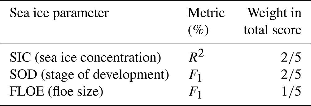
Each polygon in the ice chart is represented by an ID number and a table containing the ice chart variables for the polygon in the associated netCDF file. The SIC in each polygon represents the ratio of sea ice to open water in a given area, divided into 11 classes with 10 % increments, ranging from 0 % (open water) to 100 % (fully covered sea ice). In addition to total SIC, each polygon contains partial sea ice concentrations, associated with SOD and FLOE, which sum up to the total SIC. The partial concentrations are normalized by the total concentration to determine whether a partial concentration is dominant in each polygon. Dominant parameters are identified based on a threshold of 65 %. Therefore, a large portion of polygons do not have a dominant SOD or FLOE and are masked out from the labeling of SOD and FLOE. The SOD serves as an indicator of the sea ice type, which can be interpreted as a proxy for its thickness and ease of traversal. It consists of five classes: 0 represents open water, 1 is for new ice, 2 for young ice, 3 for thin first-year ice, 4 for thick first-year ice, and 5 for old ice (older than 1 year). The FLOE characterizes the size and continuity of sea ice floes, and it is defined by six classes: 0 for open water, 1 for cake ice, 2 for small floe, 3 for medium floe, 4 for big floe, 5 for vast floe, and 6 for bergs, which include various forms of icebergs and glacier ice. In addition, SAR scenes are downsampled to 80 m pixel spacing (around 5000 × 5000 pixels) for ease of use and to help reduce barrier to entry. The pixel values in the scenes are normalized within the $[-\mathrm{1},\mathrm{1}]$ range, and statistical information and class bins are provided. NaN values in SAR images are replaced with 2, and polygon ice charts are assigned a value of 255 to represent non-data or masked pixels. A detailed description of the dataset can be found in the manual provided by Buus-Hinkler et al. (2022). To evaluate the model performance numerically, SIC results are evaluated by calculating the R² coefficient, while SOD and FLOE maps are both evaluated using the F₁ score. The three sea ice parameter scores will be combined into one single final score as defined in the weighting scheme shown in Table 1.

Using ice charts as ground truths enables the classifier to extract the three sea ice parameters mentioned above at a regional level. Although pixel-based labels produced from the ice charts are provided in the ready-to-train version of the AI4Arctic dataset, they are generated based on a thresholding approach and cannot tell us about the locations of different ice types/floe sizes at SAR sensor resolution. That being said, the extraction of the sea ice parameters mentioned above at SAR sensor resolution is out of the scope of classification in this research. Besides, some other ice characteristics, such as thickness and drift, are also outside the scope of this research due to a lack of such information in the ice charts.

Table 1 The metrics for evaluating the three sea ice parameters and their weights in the final score specified by the competition.

3 Methodology

3.1 Network design and loss function selection

The network designed in this research is based on the architecture of a U-Net (Ronneberger et al., 2015) due to the following reasons. Characterized by the U-shaped structure, the network is able to capture both high-level contextual information and fine-grained details. Besides, the incorporation of skip connections facilitates the reuse of feature maps, addressing spatial information preservation and the vanishing gradient problem. Moreover, U-Net's demonstrated efficacy, particularly in scenarios with limited annotated data like sea ice mapping, underscores its ability to learn effectively from small datasets and generalize to new, challenging data environments. U-Net has shown success in many recent research studies concerning sea ice mapping (Radhakrishnan et al., 2021; Stokholm et al., 2022; Kucik and Stokholm, 2023; Nagi et al., 2021; Ren et al., 2021; Huang et al., 2021; Stokholm et al., 2023b). For example, in a recent study by Kucik and Stokholm (2023), a U-Net architecture was trained on the AI4Arctic Sea Ice Dataset version 2 (ASID-v2) (Saldo et al., 2021) to accurately retrieve SIC with different loss functions for performance comparison. Building upon this success, we extend the model to estimate three sea ice parameters concurrently. Our multi-task U-Net consists of four encoder–decoder blocks, with the first two blocks having 32 filters and the remaining blocks having 64 filters (as shown in Fig. 1). Alternative configurations, such as adding more blocks or increasing the number of filters, as well as employing state-of-the-art DL-based models for image segmentation such as the Swin transformer (Liu et al., 2021b), were explored. However, none of these approaches surpassed the performance of our current model.

To predict stage of development (SOD) and floe size (FLOE), we utilize the output feature maps from the final decoder and feed them into separate 1×1 convolution layers. Each convolution layer has a number of filters equal to the number of classes, enabling the generation of pixel-based classification results through segmentation. Regarding SIC estimation, as it can be treated as either a classification or a regression problem, we investigate both convolution and regression layers, employing different loss functions (e.g., mean squared error loss and cross-entropy loss) to compare their effectiveness.

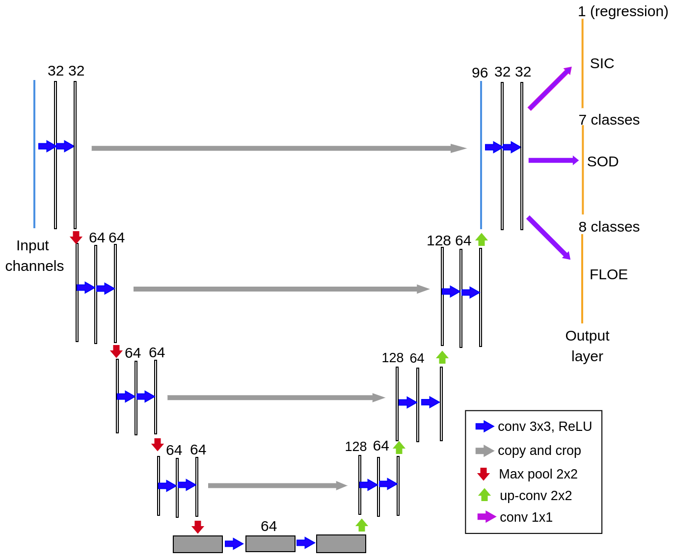
Figure 1 The structure of the proposed multi-task U-Net-based model with output layers in yellow.

3.2 Input SAR variable downscaling

Despite the resolution of the SAR imagery that is well suited for SAR sea ice monitoring, the polygon egg code data are derived from the knowledge of ice analysts who have to produce charts in low resolution due to time constraints. Therefore, to generate predictions consistent with the label maps, it is advantageous for input SAR image patches to encompass a large receptive field, which is achieved through the following operations. Initially, the dual-polarized SAR images, distance maps (DMs), and corresponding ice-chart-derived label maps are downsampled by a certain ratio (10 in the proposed model). During the training process, patches of size 256×256 are randomly extracted from the downsampled SAR images. As the AMSR2 and ERA5 inputs have been resampled to the Sentinel-1 geometry, their corresponding data points within the geographical areas covered by these patches are also interpolated to the size of 256×256. This downscaling operation has also been implemented in previous work (Liu et al., 2021a) concerning sea ice classification to avoid the appearance of scalloping and interscan banding artifacts in classification results.

After downscaling, data augmentation operations listed in Table 3 are applied to the extracted patches (with a probability of 0.5 for each operation) to enhance the model's generalization ability. During the validation and testing phases, the complete SAR scenes and DMs are downscaled, combined with other upsampled data inputs, and then fed into the trained model. The outputs are subsequently interpolated to match the original size of the SAR data and ice charts for evaluation purposes.

3.3 Ancillary data input selection

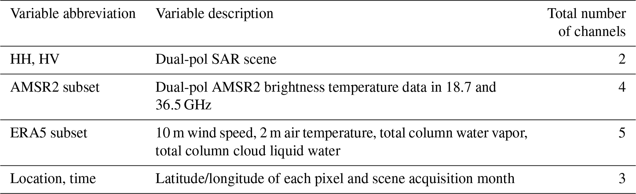
To select suitable inputs for training the model, we conduct experiments using various combinations of data inputs. Table 2 presents the combination of data inputs that yield the best performance. For the AMSR2 data, frequencies of 18.7 and 36.5 GHz are chosen due to their higher spatial resolution in comparison to lower-frequency channels, as well as their reduced sensitivity to atmospheric water vapor and cloud liquid water when compared to the 89 GHz channels (Minnett et al., 2019; Chen et al., 2023b). All ERA5 inputs in the AI4Arctic dataset are included, except for the skin temperature, which exhibits a high correlation with the 2 m air temperature and does not significantly improve overall accuracy. Detailed results using different combinations of input channels will be demonstrated and discussed in Sect. 4. The auxiliary data are brought up to input patch dimensions and added as channels in this research. Although it is also feasible to add them in the bottleneck, adding them as input channels facilitates us to analyze the effect of choosing different data inputs on model performance. Besides, it enables the convolutional neural network model to extract pixel-based nonlinear features at the very beginning. Nevertheless, in future works it would be interesting to compare the current channel adding approach vs. adding them in the bottleneck.

Table 2 The combination of data inputs that produces the highest combined score using the proposed model.

3.4 Spatial–temporal encoding

In operational sea ice mapping, ice experts not only rely on satellite data analysis but also utilize their domain knowledge, such as understanding typical ice conditions in specific regions during certain months in previous years. Additionally, SAR scenes captured in close proximity and similar time periods tend to exhibit comparable ice conditions. As the DL-based models proposed in this study lack access to such domain knowledge, we incorporate spatial and temporal information of each scene into the input channels, as illustrated in the last row of Table 2. Specifically, the latitude and longitude coordinates of the 21×21 Sentinel-1 SAR geographic grid points provided in the dataset are interpolated to match the size of the input SAR image. The time information of each pixel corresponds to the acquisition month (represented by enumeration, e.g., “01” for January) of the respective SAR scene. The incorporation of spatial and temporal information as data inputs originates from a previous work concerning the sea ice thickness estimation with Google Earth Engine and Sentinel-1 Ground Range Detected (GRD) data (Shamshiri et al., 2022). The reason to discretize time information instead of using continuous values (i.e., values specific to day) is that since the ice climatology is similar within 1 month, adopting continuous values might not improve model performance significantly. Besides, the imbalanced data distribution between different dates might lead to overfitting. In contrast, the data volume available for each month is relatively balanced. In future works, when the next version of the dataset is released (with around 16 times more data), it would be interesting to adopt the continuous approach for comparison. The effectiveness of spatial–temporal encoding in enhancing accuracy will be demonstrated in subsequent ablation studies.

3.5 Model training and implementation

The specifications of model training are detailed in Table 3, encompassing the combination of hyperparameters that yields the highest validation accuracy. Cosine annealing (Loshchilov and Hutter, 2016) is employed as our learning rate schedule, initially utilizing a large learning rate that gradually decreases following the cosine function to reach a minimum value, before rapidly increasing again (every 20 epochs in our model). This approach allows the model to navigate different regions of the loss landscape, potentially avoiding suboptimal local minima and converging to a favorable solution. To ensure sufficient exposure per data sample during training, each epoch comprises 500 iterations, with a batch of patches randomly extracted from training scenes during each iteration. Through exploring various combinations of loss functions, we observe that employing mean square error (MSE) loss for SIC and cross entropy (CE) loss for SOD and FLOE produces the highest testing accuracy. Specifically, the SIC retrieval is treated as a regression task, with a regression layer added before the SIC output in the model. Considering that the magnitude of MSE loss is considerably higher than that of CE loss, we assign a larger weight value (determined empirically) to the CE losses when calculating the total loss. This weight assignment facilitates the convergence of the three scores, as outlined in Table 3.

Table 3 Specifications of training the proposed model with the highest combined score, including hyperparameter values, learning algorithms, and loss functions.

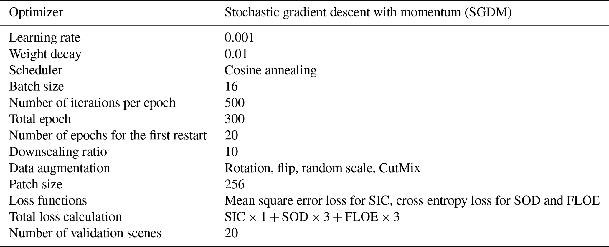
To validate the generalization capability of the model, for each experiment 20 SAR scenes from the training data are randomly selected as the validation set. Besides, to prevent the influence of randomness in parameters initialization and training, we train a total of 20 networks for each configuration and obtain the mean and variation of accuracy for more trustworthy performance evaluation. At the conclusion of each epoch, a combined score is calculated from the validation set, utilizing the metrics outlined in Table 1. If the score obtained in the current epoch surpasses all previous epoch scores, the model parameters are updated and saved. The final saved model is subsequently employed to generate predictions for the testing data submissions.

All experiments were conducted on the Narval cluster of Compute Canada, Canada's national high-performance computing system. The experiments utilized an NVIDIA A100-SXM4-40GB GPU with 128 GB of RAM memory, employing the PyTorch 1.12 library. It takes an average of about 3.5 h to train the proposed model.

4 Experimental results

Out of numerous submissions on the leaderboard, we achieved the highest combined score of approximately 86.3 %, as well as the highest SIC and SOD scores. As the ice-chart-derived labels for the testing data were released subsequent to the conclusion of the competition, we conducted additional model retraining using diverse configurations to obtain more comprehensive statistical outcomes for detailed analysis.

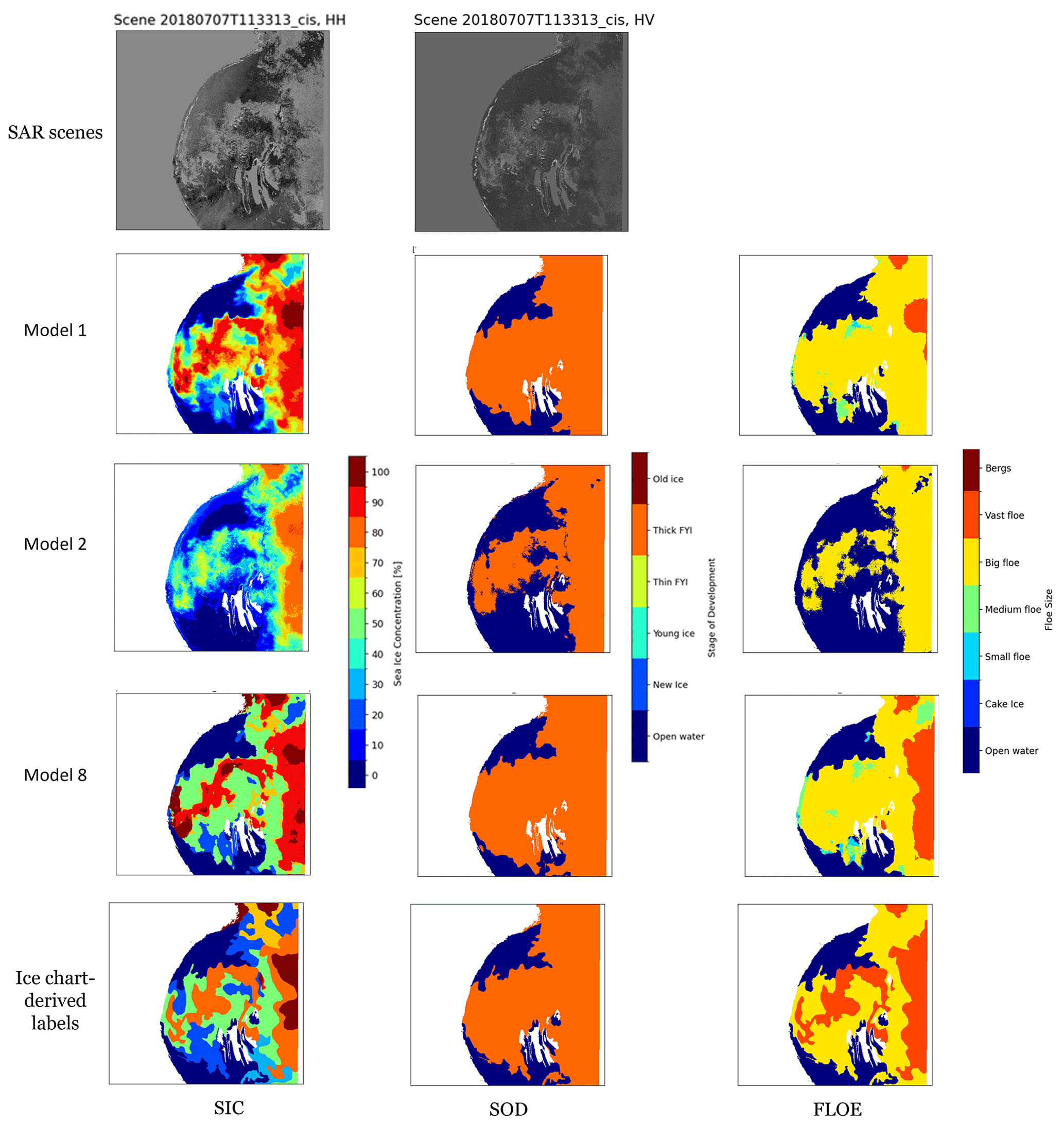
Figure 2 Sea ice mapping results obtained from a SAR scene (ID: 20180707T113313_cis) in the testing data using models trained with different configurations indicated by experiment numbers on the left. The ice-chart-derived labels are displayed in the last row for comparison. Areas that are land or without labels are masked in white.

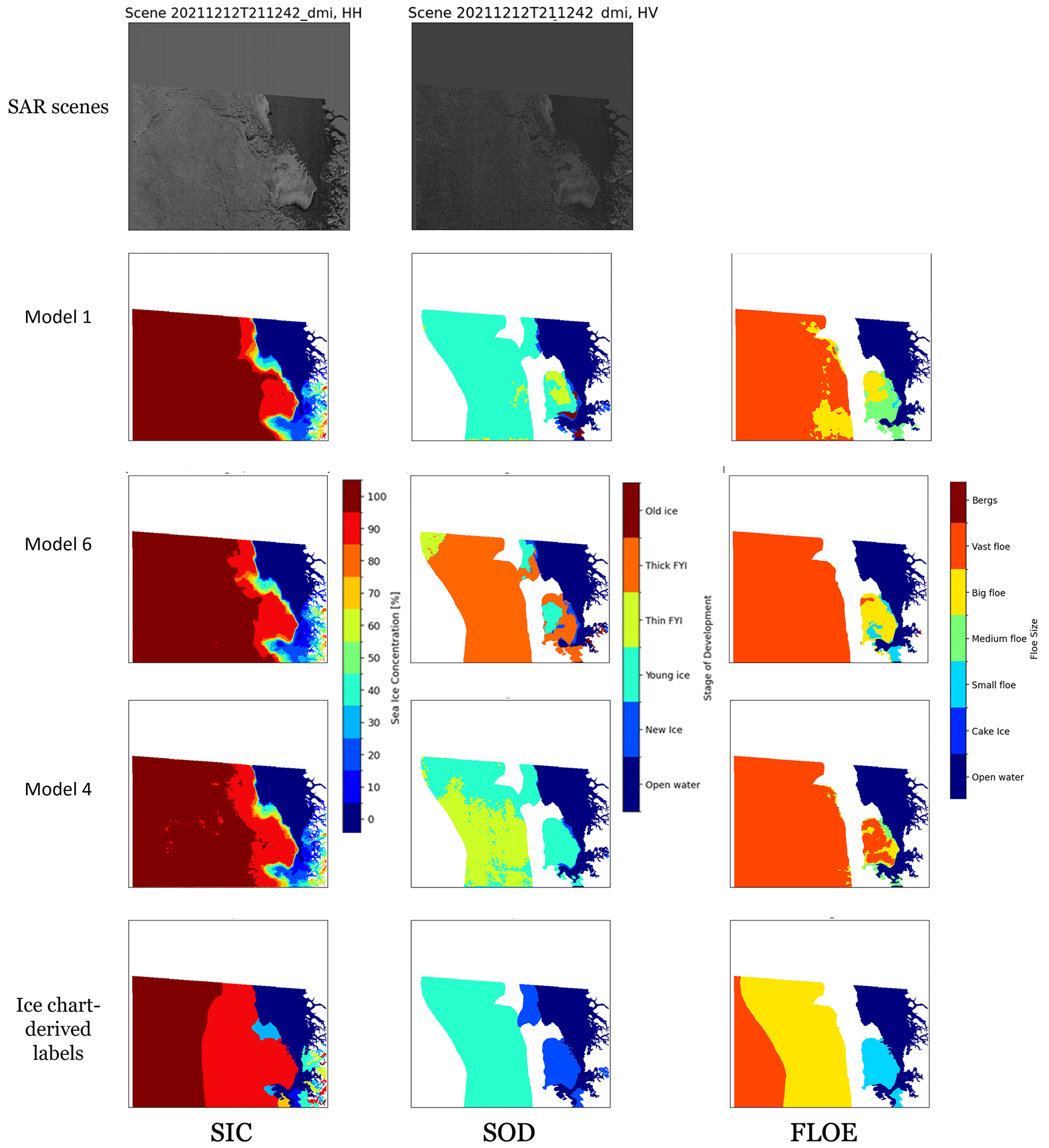
Figure 3 Sea ice mapping results obtained from a SAR scene (ID: 20211212T211242_dmi) in the testing data using models trained with different configurations indicated by experiment numbers on the left. The ice-chart-derived labels are displayed in the last row for comparison. Areas that are land or without labels are masked in white.

Table 4 The average default scores for SIC, SOD, and FLOE (i.e., R², F₁, F₁) obtained from models with different configurations. The average combined scores and the associated standard deviations are also calculated. Model 1 (full model) is developed using the specifications introduced in Tables 2 and 3. Compared to Model 1, Models 2–7 change the combinations of data inputs, Model 8 changes the loss function for SIC, and Model 9 splits the decoder into three separate parts for the three parameters. N/A means no modifications.

Figure 4 The confusion matrices of SOD (a) and FLOE (b) testing results.

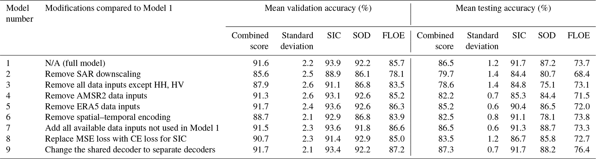
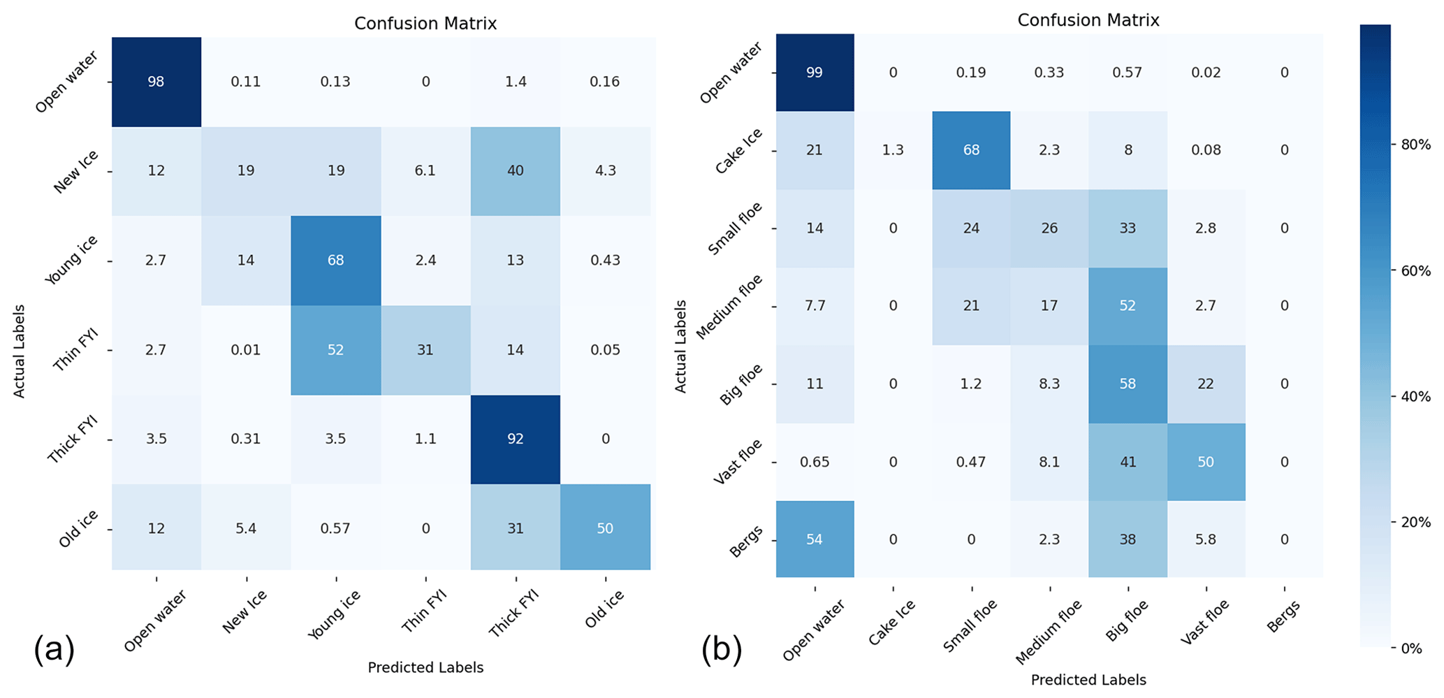
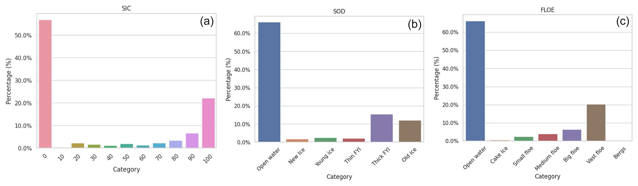
Figure 5 The distribution of training samples for each class in the three parameters (SIC on the a, SOD in the b, and FLOE on the c). The bars of some categories may be invisible due to very low percentages (e.g., 0.43 % for 10 % SIC, 0.48 % for cake ice, and 0.17 % for bergs in FLOE).

The statistical results obtained from model validation and testing are summarized in Table 4. Different configurations of trained models are represented by distinct model numbers (from Model 1 to Model 9), as specified in Table 4. Model 1 corresponds to the full model with settings described in Sect. 3 and Table 3. The remaining models serve as ablation studies to validate the effectiveness of the tricks we applied, with modifications detailed in Table 4. In the context of our study, conducting ablation studies on different data inputs enables a nuanced examination of their individual effects on the model's ability to accurately predict sea ice characteristics. This scientific approach aids in unraveling the intricate relationships between input features and model outcomes, guiding the optimization of model architectures and data preprocessing techniques for improved performance and interpretability. Each score in a certain model corresponds to the average score of the 20 networks trained with the same configuration. The relatively large standard deviation (SD) values of the combined scores in validation are caused by the randomness in validation scene selection. In contrast, the SDs of combined scores in testing are much smaller (around 1 %). Through comparison, the capability of those strategies in enhancing model performance is validated, as illustrated below.

• Model 1 (full model) vs. Model 2 (no downscaling). Downsampling the SAR data inputs significantly improves the mapping accuracy (Model 1 vs. Model 2), with improvements of 6.8 % in average testing combined score, 7.3 % in SIC, 6.5 % in SOD, and 5.3 % in FLOE. Furthermore, this downsampling enhancement also leads to a substantial increase in computational efficiency. Training the full model takes approximately 3.5 h while producing a map using the forward model for a SAR scene only requires an average of around 2 s. In contrast, without downsampling, the average training time is approximately 15 times longer. Various downsampling ratios were tested, and a value of 10 yielded one of the best results along with high efficiency.

• Model 1 (full model) vs. Models 3, 4, 5 (removing certain features). The inclusion of multi-source input channels is essential, as demonstrated by the comparison between Model 1 and Model 3. Using only SAR data inputs results in lower SIC and SOD scores by 6.9 % and 12.1 %, respectively. Although the removal of AMSR2 (Model 4) or ERA5 (Model 5) data inputs does not affect validation scores significantly, a drop in testing accuracy can be observed. This is particularly evident in the model without AMSR2 inputs, where the average SIC and SOD testing scores decrease by 6.4 % and 2.8 % compared to the full model. Thus, the inclusion of brightness temperature data plays a vital role in enhancing model accuracy.

• Model 1 (full model) vs. Models 6 (no spatial–temporal encoding). The effectiveness of spatial–temporal encoding in improving accuracy, particularly the SOD score, is evident in the comparison between Models 1 and 6. This is likely because the model in Model 1 can learn the distribution of dominant ice types in different Arctic regions during different months based on the training data, resulting in a 9.1 % improvement in average SOD score during testing. The inclusion of temporal and spatial information signifies the integration of sea ice climatology knowledge into the classification process. While this enhancement demonstrates improved model performance on recent data, it is essential to acknowledge the inherent limitations of relying solely on climatological information. The dynamic nature of the Arctic, undergoing continuous changes, emphasizes the continued reliance on observations from diverse sensors, such as SAR and passive microwave, ensuring that satellite data occupy a predominant role in the input channels for robust sea ice mapping.

• Model 1 (full model) vs. Models 7 (using all available data inputs). Compared to the model utilizing all available data as inputs (Model 7), the full model with feature selection (selecting a subset of AMSR2 and ERA5 data) achieves nearly the same accuracy while improving efficiency.

• Model 1 (MSE loss for SIC) vs. Models 8 (cross-entropy loss). Adopting MSE loss for SIC, as opposed to CE loss (Model 8), increases the average SIC testing score significantly by 5.0 % and improves the average testing combined score by 3.0 %.

• Model 1 (shared decoder) vs. Model 9 (separate decoders). Despite improvements in SIC and SOD scores, the FLOE scores remain relatively low, with a significant gap between validation and testing accuracy. After exploring numerous configurations, we found that only downscaling and separating the decoders for the three parameters (Model 9) might enhance the FLOE score. Visually, it is challenging to distinguish patterns of different floe sizes from SAR imagery. The mapping results of FLOE will be further discussed in the visual analysis below.

In addition to numerical results, visual interpretation is essential for analysis. Sea ice mapping results from two example SAR scenes in the testing data which were obtained using models with different configurations are presented in Figs. 2 and 3. Figure 2 illustrates that implementing input downscaling (including Model 1 and Model 8) enhances the consistency between the ice–water boundaries in the label maps and the model predictions. With a larger receptive field, contextual information is captured by the model, leading to spatially smoothed predictions. Conversely, without downscaling, the extracted features only contain local intensity information, limiting the model's ability to capture the presence of ice in surrounding areas, as demonstrated in the row corresponding to Model 2. Although models with larger patch sizes (e.g., 512, 768) have been tried out, we find that these models perform much worse than a patch size of 256. This could be due to a consequence of utilizing a model with an insufficient receptive field for the patch size, which could be an area for further improvements to the model in future works. Various input scales have also been implemented in a previous work (Stokholm et al., 2022) concerning sea ice concentration estimation. Furthermore, while choosing CE loss for SIC yields lower accuracy than MSE loss, the predictions consist of larger polygons that visually align more closely with the SIC label map, as seen in Model 8. This finding is consistent with the observations in Kucik and Stokholm (2023).

Furthermore, the effectiveness of spatial–temporal encoding in improving SOD prediction accuracy can be observed by comparing Model 1 and Model 6 in Fig. 3. In Model 6, where spatial–temporal encoding is not applied, a large area labeled young ice is misclassified as thick first-year ice (FYI). The model without AMSR2 inputs (Model 4) also misclassifies a relatively large area as thin FYI. Despite achieving relatively high SOD accuracy, there are some classes with significant misclassification rates. For instance, as shown in the confusion matrices in Fig. 4, the classification accuracies for new ice and thin FYI are only 19 % and 31 %, respectively. Misclassifications between ice types with neighboring thickness are also prevalent. For example, 31 % of old ice samples are misclassified as thick FYI. These issues may be attributed to various factors, such as the highly imbalanced distribution of samples among ice types. As depicted in Fig. 5, new ice and thin FYI have the most and second least samples in the training data (comprising only around 2 % of the total). Additionally, the labeling method of SOD and FLOE in the ready-to-train dataset might contribute to these challenges. Although most polygons in ice charts contain multiple ice types and floe sizes, they are labeled with only the dominant classes due to a lack of pixel-based labels, leading to inevitable labeling errors. During the competition, we attempted several strategies to address the issue of sample imbalance, such as implementing focal loss (Lin et al., 2017). However, none of these approaches have significantly improved the accuracy of the minority classes so far.

5 Conclusions

In this paper, we present our MMSeaIce pipeline, which consists of a multi-task U-Net for automated sea ice parameter retrieval from the ready-to-train version. In particular, we implemented several tricks to improve model accuracy and efficiency. The techniques behind those tricks include input downscaling, feature selection, incorporating spatial and temporal information, and loss function design. First, to enable our model to learn contextual information within a large receptive field, we initially apply a downscaling operation to the SAR data inputs. This enhances the consistency between model predictions and ice-chart-derived labels, resulting in a remarkable improvement of 6.8 % in the combined score and significant enhancement in computation speed. Then, we conducted ablation studies to investigate the impact of different data inputs on model performance. These studies demonstrate the necessity of including brightness temperature data, which leads to a 4.3 % improvement in the average combined score, as well as the importance of incorporating spatial–temporal information, which contributes to a 4.0 % improvement in the combined score. Additionally, we show that other modifications to the model, such as applying the MSE loss in SIC retrieval during training and employing separate decoders for the three parameters, also improve the overall performance. The best model we developed achieves an average combined score of 87.3 % on the testing dataset, with average individual scores of 91.7 %, 88.2 %, and 76.4 % for SIC, SOD, and FLOE, respectively.

Despite our success in the competition, there are still several areas that require further investigation to derive robust and accurate automated sea ice maps with high resolution. For instance, it is crucial to propose a new labeling method that adequately addresses polygons with mixed ice types or floe sizes. Furthermore, with the upcoming release of an updated AI4Arctic dataset containing a significantly larger volume of data, we recommend retraining our full model to improve the predictive accuracy of the minority classes. Additionally, considering the spatial and temporal variation of sea ice in SAR imagery, training models specific to certain regions or seasons, particularly the melting season, would be a preferable approach for enhancing performance.